educational data mining: collection and analysis of score matrices
TRANSCRIPT

UNIVERSITY OF CALIFORNIARIVERSIDE
Educational Data Mining: Collection and Analysis of Score Matrices for Outcomes-BasedAssessment
A Dissertation submitted in partial satisfactionof the requirements for the degree of
Doctor of Philosophy
in
Computer Science
by
Titus deLaFayette Winters
June 2006
Dissertation Committee:Dr. Thomas Payne, ChairpersonDr. Mart MolleDr. Christian Shelton

Copyright byTitus deLaFayette Winters
2006

The Dissertation of Titus deLaFayette Winters is approved:
Committee Chairperson
University of California, Riverside

Acknowledgements
I’m thankful to my advisor for aiming me sky high. I’m thankful to my wife for keeping
me grounded. I’m thankful to Eamonn for the inspiration and Christian for the direction.
I’m thankful to Sue, Todd, Mark, and Orit, for the opportunities they have given me. I’m
thankful to Phil for starting at the end of the alphabet. I’m thankful to Marian for putting
everything in perspective. I’m thankful for Steve for getting excited. I’m thankful to Vinh
and Eric for their help. I’m thankful for Dan for lunch. I’m thankful to Brian and Kris
for their support. I’m thankful to Peter for isolating the nastiest bug of the bunch. I am
particularly thankful for the support of my family and friends, for everything that has led
me to this point.
iv

ABSTRACT OF THE DISSERTATION
Educational Data Mining: Collection and Analysis of Score Matrices for Outcomes-BasedAssessment
by
Titus deLaFayette Winters
Doctor of Philosophy, Graduate Program in Computer ScienceUniversity of California, Riverside, June 2006
Dr. Thomas Payne, Chairperson
In this dissertation we provide an overview of the nascent state of Educational Data
Mining (EDM). EDM is poised to leverage an enormous amount of research from the data
mining community and apply that research to educational problems in learning, cognition,
and assessment. Similar problems have been researched in the educational community
for over a century, but the enormous computing power and algorithmic maturity brought to
bear by data mining has proven to be more successful at many of these educational statistics
problems. The timing of these developments could not be better, given the current rising
importance of assessment throughout education, particularly in the United States. After
determining the structural commonalities between EDM projects, I detail my own EDM
assessment project, covering tools for collecting, strategies for storing and archiving, and
v

new techniques for analyzing matrices of student scores. I also detail issues of real-world
deployment and adoption of this assessment system. After examining the state of EDM,
both in the abstract and with my own implementation and deployment, I predict near-term
trends in EDM and assessment, and conclude with thoughts on the implications of this
work, both for pedagogy and for the data mining community as a whole.
vi

Contents
Table of Contents . . . . . . . . . . . . . . . . . . . . . . . . . . . . . . . . .vii
List of Tables . . . . . . . . . . . . . . . . . . . . . . . . . . . . . . . . . . . .xi
List of Figures . . . . . . . . . . . . . . . . . . . . . . . . . . . . . . . . . . .xii
1 Introduction: The Importance of Assessment 1
1.1 Educational Data Mining. . . . . . . . . . . . . . . . . . . . . . . . . . . 4
1.2 Program Assessment at UC Riverside. . . . . . . . . . . . . . . . . . . . 6
1.3 Dissertation Overview . . . . . . . . . . . . . . . . . . . . . . . . . . . . 9
2 History & Background 11
2.1 Education & Educational Statistics. . . . . . . . . . . . . . . . . . . . . . 11
2.1.1 Psychometrics. . . . . . . . . . . . . . . . . . . . . . . . . . . .12
2.1.2 Theories of Cognition. . . . . . . . . . . . . . . . . . . . . . . . 16
2.1.3 Q-Matrix . . . . . . . . . . . . . . . . . . . . . . . . . . . . . . .20
2.2 Machine Learning and Data Mining Techniques. . . . . . . . . . . . . . . 21
2.2.1 Clustering. . . . . . . . . . . . . . . . . . . . . . . . . . . . . . .21
2.2.2 Dimensionality Reduction. . . . . . . . . . . . . . . . . . . . . . 25
2.2.3 Association Rules and Apriori. . . . . . . . . . . . . . . . . . . . 27
vii

3 Educational Data Mining, Spring 2006 29
3.1 ICITS04 . . . . . . . . . . . . . . . . . . . . . . . . . . . . . . . . . . . .30
3.1.1 EDM in 2004. . . . . . . . . . . . . . . . . . . . . . . . . . . . .30
3.1.2 Collection. . . . . . . . . . . . . . . . . . . . . . . . . . . . . . .31
3.1.3 Analysis . . . . . . . . . . . . . . . . . . . . . . . . . . . . . . .32
3.1.4 ICITS Workshop Summary. . . . . . . . . . . . . . . . . . . . . . 33
3.2 AAAI05 . . . . . . . . . . . . . . . . . . . . . . . . . . . . . . . . . . . .34
3.2.1 EDM in 2005. . . . . . . . . . . . . . . . . . . . . . . . . . . . .35
3.2.2 Storage. . . . . . . . . . . . . . . . . . . . . . . . . . . . . . . .35
3.2.3 Analysis . . . . . . . . . . . . . . . . . . . . . . . . . . . . . . .36
3.2.4 AAAI Workshop Summary. . . . . . . . . . . . . . . . . . . . . . 40
4 Data Collection 41
4.1 Agar . . . . . . . . . . . . . . . . . . . . . . . . . . . . . . . . . . . . . .42
4.1.1 History of CAA. . . . . . . . . . . . . . . . . . . . . . . . . . . .43
4.1.2 Agar. . . . . . . . . . . . . . . . . . . . . . . . . . . . . . . . . .45
4.1.3 Usage Patterns. . . . . . . . . . . . . . . . . . . . . . . . . . . .55
4.1.4 Conclusions. . . . . . . . . . . . . . . . . . . . . . . . . . . . . .56
4.2 HOMR . . . . . . . . . . . . . . . . . . . . . . . . . . . . . . . . . . . .56
4.2.1 Requirements. . . . . . . . . . . . . . . . . . . . . . . . . . . . .57
4.2.2 Internal Design. . . . . . . . . . . . . . . . . . . . . . . . . . . .59
4.2.3 Usage. . . . . . . . . . . . . . . . . . . . . . . . . . . . . . . . .64
4.2.4 Testing & Evaluation. . . . . . . . . . . . . . . . . . . . . . . . . 67
4.2.5 Sample Application: MarkSense. . . . . . . . . . . . . . . . . . . 69
4.2.6 Conclusions. . . . . . . . . . . . . . . . . . . . . . . . . . . . . .71
viii

5 Data Archiving 72
5.0.7 Gradebook Format. . . . . . . . . . . . . . . . . . . . . . . . . . 74
5.0.8 GnumeriPy. . . . . . . . . . . . . . . . . . . . . . . . . . . . . .75
6 EDM Analysis Notation and Data 77
6.1 Notation. . . . . . . . . . . . . . . . . . . . . . . . . . . . . . . . . . . .77
6.2 Data Sets . . . . . . . . . . . . . . . . . . . . . . . . . . . . . . . . . . .79
6.2.1 Course Data. . . . . . . . . . . . . . . . . . . . . . . . . . . . . .79
6.2.2 Online Quiz Data. . . . . . . . . . . . . . . . . . . . . . . . . . . 80
7 Question Evaluation 83
7.1 Good Questions. . . . . . . . . . . . . . . . . . . . . . . . . . . . . . . .83
7.1.1 Calculatingα andβ . . . . . . . . . . . . . . . . . . . . . . . . . 84
7.1.2 Assumptions. . . . . . . . . . . . . . . . . . . . . . . . . . . . .86
7.2 Results. . . . . . . . . . . . . . . . . . . . . . . . . . . . . . . . . . . . .87
7.2.1 Cross-Semester Consistency. . . . . . . . . . . . . . . . . . . . . 90
7.3 Question Evaluation Conclusions. . . . . . . . . . . . . . . . . . . . . . . 91
8 Predicting Missing Scores 92
8.1 Prediction Techniques. . . . . . . . . . . . . . . . . . . . . . . . . . . . .93
8.1.1 Matrix Average (Avg) . . . . . . . . . . . . . . . . . . . . . . . . 93
8.1.2 Student Average (RowAvg). . . . . . . . . . . . . . . . . . . . . 94
8.1.3 Question Average (ColAvg). . . . . . . . . . . . . . . . . . . . . 94
8.1.4 Student & Question Average (RowColAvg). . . . . . . . . . . . . 94
8.1.5 Difficulty & Discrimination (DD) . . . . . . . . . . . . . . . . . . 94
8.1.6 Conditional Probability (CondProb). . . . . . . . . . . . . . . . . 95
ix

8.1.7 Noisy OR (N-OR) . . . . . . . . . . . . . . . . . . . . . . . . . . 96
8.1.8 AdaBoost. . . . . . . . . . . . . . . . . . . . . . . . . . . . . . .96
8.1.9 Nearest Neighbor (NN). . . . . . . . . . . . . . . . . . . . . . . . 97
8.1.10 Topic Information . . . . . . . . . . . . . . . . . . . . . . . . . . 97
8.2 Educational Use and Implications. . . . . . . . . . . . . . . . . . . . . .100
8.3 Score Prediction Conclusions. . . . . . . . . . . . . . . . . . . . . . . . .101
9 Topic Clustering 103
9.1 Evaluation Method. . . . . . . . . . . . . . . . . . . . . . . . . . . . . .104
9.2 Algorithms . . . . . . . . . . . . . . . . . . . . . . . . . . . . . . . . . .105
9.2.1 Clustering. . . . . . . . . . . . . . . . . . . . . . . . . . . . . . .105
9.2.2 Agglomerative Correlation Clustering. . . . . . . . . . . . . . . .106
9.2.3 Dimensionality Reduction. . . . . . . . . . . . . . . . . . . . . .107
9.2.4 Educational Statistics. . . . . . . . . . . . . . . . . . . . . . . . .108
9.3 Results. . . . . . . . . . . . . . . . . . . . . . . . . . . . . . . . . . . . .112
9.3.1 Varying The Number of Factors. . . . . . . . . . . . . . . . . . .113
9.3.2 Independence of Input Size. . . . . . . . . . . . . . . . . . . . . .115
9.3.3 Free-Response vs. Multiple-Choice. . . . . . . . . . . . . . . . .118
9.3.4 Q-Matrix Model Mismatch. . . . . . . . . . . . . . . . . . . . . .118
9.3.5 Removing Low-Discrimination Questions. . . . . . . . . . . . . .123
9.4 Topic Clustering Conclusions. . . . . . . . . . . . . . . . . . . . . . . . .126
10 Clustering with Partial Topic Information 129
10.1 Hints Provided . . . . . . . . . . . . . . . . . . . . . . . . . . . . . . . .130
10.2 Algorithms . . . . . . . . . . . . . . . . . . . . . . . . . . . . . . . . . .131
10.2.1 k-means. . . . . . . . . . . . . . . . . . . . . . . . . . . . . . . .131
x

10.2.2 Agglomerative Clustering. . . . . . . . . . . . . . . . . . . . . .131
10.2.3 NNMF . . . . . . . . . . . . . . . . . . . . . . . . . . . . . . . .132
10.2.4 Q-Matrix . . . . . . . . . . . . . . . . . . . . . . . . . . . . . . .132
10.3 Results. . . . . . . . . . . . . . . . . . . . . . . . . . . . . . . . . . . . .132
10.4 Partial Information Conclusions. . . . . . . . . . . . . . . . . . . . . . .133
11 Future of EDM 137
11.1 Future Work. . . . . . . . . . . . . . . . . . . . . . . . . . . . . . . . . .138
11.1.1 Other “Baseline” Topics. . . . . . . . . . . . . . . . . . . . . . .138
11.1.2 Distinct Sizes of Cognitively Related Information. . . . . . . . . .139
11.1.3 Voting Methods for Topic Clustering. . . . . . . . . . . . . . . . .139
11.1.4 Alternate UI Platforms for Agar. . . . . . . . . . . . . . . . . . .140
11.2 The Road Ahead. . . . . . . . . . . . . . . . . . . . . . . . . . . . . . .140
12 Conclusions 143
12.1 Collection. . . . . . . . . . . . . . . . . . . . . . . . . . . . . . . . . . .144
12.2 Analysis. . . . . . . . . . . . . . . . . . . . . . . . . . . . . . . . . . . .145
12.3 Assessment. . . . . . . . . . . . . . . . . . . . . . . . . . . . . . . . . .147
12.4 Impact. . . . . . . . . . . . . . . . . . . . . . . . . . . . . . . . . . . . .148
Bibliography . . . . . . . . . . . . . . . . . . . . . . . . . . . . . . . . . . . .152
xi

List of Tables
6.1 Course Datasets. . . . . . . . . . . . . . . . . . . . . . . . . . . . . . . .79
6.2 Quiz Datasets. . . . . . . . . . . . . . . . . . . . . . . . . . . . . . . . .80
7.1 Sample Difficulty and Discrimination Values for Good Questions.. . . . . 89
7.2 Sample Difficulty and Discrimination Values for Bad Questions. . . . . . 90
8.1 Score prediction. . . . . . . . . . . . . . . . . . . . . . . . . . . . . . . .98
8.2 Score prediction with topic information. . . . . . . . . . . . . . . . . . . 99
9.1 Average Precision on Course Datasets, 2–9 factors. . . . . . . . . . . . .114
9.2 Average Precision within given Recall Ranges on Course Datasets, 8 factors114
9.3 Correlation of reconstruction accuracy vs. precision on binary datasets. . . 123
9.4 Average Precision on Highα items 2–9 factors . . . . . . . . . . . . . . .124
9.5 Average Precision on Highα items, 8 factors . . . . . . . . . . . . . . . .125
10.1 Precision vs. information provided. . . . . . . . . . . . . . . . . . . . . .136
xii

List of Figures
2.1 Dendrogram depicting the similarities of clustering algorithms. . . . . . . 24
4.1 Submission Manager. . . . . . . . . . . . . . . . . . . . . . . . . . . . .47
4.2 Rubric Creation. . . . . . . . . . . . . . . . . . . . . . . . . . . . . . . .49
4.3 Basic Grading Interface. . . . . . . . . . . . . . . . . . . . . . . . . . . .50
4.4 Creating or Editing a Comment. . . . . . . . . . . . . . . . . . . . . . . . 52
4.5 Agar Annotation Interface. . . . . . . . . . . . . . . . . . . . . . . . . . 53
4.6 Sample MarkSense Form. . . . . . . . . . . . . . . . . . . . . . . . . . . 58
4.7 HOMRConf: Generating a configuration for MarkSense. . . . . . . . . . 65
4.8 HOMR’s Three Basic Shapes. . . . . . . . . . . . . . . . . . . . . . . . . 66
4.9 A messy bubble grid that is processed perfectly.. . . . . . . . . . . . . . . 68
6.1 Sample IRT Graph. . . . . . . . . . . . . . . . . . . . . . . . . . . . . .78
7.1 Question Evaluation Example. . . . . . . . . . . . . . . . . . . . . . . . 85
8.1 Nearest Neighbor Classification Example. . . . . . . . . . . . . . . . . . 97
9.1 Best five algorithms, 008 dataset, six factors. . . . . . . . . . . . . . . . .109
9.2 Best five algorithms, 010 dataset, six factors. . . . . . . . . . . . . . . . .109
9.3 Best five algorithms, 141 dataset, six factors. . . . . . . . . . . . . . . . .110
xiii
9.4 Best five algorithms, Academic dataset, four factors. . . . . . . . . . . . .110
9.5 Best five algorithms, Trivia dataset, four factors. . . . . . . . . . . . . . .111
9.6 Best five algorithms, Academic dataset, Math & French only, two factors. . 111
9.7 Varying number of factors, 153 dataset. . . . . . . . . . . . . . . . . . . .115
9.8 Varying number of factors, 164 dataset. . . . . . . . . . . . . . . . . . . .116
9.9 Varying number of factors, Math & French data. . . . . . . . . . . . . . .116
9.10 Varying population size on Academic dataset, ICA (Clustered), 4 factors. . 117
9.11 Varying population size on Academic dataset, Math & French only, 2 factors117
9.12 Best five algorithms, 164 dataset, free-response only. . . . . . . . . . . .119
9.13 Best five algorithms, 164 dataset, multiple-choice only. . . . . . . . . . .119
9.14 Q-Matrix Reconstruction vs. Precision, 010 Dataset. . . . . . . . . . . . .121
9.15 Q-Matrix Reconstruction vs. Precision, 010 Dataset. . . . . . . . . . . . .121
9.16 Q-Matrix Reconstruction vs. Precision, Math & French. . . . . . . . . . .122
9.17 Q-Matrix Reconstruction vs. Precision, Math & French. . . . . . . . . . .122
9.18 Discriminationα cutoff vs. precision, 010 dataset. . . . . . . . . . . . . .126
9.19 Discriminationα cutoff vs. precision, 153 dataset. . . . . . . . . . . . . .127
9.20 Discriminationα cutoff vs. Precision, All Course Datasets. . . . . . . . . 127
10.1 Best four algorithms, 008 dataset. . . . . . . . . . . . . . . . . . . . . . .134
10.2 Best four algorithms, 141 dataset. . . . . . . . . . . . . . . . . . . . . . .134
10.3 Best four algorithms, Trivia dataset. . . . . . . . . . . . . . . . . . . . . .135
10.4 Best four algorithms, Math & French dataset. . . . . . . . . . . . . . . . .135
xiv

Chapter 1
Introduction: The Importance of
Assessment
As we advance into the twenty-first century, educators face new and growing assessment
requirements. The pressure for expanded assessment is coming from many directions at
once. The highest levels of government are holding public schools to greater accountabil-
ity (107th Congress of the USA, 2001). Accreditation organizations like ABET (ABET,
2005) are instituting policies that require understanding, acceptance, and compliance by
all instructors with new “continuous improvement” processes (Accreditation Policy and
Procedure Manual, 2002). In addition to (or possibly instead of) the fulfillment of the rela-
tively straightforward bean-counting requirements, accredited programs must now demon-
strate that they have established a “culture of assessment.” That is, it is still important that
appropriate material is being taught, but it is vital that an accredited program be contin-
uously monitoring the effectiveness of its instruction and demonstrate a willingness and
capability to react when problems are detected. Accreditation organizations like ABET are
trying to pull education away from “folk pedagogy” stemming from a lack of meaningful
1

quantitative information about the educational process, akin to the shift from Aristotelean
to Newtonian mechanics.
Unlike the ISO 9000 (ISO 9000, 2006) standards that have altered manufacturing and
business processes over the last ten years, educational outputs are difficult to measure. For
over a century, psychologists, cognitive scientists, and statisticians have studied ways of
putting a quantitative value on a person’s knowledge, but this has never been done reli-
ably without formal assessment and laboriously developed instruments. This is one of the
contributing factors behind the current push for standardized testing: without standardized
tests developed by professionals and issued to thousands or millions of students simulta-
neously, how can educators and administrators meet the assessment requirements being so
suddenly thrust upon them? If education were merely a manufacturing process, we could
measure, weigh, stress test, or run diagnostics on the product at the end of the process and
determine if our goals were being met. Without standardized tests, what is the analogue of
quality control in the educational domain?
At the same time, administrators and parents look to formal assessment processes as
a way of holding instructors accountable for their instruction. Most would argue that if
educators take these new requirements as an opportunity to embrace new technologies and
formalize educational standards and practices, these developments have the potential to
deeply alter the American educational system. Supporters of accreditation argue that if
this opportunity is seized, it will have a deeply positive influence on the quality of edu-
cation at all levels, just as the focus on continuous improvement has boosted performance
at ISO 9000 companies (O’Connor, 2005). But even if this potential for improvement is
realized, the new focus on assessment requirements represents a significant shift in educa-
tional practice, as the tradition has long been that instructors are allowed great flexibility,
both in instructional methods and material presented. It is no surprise then, that formal
2
assessment requirements are often looked upon as a burden by many college-level instruc-
tors (LeBlanc, 2002): regardless of potential for improvement, these new practices are
altering longstanding academic tradition.
In order to balance between the opportunities presented by the drive for assessment and
the independence of individual teachers, it is critical to develop assessment methods that
are as unintrusive as possible while still providing detailed quantitative assessment. In a
society adopting new digital technology at an astonishing rate, it is unsurprising that we
look to computing for possible solutions for collecting, storing, and analyzing all the data
that can be gathered on student learning.
Recent technological advances have significantly increased our ability to do just that:
collect, store, and analyze data. In the late 90s, the field ofdata miningsplit off from
the general artificial intelligence community. Unlike so many buzzwords of that era, data
mining followed through on much of its promise. Data mining provides solutions for such
problems as anomaly discovery, similarity matching on increasingly complex datatypes,
and the extraction of patterns and unseen structures, all while operating on vast volumes
of data. In many cases, data mining is solving similar problems to those that have been
dealt with for many years: dimensionality reduction and discovery of underlying genera-
tive factors are problems that have history dating back to the nineteenth century. In this
respect, data mining is well described by the epithet, “Statistics on steroids” (King, 2005).
The field has seen impressive growth since its inception, both in terms of volume of top-
quality research and the types of problems (Keogh et al., 2002; Kolter and Maloof, 2004)
that are becoming tractable by knowledgeable practitioners. Development of data mining
libraries like Weka (Witten and Frank, 2005) allow those who are not active researchers in
the area to readily make use of this research, and as the field develops it is expected to ma-
ture into standardized interfaces much as databases did in the 1970s and 80s. Data mining
3

has already radically altered the way that financial companies operate, playing a key role
in detecting credit card fraud or abuse of online services such as PayPal. Mortgage com-
panies increasingly rely on data mining techniques to predict who is a worthy credit risk.
Electronic trading houses are making immense profits on the stock and currency markets
by applying data mining techniques to identify profit opportunities in real time, effectively
creating money from nothing. Given the ever-growing importance of assessment, and our
general reliance on technological solutions, it is clear that at least some of those setting out
to solve our assessment problems will turn to data mining.
1.1 Educational Data Mining
Poised to meet the growing need for pervasive assessment is the nascent field of Educational
Data Mining (EDM). EDM focuses on the collection, archiving, and analysis of data related
to student learning and assessment. EDM is a very new and very small academic field. The
first publications to mention educational data mining were published in the last two years,
and there are likely fewer than thirty people in the world that identify themselves as being
a part of it.
As with all new fields, EDM has grown out of existing disciplines and is spreading
to overlap with new ones. Many of the researchers who are shaping EDM hail from the
Intelligent Tutoring System (ITS) community, where ready access to large quantities of
educational data make EDM a logical direction to advance in. EDM research shares some
commonalities with the Artificial Intelligence in Education (AIED) community. The anal-
ysis performed in EDM research is often related to techniques in psychometrics and edu-
cational statistics. EDM is poised to revolutionize, or at the very least enhance and expand,
the statistical methods used in education by bringing to bear the results of decades of re-
4
search in data mining and machine learning. Finally, given the computational backgrounds
of most EDM researchers, it is not uncommon to find data pertaining to students learning
computer science. As such, it is not surprising to find some overlap between the EDM
and Computer Science Education (CSE) fields. This overlap may become stronger in the
next few years as CSE naturally progresses toward more quantitative research and EDM
broadens away from its original ITS focus.
EDM also borrows much from the machine learning and data mining communities.
In truth, the term “Educational Data Mining” is a slight misnomer in that “data mining”
is generally associated with enormous datasets and much of the research is focused on
developing fast and efficient algorithms for finding meaning in the data. Few EDM projects
have data in such quantities. Although there are certainly datasets with thousands or even
tens of thousands of records, it is just as common to work with datasets of tens or hundreds
of records. It is likely that EDM will more commonly face problems of too little data, rather
than the general data mining problem of too much data. General machine learning research,
especially unsupervised or semi-supervised learning, has a more direct influence on EDM.
It is, however, important to note that EDM does share some usability features with general
data mining. Most importantly, well-developed and generalizable EDM techniques should
have few parameters and require little or no user intervention.
The structure of most EDM projects can be broken down into three parts: collection,
archiving, and analysis. Collection refers to the tools and tutoring systems used to record
the relevant information, be it student scores, answers to online quizzes, or events from
an Intelligent Tutoring System (ITS). Archiving is the process of storing and browsing the
collected data. For score data, this is a relatively minor issue, but for the vast quantities
of data generated by some ITSs this can be a significant task. Analysis brings to bear the
tools of machine learning and data mining on the collected data in an attempt to gain deeper
5
understanding of student learning, discover the relationships among questions, and possibly
develop deeper quantitative understanding of cognitive processes in general. Depending on
the EDM project, these three tasks will shift in relative complexity and importance, but all
three must be addressed in any EDM project.
1.2 Program Assessment at UC Riverside
Here at the University of California Riverside the Computer Science and Engineering de-
partment has undertaken a significant EDM project for program assessment. The project
has two main goals related to EDM. First we wish to quantify the amount each student has
learned each of the topics covered in our curriculum. These topics are referred to as the
objectivesof the course, and are commonly things of the form, “Students will have knowl-
edge of linked-lists.” The objectives for each course are agreed upon by faculty members
that teach that course. The second goal of this project is to quantify the level to which
our curriculum as a whole is meeting ourprogram outcomes. The program outcomes are
a set of general abilities we hope our majors have by the time they complete the program.
Program outcomes are very general traits like, “An ability to apply knowledge of math and
science.”
Direct measurement of either the course objectives or program outcomes is impossi-
ble. In the absence of professionally developed and validated assessment material like the
SAT (SAT Reasoning Test, 2006) or an IQ test (Binet, 1905) there is no absolute scale for
measuring knowledge. When working with a specific domain, like computer science (CS),
it is necessary to find an assessment tool for that domain. CS is particularly troublesome
in this respect, due to the speed with which the field advances. The Computer Science
GRE can provide some numeric assessment, but not every student attempts that test, nor do
6
the GRE administrators communicate detailed scores to undergraduate CS departments for
assessment purposes.
Rather than utilize standardized testing methods, we have chosen to focus on the assess-
ment that already happens during each academic year. In each course in our curriculum,
students are assessed with a variety of methods ranging from homework assignments and
programming projects to in-class tests and quizzes. Each homework, quiz, and test is made
up of questions that are, of course, individually written and graded by domain experts. Usu-
ally the scores from each question are aggregated into an overall score, and the scores from
each instrument (assignment, test, or quiz) in a course are further aggregated into an overall
course grade. Our assessment method focuses on collecting and analyzing this score data
at its finest granularity, recording scores for each student on each question.
The collection of scores for each of them students on then questions assigned in a
course can be viewed as anm× n matrix, called ascore matrix. Each course offering
produces a score matrixS, which may have missing entries due to students dropping the
course, not completing an assignment, or missing a test or quiz. To simplify analysis, the
columns ofSare usually scaled to 0..1. Our analysis challenge is then to develop a method
of relating the data inS to the course objectives and program outcomes.
To relate the scores inS to the course objectives, we assume a linear relationship be-
tween questions (columns inS) and thet distinct course objectives. This implies ann× t
matrix R, where thei, jth entry ofR is the relevance (in the range 0..1) of questioni to
objective j. This matrixR is known as therelevance matrixfor the course.
Given S and R, it is possible to perform several types of course assessment. If we
average each of the columns ofSwe get a 1×n vectorS, the average score on each question.
The average scores for each course objective are given asSR. If we sum or average the
rows of R, we get a measure of thecoverageof each objective in the course: how many
7
questions were asked that related to that objective? Both the average score per objective
and the coverage can be useful in analyzing the effectiveness of a course offering.
A more personalized assessment technique possible with the information inSandR is
to determine for each student which topic they have the lowest average score in. This is
easily done by finding the minimum entry in each student’s row of them× t matrix SR. If
SandRare kept up-to-date while the course progresses, an assessment system built on this
method can easily offer customized study suggestions to every student at any time.
Performing program assessment is largely similar to the techniques used for course as-
sessment. We assume that the course objectives for each course have a linear relationship
with our program outcomes. Therefore each course has acourse matrix C, where thei, jth
element ofC represents the relation of course objectivei to program outcomej. By aver-
agingSRfor each course and multiplying byC, we are given an estimate of how well our
curricula is preparing our students for the outcomes we have set. As with any continuous
improvement process, regular monitoring of these values allows us to detect and correct for
gaps and shifts in our curriculum, using an entirely data-driven approach.
However, the system as described above is hardly acceptable to instructors. Rather
than recording only aggregate scores for each student on each assignment, we are asking
instructors to provide us the full score matrixS. Although every question must be graded
individually whether or not we requestS, the recording of scores is a tedious process at
best. Our courses commonly issue between 20 and 200 (n) questions to class sizes ranging
from around 10 to over 500 (m). Clearly, manual entry of the data inS is unacceptable. In
order for this project to be successful, we must provide methods to facilitate the collection
of Swhile imposing as few absolute restrictions on the faculty as possible.
AlthoughSrepresents by far the largest input to the system, for many coursesR is large
enough to be a significant task. Courses have on the order of 5 to 10 course objectives (t),
8

meaning thatRcan have on the order of 100 to 1000 entries. Automating the generation of
R to the extent possible provides a much more palatable system for faculty members already
burdened with countless teaching and research tasks that have more obvious importance.
The final matrix components in our assessment system are the course matricesC. Our
department has 11 program outcomes, and each course has around 5 to 10 course objectives.
Neither the course objectives nor the program outcomes are expected to change regularly,
meaning that course matrices are likely to remain relatively stable from year to year. As
such, there appears to be little benefit to any attempt at automating the creation ofC for
each course.
Conceptually, the program assessment techniques presented here are simple, requiring
no more than rudimentary linear algebra. This could be made more complex using non-
linear techniques, but since there is no intrinsic dimensionality or well-known scale for
program assessment there is no need for additional complexity. What complexity there is
in our EDM project stems entirely from the collection ofSand attempts to generateR. It is
these issues that are addressed in this research.
1.3 Dissertation Overview
This dissertation is an effort to serve as an introduction to Educational Data Mining, as
well as to advance the current state of the art with respect to collection and analysis of
score matrices. The program assessment project detailed above serves as a connective
framework for independent pieces of EDM research organized around this theme.
The general organization of this dissertation is as follows. Chapter2 provides rele-
vant background for EDM, focusing both on topics of education as well as the machine
learning techniques that are being used in the EDM community. Chapter3 surveys the cur-
9
rent research and common themes in EDM as of this writing. I will then discuss in detail
the work that I have done in this area, detailing the three major phases of a large EDM
project. In collection (Chapter4), this will necessitate a discussion of Agar, my Computer-
Aided Assessment system and a cornerstone of my Master’s Thesis (Winters, 2004), as well
as my Homebrew Optical Mark Recognition (HOMR) system. Agar represents a signifi-
cant foray into demand-driven software evolution and interface design. HOMR is built on
techniques from computer vision and supervised learning for classification, allowing opti-
cal mark recognition (OMR) forms to be developed via a word processor, printed on any
printer, and scanned by any scanner. Chapter5 discusses the archiving methods utilized in
our project. EDM analysis forms the bulk of the dissertation. in Chapters6 through10,
I present four contributions to EDM analysis of score matrices and the influence of topic
information on that analysis. Finally, I discuss some potential avenues for future work
(Chapter11), both for my own research and for EDM as a whole, and discuss the conclu-
sions that can be drawn from current EDM research with regard to both education and data
mining (Chapter12).
10

Chapter 2
History & Background
In order to more easily discuss the current state of educational data mining and my own
research, it is useful to first look at the history that has brought educational research, as
well as data mining and machine learning, to where they are today. As these two fields are
immense and such an overview could easily grow into a work of hundreds of pages, this
chapter will focus only on those theories and algorithms that are actively cited by recent
EDM publications. In this way it is possible to highlight the most important contributions
and provide a starting point for readers interested in finding a deeper historical perspective.
2.1 Education & Educational Statistics
The educational community draws on research from a number of different areas, ranging
from statistics to cognitive science. Within the EDM community, the most germane fields
are those of psychometrics and cognitive psychology.
11

2.1.1 Psychometrics
At its root, the quantitative branch of education that is most applicable to EDM ispsycho-
metrics. Psychometrics dates back at least as far as nineteenth century researchers such as
Sir Francis Galton, who were the first to focus on measuring latent quantities of knowledge
and ability in the human mind (Pearson, 1914). These are difficult values to quantify, as
there is no direct way to measure them and no implicit units or dimensionality to such a
measurement. Over the past century and more, the field of psychometrics has developed
ways of compensating for this, developing implicit scales and methods of comparison that
require no absolute measurement.
Within the broad area of psychometrics there are several major theories that have shaped
the field over the last century and have influenced current EDM research. The two most
influential on EDM are Classical Test Theory (CTT) and Item Response Theory (IRT).
Classical Test Theory
Classical Test Theory is the earlier of the two branches of psychometrics applicable to
EDM. CTT is a catch-all term for a collection of statistical techniques developed over the
past century. The base foundation of CTT comes from the work of Charles Spearman,
whose development of common factor analysis (CFA) in 1904 became the primary area of
research in psychometrics for half a century (Spearman, 1904).
Working around the turn of the twentieth century, Spearman was a psychologist and
mathematician seeking to support his theories on intelligence. He noted that in many cases
student scores on individual test questions were highly correlated, and proposed one of the
earliest theories of intelligence, known asg-theory, wherein raw intellect is viewed as a one-
dimensional traitg. This theory is still in use in some areas of psychology and education
12

today. Indeed, the most common intelligence test in America today is a univariate estimate
of g: the IQ test (Binet, 1905) provides scores as a single value encoding the ratio of mental
age to physical age.
However, Spearman was not completely satisfied with the single-dimensionalg-theory.
Some data simply did not match the proposed model. Turning to his extensive math back-
ground and the then-new techniques for calculating correlations between measured values,
Spearman developed common factor analysis, which is still used today to understand large
quantities of data by discovering the latent factors giving rise to that data. CFA assumes
that a linear model off factors can describe the underlying behavior of the system, in this
case the ability of students to answer items correctly:
Mi, j = µ j +f
∑k=1
Wi,kHk, j + ε (2.1)
whereMi, j is the score for studenti on item j, µ j is a hidden variable related to the difficulty
of the item,W is a matrix giving the ability of each student with respect to each factor,H
is a matrix relating each factor to each item, andε is the noise in score measurement.
CFA has remained popular since its inception, but has had its detractors since the be-
ginning. One of the most commonly noted problems with CFA is that the resulting factors
are a set of vectors spanning some (possibly proper) vector subspace of the input matrix.
The ability for CFA to match the data remains unchanged for any rotation of those vec-
tors within that subspace, and there is no mathematical indication of which rotation best
separates the factors into human-understandable results. Additionally, as pointed out by
psychologist Raymond Cattell in 1966, there is no built-in method for CFA to determine
how many factors to extract from the input matrix. Cattell proposed a visual method, known
as the scree test (Cattell, 1966) for identifying the “correct” number of factors to extract.
13

Whether or not the scree test is utilized to determine the proper number of factors, the crit-
icism of CFA remains. Within current psychometrics there are still only heuristic methods
for determining the number of factors; some heuristics are numeric and some are visual.
Algorithmically, CFA uses standard principal-component analysis (PCA) on the corre-
lation matrix of the data. Both CFA and PCA are the standard methods for performing this
sort of factoring within the psychometrics community. The primary difference between
CFA and PCA being post-processing rotation of the resulting vectors in CFA.
CFA was notable in that it was the first quantitative theory for psychometrics that in-
cluded the concept oftest error, the idea that a student’s score on a test is not an absolute
measurement of knowledge but rather a random draw from their knowledge state. This
concept has since spawned a host of statistical estimation methods in psychometrics. It is
these CFA and these related methods that are collectively known as classical test theory.
For EDM purposes, the important concepts arereliability, internal consistency, and valid-
ity. Reliability is a measure of how certain the scores produced by an instrument are. A
common method for discussing reliability is test-retest reliability: if a student is given a test
and her score is recorded, and then all knowledge of the test itself is wiped out (questions
are not remembered, nothing is learned by the student on the test), how likely is the same
student to get the same score when immediately retaking the test?
Reliability cannot be measured exactly, but a number of approximating techniques work
in practice, including issuing alternate forms of the test with slight question variations, or
the more commonsplit-half correlation. In split-half correlation, only one form of the
instrument is given to the entire population. The questions are randomly partitioned into
two sets, and the correlation between scores on each half is calculated.
Internal consistency measures the extent to which the questions on a given instrument
are measuring the same trait. Internal consistency is highly related to reliability. Split-half
14

correlation, which is primarily viewed as a reliability statistic, is a reduced form of Cron-
bach’s Alpha statistic is the common measure of internal consistency (Cronbach, 1951).
Cronbach’s Alpha is a mathematical technique to calculate the average split-half correla-
tion across all possible random splits. Having a high internal consistency indicates that
everything on an instrument is testing the same concepts, and that those questions have
relatively low error rates in measurement.
Validity is a more difficult concept, attempting to provide an estimate of how much
scores on the instrument actually measure what they are intended to measure. This often
relies on outside comparisons and validation, and is generally harder to quantify.
Among the recognized branches of psychometrics the newest, and in some ways more
powerful, branch of psychometrics is Item Response Theory (IRT), the framework behind
many computer-adaptive tests such as the new GRE (Baker, 2001; Wim J. Van der Linden,
2000). IRT requires larger student populations than are generally found in a single course,
and thus is not directly applicable in our assessment project. However, some of the con-
cepts from IRT are useful for developing a simple method for modeling item difficulty and
estimating missing score data, as discussed in Chapter7. IRT parameterizes a distribution
of the probability that a student with a given level of ability,θ , will answer a given item
correctly. Usually thesecharacteristic curvesare represented with a two-parameter logistic
function:
P(θ) = 1/(1+eα(θ−β )) (2.2)
Hereβ governs the difficulty of the item andα governs the discrimination of that item.
Discrimination is related to how likely it is that a student with ability less thanβ can an-
swer correctly and how likely a student with ability greater thanβ may answer incorrectly.
These parameters are generally calculated for a set of questions using techniques similar to
15

expectation-maximization (Dempster et al., 1977). This technique requires input sizes of
hundreds or thousands of students to function correctly.
IRT is powerful in that it provides a quantitative scale for question difficulty and student
ability. However, much like the rotational-symmetry of results from CFA, IRT has an issue
of scale. There is no absolute scale onto which abilities or difficulties are projected, and
thus, without some initial “known” values for student ability or question difficulty, any
scalar multiple or additive constant applied to the difficulties and abilities is equally valid
under IRT. This is less problematic than the rotational symmetries of CFA factors, but does
add complexity to the application of IRT. In practice this is handled by introducing certain
definitions and assumptions, like the known numeric value of a perfect score on the GRE.
Since IRT quantifies difficultyβ and abilityθ on an absolute scale, it applies regardless
of question difficulty. Asking advanced questions to novice students will result in low
average scores, but will ideally still trace out a rising portion of the characteristic curve.
Asking the same question of advanced students will plot out a higher portion of the curve,
but according to IRT the extracted parameters of the curve will be the same in both cases.
IRT literature insists this is true, although experimental evidence to support this claim is at
best difficult to find.
2.1.2 Theories of Cognition
For as long as there have been studies in psychology, there have been theories about how the
mind knows things. The formation and evaluation of these studies is the field of cognitive
science. Cognitive scientists study issues of attention, perception, memory, language, and,
to a lesser extent, learning.
Psychology itself was wholly the realm of philosophers until the late nineteenth century.
The study of the mind had been a philosophical discourse taken up by Plato, Aristotle, and
16

many other philosophers up through Rene Descartes and John Locke. Psychology as an
experimental science is thought to have first appeared in the 1870s, established by Wilhelm
Wundt at the University of Leipzig (Rieber and Robinson, 2001). Cognitive science was
intimately linked to experimental psychology as a whole until the middle of the twentieth
century. In the 1950s, cognitive psychology emerged in a rush as a further specialization.
Some of the earliest papers cited as part of the cognitive psychology revolution are also
results that are often discussed in academic culture (Miller, 1956).
The aspects of cognitive psychology that are most applicable for EDM are those that
overlap with learning and education. These are primarily theories of how the mind or-
ganizes and retrieves information. Many of these theories have grown hand-in-hand with
research in so-called “strong” artificial intelligence, which attempts to replicate human
intelligence in software. Some are even defined in terms of Lisp subroutines and data
structures. These are collectively known ascognitive architectures. The current EDM in-
teraction with theories of cognition is focused onsymbolicsystems and theories. These
ideas correspond most closely with the common approach to AI in the 1970s and 1980s,
when it was believed that with a sufficient rule-set and set of symbols it would be possible to
create a human-like intelligence based purely on the logical manipulation of discrete sym-
bols. Most modern research focuses on probabilistic reasoning, that allows for a Bayesian
“probability of truth” approach,1 or connectionism, which argues that human-level intelli-
gence cannot be coded directly but must stem from the emergent behavior of many smaller
interconnected systems.
The cognitive theory most cited by EDM researchers is ACT∗, developed at Carnegie
Mellon University by John Anderson (Anderson, 1983). In ACT∗, knowledge is repre-
1The canonical example being: after hearing the statement “Tweety is a bird,” it is safe to assume withhigh probability that Tweety can fly, but there must remain a chance that Tweety cannot, for Tweety may infact be a penguin.
17

sented in different forms: procedural for skills, declarative for facts and trivia, and a con-
cept similar to registers in computer processors for iconic memory, representing those bits
of information currently being held most closely in short-term memory. The ACT∗ frame-
work was developed in the Lisp programming language to validate the ACT∗ theory of skill
acquisition detailed in (Anderson, 1983) and summarized in (Anderson, 1982). ACT∗ is an
attempt to explain the theoretical differences between declarative factual knowledge (fact
lookup) and procedural skill knowledge (skills and abilities).
ACT∗ primarily functions as a framework for representing the knowledge and its struc-
ture, leaving to other cognitive theories the issue of learning. The current incarnation of
ACT∗, ACT-R, has been applied to matters as varied as studies of human-computer inter-
action (Anderson et al., 1997) and subitizing (Peterson and Simon, 2000), the ability for
humans to rapidly identify small quantities without resorting to counting.
The information on learning in the cognitive science literature, especially on the cog-
nitive architectures like ACT∗, provides a wealth of knowledge that is unknown by most
instructors, and even many of those in the CSE and EDM communities. Of particular in-
terest to the CS Education community are the first two sentences of (Anderson, 1982):
It requires at least 100 hours of learning and practice to acquire any signifi-
cant cognitive skill to a reasonable degree of proficiency. For instance, after
100 hours a student learning to program a computer has achieved only a very
modest facility in the skill.
Even without the quantitative applicability, these sorts of results on learning are critical in
the educational process, but remain sadly unknown in the broader educational community.
Soar is another common cognitive architecture (Laird et al., 1987). Soar (once SOAR)
is similar to the ACT family of architectures in that it has different methods for representing
18

different types of knowledge. Soar omits the short-term memory modeled by ACT-R but
claims to be superior in that the Soar project is the only major cognitive theory that does
not need to assume that humans are capable of learning, but instead shows that learning is
an emergent property of the architecture. Soar solves problems symbolically, like ACT, but
learns new rules using slightly different methods. In many ways the two projects are com-
parable, although ACT might be described as a cognitive theory that is also a Lisp program,
while Soar is an Standard Meta-Language (SML) program that also models cognition. The
distinctions are obviously quite subtle, and are grounded in the background training of the
developers and the users.
The “Power Law of Learning” or “Power Law of Practice” provides a quantitative rela-
tionship governing cognitive tasks:
t = Xαn (2.3)
In its most common form, this law states that the reaction time on a particular task falls off
exponentially with the number of trials taken, meaning that practice improves performance.
After many investigations, this has been found to be near universal across test subjects and
tasks. Further research into the matter has suggested that it is in fact a result of the (actual)
cognitive architectures responsible for human learning. There is evidence to suggest that
the error rate on tasks such as applying a skill, recognizing when to apply a skill, or (in a re-
stricted form) retrieval of a particular fact exhibit this same relationship. Practice improves
accuracy, and a simple mathematical model can be constructed to quantify this result. This
is related to the common phrase, “steep learning curve.” Given the strong quantitative
nature of this result, it is clear why this is an enticing approach for EDM researchers.
19

2.1.3 Q-Matrix
Q-Matrix theory is based on work done in the 1980s and 1990s, primarily by Menucha
Birenbaum of Tel Aviv University and Curtis Tatsuoka of George Washington Univer-
sity (Birenbaum et al., 1993). Q-Matrix is another method of capturing the underlying
factors and abilities that give rise to a matrix of student scores. In the most simple case,
Q-Matrix is applied to a binarym×n score matrix.
Q-Matrix operates on this matrix along with the assumed number of underlying abilities
or factors,t. Each question is assumed to have a binary relationship with each of thet
factors. Each student is similarly assumed to have a binary ability in those factors. Thus
Q-Matrix is decomposing the input matrix into a binarym× t matrix of student abilities in
each of those factors, as well as a binaryt×n matrix of question relevance. A student is
assumed to answer a question correctly if and only if the factors relevant to that question
are a subset of their own abilities.
Q-Matrix was originally formulated as a method for identifying a student’s “knowledge
state” in a restricted domain based on the scores from tests in that domain. Most of the
initial research by Birenbaum and Tatsuoka focused on mathematics education. However
recent work by Barnes has expanded Q-Matrix into new areas in fault-tolerant teaching,
tutoring systems, and EDM (Barnes, 2003).
Most or all Q-Matrix solvers utilize gradient descent on the reconstruction error of the
matrix in order to find the optimal model to fit the data. Given an initial random configura-
tion, the algorithm finds the single best entry to toggle in the student matrix or the question
matrix in order to best reproduce the input matrix. As a discrete optimization problem
with a search space growing asO(2t∗(m+n)), this is a computationally intensive solution.
A linear programming formulation may reduce the running time and increase the solution
quality, but it does not appear anyone has developed such a solution.
20
2.2 Machine Learning and Data Mining Techniques
Working from the above background in education and cognitive science, EDM focuses on
the application of modern AI methods to student data. The following is a brief overview of
the methods that EDM has used to date.
2.2.1 Clustering
Clustering focuses on organizing objects into groups that are similar in some way. The
nature of that similarity depends on the clustering algorithm that is used, which in turn
reflects the presumed underlying model. Clustering is an unsupervised learning application:
no training data is required to calibrate the algorithms to your problem. Raw, unlabeled data
is fed into the clustering algorithm and clusters are reported.
Clustering is intrinsically a complex topic: there is no absolute measure of correctness.
If a collection of people are given a scatterplot and asked to cluster the data points, there
is no certainty of agreement. Given a set of points with known labels, we can survey the
accuracy of a collection of clustering algorithms on that dataset, but the best algorithm on
one dataset may be the worst on another. There is not a single “clustering problem,” but
rather a unique clustering problem for every dataset, or at least every data source.
Further, as shown by Kleinberg in (Kleinberg, 2002), it is impossible to develop a clus-
tering algorithm that satisfies certain basic properties desirable in clustering. Kleinberg
proves that it is impossible to achievescale-invariance, richness, andconsistencyin the
same clustering algorithm. Here scale-invariance is simply a lack of implicit scale: data
points measured in inches should yield the same clusters as those same data points mea-
sured in meters. Richness is the requirement that all possible partitions of the data are
possible outputs for the clustering algorithm. Consistency is the requirement that moving
21
points in the same cluster closer together while moving clusters further apart should pro-
vide the same output when re-clustered. These restrictions map out the trade-offs necessary
in all clustering algorithms.
k-means
The k-means algorithm (MacQueen, 1967) is the simplest common clustering algorithm,
performing reasonably well on a variety of problem types. Ink-means, it is assumed that
there arek cluster centers, points which are not necessarily part of the input that define the
canonical example of a point in each of thek clusters. If the cluster centers were known,
clustering is simple: each point in the input data is assigned to the nearest center under
some metric. This metric is generally Euclidean distance, although for high-dimensional
data some other metric may be used.
In order to determine the location of the cluster centers from the data,k-means simply
iterates to stability: randomly pickk points from the input as cluster centers. Then assign
each point in the input to the nearest cluster, and calculate new cluster centers by finding
the mean of each cluster. This process continues until no points change assignment, or
until the centers are moving only a negligible amount each round. This is not necessarily a
globally optimal set of cluster centers, so random restarts are commonly used.
The k-means algorithm has a number of shortcomings. The most commonly cited
among them is the issue of determiningk, for which there must usually be some prior
knowledge of the data. By specifyingk, this algorithm drops therichnesscondition: par-
titions with any number of clusters other thank are not possible. Other problems include
dimensional scaling: the clusters produced if one dimension is unfairly scaled relative to
the other dimensions will not generally be the same as an unscaled clustering. For problems
where there is no pre-determined scale for each dimension, this amounts to an extra param-
22
eter for each dimension, reducing the general applicability and out-of-the-box usefulness
of the algorithm.
Spectral Clustering
Spectral clustering (Fischer and Poland, 2005) is often implemented using linear algebra
techniques, but can be explained as a relatively simple graph-partitioning problem. Given
input dataX1,X2, . . .Xn, form the complete, weighted, and fully-connected graph where
the edge between pointsi and j is given weight equal to thesimilarity of those points. A
spectral clustering intok clusters is done by finding the minimum weight cuts in the graph
that disconnect it intok cliques. Again, ask is known, therichnesscondition is not satisfied.
In practice this is often done by generating then×n similarity matrixS, whereSi, j is
the similarity ofXi to Xj under some similarity measure, often Euclidean distance. Thek
eigenvectors with largest associated eigenvalues are extracted from this matrix, and another
clustering technique, oftenk-means is applied to the resultingk×n matrix.
Hierarchical Clustering
To overcome the need for a parameter representing the number of clusters and allow for
the richnesscondition, some algorithms producehierarchical clusters. In such a scheme,
the output from the clustering algorithm is not an assignment of data points to clusters, but
rather adendrogramrepresenting the relative similarity of every input to every other input.
This encodes every number of clusters, ranging from each item individually clustered to all
items clustered together. By searching down the dendrogram to the level where the desired
number of clusters is the same as the number of subtrees in the graph, it is easy to discover
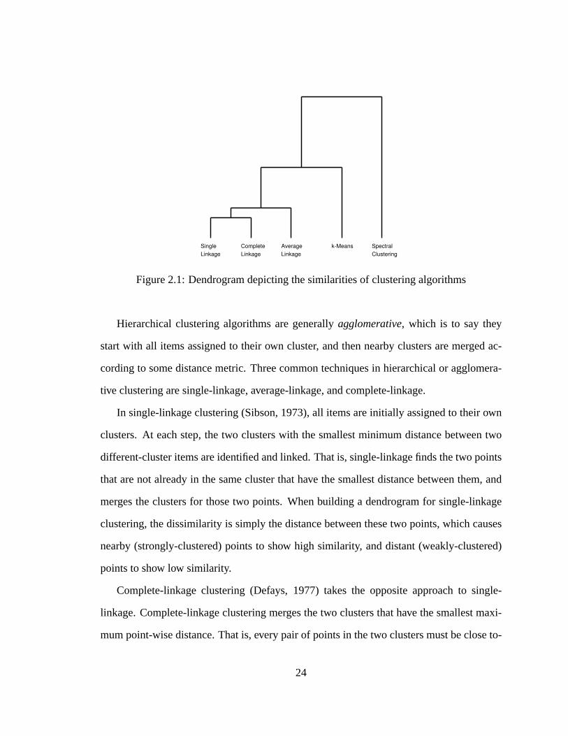
these clusters given the dendrogram. A sample dendrogram representing the similarity of
the clustering algorithms presented in this section is shown in Figure2.1.
23
SingleLinkage
CompleteLinkage
AverageLinkage
k-Means SpectralClustering
Figure 2.1: Dendrogram depicting the similarities of clustering algorithms
Hierarchical clustering algorithms are generallyagglomerative, which is to say they
start with all items assigned to their own cluster, and then nearby clusters are merged ac-
cording to some distance metric. Three common techniques in hierarchical or agglomera-
tive clustering are single-linkage, average-linkage, and complete-linkage.
In single-linkage clustering (Sibson, 1973), all items are initially assigned to their own
clusters. At each step, the two clusters with the smallest minimum distance between two
different-cluster items are identified and linked. That is, single-linkage finds the two points
that are not already in the same cluster that have the smallest distance between them, and
merges the clusters for those two points. When building a dendrogram for single-linkage
clustering, the dissimilarity is simply the distance between these two points, which causes
nearby (strongly-clustered) points to show high similarity, and distant (weakly-clustered)
points to show low similarity.
Complete-linkage clustering (Defays, 1977) takes the opposite approach to single-
linkage. Complete-linkage clustering merges the two clusters that have the smallest maxi-
mum point-wise distance. That is, every pair of points in the two clusters must be close to-
24
gether in order to be linked. This creates more tightly-grouped clusters than single-linkage,
which often creates clusters shaped like long chains of points.
Average-linkage (Sokal and Michener, 1958) uses the Euclidean mean of the clustered
points and finds the smallest distance between cluster centers.
The clustering property that is not held by these algorithms depends on the interpre-
tation of the dendrogram that is used to determine the clusters. If merging stops whenk
clusters remain, the algorithms again fail inrichness. If clustering stops when no clusters
are within some constant distance, these algorithms fail inscale invariance.If that distance
threshold is taken as a function of the maximum distance between two points in the input,
thenconsistencycan be violated.
2.2.2 Dimensionality Reduction
Another class of algorithms that have found use within current EDM research are numeric
algorithms for dimensionality reduction. These can be viewed in a number of ways, from
applicability to lossy compression, to explaining the variance in input data, to finding the
base factors generating the data. The algorithms presented here assume that the input ma-
trix X is based on a linear combination of those factors:X = UH.
Singular Value Decomposition
Singular value decomposition (Nash, 1990) is the method that best approximates the input
data in the reduced dimensionality, under the standard assumptions about least-squared
error. The resulting factors are an orthogonal basis that spans a subspace of the input
vector space. The factors are identified in order of importance by finding the direction of
highest variance of the input data until the desired number of factors has been extracted.
The elements ofU andH theoretically range−∞..∞.
25
SVD is generally considered to be the best tool to use for dimensionality reduction
when nothing is known about the underlying generative model of the data.
Independent Component Analysis
Independent Component Analysis (Hyvarinen, 1999a) is similar to SVD in that it identi-
fies a set of vectors that span a subspace of the input vector space. However, ICA is not
restricted to identifying orthogonal vectors. ICA is particularly suited to situations where
the data is a linear combination of non-orthogonal inputs.
This non-orthogonality has some important implication in the educational domain. If
the underlying factors are interpreted as “topics”, then an ICA factoring ofX into U and
H meansU is the student ability in each topic, andH is question relevance to each topic.
By not requiring topics to be orthogonal, topics can be discovered that have some overlap.
For example, we wouldn’t assume that ability with linked-lists is completely orthogonal to
ability with binary search trees. Both are recursive discrete structures, and they may share
some features in implementation. SVD would attempt to identify factors with no overlap
in this case, while conceptually ICA would better capture the relationship between topics.
Non-Negative Matrix Factorization
Another approach to dimensionality reduction is Non-Negative Matrix Factorization (Lee
and Seung, 2001). Rather than restricting the geometric properties of the resulting decom-
position, NNMF restricts the numeric properties. In NNMF, the entries ofU andH are
restricted to being non-negative. This has the effect of ensuring that each factor can only
contribute positively to the final results. This is particularly intuitive in the educational
domain, where questions do not have negative relevance to topic, and students do not have
negative ability in particular areas. Like Q-Matrix, NNMF is solved via gradient decent
26

with random restarts. However, as it is a continuous optimization problem, the optimum
direction to updateeveryentry inU andH can be computed at once, requiring far fewer
updates to reach a minima, and generally fewer restarts to reach a good fit.
2.2.3 Association Rules and Apriori
An area of data mining that has found great application in the business world is discovery
of association rules. Also known asMarket Basket Analysis, association rule discovery is
best understood through the ubiquitous supermarket example.
Imagine that every register receipt from a supermarket is stored in a central database.
The information stored in that database lists of all items purchased together (hence “market
basket”). Given a large database of these transaction logs, the question becomes, “Which
items are sold together?” Knowledge of the non-obvious item pairings that are most com-
monly seen appearing together in a transaction allows store owners to reorganize items on
the shelves to maximize the impulse buying behavior of their shoppers. The canonical ex-
ample is beer and diapers: in a hypothetical transaction database it is found that beer and
diapers have a tendency to be purchased together. It then makes marketing sense to capi-
talize on this by placing a beer display near the diapers in an attempt to increase impulse
buying of beer for those shoppers in the diaper aisle.
The Apriori algorithm (Agrawal et al., 1993) is the standard method for discovering
association rules from transaction databases. Apriori provides rules of the items that are
most commonly seen together, as well as a measure of thelift of items, the increase in
likelihood that itemY will be seen when the itemsX1 . . .Xn have been seen, when compared
to the overall odds of seeingY in the database.
Apriori has some relation to Q-Matrix in that both are discovering the most common
binary relationships in the data. However, Q-Matrix has an explicit generative model, while
27

Apriori is simply looking at the data and noting which features most commonly go together,
as well as which features “imply” which other features. Apriori is only identifying com-
mon patterns, not performing discrete optimization of the reconstruction error. As such,
although they have some similarity, Apriori is often significantly faster than Q-Matrix, and
may be suitable for use on some similar datasets.
28

Chapter 3
Educational Data Mining, Spring 2006
As of early 2006, Educational Data Mining is still such a young field that investigating and
describing its current state can be done by focusing on fewer than twenty papers published
in two workshops. Research that could be classified as EDM is also suitable in areas like
the International Journal of AI in Education (IJAIED) and the biennial Conference on AI
in Education (AIED). Most EDM research could also find some audience in the areas it
imperfectly overlaps with. In machine learning EDM is research can be viewed as a specific
and challenging application area. In education, EDM can function as a replacement for less
accurate but more established psychometric techniques. Currently, much EDM research
can also find an audience in the Intelligent Tutoring System (ITS) community, as a majority
of EDM researchers are focused on ITS data.
This chapter summarizes the state of EDM as of Spring 2006, focusing on the types of
research, general themes, and the leaders of the community.
29
3.1 ICITS04
The first of these formative workshops was held at the Seventh International Conference
on Intelligent Tutoring Systems in Maceio, Brazil. The workshop, entitled “Analyzing
Student-Tutor Interaction Logs to Improve Educational Outcomes”, was organized by Beck
of Carnegie Mellon University, and focused exclusively on the application of data mining
techniques to log data from ITSs.
3.1.1 EDM in 2004
At this workshop, Mostow presented an overview of EDM, although it is not yet called
such in his paper (Mostow, 2004). The paper details numerous ways in which additional
data-logging capabilities for ITSs can lead to improved knowledge of the system. Mostow
points out that such instrumentation and the type of collected data depends greatly on the
desired usage of the additional data.
Faculty may need simple summaries of student usage and progress; administra-
tors need evidence of ITS effectiveness; technical support staff need problem
alerts; content authors need usability indicators; developers need accurate bug
reports; researchers need detailed examples and informative analyses; and the
ITS needs parameters it can use, rules it can interpret, or knowledge it can be
modified to exploit.. . . Such informational goals are typically not clear at the
outset, instead emerging from and in turn guiding successively refined instru-
mentation and analyses.
Mostow goes on to enumerate a number of factors that make ITS data-minable, and
presents statistical values to be calculated or hypotheses to be investigated from canonical
30
ITS data. This enumeration presents a rough vision of many of the papers presented the
following year at the second EDM workshop.
3.1.2 Collection
Researchers from the HCI Institute at Carnegie Mellon and the Collide Research Group
of the University of Duisburg-Essen (Duisburg, Germany) presented an intriguing line of
research at the ICITS workshop (McLaren et al., 2004). Most ITSs are developed in what
is jokingly referred to as the “traditional” way, i.e., by putting together AI researchers and
programmers with domain experts for the ITS topic. The authors presented the idea of
taking logs from an environment in which students can experiment with the topic, and
from those logs building a skeletal ITS. The hope here is that in doing so they can predict
many of the errors that novices will make which domain experts are incapable of predicting,
reduce the time to creation, and provide additional insight for the experts when the system
is refined into a full-fledged ITS. This approach is referred to as “Bootstrapping Novice
Data” or BND.
A paper by Heiner, Beck, and Mostow points out the advantages to instrumentation of
ITSs to record data even with no anticipation of later analysis (Heiner et al., 2004). The
authors present multiple examples of data becoming useful only after it has been collected
with no anticipated use. The paper also discusses the difficulties inherent in collecting and
archiving the volume of data that can be recorded by a well-instrumented ITS, such as
Project LISTEN (Project LISTEN, 2006), the ITS project that much of the current EDM
community is involved with. The authors also address the general issues of data collection
and analysis that appear in most EDM projects. The paper goes on to discuss general diffi-
culties in working with large amounts of data, such as querying, processing, and presenting
the data in understandable ways.
31

3.1.3 Analysis
An EDM analysis paper by Koedinger and Mathan focuses on a variant of the Power Law
of Practice (Koedinger and Mathan, 2004):
E = Xαn (3.1)
whereE gives the error rate,X describes initial performance,n is integer valued and repre-
sents the number of opportunities to practice a skill that the student has had, andα gives the
learning rate for that skill. This formula comes from research done by Anderson, Conrad
and Corbett, showing that learning and mastery of atomic skills (skills that cannot be fur-
ther subdivided) is governed by this sort of power-law relationship (Anderson et al., 1989).
This assumes thatα is constant for all students attempting the given learning task.
Koedinger and Mathan explore the possibility thatα may take on a number of discrete
values representing qualitatively different modes of learning, focusing specifically on the
idea of the “intelligent novice” as a student with no prior experience but a general aptitude
for related topics. They present some initial findings, but do not go into great detail or
expand on the ideas presented. There appears to be quite a bit of work in this vein that could
be expanded on, and the authors’ CVs do not indicate that this work has been undertaken.
This might be considered a fertile field of future work for people entering EDM.
One final paper of note from the ICITS04 workshop came from researchers at Worcester
Polytechnic Institute (Freyberger et al., 2004). In this paper, Freyberger et al. present a
use for the Apriori association rule algorithm (Agrawal et al., 1993) to efficiently find
transfer rulesthat can be viewed as a generative model for student responses in ITS data.
These transfer rules govern the interaction between skills. For instance, given the skills:
“Calculate the area of a circle given its radius” and “Calculate the radius of a circle given
32

its area,” it is likely that practicing one of these may affect a student’s skill in the other.
Determining which of the atomic skills modelled by an ITS have such a skill transfer can be
a computationally expensive task. The researchers provide a method that finds an optimal
set of transfer rules, on their single dataset, with a factor of sixty speedup over a brute force
approach on that dataset.
3.1.4 ICITS Workshop Summary
Taking the papers presented at this workshop as a whole, a number of common themes and
connections to other areas emerge. Although the term “Educational Data Mining” doesn’t
appear anywhere in the proceedings, it is clear that there is a focus on issues of data mining
that transcend the ITS forum in which the workshop was held. Most of the papers focused
primarily on ITSs as a data source, but in many cases the algorithms being presented were
equally applicable to educational data acquired in another setting, such as a classroom test
or quiz. Authors like Freyberger, Koedinger, and Mathan apply modern machine learning
techniques to ITS data to make claims about educational issues of cognition and pedagogy.
Another clear theme in the ICITS04 papers is that of the multiple phases of EDM
projects. Both the Mostow and Heiner papers discuss issues of data gathering (and to a
lesser extent storage) for EDM tasks. McLaren’s bootstrapping technique (McLaren et al.,
2004) can be viewed as both gathering and analysis, by presenting a tool used to gather
the data that will be analyzed and synthesized into a new ITS. The majority of the research
presented is EDM analysis. Somewhere in the discussion that took place during the meet-
ing of these researchers it must have been noted that the research being discussed had a
stronger flavor of applied machine learning and data mining than much of the research at
ICITS, which has some machine learning but often focuses primarily on educational and
development issues surrounding ITSs. Within a few months of this workshop, a call for
33

papers for a second workshop was issued, now for the first time bearing the heading of
“Educational Data Mining.”
3.2 AAAI05
The workshop held in Pittsburgh as part of the American Association for Artificial Intelli-
gence (AAAI) conference in 2005 was also headed by Joe Beck, and attended by many of
the same people. Being a part of an AI conference rather than ICITS, much of the research
presented had a stronger flavor of machine learning than the work presented the previous
year. The separation from ICITS also gave the workshop the chance to attract people work-
ing on related projects that might not have a strong educational-technology background,
or might be focusing their efforts on data coming from non-ITS sources. According to
Beck, this was unanticipated: for many of the participants in the ICITS workshop, ITS data
was the material most suitable for analysis. ITS questions are already tagged with known
topics and are generally of high quality, the ITS is capable of providing skill estimates for
students, and the question text is available if needed. EDM on ITSs seemed so ideal that
the idea of people doing EDM on non-ITS data was “startling.” Yet, for the workshop,
which attracted ten accepted papers, there were data sources as disparate as standardized
tests (Hunt and Madhyastha, 2005), online quizzes (Barnes, 2005), and unmodified class-
room settings (Winters et al., 2005).
The papers presented at the workshop again present research at each level of EDM
design and development. None of the papers directly address data collection, but it is
referenced in (Mostow et al., 2005), (Barnes, 2005) and (Winters et al., 2005). Two papers
presented here refer to issues of common data formats and collaboration, focusing on both
collection and archiving. The majority of the papers, unsurprisingly, focus on analysis.
34

3.2.1 EDM in 2005
In a discussion of archiving, Mostow and a host of collaborators present an argument for the
importance of timestamps on ITS event data (Mostow et al., 2005). Within the surrounding
discussion of EDM is the following insightful summary of EDM research:
Educational data mining is an iterative cycle of hypothesis formation, testing,
and refinement that alternates between two complementary types of activities.
One type of activity involves aggregate quantitative analysis of many tutorial
events. For example, knowledge tracing analyzes growth curves by aggregat-
ing over successive opportunities to apply a skill. . .
In contrast, qualitative analysis focuses in depth on understanding individual
tutorial events. The research question it addresses is descriptive: “What hap-
pened when. . .?” Such case analysis can serve any of several purposes.
3.2.2 Storage
Aside from that summary, the research presented in (Mostow et al., 2005) focuses on a
browsing engine for tutorial events. If events are logged to an SQL database with certain
basic requirements on the log table (start time, end time, student, computer), the browser is
ITS independent. Other log fields are handled dynamically by the system. Written in Java
for portability, it allows fast SQL queries on the events in an attempt to help researchers
understand the information being produced by the ITS. It focuses strongly on the temporal
aspect of the data, providing varying granularity by building the virtual hierarchy of events
implied by the collection of start time/end time pairs on tutorial events being generated by
each ITS session. The tool was primarily built to work with Project LISTEN’s Reading
Tutorial (Project LISTEN, 2006), which in 2004 was listed as containing 54,000 sessions,
35
162,000 story readings, 1,634,000 sentences, 3,555,000 utterances, and 10,575,000 words.
Providing an interface to allow researchers to form hypotheses, examine average behaviors,
and investigate logged events is valuable regardless of data size, but critical when dealing
with such a volume of data.
3.2.3 Analysis
As expected, the majority of the papers presented in the AAAI workshop show a significant
machine learning background, with algorithms ranging from Expectation-Maximization (Jon-
sson et al., 2005) and gradient ascent algorithms (Barnes, 2005) to dimensionality reduc-
tion (Winters et al., 2005) and A∗ Search (Cen et al., 2005).
The most advanced AI leveraged for an EDM task in this workshop was presented
in (Jonsson et al., 2005). This paper is an investigation into learning the parameters for
Bayesian networks used to estimate student knowledge states in an ITS. It functions on
logs of ITS systems, inferring transition parameters for effectiveness of hints, initial skill
estimates, and learning rates. One feature the authors said was particularly important to
include was hidden nodes to encode skill mastery. As student skill mastery is truly a la-
tent trait, the addition of hidden nodes does make the model more intuitive than in other
Bayesian approaches to ITS modelling e.g. (Mayo and Mitrovic, 2001). The added com-
plexity of the resulting model is difficult to work with, especially with the goal of no hand-
coding of the various parameters. In order to learn the network parameters, the authors
use the Expectation-Maximization (EM) algorithm (Dempster et al., 1977) to match the
model to the input data. However, in order to validate that the correct parameters are being
learned, the input data had to be synthesized, and was synthesizedaccording to this model.
There is no strong evidence that such a model accurately captures the cognitive processes
of students interacting with an ITS. Given that the synthetic input data precisely matches
36

the model, it is unsurprising to learn that the Bayesian network parameters can be recovered
easily. Given the data source evaluated against, is it not particularly insightful to learn that
in such a system, problem difficulty does not have an effect on quality of model estimation.
There are a number of very interesting ideas presented in this work, but the experimental
design is unconvincing.
A paper by Hao Cen applies A∗ Search to a collection of expert-tagged features on var-
ious questions in an effort to match student performance on those questions to the accepted
ACT∗ learning model for an atomic skill (Cen et al., 2005). This model is detailed exten-
sively in (Nichols et al., 1995), and for skill-based questions (as opposed to fact-retrieval
questions) it is related to the aforementioned Power Law of Learning. The idea presented
is to use informed search to find the proper granularity of skills to be considered atomic in
the context of the given ITS, in much the same way that the Apriori algorithm was used to
discover skill-transfer rules in (Freyberger et al., 2004). The technique is evaluated on real
ITS log data, although with only a single dataset for the evaluation. Given the extensive
history and development of the ACT family of learning models (ACT-R, 2006), and the
results presented here, there seems to be much promise to this line of research. Contin-
ued work in the area needs to reproduce this effort on multiple datasets and perhaps show
comparisons with other methods of determining the base skill set.
Progressing into more educational research, (Hunt and Madhyastha, 2005) focuses on
shifting the focus of psychometrics from purely assessing latent traits to identifying misun-
derstandings and providing specific help to aid in student progress. The authors argue that
while assessment is in many ways easier to work with, education is the more important,
and more challenging, of the two.
In the area of diagnostic assessment, where the goal is not merely to place
a person along one or more axes of achievement but rather to provide a spe-
37
cific educational intervention to help them to progress, it is more important to
identify student conceptualizations than to grade them.
This is an analysis project focusing on applying entropy-based clustering of categorical at-
tributes to cluster students into groups with similar knowledge. Based on the most-common
(modal) set of answers for those groups, experts can identify the underlying reasoning and
identify which groups have minor misconceptions and which need significant remedial in-
struction. This is high-effort work, requiring hours of expert time to accurately classify
the clusters of student misconceptions. However, once those clusters have been identified
and labelled, further classification is quick, as it requires very little calculation given the
answers for a new student. As such, the intended audience of this research seems to be
standardized tests: once developed, a set of questions is distributed to the entire test-taking
population, and the expert classifications can be used to suggest specific remedial instruc-
tion for each student based on the predicted misconceptions. Conceptually this is very in-
triguing, and may be a good application of entropy-based clustering. Clustering of students
is a difficult problem domain to work with because of the lack of easy validation methods.
This paper is also interesting in that it is the first academic EDM publication coming from
a corporate entity, rather than an academic institution, the FACET Innovations Corporation
of Seattle, Washington.
Researchers from Worcester Polytechnic and CMU presented (Feng et al., 2005), which
focused on detecting when students using an ITS might be “gaming” the system. Gaming
can take several forms, from quickly guessing answers in sequence to get through a par-
ticular question, to abusing the ITS hint system in order to finish as quickly as possible.
This research is motivated by a consistent under-estimation of standardized test scores in
eighth grade math for users of their “Assistment” ITS. In looking for the sources of error in
these predictions, recent research (Baker et al., 2004) has shown that students that engage
38
in gaming behaviors learn about two-thirds as much as students interacting honestly with
the system. Using techniques discussed in (Baker et al., 2004), gaming can be detected and
accounted for by an ITS that is aware of such behavior. Baker shows that gaming itself
is a significant problem by showing incidences of gaming the system to be negatively cor-
related with student learning. In comparison, other “off-task” behaviors such as sleeping,
surfing the web, or talking off-topic with others showed no correlation with learning either
positively or negatively. By detecting when students are gaming the system, it is possible
for the ITS to determine that they are not honestly attempting the questions and work both
to stop the gaming and appropriately modify the predicted score for the actual exam. It
is preferable to engage in active detection of these behaviors, rather than modifying the
system to prevent them at the outset, since many of the components of gaming are used in
honest ways by other students. Altering the system to be less useful or more frustrating for
the majority in order to stop some bad behavior of the minority is undesirable.
Along with (Hunt and Madhyastha, 2005), research presented by Barnes focused on
non-ITS data, with a strong influence from the educational research community in gen-
eral (Barnes, 2005). Here, Barnes presented the Q-Matrix method introduced in Chapter2.
In this case the research dates back to the early 1990s (Birenbaum et al., 1993), with Barnes
presenting both an algorithm for the automated application of this method to student score
data, as well as a black-box approach to using this algorithm to enhance online tutorials.
The concept here is that rather than using a full ITS development process, instructors can
simply write a basic web tutorial with a series of quiz questions, and the Q-Matrix al-
gorithm will over time determine which questions are testing the same concepts. Once
trained, at the end of the quiz the algorithm can suggest questions for each student to go
back and practice, based on which skills the student is estimated to be lacking. This tar-
geted recommendation can account for students guessing questions correctly or slight noise
39
in questions, and can thus give more beneficial suggestions than simply choosing from the
pool of questions that the student initially answered incorrectly.
An introductory version of some of the analysis presented in this dissertation was also
presented at the workshop (Winters et al., 2005). This paper focuses on grouping questions
by topic when given per-student scores for those questions. A greatly expanded presenta-
tion of this research is presented in Chapter9.
3.2.4 AAAI Workshop Summary
The themes from the AAAI workshop show great promise, but also some areas of weak-
ness. Perhaps because of the workshop being held at an AI conference rather than ICITS,
the level of algorithmic and mathematical sophistication of the papers presented here was,
on average, somewhat higher than at the ICITS conference. The range of AI and machine
learning techniques applied in the research at this workshop is impressive, given the limited
number of papers presented.
However, the presentation of experimental research and results show a general weak-
ness of the work presented at the workshop. In almost all of the papers, experimental
validation of the techniques presented was done using a single dataset, if a formal valida-
tion method was even discussed. For tool-development papers, demonstrations trumped
the ever-difficult usability studies. In at least one paper, the generative model for the data
evaluated had no proven relation to the generative model of the data the algorithm will be
applied to. Stochastic results were presented without error ranges. Only minimal re-runs
of random processes were reported. Even the paper with the most datasets present still
presented conclusions based on only three datasets. If EDM is to take hold as a useful and
respected cross-disciplinary research area, it will require higher standards of experimental
discipline and integrity.
40
Chapter 4
Data Collection
As with other Educational Data Mining systems, the system constructed here at the Uni-
versity of California Riverside can be broken into collection, archival, and analysis com-
ponents. Our system focuses on the application of EDM techniques to student score data
from unmodified courses. We do not have the luxury of working with ITSs to record our
data. This makes the collection phase of our project more difficult. For the adoption of this
system it is essential that new collection tools are developed to make it as easy, or easier,
to grade using these tools than it would be to grade without them. If the tools themselves
are useful enough to foster faculty adoption, then requesting detailed score information is
a less onerous request.
We developed two tools to handle our grading and score recording. The first is Agar,
which focuses on automated testing of programs and the grading of subjective work. The
second is HOMR, short for Homebrew Optical Mark Recognition, which is a configurable
system for optical mark recognition, allowing easy design and scoring of fill-in-the-bubble
tests and surveys.
41

4.1 Agar
Given computer scientists’s fondness of automating repetitive tasks, it comes as no surprise
that computer-aided assessment (CAA) has been used continuously in various forms for
nearly 50 years. Given a set of student submissions, and the repetitive tasks of checking
compilation, program correctness, coding style, and documentation, it is hard to imagine a
computer science instructor who has not thought of some automation scheme during long
and tedious grading sessions.
However, most CAA systems seem to be lacking in two areas, which prevents them
from becoming very popular. First, especially in computer science, CAA systems generally
focus on automated testing of code and little else. A relatively common example of this
is to use JUnit to perform method-level regression testing of Java assignments (Patterson
et al., 2003). Programs can also be specified in the now-familiar pattern of ACM Collegiate
Programming Contest problems: given a precise input and output specification, test that
the student submissions function as a precise transformation on the input, and grade using
diff(1). Systems like (von Matt, 1994), (Hext and Winings, 1969), and countless others
have relied on this level of precision, and performed strictly functional grading.
A second major hurdle barring widespread adoption of CAA systems is usability. While
the academic community undoubtedly has thousands of CAA systems in the literature or
active deployment at various institutions, nothing has grabbed the community as a real
“killer app.” The lack of adoption may be the fault of paradigm mismatch: although there
has been a lot of time invested in CAA systems, we collectively have much more experience
with the “red-pen” style of grading. In order to be really usable and have a chance of
catching on, a CAA system needs to match existing usage paradigms to the extent possible,
allow as many real-world usages as possible, and restrict the user as little as possible.
42
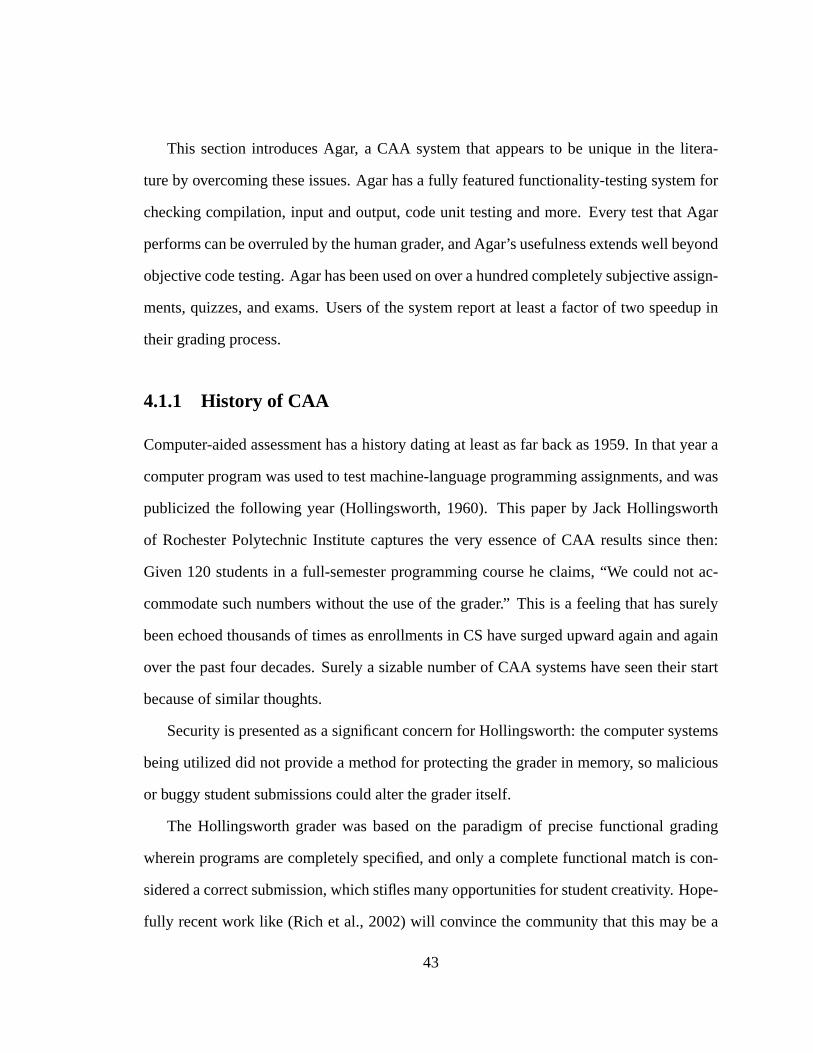
This section introduces Agar, a CAA system that appears to be unique in the litera-
ture by overcoming these issues. Agar has a fully featured functionality-testing system for
checking compilation, input and output, code unit testing and more. Every test that Agar
performs can be overruled by the human grader, and Agar’s usefulness extends well beyond
objective code testing. Agar has been used on over a hundred completely subjective assign-
ments, quizzes, and exams. Users of the system report at least a factor of two speedup in
their grading process.
4.1.1 History of CAA
Computer-aided assessment has a history dating at least as far back as 1959. In that year a
computer program was used to test machine-language programming assignments, and was
publicized the following year (Hollingsworth, 1960). This paper by Jack Hollingsworth
of Rochester Polytechnic Institute captures the very essence of CAA results since then:
Given 120 students in a full-semester programming course he claims, “We could not ac-
commodate such numbers without the use of the grader.” This is a feeling that has surely
been echoed thousands of times as enrollments in CS have surged upward again and again
over the past four decades. Surely a sizable number of CAA systems have seen their start
because of similar thoughts.
Security is presented as a significant concern for Hollingsworth: the computer systems
being utilized did not provide a method for protecting the grader in memory, so malicious
or buggy student submissions could alter the grader itself.
The Hollingsworth grader was based on the paradigm of precise functional grading
wherein programs are completely specified, and only a complete functional match is con-
sidered a correct submission, which stifles many opportunities for student creativity. Hope-
fully recent work like (Rich et al., 2002) will convince the community that this may be a
43

good paradigm to practice from time to time to ensure students are capable of following
directions, but to attract a more diverse population and keep retention high, we must allow
for more creativity.
However, this theme of I/O-spec grading continues through most or all of the CAA
systems in the literature. In the late 1960s, the breakthrough CAA system was the Basser
Automatic Grading Scheme (BAGS) (Hext and Winings, 1969) from the University of
Sydney, which represented the first time that a grader could be used without special support
from a human operator. The paper describing BAGS makes it quite clear what types of
programs are acceptable for grading: precise mathematical operations with zero creativity
or margin for error.
More recently, the mid- 1990s saw the development and publication of systems like
Kassandra (von Matt, 1994), an automated grading system designed for a scientific com-
puting course to evaluate Maple or Matlab code. Kassandra is a system with a number of
very impressive features, like networked operation and a secure client-server paradigm that
absolutely prevents students from interacting with the reference solutions. Especially in the
face of growing sophistication on the part of the students, Kassandra certainly represents a
step in the right direction: who hasn’t worried at some point about compiling and running
student code, either with the use of a CAA tool or even just by hand? Still, we find that
Kassandra focuses exclusively on grading precise functional behavior, and little more.
Based on the published literature it is difficult or impossible to evaluate the usability
of the system. A fundamental concept in human-computer interaction is that programs
are difficult to use if the system model doesn’t match with the user model (Tognazzini,
1996). Since users generally come to a new program with little or no initial concept of the
precise workings of the system, user model is often wildly erratic, at least during the initial
stages of use. Users experience a great deal of stress when they are suffering from such
44

a model mismatch. A reliable method for reducing the time necessary to correct the user
model is to leverage existing, known usage patterns. In essence, the system model should
match existing usage patterns as much as possible so that a user doesn’t have to deal with
expectation violations that cause a program to be “hard to use.” Without having actually
interacted with these other CAA systems, we cannot judge for certain whether the program
matches existing grading styles, but there doesn’t appear to be much reason to assume that
this sort of usability was of much import to the designers of these systems.
4.1.2 Agar
Agar attempts to be a highly usable tool by focusing on the following design principles:
1. Allow existing grading styles - Both in terms of how an individual grader grades, and
how grading tasks are broken up for large classes, Agar attempts to match existing
grading styles.
2. Support the subjective - Agar goes beyond most CAA systems by supporting grading
of subjective features (style, documentation, written work), rather than just function-
ality. This means it can be used for tests and quizzes, or programming work with a
creative aspect.
3. Eliminate repetition - Whenever possible, Agar eliminates the repetitive tasks in
grading. One of the primary ways it does so is by making student feedback instantly
reusable. This trait also applies to recording scores in a gradebook, emailing students
their scores and feedback, and compiling programming submissions.
Grading with Agar can be broken up into five main phases: identifying submission files,
setting up a rubric, running tests and conversions, performing any needed manual grading,
and reporting scores.
45

Identifying Submissions
Our homework-submission system has students turn in an entire directory at once. One
effect of this is that there are often extra files that are not strictly necessary to make a
programming assignment function: object files, backup source files, sample inputs, etc.
Agar includes three main methods of identifying which of the files in a student’s submission
directory are actually part of their submission and should be included in Agar’s list of files
for that student. When we first started working on CAA systems, one of our requirements
was that students submit files with a precise filename. On average, ten to twenty percent of
the students ignored these requirements, regardless of how terrible a penalty was imposed.
Eventually we decided it would be far better for our systems to be able to automatically
identify which files were pertinent.
The default method of identification uses filemasks to identify which files are important.
When starting a new Agar workspace it prompts the user for what kind of grading is to be
done. For written grading, this sets the filemask to*.ps, *.pdf, *.txt, *.doc. Any filename
in the submission directory matchinganyof those Unix-style globs will automatically be
included in the student’s file list. Similarly for C/C++ grading, the filemask is set to*.c,
*.cc, *.cpp, *.h, *.hh, Makefile. This covers the majority of our grading, but an option
exists to manually enter an arbitrary filemask as well. Once the filemask is identified, a base
directory is selected. It is assumed that this directory contains student submissions in the
format generated by ourturnin system (this can be easily altered for other environments).
For each submission directory, the filemask is applied and a collection of matching files
are extracted. If no files match the filemask in one or more directories, then the user is
prompted to manually identify submission files for those submissions.
Another method of identifying files relies on the student submitting a valid (but simple)
Makefile. For each dependency in the Makefile that doesnot have an associated creation
46
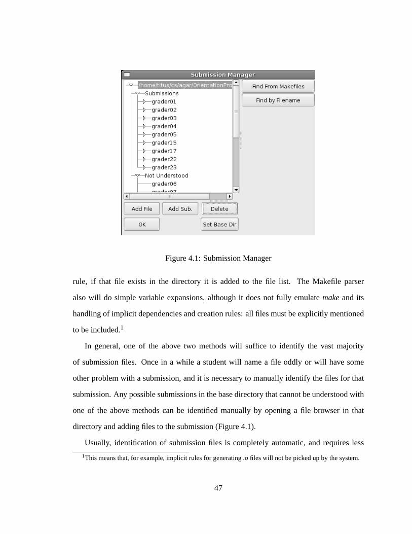
Figure 4.1: Submission Manager
rule, if that file exists in the directory it is added to the file list. The Makefile parser
also will do simple variable expansions, although it does not fully emulatemakeand its
handling of implicit dependencies and creation rules: all files must be explicitly mentioned
to be included.1
In general, one of the above two methods will suffice to identify the vast majority
of submission files. Once in a while a student will name a file oddly or will have some
other problem with a submission, and it is necessary to manually identify the files for that
submission. Any possible submissions in the base directory that cannot be understood with
one of the above methods can be identified manually by opening a file browser in that
directory and adding files to the submission (Figure4.1).
Usually, identification of submission files is completely automatic, and requires less
1This means that, for example, implicit rules for generating.o files will not be picked up by the system.
47

than five minutes for a class of forty students, even in the presence of submissions whose
files were not named correctly or located in the expected locations.
Creating a Rubric
Once submission files are identified, the next step is to create the basic grading rubric. In
Agar, a rubric is a tree of tests. The top-level items are the point categories that will be
reported for student grades. For programming work these are often one major functional
category (“Insert”, “Remove”, “Style”, etc); for written work there is generally a top-level
rubric item for each question. Each rubric item is selected from the available set of tests
(the left portion of Figure4.2). If a rubric item fails, any sub-tests of that item will be exe-
cuted, allowing for conditional execution when necessary. The most common usage of this
hierarchical testing thus far is for compilation: in our department we generally require the
g++ flags-W -Wall -Werror -pedanticfor lower-division programming courses. This helps
ensure that the students are writing good code. Often there will be a mandatory penalty
for code that fails to compile with these flags: by allocating some rubric points to the de-
fault “Compile” (with flags), and then creating a sub-test that re-attempts the compilation
without the flags, we can quickly compile all submissions that are compilable as well as
identify which students had warnings in their code.
Most of the tests shown in Figure4.2 are separate executable programs adhering to
the Agar tool specification. With very few basic requirements on parameter parsing and
exit codes, Agar users can write their own programs and scripts to perform testing tasks
in Agar. The tool specification is quite minimal, requiring on the order of tens of lines
of code, and eliminates the need for a complex plugin structure, dynamic linking, shared-
object generation, or any other complex scheme. Anybody should be able to easily write
extensions for Agar, in any language, so long as that language can read command line
48
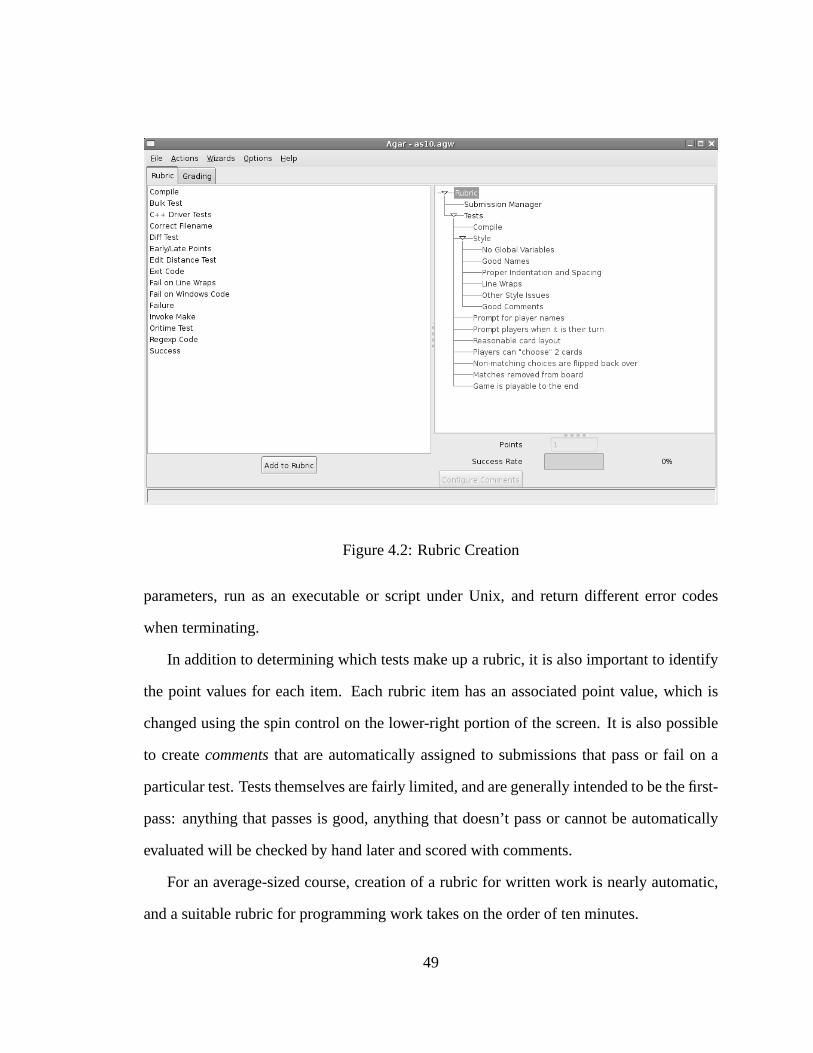
Figure 4.2: Rubric Creation
parameters, run as an executable or script under Unix, and return different error codes
when terminating.
In addition to determining which tests make up a rubric, it is also important to identify
the point values for each item. Each rubric item has an associated point value, which is
changed using the spin control on the lower-right portion of the screen. It is also possible
to createcommentsthat are automatically assigned to submissions that pass or fail on a
particular test. Tests themselves are fairly limited, and are generally intended to be the first-
pass: anything that passes is good, anything that doesn’t pass or cannot be automatically
evaluated will be checked by hand later and scored with comments.
For an average-sized course, creation of a rubric for written work is nearly automatic,
and a suitable rubric for programming work takes on the order of ten minutes.
49
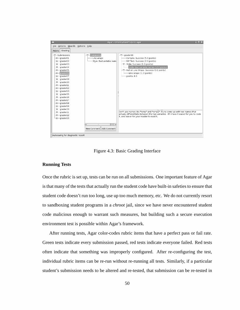
Figure 4.3: Basic Grading Interface
Running Tests
Once the rubric is set up, tests can be run on all submissions. One important feature of Agar
is that many of the tests that actually run the student code have built-in safeties to ensure that
student code doesn’t run too long, use up too much memory, etc. We do not currently resort
to sandboxing student programs in achroot jail, since we have never encountered student
code malicious enough to warrant such measures, but building such a secure execution
environment test is possible within Agar’s framework.
After running tests, Agar color-codes rubric items that have a perfect pass or fail rate.
Green tests indicate every submission passed, red tests indicate everyone failed. Red tests
often indicate that something was improperly configured. After re-configuring the test,
individual rubric items can be re-run without re-running all tests. Similarly, if a particular
student’s submission needs to be altered and re-tested, that submission can be re-tested in
50
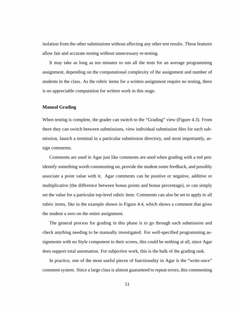
isolation from the other submissions without affecting any other test results. These features
allow fair and accurate testing without unnecessary re-testing.
It may take as long as ten minutes to run all the tests for an average programming
assignment, depending on the computational complexity of the assignment and number of
students in the class. As the rubric items for a written assignment require no testing, there
is no appreciable computation for written work in this stage.
Manual Grading
When testing is complete, the grader can switch to the “Grading” view (Figure4.3). From
there they can switch between submissions, view individual submission files for each sub-
mission, launch a terminal in a particular submission directory, and most importantly, as-
sign comments.
Comments are used in Agar just like comments are used when grading with a red pen:
identify something worth commenting on, provide the student some feedback, and possibly
associate a point value with it. Agar comments can be positive or negative, additive or
multiplicative (the difference between bonus points and bonus percentage), or can simply
set the value for a particular top-level rubric item. Comments can also be set to apply to all
rubric items, like in the example shown in Figure4.4, which shows a comment that gives
the student a zero on the entire assignment.
The general process for grading in this phase is to go through each submission and
check anything needing to be manually investigated. For well-specified programming as-
signments with no Style component to their scores, this could be nothing at all, since Agar
does support total automation. For subjective work, this is the bulk of the grading task.
In practice, one of the most useful pieces of functionality in Agar is the “write-once”
comment system. Since a large class is almost guaranteed to repeat errors, this commenting
51
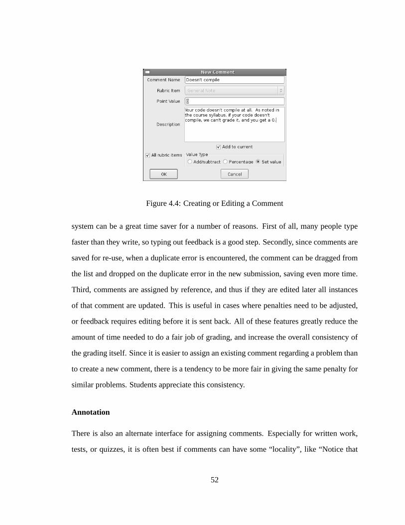
Figure 4.4: Creating or Editing a Comment
system can be a great time saver for a number of reasons. First of all, many people type
faster than they write, so typing out feedback is a good step. Secondly, since comments are
saved for re-use, when a duplicate error is encountered, the comment can be dragged from
the list and dropped on the duplicate error in the new submission, saving even more time.
Third, comments are assigned by reference, and thus if they are edited later all instances
of that comment are updated. This is useful in cases where penalties need to be adjusted,
or feedback requires editing before it is sent back. All of these features greatly reduce the
amount of time needed to do a fair job of grading, and increase the overall consistency of
the grading itself. Since it is easier to assign an existing comment regarding a problem than
to create a new comment, there is a tendency to be more fair in giving the same penalty for
similar problems. Students appreciate this consistency.
Annotation
There is also an alternate interface for assigning comments. Especially for written work,
tests, or quizzes, it is often best if comments can have some “locality”, like “Notice that
52
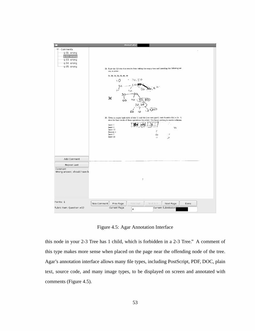
Figure 4.5: Agar Annotation Interface
this node in your 2-3 Tree has 1 child, which is forbidden in a 2-3 Tree.” A comment of
this type makes more sense when placed on the page near the offending node of the tree.
Agar’s annotation interface allows many file types, including PostScript, PDF, DOC, plain
text, source code, and many image types, to be displayed on screen and annotated with
comments (Figure4.5).
53
Using the annotation interface allows graders to grade either submission by submission
or question by question (especially useful for scanned tests where all questions are on
the same page of the submission). When mailbacks are generated for students, all of the
“pages” of their submission are converted to PDF, and the localized comments are added
to the PDF as annotations viewable within Adobe Acrobat Reader2 as colored sticky-notes
that expand to hold the comment text.
Reporting Scores
When the manual grading is completed, the remaining tasks are to generate feedback for
the students and to record scores in the course gradebook. Generating feedback for the
students is easy, assuming the students all have email addresses in the same domain. Agar
identifies student submissions by their username, and can be configured with an outgoing
SMTP server and the domain of the students. It then generates mailback files containing
score summaries, test results, and comment feedback. If the annotation system was used it
also converts the submission to PDF and annotates it with the appropriate comments. When
the mailbacks have all been generated, it automatically emails them out to the students.
For exporting grades, Agar primarily supports the use of a spreadsheet for storing
grades. It prompts for the location of the course gradesheet, which can be in either Mi-
crosoft Excel format or the open-source Gnumeric format. It then searches the gradebook
for a sheet called “Summary” which has a listing of the student usernames. Based on the
row-ordering of those usernames, it creates a new sheet with the scores for the current as-
signment, with one column for each top-level rubric item and with students ordered into the
same row order in the new sheet as they appear on the Summary sheet. It also (optionally)
will export a column of indirect-references to the total points column of the Summary sheet
2Most other PDF viewers ignore annotation information.
54

to keep it up to date. Not only does use of Agar obviate hand entry of score data, it also
allows scores to be recorded and tracked at a much finer granularity than would otherwise
be kept. This detailed data forms the basis of much of our EDM analysis.
4.1.3 Usage Patterns
Two relatively simple features of Agar that have been found to be quite powerful are the
ability to save different portions of the workspace into different files, and to merge Agar
files together. These abilities allow for usage patterns similar to those that are normally
found in courses with large grading loads.
One feature that has been used repeatedly is that of the pre-developed rubric template.
The Head TA for a large class generally creates a rubric and a default set of expected
comments. The Head TA will then save just the rubric and comments into a “template”
file that is given to the other TAs along with a list of which students to grade. Each TA
runs Agar on their own set of submissions, grades using that rubric and those comments for
even greater consistency, and then sends back an Agar workspace complete with grading
information. The Head TA merges all of these Agar workspaces together before sending
mailbacks and exporting grades. This is a simple method of splitting the workload student-
by-student. After grading, the templates can be updated with the most common problems
not covered with the original comments, and saved for use in future course offerings.
When grading exams for large courses, Agar also allows the work to be split question-
by-question. Again, a Head TA creates a rubric and possibly some basic comments for
each question, and then gives a copy of the full workspace (with all rubric information
and student submissions) to each TA, along with instructions for which question to grade.
The TAs grade in parallel, just as they would with paper grading, and then send their Agar
workspaces back for merging. While the selective saving and merge abilities of Agar are
55

not technically complex, they have proven to be invaluable in the adoption of the system,
quickly becoming one of the most-used features.
4.1.4 Conclusions
Agar is, as far as we can tell, a first-of-its-kind entry into the domain of CAA tools. Agar
embraces the idea that feedback from a human grader is an essential and invaluable part of
the learning process. Rather than strive only for complete automation, Agar works to extend
the existing usage patterns of graders by emulating red-pen grading as well as division-of-
labor methods for large grading tasks. By automating the tasks of score recording and
sending feedback to students, Agar works to eliminate the clerical tasks that can otherwise
take up so much time in grading. The “write-once” comment system also makes grading
in Agar more consistent, and allows graders to increase the quality of feedback to students.
Agar is more than just an automated grading system: it is an actualaid for assessment, not
a replacement for the feedback and expertise that is so critical in the learning process.
4.2 HOMR
Optical Mark Recognition, fill-in-the-bubble, multiple-choice tests have been a staple of
educators for decades. The most common approach to OMR for educational institutions
involves specialized reading equipment and preprinted forms, and often lacks important
features such as error checking and digital recording of scores. There are number of com-
mercial OMR software packages (Open Directory, 2005) that allow the use of general-
purpose sheet scanners and self-printed forms, but they do not seem to have achieved ma-
jor penetration into the academic market. Our system, affectionately named the Homebrew
56

Optical Mark Recognition system (HOMR), is an attempt to remedy the lack of a conve-
nient open-source alternative.
HOMR is fully configurable, with certain basic requirements, and allows the authors of
tests, quizzes, surveys, or grade reporting forms to design forms to their own specifications
and to process the images generated by (increasingly cheap and common) autofeed sheet
scanner. HOMR is designed to be highly cross platform, and easily embedded into the
high-level language of your choice. During our testing of the system, we have achieved
maximum accuracy rates of greater than 99.992%: fewer than 80 errors per million bubbles.
For comparison, the OMR system used by the US Census has an estimated accuracy of
99.8% (Bureau, 2004), or 2000 errors per million.
This section describes the requirements for installation and usage of HOMR, the work-
ings of the system itself, and our testing and evaluation methods.
4.2.1 Requirements
HOMR has relatively few requirements. Pages should be bounded with a rectangular bor-
der, and bubbles should be arranged in rectangular grids (see Figure4.2.1). HOMR has
been tested on numerous scanners, from single-page flatbed scanners3 to modern high-
volume office scanners. Students have been allowed to print their own answer pages for
our mark-recognition system, meaning that hundreds of printers have been used for form
generation, and there are thousands of pairwise combinations of printer and scanner that
have been tested with this system. As a result, we feel that HOMR is both printer and
scanner independent.
To date, the vast majority of testing for HOMR has been done using forms generated
in LATEX, but we have had equivalent success in testing the system on forms generated in
3Which are supported, but not recommended for speed reasons.
57
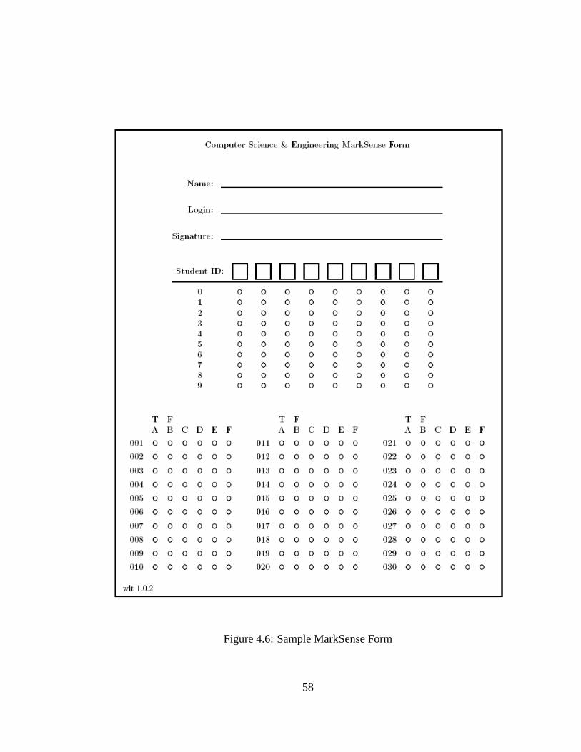
Figure 4.6: Sample MarkSense Form
58

WYSIWYG editors like Microsoft Word or OpenOffice Writer, so there are no require-
ments regarding the method of form preparation. Functionally, the necessity of having a
bounding box and the regular grid layout for bubbles are the only two significant require-
ments, which allows for great flexibility in form creation and layout. For best results, both
printer and scanner must produce good quality, high-contrast results.
4.2.2 Internal Design
HOMR is a small program for the amount of usability power and flexibility it provides.
It requires a single non-standard library, Magick++ (Magick++, 2006), the C++ bindings
to the popular cross-platform open-source graphics library ImageMagick (ImageMagick,
2006). The source for HOMR itself relatively small, comprised of approximately 1200
lines of C++ code. This code performs all of the image normalization, feature detection,
sampling, and bubble classification for HOMR.
Image Normalization
The image normalization step for HOMR has become a larger and larger collection of
algorithms and tricks to deal with a larger and larger collection of printer and scanner bugs
and eccentricities. For example, if a HOMR page is originally stapled to a test and is
then ripped off, the corner of the page may be physically disconnected. Many scanners will
render this as a black blob in one corner of the image. These blobs can throw off the feature
detection in later steps, so HOMR now performs a white flood-fill in each corner to fill in
any such blobs, or black triangles from slightly rotated pages.
In order to find the page borders of the image, a copy is made in memory and run
through a standard edge enhancement algorithm. The edge enhancer is part of the Mag-
ick++ library, but is just convolving the image with an appropriate kernel. The edge en-
59
hancement step is necessary for pages that were generated on copiers running low on toner.
Such copiers will often leave one or more stripes of lower-intensity black on the image,
which may or may not be scanned correctly by the scanner. Edge enhancement boosts the
contrast of these lines, allowing the next step to be performed correctly.
On the edge-enhanced copy of the image, we now perform a standard Hough trans-
form (Duda and Hart, 1972) to find the numeric parameters of the lines present in the
image. The Hough transform views every filled pixel in the image as a “vote” for every
possible line that could pass through that point. By finding all the filled pixels and finding
all pairs ofr andθ that satisfyr = xsin(θ) + cos(θ), we can find the lines in the Hough
space ofr andθ that have sufficient votes to be considered lines in the image4.
This is a particularly processor intensive step as described. Since the pages being fed
to HOMR are expected to have the bounding box lines within a few degrees of vertical
and horizontal, significant speedup can be provided by only looking forθs within±5◦ of
0◦, 90◦, 180◦ and 270◦. Further, by only sampling every-other pixel (and reducing the
vote threshold by half), equivalent lines should be extracted from the image for half the
processing time. Both of these techniques are used by HOMR speed up the detection of the
bounding box.
In order to determine which set of lines is actually forming the bounding box, HOMR
employs a nearest-neighbor search on the “ideal” coordinates inr,θ -space for the bounding
box edges. Currently this is an unconnected-search, in that there is no check performed to
make sure that the lines do in fact touch at the corners. A possible refinement to the system
would be to search for boxes similar to the ideal bounding box in a higher dimensionality
space, but the transformation of lines from ther,θ space into boxes in a higher-dimensional
space would be computationally complex. The current system performs very well on a
4Given only integer values ofθ
60

wide variety of inputs, so such refinements are currently considered unnecessary, and likely
would cause a significant speed penalty.
Given the parameterization of the lines for the bounding box, HOMR now returns to the
copy of the image without edge detection. Given the bounding box lines, the rotation and
skew of the image is calculated. An affine transformation is applied to the image to remove
rotation and skew caused by the printing or scanning of the page. The page is cropped on
the margins. At this point, the page is straight, deskewed, and the image is made up only
of the portion of the scan within the bounding box. A slight Gaussian blur is now applied
to the image to reduce noise and spread the color values more evenly, and then the image is
quantized down to two colors (roughly black and white) to minimize the effect of varying
brightness and contrast scanner settings.
Sampling
At this point the page is prepared for bubble extraction and classification. The configuration
file is read to get the description of each of the bubble arrays on the page. The configuration
file provides the position of each bubble arrayas a percentage of the width and height of
the bounding box, as well as the number of rows and columns present in the array. This
avoids the possibility of scaling changes brought about by various printers and scanners.
The processing of each bubble array begins by looping through the described area of the
page. Thex andy coordinates of each filled pixel are added to an array ofx values and
a separate array ofy values. In order to determine the precisex andy values of the rows
and columns, these arrays are passed to a one-dimensionalk-means clustering algorithm,
given the number of rows and columns to extract. The clusters returned identify thex and
y values of the rows and columns of bubbles, allowing independent location of each bubble
center and sampling of each bubble.
61

Bubbles are extracted by finding the extent of adjacent filled pixels. Starting at the
x,y coordinate given by the grid clustering, the nearest filled pixel in each cardinal direc-
tion is identified, and the extent of filled pixels reachable from those points is identified.
It is necessary to start from several points to account for the possibility of noise in the
center of an unfilled bubble. This is a particularly common condition in the presence of
incompletely-erased bubbles. The reachability search is limited in how far from the origi-
nal x,y coordinate it can search, to prevent sampling too large an area in the case of extra
lines through the page (a common problem with some scanners.) Once the extent of the
connected area is found, a 10×10 sample is extracted. Several extra features are added to
this sample, including the average darkness of the sample, and the width and height ratio.
Once all the bubbles are extracted, the most important feature is added to the samples: the
relative darkness. Each bubble is ranked on a scale of 0..1, with 0 being the darkest bubble
in the array, and 1 being the lightest bubble in the array.
The sample vectors for each bubble are 106 dimensional. These vectors are made up of
100 dimensions for the 10×10 sample itself, and 6 additional features about the bubble,
described below.
• Average pixel intensity in the sample
• Width of the sample as a percentage of page width
• Height of the sample as a percentage of page height
• The product of the width and height values above
• A guess of the correct label (filled or unfilled) based on nearest-neighbor classifica-
tion against three “ideal” bubbles (one filled, one empty, and one crossed out).
62
• A value in 0..1 representing how dark this sample is compared to other samples in
this array. Thus, the lightest bubble in the array is 0, the darkest is 1, and a bubble
only 1% lighter than the darkest is 0.99.
Once the samples are extracted, they may be classified. Classification uses a boost-
ing (Freund and Shapire, 1997) classifier trained on 170 pages of HOMR bubbles (ap-
proximately 11000 bubbles) and generated using the Weka framework (Witten and Frank,
2005). The classifier is made up of 25 decision stumps, ranging in weight from 6.77 to 1.2
(meaning that the most important voters in the classifier has as about 3 times the weight
of the least-important voter). The classification problem is simple: each bubble is to be
reported as either filled or unfilled. In the current classifier, the most important single fea-
ture by far is the final feature encoding relative darkness of the sample. This makes good
intuitive sense: the darkest samples are most likely to be filled. Even crossed-out samples
should be lighter, as the added area of the sample (due to the bars extending out of the
bubble) increase the relative amount of unfilled pixels. The width and height product is
also used, but has less weight than several individual features in the image sample itself.
The twenty-five decision stumps used as the base classifiers utilize a total of thirteen of the
available features.
Based on the results from the boosting classifier each sampled bubble is reduced to
a 0 or 1, and reported to standard output in that form. There are two options in use for
this reporting. The first is a raw best-guess output, wherein each bubble is reported as 0
if it has a negative vote and 1 otherwise. The second utilizes semantic knowledge of the
page, in the form of a guarantee: there is exactly one bubble filled in each row (or column,
depending on the array configuration). In this form, the bubble with the highest vote in
the row or column is output as a 1, and all the other bubbles are output as 0. The best-
guess version has bubble classification accuracy greater than 99.9%. The only-one-bubble
63

version has bubble classification accuracy greater than 99.992%. Errors in the only-one-
bubble system are exceptional cases, such as spurious horizontal lines drawn through a
row, or students scribbling out multiple bubbles in a row and pencilling in the letter of their
preferred answer.
4.2.3 Usage
To use HOMR, it is of course first necessary to assemble the form that you will be using.
Our recommendation is to use LATEX, since it allows for easy automation when changing
title and course information, but as mentioned earlier that is not necessary. Once a form
has been generated according to the page layout requirements, a sample should be printed
and scanned. The user will then load the scan into HOMRConf, a simple GUI that helps
generate HOMR configuration files (Figure4.2.3).
HOMRConf is very simple, and cross-platform. It accepts an image-file format, and
displays that image in a new window. The user then identifies the bounding box and the
bubble grids. For each bubble grid, HOMRConf writes out the location within the bounding
box of the upper-left corner, the width and height of the grid, and the number of rows and
columns of bubbles. HOMRConf then displays what a grid with those parameters would
look like overlayed on the sample page. If this captures the bubbles properly, the user
can accept the configuration and (optionally) add the next grid. Additionally, HOMRConf
needs to know whether each grid should be read in row-major or column-major order.
For MarkSense, our OMR system built on HOMR, a single-page quiz has four grids:
one grid of 9× 10 bubbles for the student ID number, and three grids of 6× 10 for 30
a-f answers. An optional second page has a separate configuration (since it is a different
image layout), and supports an additional 90 bubbles in three columns. Configuration for
64

Figure 4.7: HOMRConf: Generating a configuration for MarkSense
65
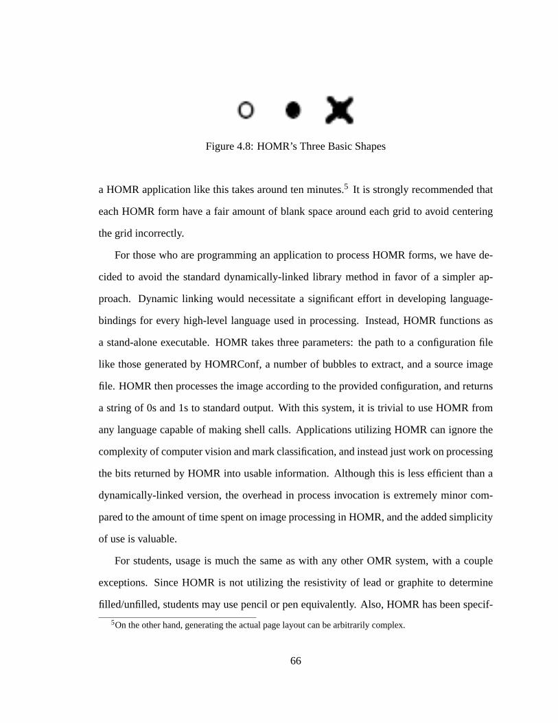
Figure 4.8: HOMR’s Three Basic Shapes
a HOMR application like this takes around ten minutes.5 It is strongly recommended that
each HOMR form have a fair amount of blank space around each grid to avoid centering
the grid incorrectly.
For those who are programming an application to process HOMR forms, we have de-
cided to avoid the standard dynamically-linked library method in favor of a simpler ap-
proach. Dynamic linking would necessitate a significant effort in developing language-
bindings for every high-level language used in processing. Instead, HOMR functions as
a stand-alone executable. HOMR takes three parameters: the path to a configuration file
like those generated by HOMRConf, a number of bubbles to extract, and a source image
file. HOMR then processes the image according to the provided configuration, and returns
a string of 0s and 1s to standard output. With this system, it is trivial to use HOMR from
any language capable of making shell calls. Applications utilizing HOMR can ignore the
complexity of computer vision and mark classification, and instead just work on processing
the bits returned by HOMR into usable information. Although this is less efficient than a
dynamically-linked version, the overhead in process invocation is extremely minor com-
pared to the amount of time spent on image processing in HOMR, and the added simplicity
of use is valuable.
For students, usage is much the same as with any other OMR system, with a couple
exceptions. Since HOMR is not utilizing the resistivity of lead or graphite to determine
filled/unfilled, students may use pencil or pen equivalently. Also, HOMR has been specif-
5On the other hand, generating the actual page layout can be arbitrarily complex.
66

ically trained to identify three primary shapes: empty, filled, and filled-and-crossed-out
(See Figure4.2.3) rather than the common two.6 Filled-and-crossed-out marks count as
empty. Thus, it is generally better for students to cross out an incorrectly filled bubble than
to use a messy eraser or white-out. Also, since HOMR allows size independence for the
bubbles themselves, if the student changes their mindagain after crossing a bubble out,
they can simply make a larger filled bubble, although this level of complexity is generally
not needed.
4.2.4 Testing & Evaluation
HOMR has been utilized on tens of thousands of student submissions, with few user com-
plaints about accuracy. To get more precise accuracy statistics, HOMR was evaluated
on hundreds of real-world student submissions. For evaluation purposes, we compared
HOMR’s results with a human grader’s best guess as to the student’s intended answer,
rather than to whether or not a human would call a given bubble “filled.”
We are currently using a testing dataset of 432 exams from three batches. One batch was
pre-printed and the instructor spent two or three minutes explaining how to fill in bubbles
correctly. Another was the first quiz in a course where students had to bring pre-printed
forms. As a result, the printing quality for this quiz is particularly bad, and students ability
to follow directions is particularly low. The final evaluation batch is the final quiz from that
same course. Many of the same students are present, but now they have some experience
using the system and generally make cleaner marks and better printouts. All told, these
432 submissions contain 74160 bubbles. On these three datasets we achieve accuracy of
6This was an instance of us “giving in” to student usage, since students inevitably crossed out accidentalmarks regardless of our threats to the contrary. As it turns out, specifically allowing crossed-out marks is easyto support, and makes everybody happy.
67

Figure 4.9: A messy bubble grid that is processed perfectly.
68
.99995,.9996, and.9997. The (weighted) average accuracy is.99973, or about 270 errors
per million bubbles. This is significantly more accurate than the U.S. Census, at.998.
However, this level of accuracy is not without a cost. That cost is processing time. On
an AMD Athlon XP 2000+, HOMR takes approximately 17 seconds per page to process
a full-resolution image. This is the setup for which we are providing accuracy numbers
above. For situations in which it is unnecessary to have that much accuracy, or there is
insufficient processing power, there is a simple solution. HOMR does not have strict re-
quirements on the resolution of the input images. The images we use for our MarkSense
application are 8.5×11 inch scanned pages at approximately 150 dpi, but HOMR is gen-
erally able to process the pages at as little as 90 dpi. The processing time is linear in the
number of pixels, so dropping from 150 to 90 dpi gives a speedup of nearly a factor of
three. Even with such a reduced input resolution, HOMR maintains a minimal accuracy
of .999. Below 90 dpi, HOMR has an increasing rate of failure for correctly identifying
the bounding box for the page, thus mis-interpreting entire scans. In practice, we do not
recommend anything below 100 dpi.
4.2.5 Sample Application: MarkSense
The most obvious application for a system like HOMR is for OMR-based grading of
multiple-choice tests. In our department, this application is known as MarkSense. HOMR
evolved out of MarkSense as a generalization of shared code.
MarkSense requires two inputs to function: an answer key, and a PDF collection of the
scanned pages to grade. Command line parameters allow the system to split on any number
of pages per submission and to ignore specified pages.
MarkSense is more powerful than traditional OMR systems in several ways. First, the
answer key format is far more expressive. A basic answer key is made up of a single letter
69

a through f per line in a simple text file. However, MarkSense also allows for arbitrary
combinations of bubbles for answers, a set of alternate answers, as well as different point
scaling for different answers.
Most tests and quizzes in our department follow the normal paradigm of a single cor-
rect bubble. However, we do have instructors that prefer more complex systems. The most
complicated system we regularly see when grading MarkSense quizzes and tests is as fol-
lows: each question is a “mark all that apply,” and for any subset of the correct answer,
the student should get points proportional to the percentage of the correct answers they
provided. Thus if the correct answer is “abd” and the student bubbled “ab”, the student
should receive 2/3 credit. However, if any incorrect bubble is marked, then the student
gets no credit for this question. For a question like this, rather than simply listing “abd” in
the answer key for that line, the answer key format is instead:
abd,ab=.66,ad=.66,bd=.66,a=.33,b=.33,d=.33
This is admittedly somewhat complicated, but this is likely the most complicated system
any department is going to encounter. Again, more standard answer keys are just a single
character per line.
Beyond the added expressiveness of a MarkSense answer key, MarkSense also supports
automated exporting of results to a gradebook. Within our department, the majority of our
gradebooks are stored in Gnumeric (Goldberg, 2006) spreadsheets. MarkSense looks in a
text file mapping 9-digit student ID numbers (given out by the campus registrar) to student
usernames, which can then be found in the course gradebook. Exporting of grades is thus
completely automated with MarkSense. Beyond just exporting totals for each test or quiz,
MarkSense also allows the creation of a new sheet in the spreadsheet with a single column
for each question, and a row for each student. This way we can quickly get per-item student
scores for doing more fine-grained processing of score data.
70

All in all, MarkSense has been a great success in our department. About one in three
courses in our program use MarkSense at least once a quarter, with a nearly ubiquitous
usage for classes of more than a hundred students. Students like it because it allows them
to use pen or pencil, and simply cross out accidental bubbles, to say nothing of avoiding the
cost of purchasing preprinted forms from the campus bookstore. Instructors like it for the
flexibility and automation. Our administrators like it because it means that all MarkSense-
based student quizzes and tests are scanned, and thus readily archived for accreditation.
4.2.6 Conclusions
We have developed a highly-configurable system for Optical Mark Recognition. Using
HOMR, an instructor can easily generate surveys, tests, and quizzes utilizing OMR and
process returned forms using an automatic scanner and standard PC. HOMR allows for
OMR systems with much greater flexibility than traditional OMR systems. For instance,
MarkSense, our first HOMR application, allows for much more complex grading rubrics
for multiple-choice tests than is generally possible with traditional OMR systems. Addi-
tionally, using HOMR allows a completely-digital data path, eliminating the tedious (and
error-prone) process of manually entering grades or survey results. Although it is highly
configurable, HOMR also maintains an accuracy rate higher than the majority of OMR
systems. Most importantly, it is freely available under an Open Source license.
71

Chapter 5
Data Archiving
Compared to collection or analysis, the archiving phase of an educational data mining
project is certainly less critical. If collection is poorly planned or executed, important
data may not be recorded. Improperly executed analysis may prevent pattern discovery, or
worse, cause incorrect or spurious conclusions to be drawn from the data. Poorly executed
archiving should at worst lead to wasted storage space, poor searchability, and inefficient
lookup of the data. Given that the common data sizes in the EDM community are many
orders of magnitude smaller than readily-available storage capacities or processor speeds,
such flaws are hardly fatal. Well archived EDM data can make collection and analysis tasks
easier and more efficient, but a poorly designed storage system will rarely lead to a total
failure of the project, barring catastrophic data loss.
If we hold to the belief that useful and practical EDM projects must minimize human
interaction, the benefits of a well-designed storage system become clear. Just as collection
tools must be built to work with the user and minimize the complexity in recording suffi-
cient data to be useful in an EDM project, archiving can make or break theadoptionof the
system, a different problem than the technical completeness of the system.
72
For most EDM projects, the most obvious method of performing archiving is the now-
ubiquitous SQL database. Although not all ITSes are deployed in a networked environ-
ment, the proportion of ITS installations that do not have access to the Internet is shrinking
as network access becomes ubiquitous in public schools across the country. With off-the-
shelf interfaces into a relational database, there is relatively little complexity in the use of
a database as the storage system for ITS data.
The Marmoset project from the University of Maryland is another example of EDM
storage in a relational database (Spacco et al., 2005). Marmoset archives code snapshots as
students develop programs in Java, along with regular results of unit tests applied to those
snapshots. Utilizing JUnit (Patterson et al., 2003) allows the unit tests to be applied to
individual methods in the assigned Java classes, which allows for very fine-grained testing
and evaluation. For easy numeric EDM analysis, these matrices of unit test results are far
more interesting than the code snapshots, although this code itself may eventually prove to
be a rich data source. According to Spacco, one of the primary researchers on Marmoset,
their database has hundreds of thousands of snapshots, along with the pass/fail results for
about ten unit tests applied to each of those snapshots. Each programming assignment,
and the associated unit tests, generates a different matrix of test results, making these score
matrices on the order of hundreds or thousands of snapshots by ten unit tests. A project of
this scope obviously requires database support, and gains much from the well-developed
query capability and rich user tools associated with modern databases.
Not all EDM data sources can leverage a database. Both the general form of ITS and
the Marmoset project collect data as a side effect of the interface provided to the user. The
program assessment project presented in this dissertation, on the other hand, specifically
must support incremental adoption and instructors who are unwilling to adopt collection
tools like Agar or HOMR. In order to support these kinds of users, we rely on a simpler
73

tool that most instructors are already familiar to our users: the spreadsheet. This provides
much greater robustness and flexibility.
5.0.7 Gradebook Format
In order to facilitate the reporting of scores, we determined early on that it was critical
to make adoption as simple as possible. This is reflected not only in our choice of the
spreadsheet as the grade reporting mechanism of choice, but also in our loose requirements
for formatting of that data.
The format requirements for a spreadsheet in gradebook format to be correctly parsed
by our analysis tools are as follows.
• Summary sheet- We require one page of the gradebook to be named “Summary”,
and to contain at least the following columns:
– ID Column- One column must be named “sid”, “username”, “login”, or “email”
and contain a unique identifier for the students in that row, either their student
ID or their username on our departmental systems.
– Course Grade- One column must be named “Course Grade” and contain the
letter grades assigned to each student.
– Course Score- One column must be named “Course Score” and contain the
numeric score each student earned in the course.
• Instrument sheets- At least one sheet must contain per-item data. There may be
sheets other than Summary and the Instrument sheets. Instrument sheets are identi-
fied by having the following:
74
– ID Column- One column named “sid”, “username”, “login”, or “email”, which
can be mapped to the roster of students on the Summary sheet.
– Relevance data- Instructorsmayprovide the relevance matrixR for the ques-
tions listed on this sheet by adding extra (non-student) rows with “objective1”,
“objective2” . . . “objectiveN” in the ID column and relevance entries in the ap-
propriate rows.
Instructors are allowed to provide gradebook spreadsheets in either the standard Mi-
crosoft Excel format, or the XML-based format for the open-source Gnumeric spreadsheet
package, as well as some lesser-known formats. Script-based extraction and conversion to
standard forms is done by converting to Gnumeric with the Gnumeric utilityssconvert. The
Gnumeric format is merely compressed XML, allowing for rapid development of reusable
tools for manipulating spreadsheet data. By providing loose requirements for instructors
to record grades, we have greatly expanded the adoption of our system. We have also
encouraged the submission of gradebooks by causing our departmentally-approved grade
publishing interface to automatically archive the gradebook storing the grades.
5.0.8 GnumeriPy
After gradebooks are submitted and converted into a standard format, it is important to
develop software methods to allow for easy programmatic manipulation of the data. With
an database interface, this would be SQL. Although the development of an SQL interface
for a spreadsheet backend is an interesting possibility, this was thought to be too much
effort for too little reward. Instead, the functionality that was developed is a Python class
calledGnumeriPy.
75
GnumeriPy operates on spreadsheets and provides the a set of common features ex-
pected for such a tool: saving and loading, exporting a sheet as a CSV flat-file, and basic
data manipulation. GnumeriPy does not parse the full Gnumeric formula syntax, but rather
gives users two modes of interacting with each sheet: raw or frozen. In raw mode, for-
mula cells are stored with the full text string for the formula. This may be edited and
re-stored, but is essentially just a text string. Altering other cells, inserting or deleting rows
and columns, and other spreadsheet operations that could affect the definition of a formula
are ignored. While this provides rather limited functionality, the intended purpose of raw
mode is to work around the formulas or insert new ones. For all the applications in this
dissertation, this has been sufficient functionality. Most collection tools are merely export-
ing grades into existing gradebooks, and thus utilize raw mode, which is sufficient to know
when there are collisions in a cell and prompt for permission to overwrite.
In frozen mode, which can be applied to a single sheet at a time or to the entire spread-
sheet, GnumeriPy invokesssconvertto convert sheets to CSV, effectively evaluating all of
the formulas and providing their results. This is primarily utilized by analysis tools when
converting the gradebook into a suitable format for processing as the score matrixS.
The archiving system developed here, encompassing both our loosely-structured grade-
book format and the GnumeriPy class for gradebook manipulation, demonstrates the pos-
sibility of developing quality archiving systems for EDM projects, even when use of a
database is infeasible.
76
Chapter 6
EDM Analysis Notation and Data
Given our data in spreadsheet format, we can extract course matrices for each gradebook
supplied by participating instructors. These gradebooks can be filled in by HOMR, Agar,
or manually, allowing greater flexibility than is found in many academic development
projects. Once provided with the score matrices, the question is, “What assessment in-
formation can be extracted from the score matrix for this course?” The next four chapters
will address EDM analysis techniques developed to answer this question. As these chapters
are all experimenting on the same datasets, it is useful to first describe these commonalities.
6.1 Notation
The EDM analysis experiments presented in this dissertation are take as input thescore
matrix S. Recall thatSis anm×n matrix recording the scores ofmstudents onn questions.
As part of our program assessment project, we are also concerned with generatingR, the
relevance matrix. R is ann× t matrix encoding the relevance of then questions to each of
t topics. Each entry inRshould be in the range[0,1].
77

Probability of Correct Answer vs. Ability (θ)
0
0.2
0.4
0.6
0.8
1
Pcorrect
Pcorrect
−6 −4 −2 0 2 4 6
θθ
Score probabilities
Characteristic Curve
Figure 6.1: Sample IRT Graph
Some of the experiments presented here also involve statistics inspired by Item Re-
sponse Theory (IRT). In standard IRT the probability of a student with abilityθ answering
a question correctly is given by
P(θ) = 1/(1+eα(θ−β )) (6.1)
Recall then thatβ governs the ability level that best splits the students that should answer
incorrectly from those that should answer correctly. The parameterα is thediscrimination
parameter, governing the accuracy with whichβ splits the two groups: a perfectα means
that all students withβ < θ will answer incorrectly, and vice-versa. A hypothetical sample
plot of θ vs.P is shown in Figure6.1. Points in this plot are estimates of the probability a
question will be answered correctly by students with the given ability levelθ .
78
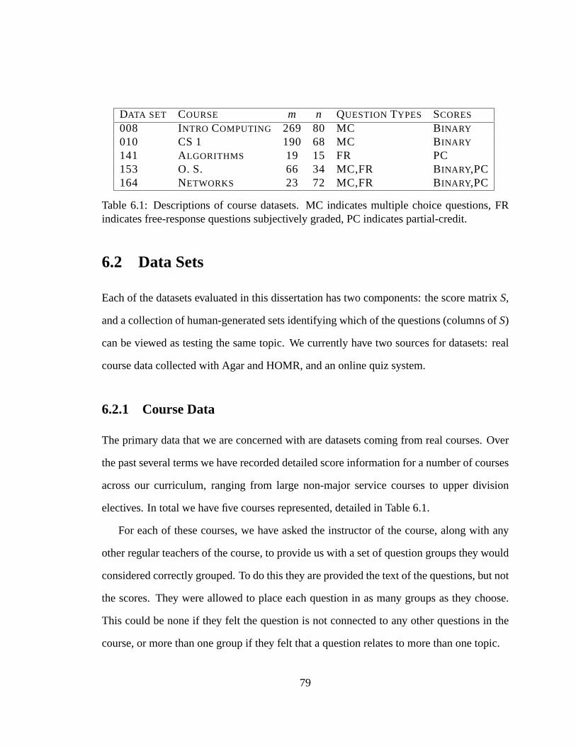
DATA SET COURSE m n QUESTION TYPES SCORES
008 INTRO COMPUTING 269 80 MC BINARY
010 CS 1 190 68 MC BINARY
141 ALGORITHMS 19 15 FR PC153 O. S. 66 34 MC,FR BINARY,PC164 NETWORKS 23 72 MC,FR BINARY,PC
Table 6.1: Descriptions of course datasets. MC indicates multiple choice questions, FRindicates free-response questions subjectively graded, PC indicates partial-credit.
6.2 Data Sets
Each of the datasets evaluated in this dissertation has two components: the score matrixS,
and a collection of human-generated sets identifying which of the questions (columns ofS)
can be viewed as testing the same topic. We currently have two sources for datasets: real
course data collected with Agar and HOMR, and an online quiz system.
6.2.1 Course Data
The primary data that we are concerned with are datasets coming from real courses. Over
the past several terms we have recorded detailed score information for a number of courses
across our curriculum, ranging from large non-major service courses to upper division
electives. In total we have five courses represented, detailed in Table6.1.
For each of these courses, we have asked the instructor of the course, along with any
other regular teachers of the course, to provide us with a set of question groups they would
considered correctly grouped. To do this they are provided the text of the questions, but not
the scores. They were allowed to place each question in as many groups as they choose.
This could be none if they felt the question is not connected to any other questions in the
course, or more than one group if they felt that a question relates to more than one topic.
79
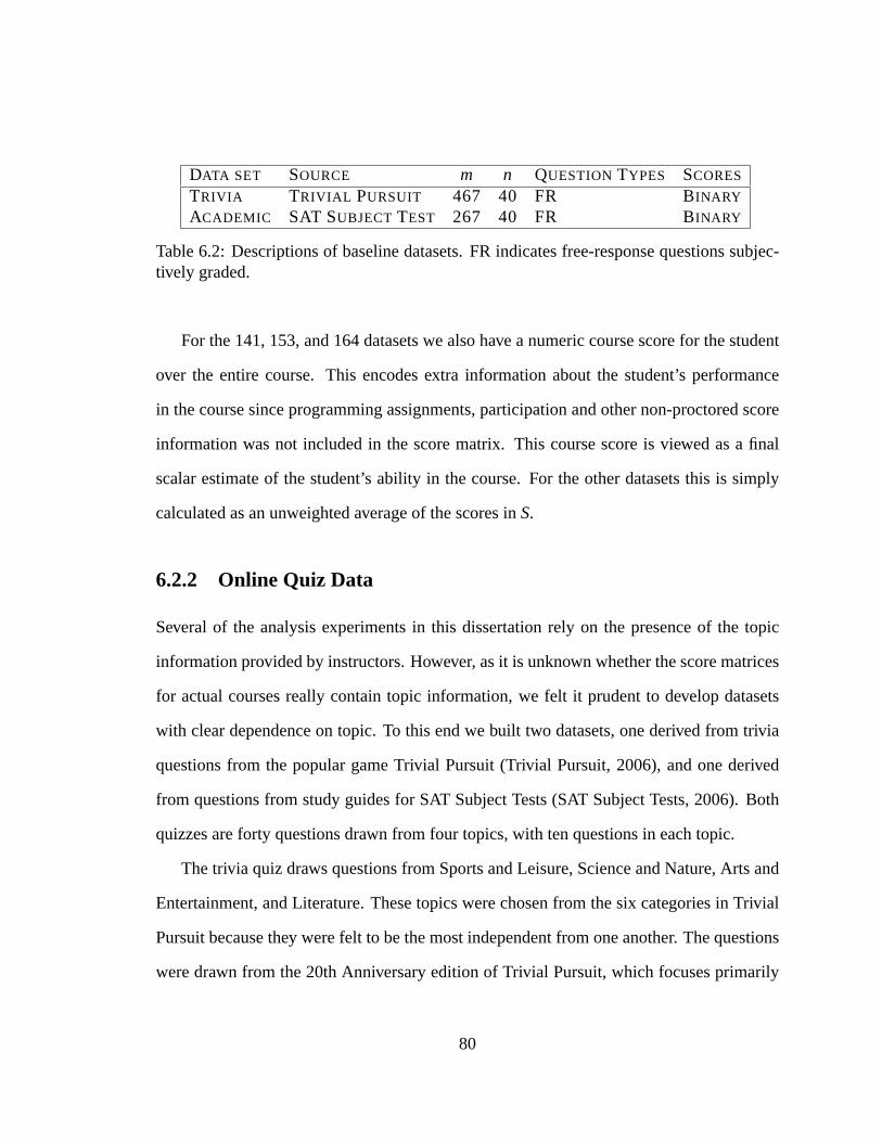
DATA SET SOURCE m n QUESTION TYPES SCORES
TRIVIA TRIVIAL PURSUIT 467 40 FR BINARY
ACADEMIC SAT SUBJECTTEST 267 40 FR BINARY
Table 6.2: Descriptions of baseline datasets. FR indicates free-response questions subjec-tively graded.
For the 141, 153, and 164 datasets we also have a numeric course score for the student
over the entire course. This encodes extra information about the student’s performance
in the course since programming assignments, participation and other non-proctored score
information was not included in the score matrix. This course score is viewed as a final
scalar estimate of the student’s ability in the course. For the other datasets this is simply
calculated as an unweighted average of the scores inS.
6.2.2 Online Quiz Data
Several of the analysis experiments in this dissertation rely on the presence of the topic
information provided by instructors. However, as it is unknown whether the score matrices
for actual courses really contain topic information, we felt it prudent to develop datasets
with clear dependence on topic. To this end we built two datasets, one derived from trivia
questions from the popular game Trivial Pursuit (Trivial Pursuit, 2006), and one derived
from questions from study guides for SAT Subject Tests (SAT Subject Tests, 2006). Both
quizzes are forty questions drawn from four topics, with ten questions in each topic.
The trivia quiz draws questions from Sports and Leisure, Science and Nature, Arts and
Entertainment, and Literature. These topics were chosen from the six categories in Trivial
Pursuit because they were felt to be the most independent from one another. The questions
were drawn from the 20th Anniversary edition of Trivial Pursuit, which focuses primarily
80
on the 1980s and 1990s. As our target audience for the quiz was college students, we
felt this was more likely to result in correct answers than questions from other editions.
Additionally, we chose only questions that had short one or two word answers, as the
online quiz system we developed is a free response system and we wanted to minimize
issues stemming from poor spelling.
The academic quiz draws questions from published study guides for the SAT Subject
Tests. The SAT Subject Tests are taken by students in their final year of high school, and
are used to demonstrate to colleges the depth of knowledge that a student has attained in
particular areas. There are over twenty test subjects available. Again we chose four subjects
that we felt were maximally independent: Math, French, Biology, and World History.
Our assumption was that the trivia quiz could function as a baseline for topic extraction
on data with little or no actual correlation within each topic. Examining the trivia questions,
it is clear that they are indeed trivia: answering any given question correctly is a matter of
isolated fact retrieval, and not a test of any deeper knowledge or skill. As such, even though
there is an obvious “correct” answer when grouping these questions, we did not expect to
be able to extract that answer with any of our candidate algorithms.
The academic quiz represents the opposite end of the spectrum: the questions that were
included come from subjects that are generally studied for at least one academic year in
high school, and possibly several more in college. The questions require a fair depth of
knowledge, and are more topically connected than the trivia questions. Our expectation
was that any algorithm that can succeed in topic clustering will have at least partial success
on this dataset.
The quizzes were administered online over the course of about a week. The trivia quiz
was completed by 467 different visitors, the academic quiz was completed by 267. Cor-
rect answers were immediately reported to the test taker, incorrect answers were reported
81

only as “probably” incorrect. The full text input for any incorrect answers was recorded,
allowing for post-testing processing and correction for unexpected formatting or spelling.
This allowed us to focus on whether the student knew the answer. The two datasets are
summarized in Table6.2.
82
Chapter 7
Question Evaluation
This chapter introduces an assessment mechanism suitable for driving low-level feedback
loops. This answers the questions, “How difficult was question X?” and, “How much do
scores on this question really tell me about what students know?” It can identify questions
that are unintentionally misleading or ambiguous. It produces numeric estimates of the
difficulty and discrimination of a given question, on a known scale for easy comparison.
Most importantly, it is instructor agnostic: this method in no way compares an instructor’s
questions against some theoretical perfect question or a perfect instructor. Questions are
assessed relative to the instructor’s teaching style. Under certain assumptions, we can also
show that these estimates are relatively stable across semesters, allowing more accurate
tests to be generated from banks of existing questions.
7.1 Good Questions
GivenSand the vector of course scores, we can easily evaluate which questions are corre-
lated (in the colloquial sense) with high ability in the course, and estimate the difficulty of
83
each question. We can then begin to learn which types of questions are most meaningful
(have a highα) and which are not. This refinement of questions is based entirely on how
a course is managed, allowing an instructor to know how good a question is with respect
to what the instructor is assessing. Questions that are perfect for one instructor may not be
perfect for another, although it is hoped they are strongly correlated.
The other IRT statistic for each question isβ , the difficulty. Knowingβ for each ques-
tion can grant some insight into what the students are really understanding. Ifβ seems too
high after evaluating a question, it indicates that the topic is not well understood by the
students. Generally, one can assume that a question with a highα and aβ in the useful
range (the range of course scores that would pass the course) is a “good question.”
7.1.1 Calculatingα and β
To see how calculating difficulty and discrimination parameters can be done easily, let
us first assumeβ is known for each question. It is then possible to find the empirical
discriminationα for a question by quantifying how well thatβ separates students that got
the question right from those that got it wrong.
There are a number of ways of calculatingα, and in general they give similar results
in most cases. We have evaluated complex techniques like entropy-based measures, but
in general the simplest technique provides similar results to the more complex techniques.
Our preferred estimate ofα is the fraction of scores that would be guessed correctly under
the assumption that every student with ability underβ got the question wrong and every
other student got it right. For non-binary questions this won’t predict scores correctly, but
does provide an estimate of how well this model matches the data (Figure7.1).
If it really is the case thatβ is a perfect split point, thenα will be 1, a perfect score. If
correct and incorrect scores are evenly distributed on both sides ofβ thenα will be .5, and
84
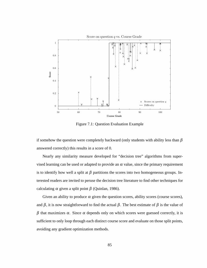
Score on question q vs. Course Grade
0
0.2
0.4
0.6
0.8
1
Score
Score
50 60 70 80 90 100
Course GradeCourse Grade
Scores on question q
Difficulty
Figure 7.1: Question Evaluation Example
if somehow the question were completely backward (only students with ability less thanβ
answered correctly) this results in a score of 0.
Nearly any similarity measure developed for “decision tree” algorithms from super-
vised learning can be used or adapted to provide anα value, since the primary requirement
is to identify how well a split atβ partitions the scores into two homogeneous groups. In-
terested readers are invited to peruse the decision tree literature to find other techniques for
calculatingα given a split pointβ (Quinlan, 1986).
Given an ability to produceα given the question scores, ability scores (course scores),
andβ , it is now straightforward to find the actualβ . The best estimate ofβ is the value of
β that maximizesα. Sinceα depends only on which scores were guessed correctly, it is
sufficient to only loop through each distinct course score and evaluate on those split points,
avoiding any gradient optimization methods.
85

7.1.2 Assumptions
In order for the above method to be usable, several assumptions must be made. First of all,
we are assuming that the question is valid, that is, it has some relevance to the general topic
of the course. Additionally, since nobody can track the true ability level of the students,
the use of course scores is only an estimate. If those scores are highly uncertain (at the
beginning of the course) or have nothing to do with the question, then this is not a valid
assumption. Using course scores implies that each course is a single proficiency. This
is clearly not usually true, but for any course that this is a particularly bad assumption
(for example, a course composed of two half-courses on different topics), it is allowable
to use the scores from only the appropriate portion of the course. It would be ideal to
automatically extract topic information from the score data and track student proficiencies
on a fine-grained level (e.g. ability with linked lists, rather than score in the Data Structures
course), but this remains an area of future work.
The estimates of both parameters rely heavily on the distribution of the course scores.
Student grades fluctuate significantly at the beginning of the course before the law of large
numbers begins to stabilize each student’s grade toward its final value. Therefore, the
values ofα and β are going to be most accurate at the end of the course, and a final
evaluation of which questions are worth keeping for next semester is best done after the
course has completed. It is useful to evaluate questions immediately after grading the
instrument, especially to find topics that were tested but not fully understood, but such
evaluations should be recognized as less-accurate estimates.
Independence of scores is also a concern. If the estimate of ability (course score) in-
cludes the score on the given question, then by definition there is some correlation between
the two. To get the best estimates ofα andβ , it is best to provide ability estimates that do
not include the score on that question or instrument. In practice, if each individual question
86
has a very small effect on the total grade, then this effect is negligible and few questions
need to be evaluated separately.
Finally, it should be pointed out that the course grade may not take into account the dis-
crimination of each question while the course is in progress. If course scores are adjusted to
de-emphasize low-discrimination questions and over-emphasize high-discrimination ques-
tions, then this will make it difficult for anyone to change their overall course standing.
If scores are re-weighted based on discrimination, then a student that initially performed
poorly and studied extra hard would decrease the discrimination on those questions that
they answered correctly due to extra study. A similar argument can be made for good stu-
dents performing poorly at the end of the term. This is a technique for assessing questions,
and the intent is for this to be utilized to make instructors more aware of the questions they
are asking. If this is used to adjust scores, especiallyas the course progresses, early course
grades become more difficult to overcome for students that get off on the wrong foot. As
such, this may be used to perform an initial immediate assessment of the difficulty of the
questions to test for student understanding, but low-discrimination questions should not
be dropped or de-emphasized, and the initialβ values are to be considered an estimate.
Evaluation between offerings will yield more accurate and meaningful statistics.
7.2 Results
This technique was used extensively during Summer 2004 in Introduction to Data Struc-
tures and Algorithms, where it provided very useful feedback to the instructor in question
evaluation. Some of the intuitive insights it confirmed included:
• Do not test on specifics from the text: Questions that test not the subject, but merely a
particular presentation of the subject have little assessment value if that presentation
87

is not a major component of the lecture. Some instructors may choose to explicitly
test this material to encourage students to do the required reading, but that was not
this instructor’s goal. This was demonstrated by a consistently lowα for all questions
testing textbook minutiae rather than the more fundamental concepts.
• Do not test things mentioned in passing: While some may feel that mentioning some-
thing once or twice during lecture is sufficient for the “good” students, this appears
not to be the case. Iterators were discussed as an aside for 10–15 minutes the day
before Quiz 1. This was not nearly enough for even the good students to pick up
the concept. Although 47% of the class answered this question correctly, it is likely
because they narrowed it down to 2 or 3 choices and guessed rather than knowing the
answer, since this question had discrimination of 0.59, implying nearly zero correla-
tion with general course performance.
The most useful feedback this technique provided was in finding questions with unex-
pectedly high difficulties. The most striking example was for the question, “What is the
worst-case time to find an element in a binary search tree ofn nodes?” While there is a
mild “trick” in recognizing that a binary search tree is not necessarily balanced, it was sur-
prising to find that the difficulty score for this question was 87% (with a highα), meaning
that it did a better job of differentiating A’s from B’s than anything else. This was certainly
not intended to be a question splitting the A’s from the B’s. The fact that it was found to
be quite difficult indicated that this aspect of binary search trees was a topic that needed
additional coverage. Since the quiz was graded and evaluated the same day it was issued,
the lesson plan for the next day was altered to account for the fact that the class had missed
this important concept.
88
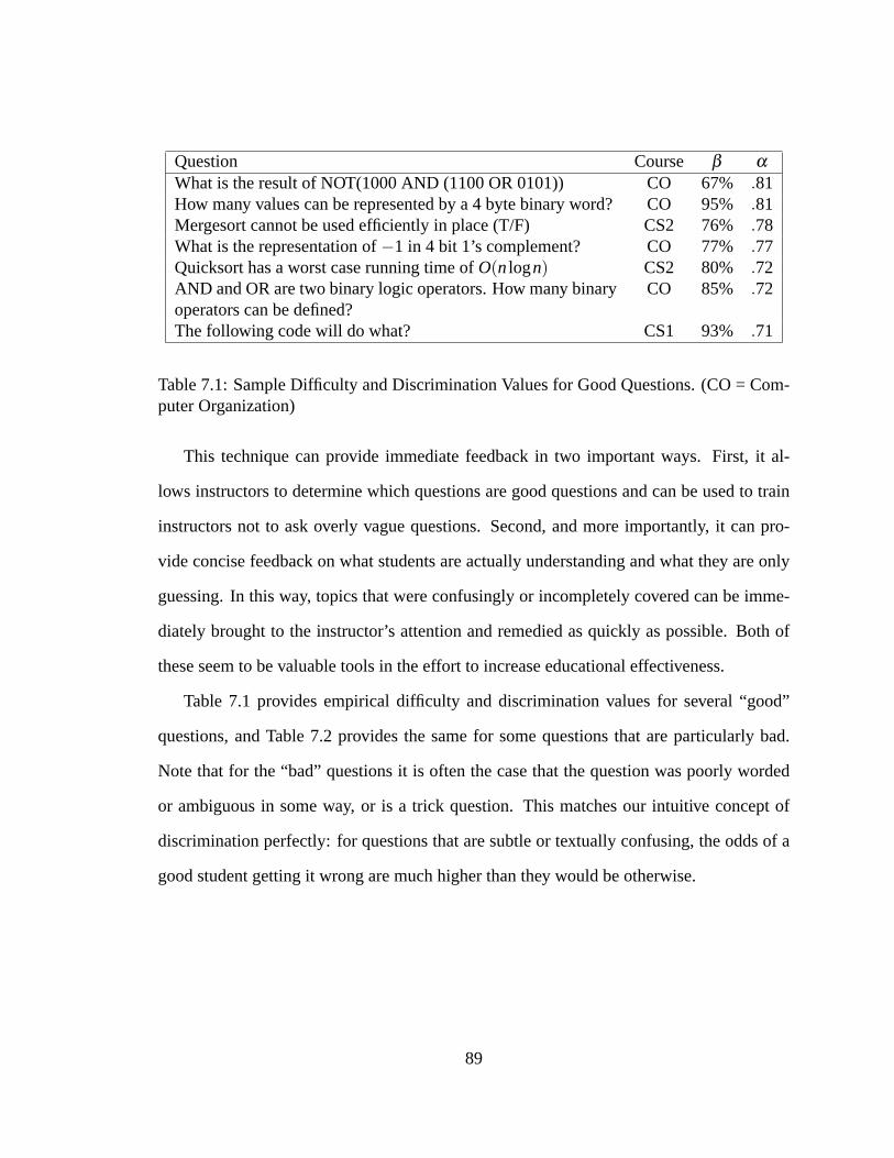
Question Course β α
What is the result of NOT(1000 AND (1100 OR 0101)) CO 67%.81How many values can be represented by a 4 byte binary word? CO 95%.81Mergesort cannot be used efficiently in place (T/F) CS2 76%.78What is the representation of−1 in 4 bit 1’s complement? CO 77%.77Quicksort has a worst case running time ofO(nlogn) CS2 80% .72AND and OR are two binary logic operators. How many binaryoperators can be defined?
CO 85% .72
The following code will do what? CS1 93%.71
Table 7.1: Sample Difficulty and Discrimination Values for Good Questions. (CO = Com-puter Organization)
This technique can provide immediate feedback in two important ways. First, it al-
lows instructors to determine which questions are good questions and can be used to train
instructors not to ask overly vague questions. Second, and more importantly, it can pro-
vide concise feedback on what students are actually understanding and what they are only
guessing. In this way, topics that were confusingly or incompletely covered can be imme-
diately brought to the instructor’s attention and remedied as quickly as possible. Both of
these seem to be valuable tools in the effort to increase educational effectiveness.
Table 7.1 provides empirical difficulty and discrimination values for several “good”
questions, and Table7.2 provides the same for some questions that are particularly bad.
Note that for the “bad” questions it is often the case that the question was poorly worded
or ambiguous in some way, or is a trick question. This matches our intuitive concept of
discrimination perfectly: for questions that are subtle or textually confusing, the odds of a
good student getting it wrong are much higher than they would be otherwise.
89
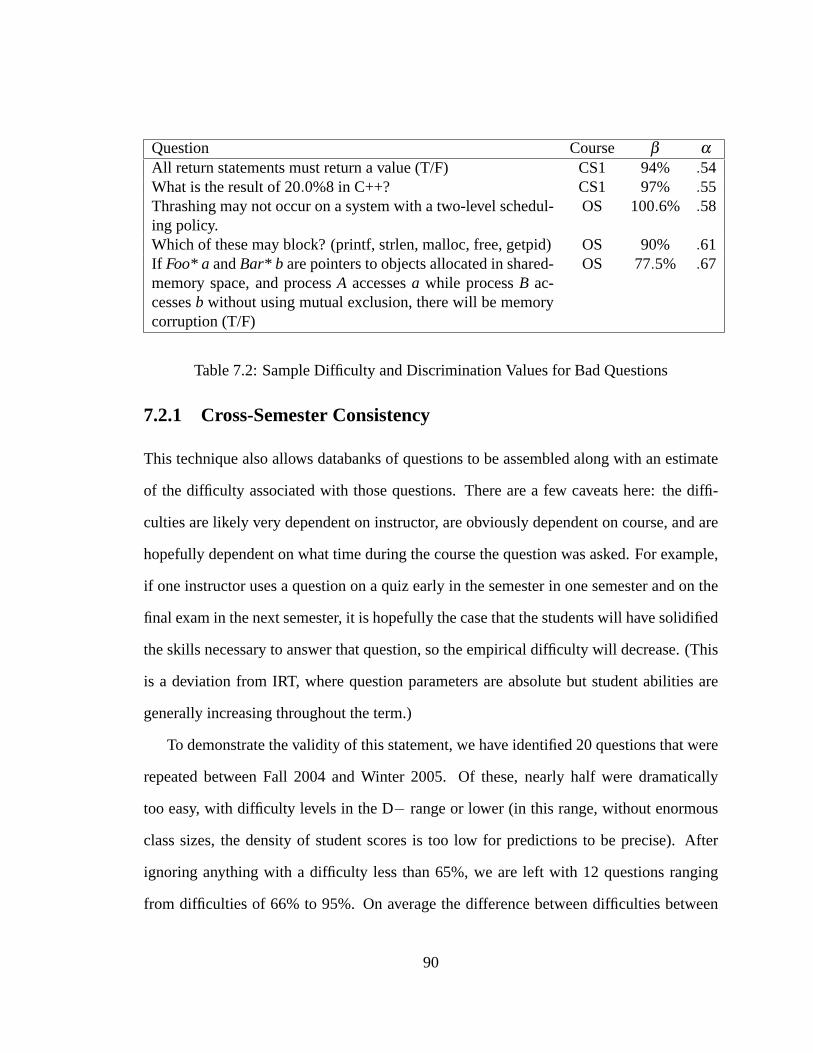
Question Course β α
All return statements must return a value (T/F) CS1 94%.54What is the result of 20.0%8 in C++? CS1 97% .55Thrashing may not occur on a system with a two-level schedul-ing policy.
OS 100.6% .58
Which of these may block? (printf, strlen, malloc, free, getpid) OS 90%.61If Foo* a andBar* b are pointers to objects allocated in shared-memory space, and processA accessesa while processB ac-cessesb without using mutual exclusion, there will be memorycorruption (T/F)
OS 77.5% .67
Table 7.2: Sample Difficulty and Discrimination Values for Bad Questions
7.2.1 Cross-Semester Consistency
This technique also allows databanks of questions to be assembled along with an estimate
of the difficulty associated with those questions. There are a few caveats here: the diffi-
culties are likely very dependent on instructor, are obviously dependent on course, and are
hopefully dependent on what time during the course the question was asked. For example,
if one instructor uses a question on a quiz early in the semester in one semester and on the
final exam in the next semester, it is hopefully the case that the students will have solidified
the skills necessary to answer that question, so the empirical difficulty will decrease. (This
is a deviation from IRT, where question parameters are absolute but student abilities are
generally increasing throughout the term.)
To demonstrate the validity of this statement, we have identified 20 questions that were
repeated between Fall 2004 and Winter 2005. Of these, nearly half were dramatically
too easy, with difficulty levels in the D− range or lower (in this range, without enormous
class sizes, the density of student scores is too low for predictions to be precise). After
ignoring anything with a difficulty less than 65%, we are left with 12 questions ranging
from difficulties of 66% to 95%. On average the difference between difficulties between
90

semesters is 5%, with a standard deviation of 4%, meaning that more than 2/3 of the time,
a repeated question will have a difficulty within one letter grade when used under similar
circumstances.
7.3 Question Evaluation Conclusions
Every student attempt on every question is fundamentally testing two things: the ability of
the student at that point in time, and the quality of the question. In normal teaching, we
evaluate students continuously, and with the aid of the techniques presented here we can
begin to evaluate the questions as well. Evaluating educational effectiveness is an important
concept in current accreditation practices, and we expect that importance to grow in years
to come. The techniques presented in this section provide a simple method to close the loop
on the lowest level of a course feedback process by reinforcing which questions are most
meaningful. Building a catalog of good questions with known difficulties now becomes an
easy task for an instructor. Given the ability to estimate with confidence ahead of time how
difficult a give question is, it is easier to build tests that more accurately assess the students.
Most importantly, a quick analysis of the scores right after administering an exam can
yield immediate feedback to the instructor regarding what topics are being misunderstood,
allowing for quick alterations to the lesson plan to fix misconceptions before they get out
of control. Continuously improving the quality of questions with these techniques is a
low-effort, high-reward strategy that can help all of us.
91
Chapter 8
Predicting Missing Scores
The term Educational Data Mining (EDM) is a bit of a misnomer. In more traditional
fields associated with data mining, like the research published at SIGKDD, the volume
of data present is of such a volume that the running time of the algorithms in question
is of primary concern. Many algorithms presented in the data mining literature are fast
approximations to common machine-learning techniques like SVD or ICA, techniques that
would be difficult or impossible to apply to the volume of data commonly found in the data
mining community. In Educational Data Mining, data volume is generally far lower. EDM
researchers are more likely to have too little data, rather than too much. This is especially
true in research where the data comes from sources other than intelligent tutoring systems
(ITSs), which typically provide data sizes of hundreds or thousands of students on dozens
of problems. In contrast, a typical score matrix for a college-level course involves students
from an average-size class and fewer than 100 questions.
As these smaller datasets become common in EDM research, it will become increas-
ingly important to have complete data in the score matrix. If the score matrix is being
recorded as the scores for each student on each homework or test question across an entire
92
course, then student absences and failure to complete assignments will lead to missing en-
tries in the matrix. Assuming blank entries are zero grossly underestimates student ability,
confusing lack of completion with lack of knowledge. Missing entries are therefore prob-
lematic. Many, if not most, of the algorithms that are being tested in the EDM community
require full data. The options in such cases are few: either discard the scores for every stu-
dent that has at least one missing score, or develop techniques to fill in the missing entries
in the score matrix.
Even in the ITS scenario, score prediction may be a useful practice. Not all students
utilizing a given ITS will necessarily attempt each of the possible questions. In general, the
score matrices from an ITS are likely to be quite sparse, perhaps too sparse for prediction
to be feasible. However, given sufficient density of scores in the score matrix, prediction
may usefully fill in the blank spots.
8.1 Prediction Techniques
In this idealized score prediction experiment we are given a score matrix with a single
missing entry. From the list of valid scores for this question (which we take to be the set of
values seen in this column), we want to predict the missing entry. There are a number of
techniques, ranging from obvious to relatively complex, that are suitable for this problem.
Below are the prediction techniques that were evaluated in this experiment.
8.1.1 Matrix Average (Avg)
The simplest and most naıve technique for score prediction is to calculate the average of
the entire matrix and predict each missing score to be the candidate value closest to that
average. For binary score matrices, this will predict all missing entries identically as 0 or
93

1, depending on the overall average score. This is entirely unsuitable as a real solution for
this problem, but is presented as a strawman: this is the level of predictive performance that
can be attained with essentially zero effort.
8.1.2 Student Average (RowAvg)
A slightly more meaningful technique is to calculate the average score for thestudentand
choose the score that is closest to that average. This assumes that a student’s performance
is relatively constant across questions, and that the ability of the student is more important
than the difficulty of the question.
8.1.3 Question Average (ColAvg)
The converse of the RowAvg technique is to calculate the average score for all students on
this question and predict the value closest to that value. This implies that question difficulty
is more important than student ability, an implication shared with the model for CFA.
8.1.4 Student & Question Average (RowColAvg)
Assigning preference to either student ability or question difficulty seems fairly arbitrary
in the face of exceptional students or exceptional questions. Calculating both the student
average and the question average and averaging those values to select a value for prediction
provides an easy compromise.
8.1.5 Difficulty & Discrimination (DD)
Utilizing the question evaluation technique from the previous chapter, we can extract the
difficulty β for the question using average scores in the matrix as the estimate of overall
94
ability. Note that even for the datasets where an instructor-generated final course score is
present, we are using only the average from the scores inSdue to the possibility of topic
information discussed below. Givenθ as the average of this student on the other questions,
we predict 0 if the student hasθ < β and 0 otherwise.
One significant problem with this approach is that it is only suitable for binary ques-
tions, as it is non-obvious how to expand this to pick from the full list of candidate values.
8.1.6 Conditional Probability (CondProb)
Another method for prediction is to examine the conditional probabilities for each outcome
score based on the known scores in this row or column. For complexity reasons, we can’t do
a full conditional probability based on the joint distribution of scores on the other questions.
However, by looking at the individual distributions of scores on the unknown question given
the scores on each of the other questions independently, we can still make useful predictions
based on estimated conditional probabilities.
More formally: let x be the score in question, andY be the vectory1,y2, . . .yn, this
student’s scores on the othern questions. Given the number of students that we anticipate, it
is not feasible to estimateP(x|Y), since the number of possibilities forY are an exponential
function ofn. However, it is reasonable to estimateP(x|yi) for eachi in 1. . .n, and base our
prediction on those distributions. Experimentally, the best prediction given the collection
of distributions is given by finding the most-often predicted value, which corresponds to the
selecting the maximum likelihood outcome from thesumof the distributions rather than the
more mathematically-grounded product of the distributions. This may be due to the chances
of not seeing a particularx,y pairing, and thus incorrectly estimating one probability as 0,
causing an otherwise good prediction to be ignored completely. This seems likely given
the particularly low performance on smaller datasets. Results for the additive model are
95
presented as CondProb+, and results for the more easily justified multiplicative model are
presented as CondProb×
8.1.7 Noisy OR (N-OR)
A possible explanation for the odd success of the “additive” probability model in the Cond-
Prob algorithm is the “noisy or” model. The N-OR model assumes the probability that
a given score will be correct (set to 1) is related to whetherany conditional probability
feature predicts that it will be correct. The formal model for this is:
p(x = 1) = 1−Πi(1− p(x|yi)) (8.1)
Like the DD algorithm, this only predicts 0 or 1 — specifically it predicts 0 ifp(x =
1)< 0.5, otherwise it predicts 1.
8.1.8 AdaBoost
We have also evaluated the AdaBoost algorithm of Freund and Schapire (Freund and
Shapire, 1997) using a decision stump1 as the base classifier. AdaBoost works by train-
ing a collection of weaker base classifiers on a weighted representation of the training data.
In each round, the training examples that are correctly classified are given reduced weight,
and the remaining examples are given greater weight. The collection of weak classifiers
vote for the correct overall classification, with each classifier given voting weight related to
the accuracy of that weak classifier. After summing the weighted votes, the prediction with
the highest vote is the predicted output.
1A single-question decision tree
96

0
0.2
0.4
0.6
0.8
1
Score
on
Q2
Score
on
Q2
0 0.2 0.4 0.6 0.8 1
Score on Q1Score on Q1
Unknown point
Nearest neighbor
Figure 8.1: Nearest Neighbor Classification Example
8.1.9 Nearest Neighbor (NN)
Nearest neighbor is a quick-and-easy, but respected, technique for classification or predic-
tion. Nearest neighbor stores the data points for which the correct classification is known,
and finds the closest known point, under a particular distance metric, to the point to be clas-
sified. In this application we use the missing column as the labels, and the rows without
missing entries are used as the known classifiers. The non-missing elements of the predic-
tion row are used to calculate the Euclidean distance to each of the classifiers, and the label
of the nearest classifier is used as the prediction. Figure8.1shows an example from the CS
141 dataset, reduced to only two classification dimensions for simplicity.
8.1.10 Topic Information
A final issue to be evaluated in our experiment is the extent to which “topic” information
can boost the predictive ability of the various techniques described above. The questions in
97
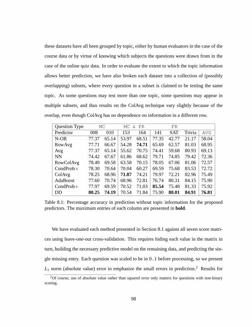
these datasets have all been grouped by topic, either by human evaluators in the case of the
course data or by virtue of knowing which subjects the questions were drawn from in the
case of the online quiz data. In order to evaluate the extent to which the topic information
allows better prediction, we have also broken each dataset into a collection of (possibly
overlapping) subsets, where every question in a subset is claimed to be testing the same
topic. As some questions may test more than one topic, some questions may appear in
multiple subsets, and thus results on the ColAvg technique vary slightly because of the
overlap, even though ColAvg has no dependence on information in a different row.
Question Type MC MC & FR FRPredictor 008 010 153 164 141 SAT Trivia AVGN-OR 77.37 65.14 53.97 68.51 77.35 42.77 21.17 58.04RowAvg 77.71 66.67 54.28 74.71 65.69 62.57 81.03 68.95Avg 77.37 65.14 55.62 70.75 74.41 59.68 80.93 69.13NN 74.42 67.67 61.86 68.62 79.71 74.85 79.42 72.36RowColAvg 78.49 69.58 63.58 70.15 78.05 67.06 81.06 72.57CondProb× 78.30 70.64 70.04 60.27 69.59 75.68 83.53 72.72ColAvg 78.25 68.96 71.87 74.21 79.97 72.21 82.96 75.49AdaBoost 77.60 70.74 68.96 72.81 76.74 80.31 84.15 75.90CondProb+ 77.97 69.59 70.52 71.03 85.54 75.48 81.33 75.92DD 80.25 74.19 70.54 71.84 75.90 80.01 84.91 76.81
Table 8.1: Percentage accuracy in prediction without topic information for the proposedpredictors. The maximum entries of each column are presented inbold.
We have evaluated each method presented in Section8.1against all seven score matri-
ces using leave-one-out cross-validation. This requires hiding each value in the matrix in
turn, building the necessary predictive model on the remaining data, and predicting the sin-
gle missing entry. Each question was scaled to be in 0..1 before processing, so we present
L1 norm (absolute value) error to emphasize the small errors in prediction.2 Results for
2Of course, use of absolute value rather than squared error only matters for questions with non-binaryscoring.
98

Question Type MC MC & FR FRPredictor 008 010 153 164 141 SAT Trivia AVGN-OR 78.41 65.19 59.47 69.19 65.93 53.09 55.07 63.76RowAvg 76.30 62.52 54.28 66.37 74.66 70.81 79.86 69.26NN 73.71 64.83 64.48 70.48 72.78 73.90 73.90 71.02Avg 78.41 65.03 61.16 72.66 75.82 65.59 80.93 71.37RowColAvg 77.00 64.91 63.67 71.73 77.37 71.37 81.22 72.47CondProb× 79.67 70.46 70.99 67.19 67.66 78.59 83.54 74.01ColAvg 79.45 69.51 71.63 75.21 77.17 72.21 82.96 75.45AdaBoost 79.70 71.33 69.77 74.92 72.99 80.57 83.70 76.12DD 82.29 73.34 72.48 75.12 73.34 82.93 84.86 78.02CondProb+ 80.97 77.94 89.56 84.99 95.83 80.77 83.59 84.81
Table 8.2: Prediction accuracy with topic information
prediction without topic information are presented in Table8.1, and results for prediction
with topic information are presented in Table8.2.
In general, two methods stand out in this analysis. For datasets that have not been
pre-split into questions related by topic, the IRT-inspired DD method performs well, and
outperforms any other method investigated on binary data. For datasets that have been re-
duced into questions related by topic, our CondProb+ algorithm significantly outperforms
any other method, and does particularly well on non-binary data. The performance on
partial-credit data makes good intuitive sense, since having a larger number of distinct val-
ues on which to condition the distributions should increase the ability of the CondProb+
technique to differentiate ability levels.
However, it is worth noting that on prediction across multiple topics (that is, when
the score matrix contains questions drawn from more than one topic), the simple ColAvg
predictor performs nearly as well as either the DD method or the conditional classifier. For
the datasets evaluated, the average performance of ColAvg is only 1.3% worse than the DD
method, and within 0.5% of the performance of the conditional classifier. That is, when
99

scores are representing multiple topics, predictingwithout looking at the scores for other
questionsis very nearly as accurate as attempting to build a model to take into account the
full score matrix. The issue of partitioning questions into topic based on the score matrix
is investigated in the next two chapters.
It is also quite interesting that the RowAvg predictor often performs even worse than
predicting based on the overall matrix average, and in almost every experimental case
RowAvg performs worse than ColAvg. If RowAvg prediction were superior, it would imply
that a student’s performance on other questions is more important than the scores of other
students on a particular question. ColAvg outperforms both RowAvg and RowColAvg in-
dicating that the opposite is true: the effect of student ability is dominated by properties of
the question itself. This is in line with previous psychometric models like Common Factor
Analysis (CFA), where the underlying model contains terms for features of the question,
but not for features of the student.
8.2 Educational Use and Implications
Some teachers may be tempted to apply these results to the classroom. Indeed, there are a
few relevant implications that can be drawn. Commonly, when a student misses an assign-
ment or quiz with a valid excuse, instructors face a dilemma: whether to allow the student
to make up the work, or simply to make the instrument “not count,” often by granting credit
equal to the student’s current course percentage, equivalent to the RowAvg method. From
the results shown in Section8.1.10, it is clear that granting credit in this nature is the wrong
solution: if the missed work was particularly easy or particularly hard, it uniformly affected
the grades of the rest of the students, but would not affect the absent student. ColAvg is
more likely to be accurate, but is harder to justify to the student, since their score is com-
100
pletely based on the work of others. The more advanced techniques like DD or CondProb+
are feasible, in that they take into account both the student’s performance and the difficulty
of the individual questions. Whether students will accept a more complex algorithm as the
basis for their score is a subtle social issue, outside the scope of this discussion.
However, it must be noted that this work is preliminary and not yet generalized to
the level of a deployable tool. A side-effect of the leave-one-out validation utilized in
this study is that the predictions can assume thatevery otherentry in the score matrix is
present. Generalizing these techniques to work in the face of numerous missing entries is
not generally difficult, but remains an area of future work. However, there is no obvious
reason that the performance of the techniques investigated here would change dramatically
given properly adapted algorithms.
8.3 Score Prediction Conclusions
Especially when applying new EDM techniques to score matrices coming from classroom
settings, which are most likely producing smaller data sets than do ITS sources, prediction
of missing entries is an important task. Within ITS data sources, accurate prediction may
be necessary before the application of EDM techniques requiring full data, since not all
ITS students will attempt each ITS question. EDM may in fact be more commonly plagued
by missing data than are the data-mining or machine-learning communities.
Accurate prediction of missing entries in score matrices is a problem that depends on
the type of input being provided. If a score matrix represents scores on questions testing
only a single topic, accuracy in prediction rates appear to rise by 5% to 10% over mixed-
topic matrices. It is easy to achieve prediction rates near 70% or 75%, using extremely
simple methods. Unfortunately, more advanced techniques such as IRT-based question
101
parameterization or conditional prediction provide only incremental improvement in the
general case, when evaluated against available data.
The most notable improvement in prediction comes from reducing mixed-topic score
matrices into single-topic matrices. This underscores the importance of having score infor-
mation available for all datasets in EDM research. In many situations, especially with the
types of data presented here, topic information may not be readily available. The automatic
clustering of questions by topic given the scores of those questions is an important area of
further work. This was addressed in last year’s EDM workshop at AAAI (Winters et al.,
2005; Barnes, 2005), but to date no techniques have been found that can consistently out-
perform random chance on course datasets. More information can be found on this line of
research in the next chapter.
102

Chapter 9
Topic Clustering
One particularly valuable application of educational data mining is clustering exam or
homework questions by topic. If valid topic clusters can be produced from the score matrix
Sand the number of topicst, building a binary relevance matrixR can be done int opera-
tions by manually identifying the topic underlying each cluster. Such a system reduces the
work in developingR from nt operations to onlyt operations. Relevance matrices gener-
ated in this fashion are also less prone to claims of biased interpretation, as the relevance
information is algorithmically generated and backed by the score data itself.
This problem, which we call thetopic clusteringproblem, can be approached with a
number of modern machine learning methods. Obviously clustering is appropriate, as we
are primarily looking for groups of related questions. This can also be viewed as a form
of collaborative filtering, where each score takes the place of product ratings. The standard
collection of dimensionality reduction techniques, which reduce the score matrixS from
m×n to m×t, can be used for this filtering, as the matrix can be assumed to have no missing
entries after using the techniques developed in the previous chapter. Additionally, there are
algorithms from the educational domain that are directly applicable to topic clustering.
103

As there is no known generative model for predicting entries inS, the underlying distri-
bution of those entries is unknown, and thus we cannot reason from first principles which
algorithms will be best suited to matching the human notion of topic. This is an important,
and somewhat subtle, point: a correct answer must match the human judgement of topic,
rather than simply minimizing reconstruction error between the implied model and the ob-
served data inS. Labelling questions based on other factors, such as type of question, time
of day, or another non-topic factor has little assessment value, although it may in fact have
high value in matrix reconstruction. Thus we must evaluate possible algorithms against
known correct answers to find the maximal agreement.
9.1 Evaluation Method
To evaluate the output of our candidate algorithms in topic clustering, we focus on question
pairings. Each algorithm produces a set of groups of questions that are being claimed
to belong to the same topic. Each dataset has a similar set of groups that are correct or
acceptable answers. For the course datasets these were produced by the course instructors,
for the quiz datasets these are the topics from which the questions were drawn.
To measure the similarity of the correct answer and the algorithm’s results, we create
the list of all pairs of questions that were placed in the same group by the algorithm, and
the list of all pairs of questions that were grouped together by a human. Given these lists
we can evaluateprecisionandrecall for each algorithm. Precision is the percentage of the
pairs reported by the algorithm that are present in the correct answer. Recall is the percent-
age of pairs in the correct answer that were also reported by the algorithm. Thus precision
measures how accurate the answer is, and recall measures how complete the answer is.
These are independent: grouping only two questions, and grouping those correctly, pro-
104
duces perfect precision but very low recall. Grouping all questions together into one group
provides low precision (equal to random chance), but perfect recall.
Further, all but one of the algorithms can produce a numeric certainty on each question’s
group membership. This varies by algorithm, and is described below. By varying the cutoff
threshold on that certainty, we can adjust the size of the groups reported by each algorithm.
If an algorithm’s underlying model is accurate, then at least the most-certain questions
should be correctly grouped. By evaluating precision and recall across the range of the
certainty, we can generate precision-recall curves for each algorithm, demonstrating the
accuracy of the algorithm across the certainty range.
9.2 Algorithms
The algorithms considered in this study fall into three main groups: clustering algorithms,
dimensionality reduction algorithms, and algorithms from educational statistics. Here we
list the algorithms, how they are used to produce the certainty groups underlying the
precision-recall curves, and describe those that readers may be unfamiliar with.
9.2.1 Clustering
We are evaluatingk-means (MacQueen, 1967), spectral clustering (Fischer and Poland,
2005) single-linkage (Sibson, 1973), complete-linkage (Defays, 1977), and average-linkage (Sokal
and Michener, 1958) algorithms. All of these can give an ordering on which questions are
most certainly grouped by sorting the questions by the distance from the center of the clus-
ter to which it is assigned.
For k-means, we order the certainty function in increasing distance from the cluster
center. Thus the most certain group-membership assignment is the for question closest to
105

its cluster center, and the last assignment is for the question that falls farthest from its center.
The same technique is used for the agglomerative algorithms, where the cluster center is
determined by the average of the points that were hierarchically clustered together. For
spectral clustering, we have modified thespecclusASpackage (Fischer and Poland, 2005)
for R (R Development Core Team, 2005) to return the reduced matrix before performing
the final clustering step. The maximal entry in the reduced matrix would determine group
membership, we determine the certainty ordering of the questions based on the magnitude
of those entries.
9.2.2 Agglomerative Correlation Clustering
Another set of algorithms that we are investigating is the use of single linkage, average link-
age, or complete linkage agglomerative clustering on thecorrelation matrixof the ques-
tions, rather than working with the raw data itself. In this form, the pair of questions or
question clusters to be merged at each step is given by the maximal entry in the correlation
matrix. The three agglomeration techniques differ in how they merge the rows and columns
for the chosen clusters for the next step.
Let M represent the correlation matrix, initially calculated such that thei, jth entry
of M is the correlation of questioni with question j across all students. Each step of
agglomeration will merge two questions or question clusters, reducing the total number of
clusters. In our version of single-linkage clustering, when merging elementsi and j, the
resulting entry is given by the maximum of the two entries. Thus, when determining thel th
entry of the new vector, we use the maximum ofMi,l andM j,l . Average-linkage takes the
average ofMi,l andM j,l , and complete-linkage takes the minimum ofMi,l andM j,l .
Agglomeration continues until we have created the appropriate number of groups. Group
membership is obvious, as this is a clustering algorithm. The ordering of which questions
106
are most certain is given by the sum of the “correlations” used in merging together the
clusters for each individual question. For example, a question that was merged twice, first
because of an entry inM of 0.5 and then because of an entry of 0.35, the sum will be 0.85.
Questions with a higher sum are considered more certain. This strongly favors questions
that were clustered earlier.
This is somewhat analogous to spectral clustering. Here the “similarity” is correlation,
the reduced dimensionality isn, and agglomerative clustering is used rather thank-means.
A sufficiently general implementation of spectral clustering could directly support these
alternate clustering forms.
9.2.3 Dimensionality Reduction
Dimensionality reduction algorithms can also be used to find the underlying structure
of the data. For dimensionality reduction, we evaluated Singular Value Decomposition
(SVD) (Nash, 1990), Independent Component Analysis (ICA) (Hyvarinen, 1999b), and a
non-negative matrix factorization (NNMF) (Lee and Seung, 2001).
We also evaluate slight alterations of SVD and ICA. In the base versions of these al-
gorithms group membership is determined by the maximum absolute value in the output
vector corresponding to each question. In the modified versions we are utilizing ak-means
clustering on the reduced matrices, settingk to t (the number of factors) and assigning
group membership for each question according to the resulting clustering.
These clustered versions of SVD and ICA provide a simple interpretation of the output
when creating question clusters. The base versions of SVD and ICA are more complex to
interpret, as the reduced vectors theoretically range−∞ to ∞. In our evaluation, we place
each question into the group for which it has the largest magnitude entry. The same ap-
plies for the NNMF algorithm, which is easier in that entries in the reduced-dimensionality
107

question vectors are limited to range 0..1, so group membership can more intuitively be
assigned based on maximal magnitude. In all cases, the certainty ordering of the questions
is based on the magnitude of the entry, starting with the largest magnitude.
9.2.4 Educational Statistics
We are also investigating two methods from educational statistics in this study: Common
Factor Analysis (Spearman, 1904) and Q-Matrix (Birenbaum et al., 1993). Both of these
have been specifically suggested by researchers in education for this problem.
For CFA we used the default settings in the CFA implementationfactanal in the R
statistical package (R Development Core Team, 2005). Preliminary experiments were per-
formed with the CFA implementationPROC FACTORin SAS/STAT (SAS, 2005). Both
implementations produced similar results. Lacking a publicly available implementation of
Q-Matrix, it was necessary to develop one for this experiment.
As CFA performs a dimensionality-reduction very similar to SVD, group membership
here is also given by the maximum-magnitude entry. The certainty ordering is also identical
to SVD or ICA. Q-Matrix is somewhat more complex: all entries in the output matrix are
binary. There are two obvious methods of interpreting these results. Questions can be
placed in any group for which they have a 1 in the entry for that group, which often results
in the creation of very large groups. Alternatively, questions may be placed into a group
if that group is theonly non-zero entry for that question. Since we have no other method
for differentiating the certainty of each question, these are the only two interpretations for
Q-Matrix results, which makes precision-recall plots for Q-Matrix a line segment.
108

0
20
40
60
80
100
Pre
cis
ion
(%)
Pre
cis
ion
(%)
0 10 20 30 40 50
Recall (%)Recall (%)
ICA (Clustered)
K-Means
SVD (Clustered)
SVD
ICA
Random
Figure 9.1: Best five algorithms, 008 dataset, six factors
0
20
40
60
80
100
Pre
cis
ion
(%)
Pre
cis
ion
(%)
0 10 20 30 40
Recall (%)Recall (%)
Average-Linkage
Correlated Complete-Linkage
Spectral Clustering
Correlated Avgerage-Linkage
CFA
Random
Figure 9.2: Best five algorithms, 010 dataset, six factors
109

0
20
40
60
80
100
Pre
cis
ion
(%)
Pre
cis
ion
(%)
0 10 20 30 40 50
Recall (%)Recall (%)
Correlated Average-Linkage
Correlated Complete-Linkage
Average Linkage
Single Linkage
SVD
Random
Figure 9.3: Best five algorithms, 141 dataset, six factors
0
20
40
60
80
100
Pre
cis
ion
(%)
Pre
cis
ion
(%)
0 10 20 30 40 50 60 70
Recall (%)Recall (%)
SVD (Clustered)
ICA (Clustered)
Q-Matrix
Correlated Single-Linkage
K-Means
Random
Figure 9.4: Best five algorithms, Academic dataset, four factors
110

0
20
40
60
80
100
Pre
cis
ion
(%)
Pre
cis
ion
(%)
0 10 20 30 40 50 60
Recall (%)Recall (%)
Correlated Single-Linkage
SVD
SVD (Clustered)
Spectral Cluster
NNMF
Random
Figure 9.5: Best five algorithms, Trivia dataset, four factors
0
20
40
60
80
100
Pre
cis
ion
(%)
Pre
cis
ion
(%)
0 20 40 60 80 100
Recall (%)Recall (%)
Correlated Single-Linkage
ICA (Clustered)
ICA
SVD (Clustered)
K-Means
Random
Figure 9.6: Best five algorithms, Academic dataset, Math & French only, two factors
111
9.3 Results
Comparative results on our candidate algorithms on the topic clustering problem are sur-
prising. In general, the only dataset that is separable at a level better than random chance
is our good baseline, the academic dataset (Figure9.4). However, even within the aca-
demic dataset most algorithms only perform at about 50% precision. Examination of the
questions that are correctly grouped shows that again and again the candidate algorithms
are correctly partitioning the Math and French topics from the academic dataset, but the
Biology and World History topics do not appear to be separable. Breaking out only the
Math and French topics from this dataset, it is clear that most of our candidate algorithms
do well at partitioning these two topics (Figure9.6). Some do better than others; notably,
using ICA to reduce the dataset and then runningk-means produces an ideal partitioning
of the data. SVD with the same clustering does nearly as well, with only a small number
of bad groupings. Spectral clustering is the only algorithm that does poorly on the Math
and French dataset. In general, dimensionality reduction algorithms outperform clustering
algorithms here, but there is not enough data to generalize this result beyond this dataset.
The trivia dataset behaves exactly as predicted: performance on this dataset is effec-
tively random regardless of algorithm (Figure9.5). Again, the only candidate algorithm
that stands out is spectral clustering, although the performance here is still only slightly
better than random chance. The performance disparity for spectral clustering on the base-
line datasets may hint at the underlying structure for the course data, but we have found no
obvious solutions from this observation to date. The course datasets all show effectively the
same behaviors as the trivia dataset. Only the 141 dataset (Figure9.3) has any noticeable
structure. As this is the smallest dataset, and the dataset with the highest random chance of
correctly pairing questions, this may be completely spurious.
112
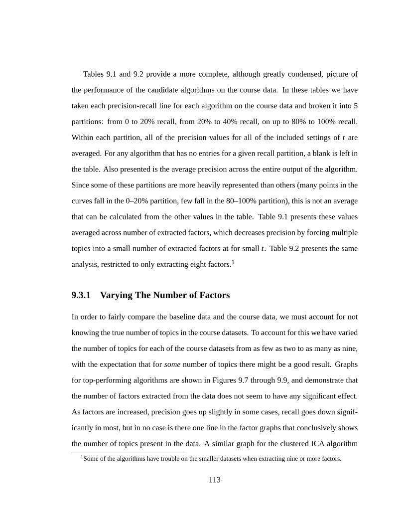
Tables9.1 and9.2 provide a more complete, although greatly condensed, picture of
the performance of the candidate algorithms on the course data. In these tables we have
taken each precision-recall line for each algorithm on the course data and broken it into 5
partitions: from 0 to 20% recall, from 20% to 40% recall, on up to 80% to 100% recall.
Within each partition, all of the precision values for all of the included settings oft are
averaged. For any algorithm that has no entries for a given recall partition, a blank is left in
the table. Also presented is the average precision across the entire output of the algorithm.
Since some of these partitions are more heavily represented than others (many points in the
curves fall in the 0–20% partition, few fall in the 80–100% partition), this is not an average
that can be calculated from the other values in the table. Table9.1 presents these values
averaged across number of extracted factors, which decreases precision by forcing multiple
topics into a small number of extracted factors at for smallt. Table9.2 presents the same
analysis, restricted to only extracting eight factors.1
9.3.1 Varying The Number of Factors
In order to fairly compare the baseline data and the course data, we must account for not
knowing the true number of topics in the course datasets. To account for this we have varied
the number of topics for each of the course datasets from as few as two to as many as nine,
with the expectation that forsomenumber of topics there might be a good result. Graphs
for top-performing algorithms are shown in Figures9.7 through9.9, and demonstrate that
the number of factors extracted from the data does not seem to have any significant effect.
As factors are increased, precision goes up slightly in some cases, recall goes down signif-
icantly in most, but in no case is there one line in the factor graphs that conclusively shows
the number of topics present in the data. A similar graph for the clustered ICA algorithm
1Some of the algorithms have trouble on the smaller datasets when extracting nine or more factors.
113
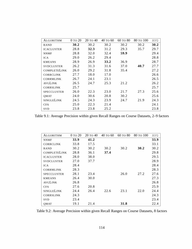
ALGORITHM 0 TO 20 20TO 40 40TO 60 60TO 80 80TO 100 AVGRAND 30.2 30.2 30.2 30.2 30.2 30.2ICACLUSTER 28.8 32.3 31.2 29.3 35.7 29.7NNMF 28.8 32.0 32.4 59.9 29.4ICA 29.0 26.2 29.4 28.8KMEANS 28.9 26.9 33.2 36.9 28.7SVDCLUSTER 26.2 31.3 31.6 37.0 40.7 27.7COMPLETEL INK 26.0 29.2 31.8 35.4 27.2CORRCLINK 27.7 18.0 17.0 26.6CORRMLINK 26.7 24.1 23.1 26.5AVGL INK 26.5 24.7 25.3 21.2 26.2CORRSLINK 25.7 25.7SPECCLUSTER 26.0 22.3 23.0 21.7 27.3 25.6QMAT 24.0 30.6 20.8 30.2 25.6SINGLEL INK 24.5 24.3 23.9 24.7 21.9 24.3CFA 25.0 22.3 21.4 24.1SVD 23.8 23.8 25.2 23.8
Table 9.1: Average Precision within given Recall Ranges on Course Datasets, 2–9 factors
ALGORITHM 0 TO 20 20TO 40 40TO 60 60TO 80 80TO 100 AVGNNMF 33.9 41.2 33.9CORRCLINK 33.8 17.5 33.1RAND 30.2 30.2 30.2 30.2 30.2 30.2COMPLETEL INK 28.8 36.1 37.4 29.8ICACLUSTER 28.0 38.0 29.5SVDCLUSTER 27.0 37.7 28.9ICA 28.4 28.4CORRMLINK 28.3 28.3SPECCLUSTER 28.1 23.4 26.0 27.2 27.6KMEANS 26.4 30.0 27.3AVGL INK 26.8 26.8CFA 27.6 20.8 25.9SINGLEL INK 24.4 26.4 22.6 23.1 22.0 24.4CORRSLINK 24.3 24.3SVD 23.4 23.4QMAT 19.1 21.4 31.8 22.4
Table 9.2: Average Precision within given Recall Ranges on Course Datasets, 8 factors
114
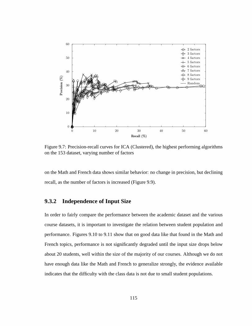
0
10
20
30
40
50
60
Pre
cis
ion
(%)
Pre
cis
ion
(%)
0 10 20 30 40 50 60
Recall (%)Recall (%)
2 factors
3 factors
4 factors
5 factors
6 factors
7 factors
8 factors
9 factors
Random
Figure 9.7: Precision-recall curves for ICA (Clustered), the highest performing algorithmson the 153 dataset, varying number of factors
on the Math and French data shows similar behavior: no change in precision, but declining
recall, as the number of factors is increased (Figure9.9).
9.3.2 Independence of Input Size
In order to fairly compare the performance between the academic dataset and the various
course datasets, it is important to investigate the relation between student population and
performance. Figures9.10to 9.11show that on good data like that found in the Math and
French topics, performance is not significantly degraded until the input size drops below
about 20 students, well within the size of the majority of our courses. Although we do not
have enough data like the Math and French to generalize strongly, the evidence available
indicates that the difficulty with the class data is not due to small student populations.
115
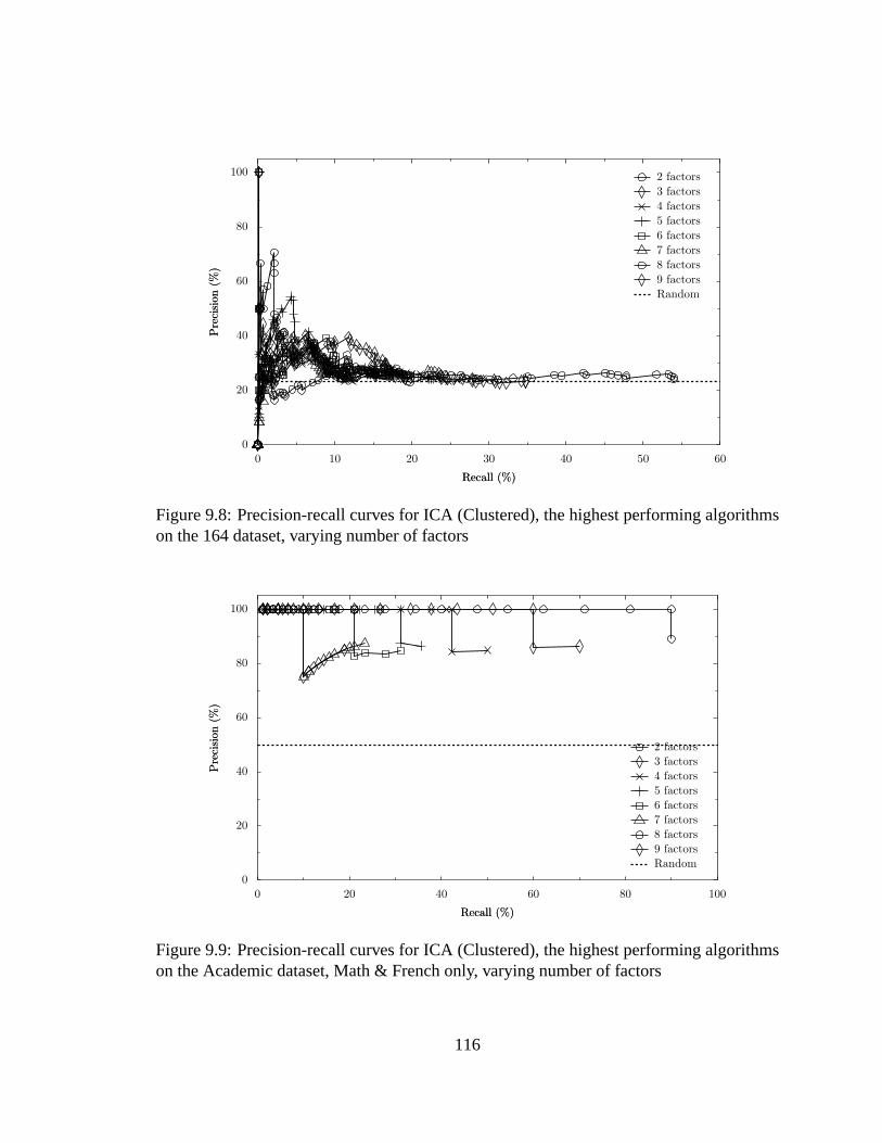
0
20
40
60
80
100
Pre
cis
ion
(%)
Pre
cis
ion
(%)
0 10 20 30 40 50 60
Recall (%)Recall (%)
2 factors
3 factors
4 factors
5 factors
6 factors
7 factors
8 factors
9 factors
Random
Figure 9.8: Precision-recall curves for ICA (Clustered), the highest performing algorithmson the 164 dataset, varying number of factors
0
20
40
60
80
100
Pre
cis
ion
(%)
Pre
cis
ion
(%)
0 20 40 60 80 100
Recall (%)Recall (%)
2 factors
3 factors
4 factors
5 factors
6 factors
7 factors
8 factors
9 factors
Random
Figure 9.9: Precision-recall curves for ICA (Clustered), the highest performing algorithmson the Academic dataset, Math & French only, varying number of factors
116

0
20
40
60
80
100
Pre
cis
ion
(%)
Pre
cis
ion
(%)
0 20 40 60 80
Recall (%)Recall (%)
Full Data
25% (m=67)
10% (m=27)
5% (m=13)
Random
Figure 9.10: Varying population size on Academic dataset, ICA (Clustered), 4 factors
0
20
40
60
80
100
Pre
cis
ion
(%)
Pre
cis
ion
(%)
0 20 40 60 80 100
Recall (%)Recall (%)
Full Data
25% (m=67)
10% (m=27)
5% (m=13)
Random
Figure 9.11: Varying population size on Academic dataset, Math & French only, 2 factors
117

9.3.3 Free-Response vs. Multiple-Choice
Given that our 141 dataset is the only course dataset that is a good candidate for containing
topic information, and that the 141 dataset is the only one generated purely from free-
response questions, it is worth investigating the hypothesis that multiple-choice questions
confound topic extraction. This is also supported by the academic and trivial quiz baseline
quizzes, which were presented as short answer free-response questions.
Of the five available datasets, three are homogeneous question types: the 008 and 010
datasets are all multiple choice, the 141 is all free-response. The 153 dataset is mixed, but
contains only seven free-response questions. Looking at the human-generated groupings
that are made up of only free-response questions, there are only four pairs of questions that
are labelled “acceptable.” This is too small to provide significant results. The fifth course
dataset (164) is mixed, and contains 42 free-response questions and 30 multiple-choice.
Regrettably, this is the only dataset available for us to evaluate the this hypothesis.
When the free-response and multiple-choice questions are separated from each other in
the 164 dataset, we see again that the algorithms that perform well are those that assume
linear relationships among the topic factors, but no algorithm stands out as being the correct
answer. From a comparison of the free-response plot (Figure9.12) and the multiple-choice
plot (Figure9.13), there is little difference, but any advantage would seem to favor the mul-
tiple choice questions. Question type does not appear to be a strong role in the separability
of a score matrix.
9.3.4 Q-Matrix Model Mismatch
Of the entire candidate set, the slowest algorithm is our implementation of Q-Matrix. This
may partially be because of inexperience with it, or poor performance choices. However, a
118

0
20
40
60
80
100
Pre
cis
ion
(%)
Pre
cis
ion
(%)
0 5 10 15 20 25 30 35
Recall (%)Recall (%)
ICA (Clustered)
Correlated Complete-Linkage
NNMF
Correlated Mean-Linkage
SVD (Clustered)
Random
Figure 9.12: Best five algorithms, 164 dataset, free-response only
0
20
40
60
80
100
Pre
cis
ion
(%)
Pre
cis
ion
(%)
0 10 20 30 40 50
Recall (%)Recall (%)
Correlated Single-Linkage
SVD (Clustered)
Correlated Complete-Linkage
ICA
Correlated Mean-Linkage
Random
Figure 9.13: Best five algorithms, 164 dataset, multiple-choice only
119
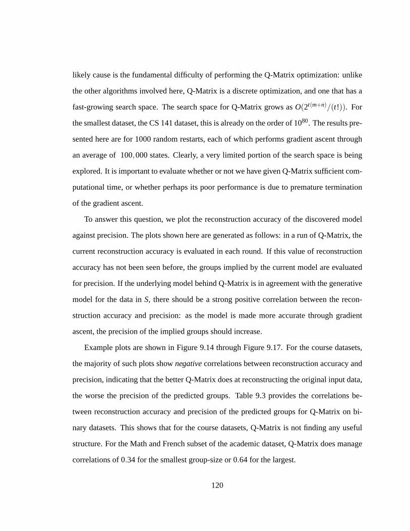
likely cause is the fundamental difficulty of performing the Q-Matrix optimization: unlike
the other algorithms involved here, Q-Matrix is a discrete optimization, and one that has a
fast-growing search space. The search space for Q-Matrix grows asO(2t(m+n)/(t!)). For
the smallest dataset, the CS 141 dataset, this is already on the order of 1080. The results pre-
sented here are for 1000 random restarts, each of which performs gradient ascent through
an average of 100,000 states. Clearly, a very limited portion of the search space is being
explored. It is important to evaluate whether or not we have given Q-Matrix sufficient com-
putational time, or whether perhaps its poor performance is due to premature termination
of the gradient ascent.
To answer this question, we plot the reconstruction accuracy of the discovered model
against precision. The plots shown here are generated as follows: in a run of Q-Matrix, the
current reconstruction accuracy is evaluated in each round. If this value of reconstruction
accuracy has not been seen before, the groups implied by the current model are evaluated
for precision. If the underlying model behind Q-Matrix is in agreement with the generative
model for the data inS, there should be a strong positive correlation between the recon-
struction accuracy and precision: as the model is made more accurate through gradient
ascent, the precision of the implied groups should increase.
Example plots are shown in Figure9.14through Figure9.17. For the course datasets,
the majority of such plots shownegativecorrelations between reconstruction accuracy and
precision, indicating that the better Q-Matrix does at reconstructing the original input data,
the worse the precision of the predicted groups. Table9.3 provides the correlations be-
tween reconstruction accuracy and precision of the predicted groups for Q-Matrix on bi-
nary datasets. This shows that for the course datasets, Q-Matrix is not finding any useful
structure. For the Math and French subset of the academic dataset, Q-Matrix does manage
correlations of 0.34 for the smallest group-size or 0.64 for the largest.
120

0
20
40
60
80
100
Pre
cis
ion
(%)
Pre
cis
ion
(%)
30 40 50 60 70
Reconstruction Accuracy (%)Reconstruction Accuracy (%)
Figure 9.14: Q-Matrix Reconstruction vs. Precision for 010 dataset, 9 factors. Minimalgroup size.
7.5
10
12.5
15
17.5
20
22.5
Pre
cis
ion
(%)
Pre
cis
ion
(%)
30 40 50 60 70
Reconstruction Accuracy (%)Reconstruction Accuracy (%)
Figure 9.15: Q-Matrix Reconstruction vs. Precision for 010 dataset, 9 factors. Maximalgroup size.
121
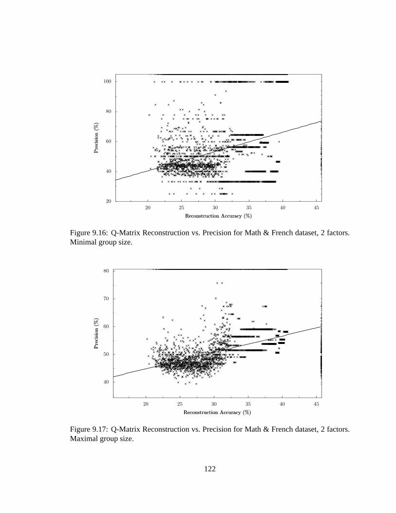
20
40
60
80
100
Pre
cis
ion
(%)
Pre
cis
ion
(%)
20 25 30 35 40 45
Reconstruction Accuracy (%)Reconstruction Accuracy (%)
Figure 9.16: Q-Matrix Reconstruction vs. Precision for Math & French dataset, 2 factors.Minimal group size.
40
50
60
70
80
Pre
cis
ion
(%)
Pre
cis
ion
(%)
20 25 30 35 40 45
Reconstruction Accuracy (%)Reconstruction Accuracy (%)
Figure 9.17: Q-Matrix Reconstruction vs. Precision for Math & French dataset, 2 factors.Maximal group size.
122

MATH & FRENCH TRIVIA 008 010HIGH INCLUSIVENESS 0.64 0.1 -0.85 -0.14LOW INCLUSIVENESS 0.34 -0.08 -0.03 -0.05
Table 9.3: Correlation of reconstruction accuracy vs. precision on binary datasets
9.3.5 Removing Low-Discrimination Questions
If we assume that much of the difficulty in grouping questions by topic is the fact that stu-
dent scores are noisy, then an obvious line of investigation is to try to remove questions that
are particularly noisy before performing our clustering. Utilizing the technique introduced
in Chapter7, we can discard questions that have a discriminationα below some threshold.
While this will reduce the number of questions that get clustered, it does have the benefit
of only clustering the questions that we believe are most meaningful. Dropping questions
with α ≤ 0.75, the “bad” questions, reduces the number of questions in the course datasets
by an average of 42.5%. Running the full suite of algorithms against these reduced datasets
produces the summaries given in Table9.4and Table9.5.
The results here indicate that dropping the low-discrimination questions does indeed
lead to slightly better results. When compared to Table9.1, Table9.4 has a few notable
features. Most importantly, even when averaged over the whole factor range, the high
discrimination questions yield three algorithms that are able to beat random chance on this
data. Here SVD,k-means, and ICA are all slightly above random chance, although even
the best is within 1% of the random chance performance.
A better measure of the precision overall is again to look at the single large-factor
table, Table9.5. By overestimating the number of topics we eliminate the possibility of
an algorithm producing correct clusters and being forced by the pigeonhole principle to
group two unrelated clusters together. Table9.5 provides the precision values fort = 8
123

ALGORITHM 0 TO 20 20TO 40 40TO 60 60TO 80 80TO 100 AVGSVD 33.7 37.7 33.7KMEANS 33.0 35.6 36.9 33.4ICA 33.3 40.7 33.3RAND 32.8 32.8 32.8ICACLUSTER 32.5 35.9 36.8 32.8SVDCLUSTER 31.9 36.3 36.3 32.3SPECCLUSTER 31.2 23.4 36.2 32.1NNMF 31.0 36.9 31.1CORRSLINK 31.0 31.0CORRMLINK 29.5 31.7 29.5CORRCLINK 28.6 42.1 28.9CFA 28.0 35.4 28.1SINGLEL INK 27.7 26.8 36.4 27.9AVGL INK 25.4 31.2 25.5COMPLETEL INK 23.4 31.7 35.9 24.5QMAT 16.6 20.2 16.8
Table 9.4: Average Precision within given Recall Ranges on Course Datasets, 2–9 factors,only questions withα > 0.75
on the high-discrimination data. Here we expect the average recall values to be lower,
but precision to be higher as there is less forcing of unrelated topics into the same factor.
On this table, the best-performing algorithm is the single-linkage agglomerative clustering
applied to the correlation matrix, with a 41.1% average recall, which is notably higher than
the random probability of 33.4%.
Precision vs. Discrimination
The effectiveness of this technique is definitely a function of the cutoff point forα that is
used: at lowα, where few are removed, we get performance as shown in Table9.1: random
chance outperforms anything we have investigated. On the opposite extreme, where many
questions are dropped, we have likely lost all of the topic information, as the questions that
are kept are going to be the questions that have the most in common with the whole set of
124
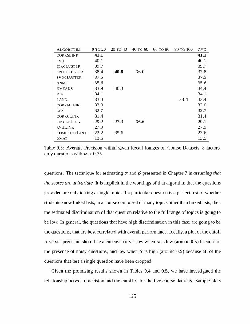
ALGORITHM 0 TO 20 20TO 40 40TO 60 60TO 80 80TO 100 AVGCORRSLINK 41.1 41.1SVD 40.1 40.1ICACLUSTER 39.7 39.7SPECCLUSTER 38.4 40.8 36.0 37.8SVDCLUSTER 37.5 37.5NNMF 35.6 35.6KMEANS 33.9 40.3 34.4ICA 34.1 34.1RAND 33.4 33.4 33.4CORRMLINK 33.0 33.0CFA 32.7 32.7CORRCLINK 31.4 31.4SINGLEL INK 29.2 27.3 36.6 29.1AVGL INK 27.9 27.9COMPLETEL INK 22.2 35.6 23.6QMAT 13.5 13.5
Table 9.5: Average Precision within given Recall Ranges on Course Datasets, 8 factors,only questions withα > 0.75
questions. The technique for estimatingα andβ presented in Chapter7 is assuming that
the scores are univariate.It is implicit in the workings of that algorithm that the questions
provided are only testing a single topic. If a particular question is a perfect test of whether
students know linked lists, in a course composed of many topics other than linked lists, then
the estimated discrimination of that question relative to the full range of topics is going to
be low. In general, the questions that have high discrimination in this case are going to be
the questions, that are best correlated with overall performance. Ideally, a plot of the cutoff
α versus precision should be a concave curve, low whenα is low (around 0.5) because of
the presence of noisy questions, and low whenα is high (around 0.9) because all of the
questions that test a single question have been dropped.
Given the promising results shown in Tables9.4 and 9.5, we have investigated the
relationship between precision and the cutoffα for the five course datasets. Sample plots
125
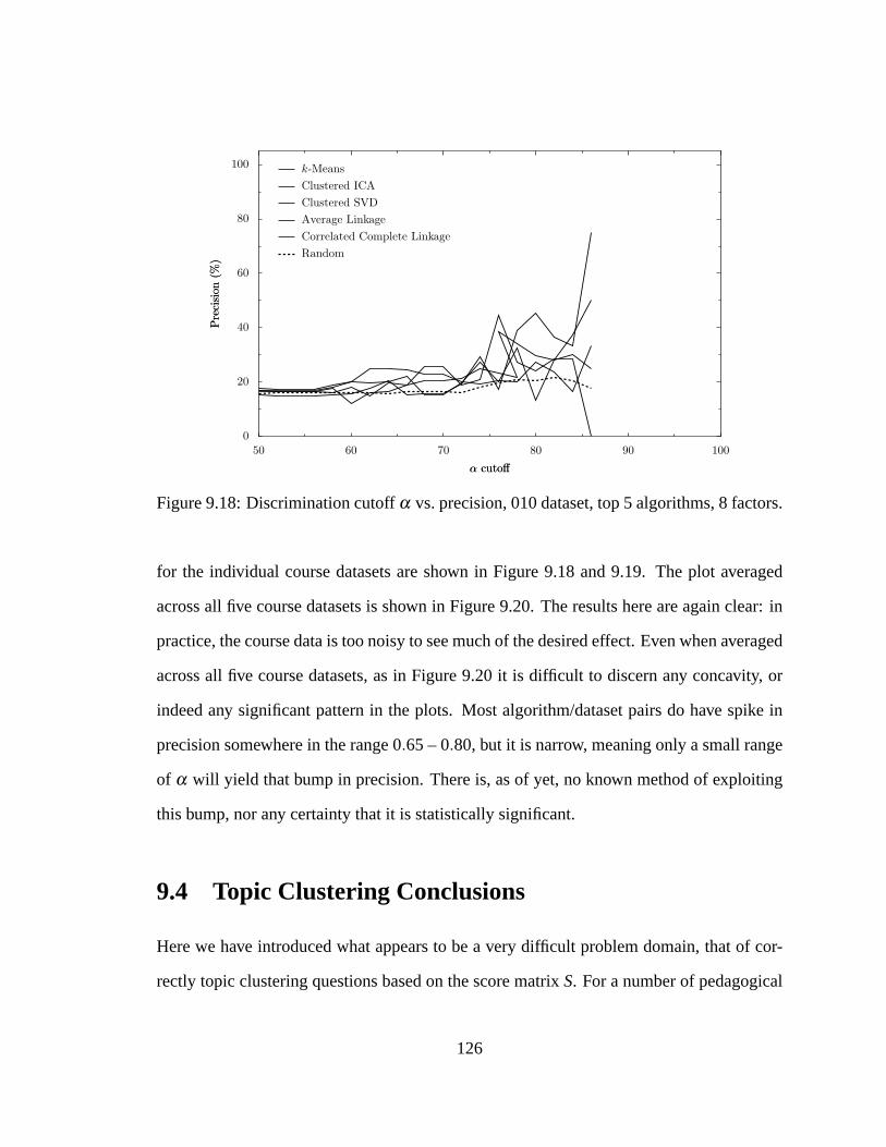
0
20
40
60
80
100
Pre
cis
ion
(%)
Pre
cis
ion
(%)
50 60 70 80 90 100
α cutoffα cutoff
k-Means
Clustered ICA
Clustered SVD
Average Linkage
Correlated Complete Linkage
Random
Figure 9.18: Discrimination cutoffα vs. precision, 010 dataset, top 5 algorithms, 8 factors.
for the individual course datasets are shown in Figure9.18and9.19. The plot averaged
across all five course datasets is shown in Figure9.20. The results here are again clear: in
practice, the course data is too noisy to see much of the desired effect. Even when averaged
across all five course datasets, as in Figure9.20it is difficult to discern any concavity, or
indeed any significant pattern in the plots. Most algorithm/dataset pairs do have spike in
precision somewhere in the range 0.65 – 0.80, but it is narrow, meaning only a small range
of α will yield that bump in precision. There is, as of yet, no known method of exploiting
this bump, nor any certainty that it is statistically significant.
9.4 Topic Clustering Conclusions
Here we have introduced what appears to be a very difficult problem domain, that of cor-
rectly topic clustering questions based on the score matrixS. For a number of pedagogical
126
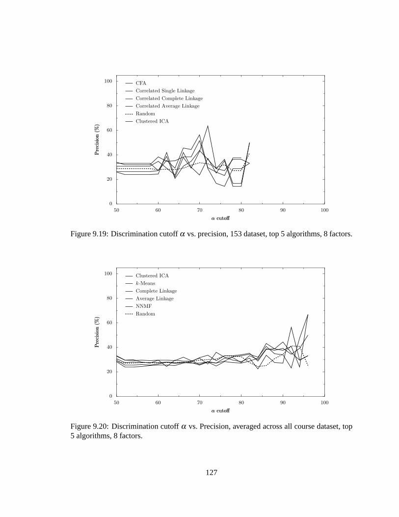
0
20
40
60
80
100
Pre
cis
ion
(%)
Pre
cis
ion
(%)
50 60 70 80 90 100
α cutoffα cutoff
CFA
Correlated Single Linkage
Correlated Complete Linkage
Correlated Average Linkage
Random
Clustered ICA
Figure 9.19: Discrimination cutoffα vs. precision, 153 dataset, top 5 algorithms, 8 factors.
0
20
40
60
80
100
Pre
cis
ion
(%)
Pre
cis
ion
(%)
50 60 70 80 90 100
α cutoffα cutoff
Clustered ICA
k-Means
Complete Linkage
Average Linkage
NNMF
Random
Figure 9.20: Discrimination cutoffα vs. Precision, averaged across all course dataset, top5 algorithms, 8 factors.
127

and assessment reasons, this is an important problem. However, at this point it appears
that none of the algorithms in this survey have any reliable success on this problem for
the targeted datasets. On score data generated by extremely different topics testing deeply
learned skills, choice of algorithm makes relatively little difference. The majority of sim-
ple algorithms work well on such data. However, on score data from actual courses, all
surveyed algorithms perform similarly to random chance, with very few outperforming
chance. Those that do outperform generally imply a linear model with high noise underly-
ing the data.
Whether this is a failure of modern machine learning methods, of the experimenters for
not finding the right algorithms in this survey, or of the teachers of the various courses, can-
not be answered at this time. Regardless of the source of the problem, the results presented
here highlight the complexities found in score-based educational data mining: relatively
small datasets, high levels of noise, and unknown generative processes.
128

Chapter 10
Clustering with Partial Topic
Information
Although nothing presented in Chapter9 works well enough to be considered a solution
to the topic clustering problem, any automation in the generation ofR is beneficial for
our assessment project. We have therefore investigated semi-supervised clustering of the
questions represented inS. Some algorithms, like SVD or ICA, cannot be easily adapted
into a semi-supervised form. Others, like NNMF, Q-Matrix, or any of the agglomerative
clustering algorithms, can be adapted quite easily. The primary concern in this section is to
determine the usefulness of providing partial information. If it is the case that identifying
a single group membership for 25% of the questions is sufficient to provide high-precision
results, then we can easily justify asking instructors for partial information and algorithmi-
cally determine the remainder1. If it requires 75% of the questions to be identified, then
it is likely to be more efficient to simply ask the instructors for a full labelling, without
resorting to algorithmic methods.
1It is also worth noting that in doing so, it may belesswork for instructors, as the labels on the clusterscan be carried over from the partial information, preventing any post-clustering prompt of the instructor.
129

10.1 Hints Provided
In order to continue this analysis with the datasets used in previous chapters, it is necessary
for us to develop a method of providing partial information for the algorithms based on the
human groupings, rather than the relevance matrixR directly. SinceR could be generated
from the human groupings, this means that the partial information is provided in terms of
sets of questions that should be clustered, rather than subset of entries fromR.
The hint that is provided to each algorithm is determined as follows. Hints are deter-
mined based on a hint percentagep and number of topicst, as follows.
• The hint is initialized as a full copy of the correct answer.
• For each question in the dataset, we include information about it in the hint with
probability p.
• If a question is not selected, then that all information about that question is removed
from the hint.
• The final hint is composed of thek largest sets. We iteratively select each of these
sets.
• When a set is selected as part of the final hint, each question in that set is removed
from any other hint sets. This ensures each question is only in a single set, to be
comparable with the topic clustering experiment of Chapter92.
2All algorithms from Chapter9 except Q-Matrix placed questions in exactly one group
130

10.2 Algorithms
In this investigation we are looking at a subset of the algorithms utilized in Chapter9.
Specifically we are looking at the following algorithms:
10.2.1 k-means
Thek-means clustering algorithm can be extended to utilize partial relevance by providing
it a listing of questions that must be placed together. Given the set of correctly-grouped
questions, we can move each known question to the mean of the group it appears in. Thus
if three questions are known to be grouped together, we replace the original coordinates for
each of them with a new vector at their mean. Correct weighting of the importance of that
point is ensured by retaining three copies of it in the dataset.
This is equivalent to leaving the points in place and altering the code to ensure that
those points are always grouped together. By moving the points to be co-located, we are
guaranteed they will be placed into the same group. By choosing that point to be at their
mean, we ensure that they have the same effect on their assigned cluster center that the
three of them together would have. Performing the alteration this way allows the partial-
information result to be done as a pre-processing step, without altering the code itself.
10.2.2 Agglomerative Clustering
Both the raw (Euclidean) and correlated agglomerative clustering algorithms can easily
be extended with partial information by simply changing the starting condition from hav-
ing every question independently grouped, to initializing groups of questions that must be
paired together. The algorithms proceed as normal after initialization.
131

10.2.3 NNMF
During each round of the gradient ascent for the NNMF algorithm, we can overwrite entries
in the relevance vectors for those questions that need to be placed together. As in thek-
means case, this is done by finding the factor to which the set of questions can most easily
be assigned to. For each question whose assignment is “known,” we ensure at each step
that the entry corresponding to the correct group is set to 1 and the other entries for that
question are set to 0.
10.2.4 Q-Matrix
Modification of Q-Matrix is easy, as the output from Q-Matrix most closely represents what
we are looking for: a binary assignment of questions into topic groups. Here the Q-Matrix
is initialized such that the desired group memberships are guaranteed. As in the NNMF
case, the entry for the correct group for each known question is set to 1 and all other entries
are set to 0. Questions that are known are not updated during the gradient ascent.
10.3 Results
When evaluating results for this experiment, we are focused primarily on the final precision
values. Since the algorithms tested are assigning each question to exactly one group, and
some of the questions are assigned to more than one group in the human-generated answer,
recall values have less absolute meaning. However, every algorithm should be able to
produce 100% accuracy when presented with 100% of the correct answer. The hope is to
discover one or more algorithms that can produce perfect or near-perfect accuracy with a
small amount of the answer provided.
132
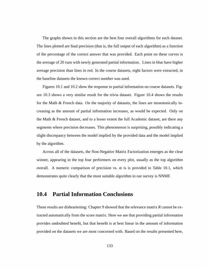
The graphs shown in this section are the best four overall algorithms for each dataset.
The lines plotted are final precision (that is, the full output of each algorithm) as a function
of the percentage of the correct answer that was provided. Each point on these curves is
the average of 20 runs with newly generated partial information. Lines in blue have higher
average precision than lines in red. In the course datasets, eight factors were extracted, in
the baseline datasets the known correct number was used.
Figures10.1and10.2show the response to partial information on course datasets. Fig-
ure 10.3shows a very similar result for the trivia dataset. Figure10.4 shows the results
for the Math & French data. On the majority of datasets, the lines are monotonically in-
creasing as the amount of partial information increases, as would be expected. Only on
the Math & French dataset, and to a lesser extent the full Academic dataset, are there any
segments where precision decreases. This phenomenon is surprising, possibly indicating a
slight discrepancy between the model implied by the provided data and the model implied
by the algorithm.
Across all of the datasets, the Non-Negative Matrix Factorization emerges as the clear
winner, appearing in the top four performers on every plot, usually as the top algorithm
overall. A numeric comparison of precision vs.α is is provided in Table10.1, which
demonstrates quite clearly that the most suitable algorithm in our survey is NNMF.
10.4 Partial Information Conclusions
These results are disheartening: Chapter9 showed that the relevance matrixRcannot be ex-
tracted automatically from the score matrix. Here we see that providing partial information
provides undoubted benefit, but that benefit is at best linear in the amount of information
provided on the datasets we are most concerned with. Based on the results presented here,
133

0
20
40
60
80
100
Fin
al
Pre
cis
ion
(%)
Fin
al
Pre
cis
ion
(%)
0 20 40 60 80 100
Hint Size (%)Hint Size (%)
NNMF
Average Linkage
k-Means
Complete Linkage
Random
Figure 10.1: Best four algorithms, 008 dataset
0
20
40
60
80
100
Fin
al
Pre
cis
ion
(%)
Fin
al
Pre
cis
ion
(%)
0 20 40 60 80 100
Hint Size (%)Hint Size (%)
Correlated Single Linkage
Correlated Complete Linkage
Correlated Average Linkage
NNMF
Random
Figure 10.2: Best four algorithms, 141 dataset
134
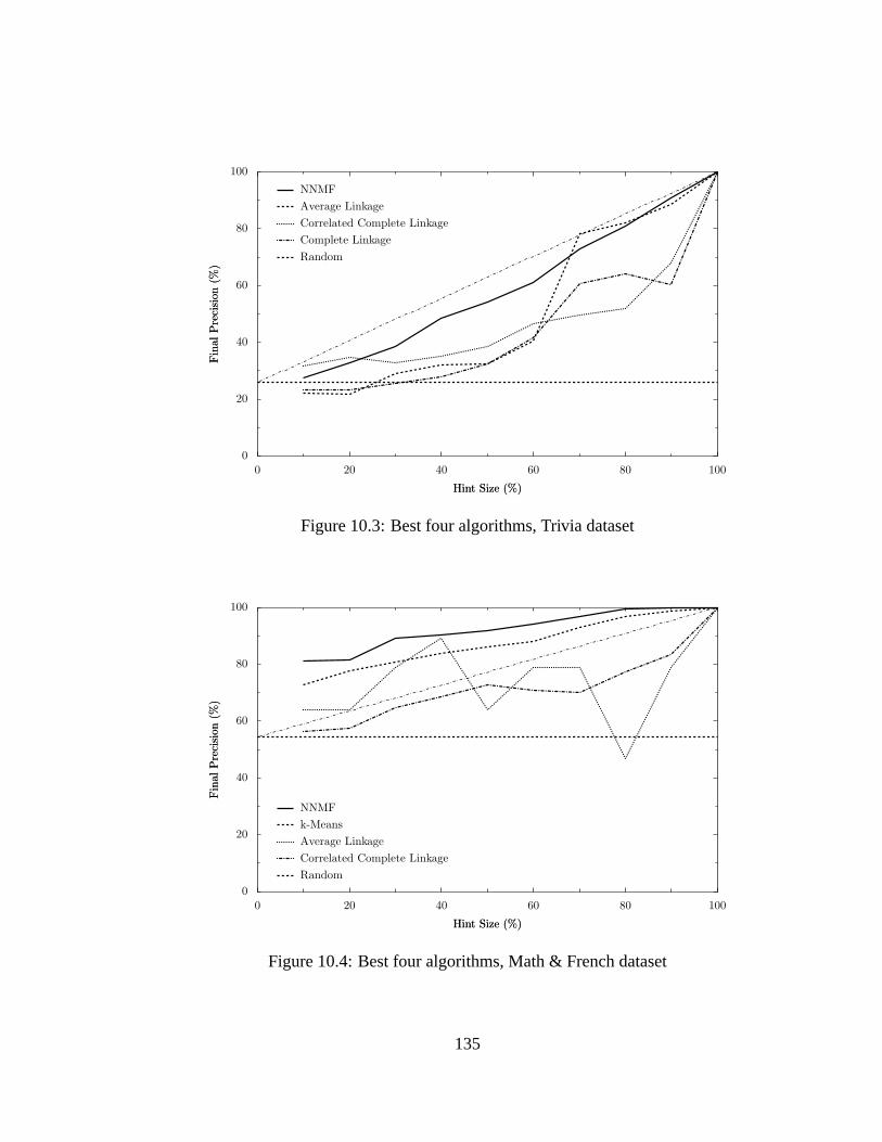
0
20
40
60
80
100
Fin
al
Pre
cis
ion
(%)
Fin
al
Pre
cis
ion
(%)
0 20 40 60 80 100
Hint Size (%)Hint Size (%)
NNMF
Average Linkage
Correlated Complete Linkage
Complete Linkage
Random
Figure 10.3: Best four algorithms, Trivia dataset
0
20
40
60
80
100
Fin
al
Pre
cis
ion
(%)
Fin
al
Pre
cis
ion
(%)
0 20 40 60 80 100
Hint Size (%)Hint Size (%)
NNMF
k-Means
Average Linkage
Correlated Complete Linkage
Random
Figure 10.4: Best four algorithms, Math & French dataset
135
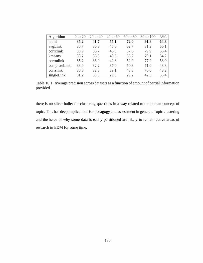
Algorithm 0 to 20 20 to 40 40 to 60 60 to 80 80 to 100AVGnnmf 35.2 41.7 55.1 72.0 91.8 64.8avgLink 30.7 36.3 45.6 62.7 81.2 56.1corrclink 33.9 36.7 46.0 57.6 79.9 55.4kmeans 33.7 36.5 43.5 55.2 79.1 54.2corrmlink 35.2 36.0 42.8 52.9 77.2 53.0completeLink 33.0 32.2 37.0 50.3 71.0 48.3corrslink 30.8 32.8 39.1 48.8 70.0 48.2singleLink 31.2 30.0 29.0 29.2 42.5 33.4
Table 10.1: Average precision across datasets as a function of amount of partial informationprovided.
there is no silver bullet for clustering questions in a way related to the human concept of
topic. This has deep implications for pedagogy and assessment in general. Topic clustering
and the issue of why some data is easily partitioned are likely to remain active areas of
research in EDM for some time.
136

Chapter 11
Future of EDM
The field of Educational Data Mining is ripe for explosive growth. Machine learning and
data mining have developed a vast array of tools and techniques that have been well-studied
and examined in myriad contexts. However, as seen in earlier chapters, EDM is still an
extremely small field, with an estimated thirty researchers worldwide identifying as being
interested in it. Given the strong ITS background for many EDM researchers, it is certain
that the ITS community will have a strong presence in EDM in years to come, but the focus
is likely to shift from being a sub-division of the ITS community into a broader discipline
operating in the overlap between education, pedagogy, machine learning, and statistics. In
this chapter we will discuss some avenues for future work based on the research presented
in this dissertation, as well as general predictions of where EDM as a whole will go during
the next few years.
137

11.1 Future Work
As with any other significant research project, it is difficult or impossible to find a point at
which the research presented in this dissertation is “done.” In this case, there are a number
of avenues for future work that have already presented themselves. It is unlikely that I will
be able to follow up on every one of these research paths, but I hope to investigate the
majority of the following.
11.1.1 Other “Baseline” Topics
In the academic baseline dataset presented in the topic clustering experiment, why is it that
Math and French are separable, but Biology and World History are not? What other sub-
jects are separable? It seems obvious that languages ought to be separable from sciences,
given that Math is separable from French. Are languages separable from one another?
Is Italian separable from French? Is Japanese separable from Spanish? Within the more
technical areas, are highly-mathematical subjects like Physics separable from Math? Per-
forming follow-up data collection and experimentation with the topic clustering framework
developed for this dissertation should provide some insight into what subjects are funda-
mentally separable. Of particular interest to the CS Education research community would
be whether an online quiz of this type that focused purely on computer science topics are
separable. The results of that would indicate whether or not it is the type of assessment we
perform in class, in relation towhenwe perform that assessment relative to the initial intro-
duction of the knowledge, that is truly important. There is a significant amount of research
that could be performed in this vein, with applicability to cognition, education, assessment,
and education, in addition to EDM.
138
11.1.2 Distinct Sizes of Cognitively Related Information
Another interpretation of the results of the topic clustering analysis experiment is that there
is a fundamentally different behavior for questions that are related at the “topic” level than
those that are related at the subject level. Obviously, a test that was checking for the pres-
ence or absence of individual pieces of isolated knowledge can determine whether a student
has learned those pieces of knowledge. The results from the topic clustering experiment
suggest that we can determine who has studied Math or French (and still remembers it), but
for some reason cannot determine who understands linked lists but not hash tables.
It is possible that there is some emergent reason for this discrepancy that could be
modelled using a cognitive architecture like ACT-R or SOAR. This style of cognitive ex-
periment is not unheard of in the cognition community, as shown by research like (Peterson
and Simon, 2000).
11.1.3 Voting Methods for Topic Clustering
Since the algorithms presented in the experiment on topic clustering with partial informa-
tion all perform better than random chance given 25% to 30% of the answer, there is a
possibility of leveraging this into creating a more precise aggregate answer. Voting meth-
ods are based on the idea of giving votes to a number of classifiers, each of which is better
than random. Not all voters have equal sway in the final results, but the answer with the
most votes is the final prediction. In this case algorithms would be voting for individual
question pairings, and it is possible that from those pairings an aggregate answer could be
produced. One requirement for this to work would be that the algorithms produce distinct
pairings, rather than all producing the same (relatively inaccurate) answer. Preliminary in-
vestigations into this indicate that the overlap between pairings produced by the algorithms
139
in the topic clustering experiment are relatively slight, so this should not be much of a con-
cern. This recalls some of the work done recently on mixing clustering algorithms (Gionis
et al., 2005).
11.1.4 Alternate UI Platforms for Agar
Although rather more mundane that some of the other research, the focus on usability
that went into the development of Agar makes it a prime candidate for experimentation
into other UI platforms. Two user interface platforms in particular are of great interest:
development of an Agar variant for use with Tablet PC technology, which enables the “red-
pen” metaphor to an even greater extent, and an online version of Agar using the currently
popular AJAX (asynchronous Javascript and XML) suite of technologies, allowing for easy
onetime backend setup and ubiquitous access to CAA systems from any network-enabled
host. While certainly less research-oriented than other avenues of future work, development
of systems like these would undoubtedly be a benefit for the academic community at large.
11.2 The Road Ahead
The current dominance of ITS-related research and datasets is clear in the EDM commu-
nity. Of the two past EDM workshops, one was at the International Conference on Intelli-
gent Tutoring Systems, and the other was at the AAAI yearly conference. As of this writing
there are calls for papers for two new EDM workshops in 2006. Again, one is located at
ICITS and the other is at AAAI.
However, this dominance is dimming somewhat as the community grows and diversi-
fies. More EDM research is being presented from non-ITS data sources, ranging from the
unit-test score matrices (Spacco et al., 2006) of the Marmoset project (Spacco et al., 2005)
140

to standardized test data. Indeed, the full cross-product of educational data sources and
machine learning techniques provides a fertile ground for future EDM research.
Perhaps the single most intriguing data source that has yet to be taken advantage of is
the collection of novice programmer code snapshots stored by the Marmoset project. These
snapshots are taken during the development of the students’ first programming projects,
stored every time each student saves their code. There are literally hundreds of thousands
of these snapshots available. Obviously, dealing with such a rich data source will require
some advanced techniques, as hand-coding for descriptive features of each snapshot is quite
infeasible. However, such a large and rich source of data is quite tantalizing: behavior
of first-year programming students has been a continual theme of investigation in the CS
Education community for decades (Gruener and Graziano, 1978; McCracken et al., 2001).
Given the resources to investigate the behavioral patterns shown in such data, the Marmoset
data could easily become a seminal hallmark of the EDM community.
If data mining is really “statistics on steroids,” by analogy, educational data mining
must be educational statistics on steroids. If there is any truth in this analogy, then an obvi-
ous and critical step in the development of EDM is to look at the techniques that have come
out of educational statistics or psychometrics to see where EDM techniques can be applied.
A prime example of this is the research presented on estimating difficulty and discrimina-
tion statistics for student population sizes too small to utilize IRT (Chapter7). Statistical
techniques that need to be examined by the EDM community include CFA, Cronbach’s
Alpha (Cronbach, 1951), validity, and reliability.
One of the major outstanding questions in the future of EDM is with which fields it will
develop significant ties. While it is almost certain that EDM will retain ties with the ITS
community for quite some time, the possibility of overlap with other areas will bring EDM
into the awareness of a broader audience. The growth of EDM will obviously be affected
141

by the areas that EDM becomes connected with. EDM could easily see growth in the field
of machine learning, CS Education Research (which is itself somewhat distinct from CS
Education in general), AI in Education, or even general AI, as the issues of prediction, cog-
nition, and learning that surround EDM are central components of much of AI. The fields
that EDM overlaps with will depend very heavily on the EDM-related conferences and
workshops that EDM researchers try to publish in over the next few years. The acceptance
or rejection of all of these fields individually bring independent benefits and drawbacks for
the development of the field as a whole. Stronger connections with machine learning and
AI will bring better experimental procedure to the field, but will pull it further away from
the majority of the instructors that could benefit from ideas coming out of EDM. Inclusion
in the CS education or CS education research communities will bring greater attention to a
broad audience of people interested in improving teaching, assessment, and pedagogy, but
these fields carry with them some stigma of being lower quality research when compared
to more traditional Computer Science.
Perhaps the single most important field for cross-pollination with EDM is that of ed-
ucational statistics and psychometrics. Given the relative dissimilarity of techniques and
experimental methods, this may also be the hardest area for EDM to break into. However,
EDM cannot really be considered a success in its ostensible mission to find non-obvious
information in educational data until the educational statisticians become comfortable with
the results being produced within the EDM community. Without being able to provide the
next generation of tools for organizations like the Educational Testing Service (ETS) and
The College Board to generate and analyze test questions, EDM can only be considered a
partial success at best.
142
Chapter 12
Conclusions
This dissertation describes a method for performing data-driven course assessment and
program assessment as a motivation for a series of investigations into Educational Data
Mining. This type of assessment, both at the course and program levels, is a popular issue
in education today, with renewed emphasis being placed on assessment by accreditation
agencies, parents, administrators, and governments. EDM is uniquely positioned to provide
solutions for difficult assessment problems, such as quantifying student learning, or the
effectiveness of different teaching methods, while still causing only minimal impact on
individual instructors. In situations where standardized testing is too difficult or invasive,
EDM may provide the key to better quantitative assessment.
The bulk of this dissertation focuses on tools and techniques for collection and analysis
of score matrices. Although the analysis fails to provide a solution for low-impact genera-
tion of the relevance matrixR, our collection techniques have proven quite successful, and
automatic generation ofR is merely desirable, not critical, for our program assessment.
143
12.1 Collection
Since most instructors do not currently record scores at the per-item level, it is necessary
to provide methods for gatheringS that make this palatable. In Chapter4 we introduced
two programs that were developed for this task. The first is Agar, a Computer-Aided As-
sessment (CAA) system designed with usability in mind by focusing on existing usage
patterns. The philosophy behind Agar is unique among CAA systems in that Agar works
to fit in with the usage paradigms of instructors, rather than forcing instructors to work
within the restricted usage of the CAA system.
Agar has been deployed and actively used within our department for nearly three years.
The majority of the current users of the system use it voluntarily, and have no connection to
the development of the project. Users are responsible for a slow but steady stream of minor
feature requests, allowing Agar to function more easily in situations that its original design
was never intended to cover. For an academic tool, Agar has seen remarkable success,
growing into a critical component of the departmental teaching infrastructure, rather than
falling by the wayside.
In Chapter4 we also introduced HOMR, the Homebrew Optical Mark Recognition sys-
tem. HOMR allows forms for fill-in-the-bubble surveys, quizzes, and tests to be developed
using a variety of word-processing systems ranging from LATEX to Microsoft Word, printed
on any printer, distributed to students, and scanned on any scanner. With accuracy rates
significantly higher than those utilized by the US Census (Bureau, 2004), HOMR provides
powerful OMR using commodity hardware and an easy programming interface. Such a
tool is ideal for recording scores, either directly by grading multiple-choice tests or by
providing OMR forms for graders to record scores.
144
12.2 Analysis
With tools like Agar and HOMR available to help collect score matrices, it falls to EDM
analysis techniques to determine what assessment information can be extracted fromS. The
analysis techniques presented in this dissertation show a clear progression of what assess-
ment information can be extracted from these score matrices. In Chapter7 we introduced a
method for assessing the difficulty and discrimination of the individual questions, assuming
that the contents of the entire course were related. This is an obvious simplification, but
provides an ability to determine, at minimum, which questions were particularly bad and
possibly which questions were particularly good. By providing estimates of the difficulty
of the question, instructors can ensure that students are understanding concepts at a reason-
able level. By investigating which questions had the worst discrimination, instructors can
begin to train themselves to ask better, more insightful questions, which leads directly to
more meaningful assessment of students.
In Chapter8 we investigated methods for predicting missing entries in the student score
matrix. Based on this investigation, we can see that the statistics gathered in Chapter7 are
useful in predicting scores, particularly on binary score matrices. We also gained some
insight into the structure of score matrices in general, showing that for most prediction
methods it is better to examine other scores on a given question, rather than other scores
by a given student. This reinforces the notion that student scores are noisy, and gives some
justification for the claim made by techniques like CFA that question difficulty is more
important in prediction than student ability, or at least student scores on other questions.
Chapter9 delves into one of the fundamental issues in this assessment system: whether
we can group questions by topic, allowing instructors to generate a binary version of the
relevance matrixR by identifying the topics fort groups of questions, rather than identify-
145
ing the topics for every individual question. Although manually labelling the questions is
possible, likely taking half an hour to an hour per course, it would be preferable to not add
to the burden on instructors. Additionally, if the relevance information can be extracted
algorithmically, we can avoid the appearance of human bias in that stage of the analy-
sis, arguably providing better final results when producing course assessment or program
assessment scores.
However, the experiments presented in Chapter9 show that for the types of data that we
expect, such a clustering cannot be done much better than random chance. There are types
of data, notably the Math & French questions from our baseline datasets, that can easily
be correctly clustered. The algorithms that work well on that data do perform better than
most on the course data, implying that those are likely the right algorithms to be using, but
the issue is complicated by some unknown factor. It may be that the difference is in the
style of assessment we perform in courses: the baseline data was generated by volunteers,
many or most of whom were not taking either Math or French at the time. In contrast, we
assess student knowledge on each topic immediately after teaching it, and rarely if at all
after that course has ended. It may be that the timing of our assessment is off, in terms
of partitioning the topics. Having not given students sufficient time to fully integrate the
new information with their existing knowledge means that scores for “related” questions
remain uncorrelated, much like the trivia data. This is certainly not the only hypothesis
for why Math and French questions can easily be separated but the questions about the
scheduler cannot be separated from questions about system calls in operating systems.
Other interpretations call into question issues of cognition, question-writing technique, or
simply having not found the right algorithm in our survey. However, this constructivist
notion of timing seems quite likely, is the most readily verified, and thus serves as our
working theory as to our failure at the topic clustering problem.
146
Given that we cannot cluster topics without any information other than scores, and pre-
liminary experiments at incorporating question text were unsuccessful, Chapter10provides
the next logical step: rather than require instructors to identify groups after they are pro-
duced by the algorithms, if partial information is provided ahead of time, can the algorithm
finish the grouping accurately? Again we are confronted with results that indicate this is
possible, but not likely to be worth deploying. The response of the algorithms surveyed
in this experiment to partial information is consistently linear or sublinear. An ideal result
would be to find some algorithm that provides near 100% precision when provided with
some small fraction of the correct answer. This would allow for generation of the full rel-
evance matrix with minimal imposition on the instructor. However, this does not appear to
be possible.
12.3 Assessment
Given the results of Chapters9 and10, it is clear that for our outcomes-based assessment
system, it is necessary to prompt instructors for the full relevance matrixR. Scores can be
filled in automatically, and questions can be assessed to help instructors ask better ques-
tions, but relevance information must be a manual input to the system. This will likely
remain an area of interest for the EDM community, as this type of assessment is quite
valuable, and as shown in our experiment on prediction, knowing topic information for the
questions can provide notably better results. Further, these experiments provide something
that could easily become one of the first great questions for EDM: why are some topics sep-
arable, but not others? Finding an answer to this question may provide a significant result,
not just for the EDM community but for cognitive science, assessment, and pedagogy.
Given the results of these clustering experiments, we rely on the instructors to manually
147
provide the contents ofR, mapping from questions to the topics of a course. GivenSand
R, it is easy to generate statistics describing the performance and assessment of a single
course. Simply counting the entries inR that are relevant to each topic gives a notion of
coverage, showing which topics were tested more heavily. GivenR andS it is also easy
to calculate average scores for each topic, which could be used to show when a particular
subject was poorly understood by the students. IfR andS are being kept up-to-date as
the course progresses, targeted study suggestions could be sent to students based on which
topics they are performing worst in.
Finally, program assessment in this situation is easy, givenS, R, and a mappingC
of course topics to program outcomes. To determine a numeric value for each program
outcome, simply find the average score for each topic (as above) and multiply that vector
by the matrixC. As C is completely independent of students or questions,C can remain
relatively constant over time, only being updated as course topics change. DevelopingC
represents little or no work for the instructor. By summing up the resulting vectors across all
courses, program-wide assessment values can be produced, relating students performance
on the questions in the program indirectly to the general skills and abilities we would like
them to have upon graduation.
12.4 Impact
The significance of this dissertation goes far beyond the development of this assessment
technique. Many of the individual components that went into this are significant in their
own right. Agar represents a notable advance in the development of CAA systems, ap-
proaching the problem with more widespread use and adoption in mind, rather than au-
tomating a single, specific type of programming assignment assessment. HOMR, while
148

not groundbreaking, appears to be the most accurate free OMR system available, and has
already found usage and adoption outside of UCR. Both of these systems contribute to the
teaching community above and beyond their function as score-collection utilities for our
EDM system.
The real contribution of this dissertation, however, is the EDM analysis of the score
matrixS. The technique for producing estimates of difficulty and discrimination has already
provided anecdotal evidence of instructors bettering their courses both here and in other
institutions. It is further verified as a valid and useful technique by its strong showing in
score predictions. The score prediction investigation itself is useful for providing some
basic methodology for EDM researchers to deal with a problem that is likely to be all-too-
common in this area, that of dealing with missing entries inS. Even if these methods are
not those that are eventually settled upon, discussion of these methods is a necessary step
for the community to take on the path to common experimental methodologies.
Most important of all is the investigation into topic clustering. The fact that most al-
gorithms perform quite well on the Math and French data indicates that there ought to be
solutions to this problem. The non-performance on the Trivia data is unsurprising, given
that the correlations between scores on questions like “What farm creature is tapped for
the antibodies used in the miracle snakebite antidote CroFab?” and “What daredevil plains
state had the lowest rate of car seatbelt use, at 47.7%, in 2000?” even though these ques-
tions both derive from the same overall category. The fact that both the Biology and the
World History data behave like the Trivia implies very strongly that what we are seeing
is a difference between questions testing a skill and questions that are testing isolated fact
retrieval. This is not to imply that Biology or History do not have associated skills, but
the types of questions asked on an SAT subject test in those categories are based more on
memorization than practice of a skill. Given this interpretation of the baseline data, it is
149
still striking that questions taken fromacross the CS curriculum, ranging across four in-
structors, and sampling a variety of question types, show little difference from the behavior
of the Trivia data. Elimination of the low-discrimination questions allows forsomecorrect
structure to be produced by the algorithms surveyed, but the precision of the best algorithm
on the reduced data is still worse than the precision of the worst algorithm on the Math and
French data. Admittedly this is a bit of an apples-and-oranges comparison, as the random-
chance precision for the Math & French data is higher than any other dataset, but the fact
still remains: the inability to produce an accurate topic clustering is more probably due to
bad input data than to choice of algorithm.
The question that remains to be determined is why the CS course data is so problem-
atic. It is not obvious, as shown in numerous discussions with interested parties, why the
presumed topics in CS should be as hard to reproduce as the Trivia topics. A likely explana-
tion, given the current climate of constructivism in education, is that students have not had
sufficient time to merge the information being tested into their overall mental model of the
subject. Another hypothesis would be that topics at the course level behave differently, in
a cognitively distinct way, than individual facts (which are known or not known), or larger
skills like Math or French. If this is the case, and there is a reason based on the cognitive
architecture of the human mind for why the topic clustering failed, that would imply that a
generative mathematical model for the question scores should be built on factors other than
topic, which is somewhat counterintuitive.
This issue of determining why there is this fundamental difference in behavior for
datasets so similar on the surface is an important issue to be faced by the Educational
Data Mining community, and by the educational community as a whole. An answer to
this question may reveal a great deal of information about teaching and the human mind.
Such an investigation is, at some grand level, the earliest foundation of the academic enter-
150

prise. In this way, it can be hoped that one of the newer academic disciplines, educational
data mining, can make a significant contribution to the oldest questions in the academic
endeavor.
151

Bibliography
107th Congress of the USA (2001). No child left behind act of 2001. PL 107-110.
ABET (2005). Accreditation board for engineering and technology. http://www.abet.org/.
Accreditation Policy and Procedure Manual (2002). Accreditation policy and proceduremanual. http://www.abet.org/policies.html.
ACT-R (2006). ACT-R: Theory and architecture of cognition. http://act-r.psy.cmu.edu.
Agrawal, R., Imielinkski, T., and Swami, A. (1993). Mining association rules betweensets of items in large databases.Proceedings of the 20th VLDB Conference, pages207–216.
Anderson, J., Matessa, M., and Lebiere, C. (1997). ACT-r: A theory of higher level cogni-tion and its relation to visual attention.Human-Computer Interaction, 12:439–462.
Anderson, J. R. (1982). Acquisition of cognitive skill.Psychological Review, 89:369–403.
Anderson, J. R. (1983).The Architecture of Cognition. Harvard University Press.
Anderson, J. R., Conrad, F. G., and Corbett, A. T. (1989). Skill acquisition and the LISPTutor. Cognitive Science, 13:467–506.
Baker, F. B. (2001).Fundamentals of Item Response Theory. ERIC Clearinghouse onAssessment and Evaluation.
Baker, R. S., Corbett, A. T., and Koedinger, K. R. (2004). Detecting student misuse ofintelligent tutoring systems. InProceedings of the 7th International Conference onIntelligent Tutoring Systems, pages 531–540.
Barnes, T. (2003).The Q-Matrix Method of Fault Tolerant Teaching in Knowledge Assess-ment and Data Mining. PhD thesis, North Carolina State University.
Barnes, T. (2005). The Q-Matrix method: Mining student response data for knowledge.In Beck, J., editor,American Association for Artificial Intelligence 2005 Workshop onEducational Datamining.
152
Binet, A. (1905). New methods for the diagnosis of the intellectual level of subnormals.L’Annee Psychologique, 12:191–244.
Birenbaum, M., Kelly, A., and Tatsuoka, C. (1993). Diagnosing knowledge state in al-gebra using the rule-space model.Journal for Research in Mathematics Education,24(5):442–459.
Bureau, U. C. (2004). 2010 decennial response integration system.http://www.census.gov/procur/www/2010dris/research-update04.html.
Cattell, R. B. (1966). The scree test for the number of factors.Multivariate BehaviorResearch, 1:245–276.
Cen, H., Koedinger, K., and Junker, B. (2005). Automating cognitive model improvementby A∗ search and logistic regression. In Beck, J., editor,American Association forArtificial Intelligence 2005 Workshop on Educational Datamining.
Cronbach, L. J. (1951). Coefficient alpha and the internal structure of tests.Psychometrika,16:297–334.
Defays, D. (1977). An efficient algorithm for a complete link method.The ComputerJournal, 20(4):364–366.
Dempster, A., Laird, N., and Rubin, D. (1977). Maximum likelihood from incomplete datavia the EM algorithm.J. of the Royal Statistical Society B, 39(1):1–38.
Duda, R. O. and Hart, P. E. (1972). Use of the Hough transformation to detect lines andcurves in pictures. InCommunications of the ACM, volume 15, pages 11–15.
Feng, M., Heffernan, N. T., and Koedinger, K. R. (2005). Looking for sources of error inpredicting student’s knowledge. In Beck, J., editor,American Association for ArtificialIntelligence 2005 Workshop on Educational Datamining.
Fischer, I. and Poland, J. (2005). Amplifying the block matrix structure for spectral clus-tering. In van Otterlo, M., Poel, M., and Nijholt, A., editors,Proceedings of the 14thAnnual Machine Conference of Belgium and the Netherlands, pages 21–28.
Freund, Y. and Shapire, R. E. (1997). A decision-theoretic generalization of on-line learn-ing and an application to boosting.Journal of Computer and System Sciences, 55:119–139.
Freyberger, J., Heffernan, N. T., and Ruiz, C. (2004). Using association rules to guide asearch for best fitting transfer models of student learning. In Beck, J., editor,ICITS2004 Workshop on Analyzing Student-Tutor Interaction Logs to Improve EducationalOutcomes.
153
Gionis, A., Mannila, H., and Tsaparas, P. (2005). Clustering aggregation. InProceedingsof 21st International Conference on Data Engineering (ICDE).
Goldberg, J. (2006). Gnome office / gnumeric. http://www.gnu.org/projects/gnumeric/.
Gruener, W. B. and Graziano, S. M. (1978). A study of the first course in computers. InSIGCSE ’78: Proceedings of the ninth SIGCSE technical symposium on Computerscience education, pages 100–107, New York, NY, USA. ACM Press.
Heiner, C., Beck, J., and Mostow, J. (2004). Lessons on using its data to answer educationalresearch questions. In Beck, J., editor,ICITS 2004 Workshop on Analyzing Student-Tutor Interaction Logs to Improve Educational Outcomes.
Hext, J. B. and Winings, J. W. (1969). An automatic grading scheme for simple program-ming exercises.Commun. ACM, 12(5):272–275.
Hollingsworth, J. (1960). Automatic graders for programming classes.Commun. ACM,3(10):528–529.
Hunt, E. and Madhyastha, T. (2005). Data mining patterns of thought. In Beck, J., ed-itor, American Association for Artificial Intelligence 2005 Workshop on EducationalDatamining.
Hyvarinen, A. (1999a). Fast and robust fixed-point algorithms for independent componentanalysis.IEEE Transactions on Neural Networks, 10(3):626–634.
Hyvarinen, A. (1999b). Survey on independent component analysis.Neural ComputingSurveys, 2:94–128.
ImageMagick (2006). Imagemagick: Convert, edit, and compose images.http://www.imagemagick.org.
ISO 9000 (2006). Quality management principles. http://www.iso.org/iso/en/iso9000-14000/iso9000/qmp.html.
Jonsson, A., Johns, J., Mehrainian, H., Arroyo, I., Woolf, B., Barto, A., Fisher, D., andMahadevan, S. (2005). Evaluating the feasibility of learning student models from data.In Beck, J., editor,American Association for Artificial Intelligence 2005 Workshop onEducational Datamining.
Keogh, E., Lonardi, S., and Chiu, B. (2002). Finding surprising patterns in a time se-ries database in linear time and space. InProceedings of The Eighth ACM SIGKDDInternational Conference on Knowledge Discovery and Data Mining (KDD ’02), Ed-monton, Alberta, Canada.
154
King, E. A. (2005). How to buy data mining: A framework for avoiding costly projectpitfalls in predictive analytics.DM Review.
Kleinberg, J. (2002). An impossibility theorem for clustering.
Koedinger, K. R. and Mathan, S. (2004). Distinguishing qualitatively different kinds oflearning using log files and learning curves. In Beck, J., editor,ICITS 2004 Workshopon Analyzing Student-Tutor Interaction Logs to Improve Educational Outcomes.
Kolter, J. Z. and Maloof, M. A. (2004). Learning to detect malicious executables in thewild. In Proceedings of the Tenth ACM SIGKDD International Conference on Knowl-edge Discovery and Data Mining (KDD ’04).
Laird, J., Newell, A., and Rosenbloom, P. (1987). Soar: An architecture for general intelli-gence.Artificial Intelligence, 33:1–64.
LeBlanc, S. E. (2002). EC 2000 from both sides of the fence.Proceedings of the 2002American Society for Engineering Education Annucal Conference & Exposition.
Lee, D. D. and Seung, H. S. (2001). Algorithms for non-negative matrix factorization. InNIPS, pages 556–562.
MacQueen, J. B. (1967). Some methods for classification and analysis of multivariateobservations. InProceedings of 5th Berkely Symposium on Mathematical Statisticsand Probability, pages 281–297.
Magick++ (2006). Magick++ – c++ api for imagemagick.http://www.imagemagick.org/Magick++/.
Mayo, M. and Mitrovic, A. (2001). Optimising ITS behavior with bayesian networks anddecision theory. InInternational Journal of Artificial Intelligence in Education, vol-ume 12, pages 124–153.
McCracken, M., Almstrum, V., Diaz, D., Guzdial, M., Hagan, D., Kolikant, Y. B.-D., Laxer,C., Thomas, L., Utting, I., and Wilusz, T. (2001). A multi-national, multi-institutionalstudy of assessment of programming skills of first-year cs students. InACM SIGCSEBulletin, volume 33, pages 125–140.
McLaren, B. M., Koedinger, K. R., Schneider, M., Harrer, A., and Bollen, L. (2004). Semi-automated tutor authoring using student log files. In Beck, J., editor,ICITS 2004Workshop on Analyzing Student-Tutor Interaction Logs to Improve Educational Out-comes.
Miller, G. A. (1956). The magical number seven, plus or minus two: Some limits on ourcapacity for processing information.The Psychological Review, 63:81–97.
155

Mostow, J. (2004). Some useful design tactics for mining its data. In Beck, J., editor,ICITS2004 Workshop on Analyzing Student-Tutor Interaction Logs to Improve EducationalOutcomes.
Mostow, J., Beck, J., Cen, H., Cuneo, A., Gouvea, E., and Heiner, C. (2005). An ed-ucational data mining tool to browse tutor-student interactions: Time will tell! InBeck, J., editor,American Association for Artificial Intelligence 2005 Workshop onEducational Datamining.
Nash, J. C. (1990). The singular-value decomposition and its use to solve least-squaresproblems. In Hilger, A., editor,Compact Numerical Methods for Computers: LinearAlgebra and Function Minimisation, 2nd ed, pages 30–48.
Nichols, P., Chipman, S., and Brennan, B., editors (1995).Student Modeling in the ACTProgramming Tutor, chapter 2, pages 19–41. Erlbaum.
O’Connor, P. (2005). Do management standards bring success? ISO 9000 firms grewrapidly in oregon.Oregon Employment Department.
Open Directory (2005). Open directory - automated forms processing.http://dmoz.org/Computers/Software/DocumentImaging/AutomatedFormsProcessing/.
Patterson, A., l Kolling, M., and Rosenberg, J. (2003). Introducing unit testing with bluej.In Proceedings of the Information Technology in Computer Science Education Con-ference.
Pearson, K. (1914).The life, letters and labours of Francis Galton. University Press.
Peterson, S. A. and Simon, T. J. (2000). Computational evidence for the subitizing phe-nomenon as an emergent property of the human cognitive architecture.CognitiveScience, 24:93–122.
Project LISTEN (2006). Project listen summary. http://www.cs.cmu.edu/ listen.
Quinlan, J. R. (1986). Induction of decision trees.Machine Learning, 11(1):81–106.
R Development Core Team (2005).R: A Language and Environment for Statistical Com-puting. R Foundation for Statistical Computing, Vienna, Austria. ISBN 3-900051-07-0.
Rich, L., Perry, H., and Guzdial, M. (2002). A cs1 course designed to address interests ofwomen. InSIGCSE 2004 Proceedings. ACM Press.
Rieber, R. W. and Robinson, D. K., editors (2001).Wilhelm Wundt in History: The Makingof a Scientific Psychology. Springer.
156
SAS (2005). Sas 9. http://www.sas.com/software/sas9/.
SAT Reasoning Test (2006). SAT reasoning test.http://www.collegeboard.com/student/testing/sat/about/SATI.html.
SAT Subject Tests (2006). SAT subject tests.http://www.collegeboard.com/student/testing/sat/about/SATII.html.
Sibson, R. (1973). Slink: An optimally efficient algorithm for the single link cluster meth-ods.The Computer Journal, 16(1):30–34.
Sokal, R. R. and Michener, C. D. (1958). Statistical method for evaluating systematicrelationships.University of Kansas science bulletin, 38:1409–1438.
Spacco, J., Strecker, J., Hovemeyer, D., and Pugh, W. (2005). Software repository miningwith Marmoset: An automated programming project snapshot and testing system. InProceedings of the Mining Software Repositories Workshop (MSR 2005), St. Louis,Missouri, USA.
Spacco, J., Winters, T., and Payne, T. (2006). Inferring use cases from unit testing.
Spearman, C. (1904). General intelligence, objectively determined and measured.Ameri-can Journal of Psychology, 15:201–293.
Tognazzini, B. T. (1996).Tog on Interface. Addison-Wesley.
Trivial Pursuit (2006). Trivial pursuit. http://www.trivialpursuit.com.
von Matt, U. (1994). Kassandra: the automatic grading system.SIGCUE Outlook,22(1):26–40.
Wim J. Van der Linden, C. A. G., editor (2000).Computerized Adaptive Testing: Theoryand Practice. Kluwer Academic Publishers.
Winters, T. (2004). Analysis, design, development, and deployment of a generalized frame-work for computer-aided assessment. Master’s thesis, UC Riverside.
Winters, T., Shelton, C. R., Payne, T., and Mei, G. (2005). Topic extraction from item-level grades. In Beck, J., editor,American Association for Artificial Intelligence 2005Workshop on Educational Datamining.
Witten, I. H. and Frank, E. (2005).Data Mining: Practical Machine Learning Tools andTechniques. Morgan Kaufmann, 2nd edition.
157