edug user guide - irdp
TRANSCRIPT

Swiss Society for Research in Education Working Group
Edumetrics - Quality of measurement in education
EDUG
USER GUIDE
IRDP – NEUCHATEL – SWITZERLAND
2/03/2010

EDUG USER GUIDE
TABLE OF CONTENTS
1. About EduG ............................................................................................ 1
1.1 The purpose of EduG....................................................................................1
1.2 The origins and future development of EduG ..............................................1
1.3 Configuration required ................................................................................2
1.4 Access and installation.................................................................................2
1.5 About this User Guide ..................................................................................3
2. Generalizability Theory and EduG ...................................................... 3
2.1 A note on the origins of Generalizability Theory.........................................3
2.2 Facets, G studies and D studies ...................................................................4
2.3 Coef_G replaces Rho squared and Omega squared ....................................7
3. The top-level EduG menu ...................................................................... 8
3.1 File ...............................................................................................................8
3.2 Edit ...............................................................................................................8
3.3 Preferences...................................................................................................8
3.4 Help ..............................................................................................................9
4. Setting up a G study............................................................................... 9
4.1 Opening a Work screen ...............................................................................9
4.2 Declaring your observation design ............................................................10
4.3 Declaring your estimation design ..............................................................12
4.4 Declaring your measurement design..........................................................12
4.5 Saving the new basis ..................................................................................13
5. Managing your data............................................................................. 13
5.1 Data characteristics ...................................................................................13
5.2 Keying your data ........................................................................................14
5.3 Importing a data file...................................................................................16
5.4 Editing data ................................................................................................18
5.5 Exporting data............................................................................................18
5.6 Deleting data ..............................................................................................18

ii
6. Requesting analyses and interpreting reports .................................. 18
6.1 Analysis possibilities and report choices ...................................................18
6.2 Means and variances..................................................................................20
6.3 Analysis of variance ...................................................................................21
6.4 G study........................................................................................................22
6.5 Phi(lambda) coefficient ..............................................................................24
6.6 Optimization ...............................................................................................25
6.7 G-Facets analysis .......................................................................................27
7. Changing your designs......................................................................... 29
7.1 Changing your observation design ............................................................29
7.2 Changing your estimation design...............................................................29
7.3 Changing your measurement design ..........................................................29
7.4 Measurement designs with no differentiation aim ................................... .30
8. Exemplification..................................................................................... 31
8.1 The folder Data and the sub-folder ForPractice ........................................31
8.2 The illustrative data sets ............................................................................31
8.3 Further G study examples ..........................................................................33
Bibliography .............................................................................................. 35
Appendices ................................................................................................. 37
A. The formula for Coef_G ..................................................................... 37
B. The formula for Phi(lambda) ............................................................. 38

EDUG USER GUIDE1
1. About EduG2
1.1 The purpose of EduG
EduG is a program based on the Analysis of Variance (ANOVA) and Generalizability Theory (G theory), and designed to carry out generalizability analysis.
It uses the results of analysis of variance – in the form of estimated variance components – to compute generalizability parameters. More precisely, it enables you to identify which sources of variance have the greatest influence on your measurement observations, and, through What if? analysis, allows you to see the potential effect of changing your sampling design to reduce the greatest contributions to measurement error. In other words, EduG calculates the reliability of your current measurement design, and helps you to see how to change your design to achieve a higher degree of reliability in future measurements.
Like any statistical program, EduG computes and presents results, but it is up to you to interpret the results. Prior familiarity with the analysis of variance and with Generalizability Theory is, therefore, essential for sensible professional use of this tool. If you feel you need to update your knowledge in this area, you will find a number of expository texts included in the bibliography at the end of this User Guide; a very brief overview of essential terminology and concepts is offered in section 2.
1.2 The origins and future development of EduG
The development of this software results from a long term scientific endeavour, supported by the Swiss Society for Research in Education and Educan Inc. (Canada), and subsidized by five Swiss institutions: the University of Geneva (Faculty of Psychology and Education), the Institute for Educational Research and Documentation, the Canton of Ticino Educational Research Bureau, the Federal Statistical Office and the Institute for Professional Development (French-speaking section). EduG is consequently distributed as freeware.
The very first program for Generalizability analysis was developed around 1982 for an Apple computer by François Duquesne, then working at the University of Mons in Belgium. This original ETUDGEN played a pioneering role as model for many other programs. First among them was the Canadian Etudgen program, also working in a Macintosh environment. It was developed by the Centre for Research in Health Sciences in the University of Laval (Centre d'évaluation des sciences de la santé de l'Université Laval (CESSUL), Canada), on the initiative of its Director, Prof. Carlos Brailovsky, for applications to medical research and training. Alain McNicoll had particular responsibility for its programming. This Canadian program in turn inspired several other developers, who worked to transfer the same logic from Apple to PC. Pierre Ysewijn deserves special mention here, since he developed the DOS program GT in 1996, and adapted it later for Windows (as WinGT).
1 Readers looking for a more comprehensive presentation of Generalizability Theory and its potential
applications should consult: Cardinet, J., Johnson, S., & Pini, G. (2009). Applying Generalizability Theory Using
EduG. New York: Routledge. 2 Depending on language and version, the program is called EduG 6.1 - e, EduG 6.1 - f, etc. This User
Guide refers simply to EduG, without specifying any particular version – the relevant version is in fact version 6.1.

2
EduG benefited from all these earlier developments, just as it has taken advantage
of information technology developments in general. It was programmed by Maurice Dalois, who was able to draw on a large set of statistical modules that he had earlier prepared for Educan Inc. The formulae used by EduG are those presented in Cardinet & Tourneur (1985), building on the work of Robert Brennan (1977 and 1983). Jean Cardinet assumed overall responsibility for program design, benefiting from the scientific input of Richard Bertrand of the Faculty of Education, University of Laval (Canada), and also produced the help pages and this User Guide, in collaboration with Sandra Johnson, Assessment Europe (Scotland).
Currently, the principal English-language program for G studies is GENOVA, developed by Robert Brennan in parallel with his theoretical publications, and freely distributed since 1983 by the American College Testing Program. Several GENOVA features remain unique to this day. But, compared with other packages, GENOVA has become less and less user-friendly as interactive computer interfaces have continued to develop. Since EduG is now available in English as well as in French, it is hoped that English speaking users will find it a useful complement, if not alternative, to GENOVA.
It is always possible to improve software and in particular to increase its scope for application. In 2005 Educan Inc. accepted responsibility for the future technical development of EduG, while the IRDP agreed to assure distribution of EduG through its own website:
EDUCAN Inc. IRDP 560, rue Saint-Laurent O. 43, Faubourg de l’Hôpital Bureau 106 Case postale 556 LONGUEUIL, Quebec 2002 NEUCHATEL J4H 3X3 Canada Switzerland
++1 450 442 99 26 ++41 32 889 86 00
[email protected] http://www.irdp.ch/edumetrie/
If, after using EduG, you have any suggestions to offer for improving its functioning and/or its distribution, please contact Educan Inc. or IRDP, as appropriate.
1.3 Configuration required
EduG requires Windows 95 or higher and is compatible with VISTA.
1.4 Access and installation
EduG may be downloaded freely from the IRDP website at this address:
http://www.irdp.ch/edumetrie/englishprogram.htm
The software is compressed for downloading, and you will need to expand it using Winzip or a similar tool. You are permitted to copy the EduG installer onto a CD-ROM or other large-capacity storage device. Installing EduG is almost automatic. You are offered practically no choices during the installation process, except for specifying the drive and folder where you want the program installed, should you prefer an alternative to the default folder Program Files on drive C. All subsequent EduG files will be saved by default in the subfolder Data of the folder identified at this stage.
If you need to uninstall EduG at any time, you will find that the subfolder Data does not disappear. This is a safeguard to avoid unintentional loss of your data. When you have emptied the folders Data and EduG you will be able to delete them.

3
1.5 About this User Guide
Before studying the technical aspects of EduG in this User Guide, you might care to note a few terminological and stylistic conventions that should make your reading easier.
The names of menus and sub-menus are written in boldface. The names of buttons or of commands appearing in EduG windows are written in italics, as are the names of files, folders and programs. The term “document” is given a broad meaning, covering anything containing information, like a window or a list of data to be analyzed. The term ”file” is applied to any document that has been saved on the computer. A ”folder” or ”directory” is the location of such files. The terms ”program” and ”software” are also used interchangeably, to avoid monotony, as are ”universe”, ”population” and ”domain”.
2. Generalizability Theory and EduG
2.1 A note on the origins of Generalizability Theory
The classical theory of psychological tests was developed at the beginning of the 20
th century, before statistical inference itself was conceived. In the second half of the
century Generalizability Theory (Cronbach, L. J., Gleser, G. C., Nanda, H. & Rajaratnam, N., 1972), or G theory, reformulated classical theory, by distinguishing between observed sample and parent population.
The observed score is thus considered as the mean score achieved by a subject (typically a student) on a random sample of test questions presented under some particular conditions of observation. The true score is defined as the mean score the subject would achieve if given the opportunity to attempt all possible questions in the population concerned. More precisely, it is the subject’s expected mean score for the whole set (universe, domain) of permissible questions and conditions of observation. Measurement error, in this new theory, is the result of random fluctuations due to the choice of a particular sample of questions and conditions of observation. Optimising the sampling strategy will improve measurement precision.
The reliability of a measure continues to be defined as in classical test theory, as the proportion of true score variance in the total observed score variance. But the numerator and denominator of this ratio are estimated on the basis of components of variance derived from an ANOVA, instead of being directly computed on the basis of observed scores, as was the case in classical theory.
Thus, G theory shares the same theoretical basis as the theory of experimental designs, i.e. statistical inference. Yet it differs from experimental design theory in several respects. Firstly, it focuses on the quantification of sources of variance, estimation of confidence intervals for means, etc., rather than on traditional significance testing. Secondly, the designs that G theory is concerned with are such that each cell contains only one observation (designs without replication), because repeated measures would create a new facet. Finally, the way the mixed model is defined (the sum of the fixed effects is required to be zero) limits the set of acceptable designs to a subset of the applications of the general linear model.
The brief discussion above suggests that EduG can be applied in all kinds of domains, in the social sciences as well as in the experimental sciences, but also that it is firmly based on the analysis of variance and its assumptions. A practical limitation of EduG is that it can handle only those ANOVA designs that are complete and balanced; it cannot process data deriving from, for example, Latin squares or lattices.

4
2.2 Facets, G studies and D studies
Facets
Facets are those variables, or factors in ANOVA terminology, that potentially influence our observed measurements. To get the best estimates of true score variance and error variance, we need to identify as many of the facets that are at play in our measurement application as we can, and to classify these as contributors to one or other type of variance.
For example, in addition to the variable that we might be trying to measure, typically ”student achievement”, either relative to that of other students or in an absolute sense, there will be other student characteristics to take into account that we know or suspect affect students’ test performances. These might include gender, the classes the students are in, the curriculum they are following, the time of day, the day of the week, and so on. There will also be unwanted influences on the observed scores of interactions between the students and the test questions they are set. In an ”absolute measurement” application the questions themselves, in terms of their relative difficulty, will also be a source of measurement error. We cannot necessarily take account of every such facet, in terms of quantifying its contribution to true score variance or error variance, but we should at least be able to detail as many as possible, even though some will inevitably remain ”hidden” as far as our data set is concerned.
Crossed and nested facets
Facets are comprised of ”levels”, just as variables have values. For example, the levels of the facet Students will simply be the individual students: John, Jennifer, Michael... The levels of the facet Questions will simply be the individual test questions: Question 2, Question 5, etc. ”Boys” and ”girls” are the levels – the only levels – of the facet Gender. And so on.
Facets A and B are ”crossed” if, for each level of facet A, all levels of facet B have been observed, and vice versa. For instance, Students and Questions are crossed if all students are presented with the same questions to answer. With S representing Students and Q Questions, this situation is indicated here by the expression SQ (also written more explicitly in G Theory as SxQ).
If facets A and B are not crossed, then one must be ”nested” in the other. For example, if every student is asked a different set of questions from every other student, then we say that questions are nested within students. This nested relationship, or nesting hierarchy, is indicated here by the expression Q:S (also written more widely as Q(S)). If, on the other hand, different groups of students are asked different questions, then we say that students are nested within questions, and this is indicated by the expression S:Q.
If all students are asked to attempt all questions, and students are nested within classes, then we have the design QS:C, which can be written more explicitly as: Q(S:C) or (S:C)Q. This is not the same design as (QS):C, which would mean that questions as well as students are nested in classes, i.e. all the students in a particular class try all the same questions, but different classes are set different sets of questions.
Fixed, finite random and random facets
A facet is ”fixed” if the number of levels in its universe equals the number of levels in the data set (the ‘observed’ number of levels). The results for this facet cannot be generalized to a larger population of facet levels, since the whole population of levels is already included in the data set. Gender is an example of a naturally fixed facet.
A facet is said to be ”finite random” if the number of levels in its universe is greater than the number of levels in the data set, and yet the universe size is finite. Here, there is scope for generalizing results from the sample of observed levels to the population of levels.

5
A facet is defined as ”infinite random”, or simply as ”random”, if the number of levels
in its universe is extremely large, whether countable or not. Here again there is scope for generalization from sample of levels to level universe.
While some facets, like Gender, have a clearly defined status, others can change their status depending on the degree to which you might want to generalize beyond the data set that you have. An important example is the facet Questions. You can, in a test situation, treat the facet Questions as fixed. This would mean that you had no intention of generalizing the students’ test performance to a wider question domain. The only questions of interest to you are those in the test itself, corresponding to a particular school assignment, for instance. On the other hand, you might indeed want to generalize to a wider question domain, recognizing that the questions that you happen to have included in your test are merely a sample of many more such questions that you could have used, whether the questions themselves already exist or are yet to be developed. In the first case you would define your facet universe as finite random. In the second case, you would consider your facet as random infinite.
Differentiation and instrumentation facets
A facet is a ”differentiation” facet if its levels are the objects of our measurements, perhaps because we want to rank them, as in norm-referenced assessment, or to compare them with some standard, as in criterion-referenced assessment. This quantitative appraisal implies the use of a scale, and hence the differentiation of scale points.
Typically, in the conventional testing situation where students are being ”measured”, the facet Students would be the differentiation facet. Should students be nested within classes, then the facet Classes is also by default a differentiation facet. If classes are nested within schools in your data set, then the facet Schools is also in turn a differentiation facet. In this case the entire nesting hierarchy consists of differentiation facets, and belongs to the ”differentiation face”.
Instrumentation facets are, in contrast, the ”instruments” that you use to collect the quantitative information, where ”instruments” embraces both measurement tools, principally the test questions, and measurement procedures, such as conditions of observation, rules for interpreting the answers, markers, etc. Each aspect of the testing situation may give rise to a facet: Questions, Procedures, Conditions, Markers, Rules for scoring, etc. All these instrumentation facets, taken together, form the ”instrumentation face”.
It is the sampling of the levels of instrumentation facets, whether explicit or implicit, that contributes sample-based ”noise” to measurements, and hence introduces error variance. One of the most important contributions to measurement error in an educational assessment context is the interaction between Students and Questions. It affects the ranking of students in competitive examinations, causing measurement errors on the ”relative” scale. The varying difficulties of the questions cause another kind of error in criterion referenced assessment, where an ”absolute” scale (see below) is predefined. Sampling theory gives us a means of estimating the magnitude of these errors. G theory enables us to use the information to quantify measurement precision.
This same logic can be applied in the reverse situation, where we might be focusing on measuring the relative or absolute difficulty of questions by trying them out on a sample of students. In this case the differentiation facet would be Questions, along with any nesting facets involving these, and the instrumentation facet would be Students.
Remember, finally, that there are measurement situations in which there are no differentiation facets, but only instrumentation facets. The clearest example is an attainment survey intended to estimate the average attainment of a population of students. The students sampled for assessment in such an application are, like the test questions used and all other

6
facets and interactions, sources of sample-based measurement error. All influential facets are instrumentation facets.
Absolute and relative measurement
According to the type of measurement-based decision that we plan to make, we speak of absolute or relative measurement error, that refer, respectively, to absolute or relative scales of measurement.
Defining absolute error, ∆p, is straightforward. It is the discrepancy between the observed score obtained by subject p on a sample I of n(i) test items, i.e. X(pI), and the score the subject would have obtained on the whole set of “admissible” items, i.e. the subject’s
”true” or ”universe” score, denoted by µ(p). The absolute error is then: ∆p = X(pI) - µ(p).
We generally cannot know the value of µ(p), which X(pI) estimates, but we can produce a confidence interval for it if we can estimate the variance of the absolute error,
σ2(∆p). To obtain this variance estimate, several measurement strategies can be used. The simplest would be to undertake repeated measurements on the same subject. But this is usually not feasible, because of potential test fatigue, limited time available for testing, etc. In practice, the most common procedure is to present a random sample of questions to a random sample of subjects.
ANOVA procedures then allow us to estimate the variance of subjects, σ2(p), of
items, σ2(i), and of the interaction between subjects and items, σ2(pi), on the basis of the resulting performance data. The variance of the absolute error for any subject is then, according to the theory of random sampling:
σ2(∆p) = [σ2(i) + σ2(pi)] / n(i)
Relative error, denoted as δp, refers rather to the difference between a subject’s observed deviation score and the subject’s universe deviation score. The difficulty of the questions sampled does not contribute to this type of measurement error, since it is the same for all subjects and thus will not influence comparisons made between them. In this case:
σ2(δp) = σ2(pi) / n(i) This reasoning is acceptable in “competitive” assessment, where decisions are
made on a comparative basis (typically for selection or norm-referenced classification). But in criterion referenced assessment it is the absolute error that must be considered. This is because here we are typically making a ”mastery” decision for an individual subject, on the basis of a comparison between that subject’s observed score and some criterion cut score, and clearly the average difficulty of the sample of items used to produce the observed score will have an influence on the result. According to the type of measurement error that is considered, measurement is said to be made on a relative or on an absolute scale.
Note that the error expressions given above take account of only two sources of error: the facet ”Items” and the interaction between the facet ”Subjects” and the facet “Items”. If further potential sources of measurement error are identifiable, then more complex analysis
designs are called for. σ2(∆p) will be computed differently with these designs, depending on the ways the observed score is broken down into additive components.
EduG carries out the relevant computations for any given legitimate design (complete, balanced and limited to a maximum of eight facets), providing estimates of both kinds of error.

7
G study and D study
The aim of a G study (generalizability study) is to estimate how much the measure obtained for an object of study – typically an observed average test score for an individual student – is likely to differ from the true, or universe, score, i.e. the mean score that would be obtained by observing this student under the whole set of possible conditions.
The degree of agreement is quantified by the computation of a generalizability coefficient (G coefficient), which indicates the proportion of true score variance (or universe variance) that is contained in the total score variance, the remaining proportion being attributable to error variance.
A G study is carried out in three steps. You must first define your observation design (see 4.2). This means describing the structure of your data set, in terms of the facets involved and their crossing/nesting inter-relationships, in preparation for data capture and processing,
You must then declare your estimation design (see 4.3), in preparation for estimation of the relevant components of variance (the ANOVA). In practice this simply means that you indicate the sizes of the facet populations. Essentially, you will be identifying each facet as fixed, finite random, or random when you indicate its population size, i.e. you will be declaring the facet’s status.
Finally, your measurement design must be specified. Here you distinguish between the differentiation facets, which contribute to true score variance, and the instrumentation facets, that potentially contribute to error variance (see 4.4).
Once your observation design, estimation design and measurement design have been specified, a G study can be carried out. The result will be estimated variance components (see 6.3), along with the appropriate generalizability parameters (see below and 6.4).
Once the results of the G study are known, a D study (or decision study) can follow. The aim here is to use the G study information about relative contributions to total score variance to identify the facet sampling scheme that minimizes measurement error, i.e. the scheme that optimizes the measurement in focus (and called for this reason the optimization design). This is where the ”What if?” analysis comes in: you can change the theoretical numbers of sampled levels for those facets that contribute most or least to error variance, to see what effect various adjustments would have on the value of the G coefficient (see 6.6).
2.3 Coef_G replaces Rho squared and Omega squared
To this day, the formulas used to compute G coefficients remain controversial.
Cronbach, and, later, Brennan, chose to apply the ρ2 formula, because it is in line with the tradition of psychometric theory and corresponds to the standard ANOVA model. They assume that the objects of study (usually the students who are tested) are drawn at random from an infinite population, i.e. they assume a random effects model.
In such cases, inference from sample to population is straightforward. Any alternative random sample of students would be measured with the same degree of reliability.
But if we want to capitalize on the symmetry of ANOVA factorial designs, as proposed by Cardinet, Tourneur and Allal in 1976, we can apply the theory to any objects of study, not just to Students, and with other measurement purposes in mind: for example, to differentiate between (compare the performance of) methods of teaching, schools, regions, student subgroups, curriculum domains, types of problem, etc. When the facets whose levels are being differentiated are fixed facets, like gender or socio-economic class, the importance
8
of the effect should be quantified by an ϖ2 coefficient rather than a ρ2 coefficient. The formula to apply is different.
EduG resolves this problem in the following way. Each dependability coefficient is a ratio that compares an estimate of the variance of the effects under study with an estimate of the total variance. What we need to do is to compute the estimates in a way that takes into account the type of sampling involved, which may be purely random, fixed or random finite.
This is what EduG does: it computes a “Coef_G” that, according to the situation, is a
ρ2, an ϖ2, or an intermediate value, but always expressing the proportion of “true” score variance in the total expected observed score variance.
This is achieved by application of ”Whimbey’s correction” to the classically produced variance component estimates, where Whimbey’s correction is the expression ((N(f) - 1) / N(f)), with N(f) being the size of the facet F universe in the relevant design. Each ANOVA-derived variance component must be weighted by this coefficient (or these coefficients, in the case of interactions), and it is these weighted components that appear in the column ”Corrected components” in the first report table (ANOVA table) produced by EduG (see 6.3). The corrected component values are carried through all further computations.
If you are very familiar with the statistical model underpinning G theory, then the technical note in Appendix A on the formulas used by EduG to compute generalizability parameters (notably Coef_G) will undoubtedly interest you.
3. The top-level EduG menu
When first opened, EduG offers four principal menu choices: File, Edit, Preferences and Help.
3.1 File
The File menu features the following three options: New, Open and Quit.
Use New to create a new “basis”. A ”basis” in EduG is a file, with .gen extension, that contains, or will eventually contain, all data and design specifications needed for a particular G study.
Use Open to access an existing basis. Bases created by EduG are by default placed in the folder Data in the EduG directory, and this is where EduG will search for them, unless you have given an alternative location (see 3.3 below).
Use Quit to exit from the program.
3.2 Edit
Use Edit to access a text processor for editing your files. The default text processor for files in Text format is WordPad, while that for files in RTF format is MS Word. You can change these default editors by using the Preferences menu option (see 3.3 below).
3.3 Preferences
The Preferences menu allows you to define the parameters that will control certain program functions, by accepting default choices or indicating alternatives (see screen image below). In particular, you can use this menu to change the directory in which EduG bases and reports are automatically saved. In addition, you can indicate the number of decimal places you would like to see in EduG reports.

9
As mentioned in 3.2, you can also here confirm automatic text editor calls, to
WordPad and/or MS Word, as appropriate, or indicate which alternative text processor you would prefer to use. EduG is programmed to use the write.exe command to open WordPad3.
While MS Word is the default for RTF format files, some forms of Windows might not accept an automatic call to this software. In this case, you will have to uncheck the appropriate box in the Preferences window, and when you later come to open a saved file, you will have to specify which application you would like to use for this.
No synchronization delay (0) is normally necessary with Windows XP. However certain configurations might require a few seconds delay in order to allow MS Word to start up automatically.
3.4 Help
Use Help to access the numerous help pages that have been produced to guide you interactively as you use EduG. For direct access to specific help pages, click on the question mark that appears in many of the interactive program windows, or consult the Index.
Generally speaking, the help pages attempt to address the likely needs of users who are very familiar with G theory and who simply need to familiarize themselves with EduG, as well as the needs of those for whom both G theory and EduG are relatively new. For this reason, some of the help texts might seem quite elementary and others very technical, depending on your own level of knowledge and experience.
Incompatibilities between operating systems affect the positioning of some pictures. These problems are reduced when the monitor is set on “full screen”.
Also with compatibility difficulties in mind, we have chosen not to write mathematical formulas in the help pages, but have instead written them in words. We hope that statisticians will not be too irritated by the resulting clumsiness.
4. Setting up a G study
4.1 Opening a Work screen
Before launching a G study, you will first have to create a new basis, to hold the data and design details. Do this by selecting the menu option New under the main menu option File. As soon as you have named the new file, i.e. given a name to the new basis, you will be presented with a Work screen, as shown below.
The Work screen offers you various command options that you will need to use to specify your G study design and to input your data. The first thing you should do is give your study a title. The title will appear at the top of every EduG report relating to this particular
3 While it is in principle equally acceptable to use the WordPad.exe command, certain operating
systems require that the location of the text editor on the hard drive then be clearly identified.

10
study, so the more meaningful the title the more helpful you will find it when you classify and later retrieve reports.
4.2 Declaring your observation design
Once you have given a title to your study, the next step is to declare the number of facets represented in your data set and therefore in your observation design. As soon as you have done this EduG will present you with ”facet rows” in which you will need to describe the facets – there will be as many facet rows as the number of facets you have declared. EduG can handle up to eight facets in an observation design
4.
Your observation design is defined by two sets of information: facet identifiers, which include information about inter-relationships (see below), and numbers of observed levels (see the end of 4.2 and also 7.1). Unless you indicate otherwise, EduG will assume that all your facets are crossed. Should your observation design include nested facets, then nesting facets must be described before the nested facets, descending systematically down the nesting hierarchy.
Each facet line must contain the following information:
- the name of the facet written in full (Raters, for example) – additional information may optionally be added;
- a single letter to serve as the facet’s label (e.g. S for Students). The identifier for a nested facet must include that of its nesting facet, separated by a colon, with no spaces around the colon. Thus, if Students are nested in Classes, then you must write S:C and not simply S, and the facet Classes must already have been declared. If Classes in turn are nested in Towns, then write S:C:T, the facet Towns having already been declared. [Note, however, that X:YZ is interpreted by the program as X nested in the interaction of Y and Z]
4 Note, though, that as the number of facets increases so, too, does the number of variance components
that need to be estimated. A consequence can be that the number of available degrees of freedom eventually becomes insufficient to produce stable component estimates. A very large sample is required to justify an 8-facet design (see Smith, 1978). Even with less ambitious observation designs, one should keep in mind the standard errors of the computed components of variance. (They are presented with the results of the analysis of variance.)

11
- the number of levels that have been observed for the facet. This is necessary
information if EduG is to identify and process the data points correctly. In the case of nested facets, the number of levels to declare will be the number of levels within each level of the nesting facet;
- the number of levels in the facet’s universe. [This is actually defining your estimation design, not your observation design – (see 4.3).]
- and optionally, details of your observation design reduction (see below, and the last paragraph of 4.2 and 7.1).
The order in which the facets are declared in the Work screen must match the structure of the data set to be analyzed, and vice versa.
If you intend to enter the values of your observations via the keyboard (see 5.2), the order in which you declare the facets in the Work screen should match the order in which they appear in the documents that you will transcribe – completed tests, questionnaires, coding sheets or whatever (provided that these are systematically ordered).
Then, as you key the data, EduG will identify for you the facet level or combination of facet levels that each data point corresponds with, offering you an ongoing validation check.
If, on the other hand, you are to work with a pre-existing data file, then you must declare the facets following the structure of that file. If necessary, the data file should first be sorted to have a systematically ordered structure.
The first facet you should declare is the one whose levels change most slowly in the data array. This will typically be a crossed facet or a nesting facet, never a nested facet.
The last facet to declare is that which ”turns” most rapidly, like the units of a counter.
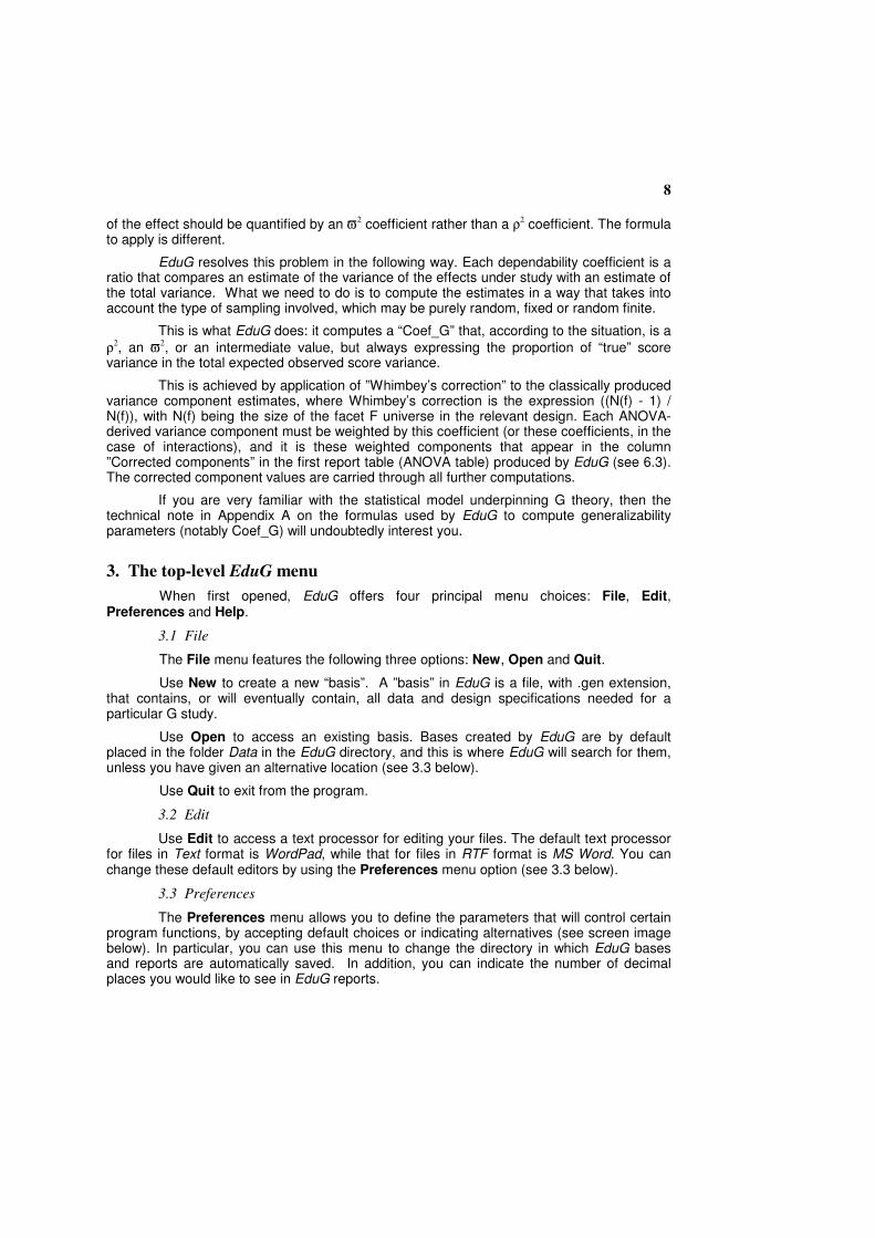
To provide a concrete example of how an observation design is declared in the Work screen, the screen image below shows how the facet lines (top left of Work screen) would be filled for the design proposed by Brennan under the name of “Synthetic Data Set 4” (for a design overview see 8.2). Ten Persons are confronted with the same three Tasks, but success in each task is judged by a different group of four Raters. The design is Px(R:T).
[You will find examples of other observation designs if you open the bases of the folder ForPractice – see section 8.]
12
Reducing your observation design
At some point, you might want to analyze a particular subset of your data, perhaps to look separately at boys and girls, or to compare results for students in different age groups, or simply to exclude a category whose data you consider of questionable validity.
You can do this through the Work screen, by checking the box titled Observation design reduction next to the facet(s) concerned. In response, EduG will list the observed levels for the indicated facet(s), and you will simply need to identify those levels that you wish to exclude, by selecting them with the combination Ctrl + Click (with some operating systems you will have to use Alt + Click or Cap + Click). You can reverse your level selection in the same way.
The observations associated with the facet levels that you have identified in this way will remain excluded from further analysis until you clear the Observation design reduction box(es) once again.
4.3 Declaring your estimation design
Declaring your estimation design simply means declaring your facet universe sizes, i.e. indicating how many levels there are in each facet’s population. For fixed facets, the number of universe levels will be the same as the number of observed levels, since there will have been no level sampling – all the levels of the facet are included in the data set. Otherwise, the number of universe levels will be larger than the number of observed levels. Indicate an infinite facet population with ‘INF’, or even more simply with the letter “i”.
Remember that how you define your facet universes will affect the degree to which your results can be generalized. In particular, if you are analyzing the scores achieved by students on a series of test questions, and if you are interested in establishing the reliability of the students’ average test scores, then you have a choice to make. You could consider the facet Questions as a fixed facet, in which case you would not be able to generalize your findings beyond that particular set of questions. Alternatively, you could consider the facet Questions as a random facet, with a finite or an infinitely sized universe, in which case you could generalize your particular results to that broader set of similar questions, only some of which you happen to have used.
In the example used in section 4.2 to illustrate the declaration of an observation design, note that the facet Tasks is fixed: the number of tasks in the universe is given as three – the same number as are included in the data set.
13
4.4 Declaring your measurement design
You define your measurement design by first identifying which facets are differentiation facets before then identifying (by default) which are instrumentation facets, using a forward slash to separate the one set from the other.
All facets declared in the observation design must appear in the measurement design.
Even if you have reduced a facet to one level only, essentially eliminating it as a source of variation, it must be included in the measurement design.
When identifying facets in your measurement design, you need only use the facet’s unique identifying letter – there is no need to use colons to indicate nesting relationships, since such relationships have already been identified in your observation design. For example, if, in the design Students x Questions, the facet being differentiated is Students, then your measurement design is written as S/Q.
If the Students are nested within Classes, then your measurement design will be SC/Q. If, on the other hand, you are interested in differentiating the Questions, not the Students or Classes, then your measurement design would be Q/SC.
If you have more than one differentiation facet and/or more than one instrumentation facet, the order in which you identify these to the left or right of the slash is not important: SC/QP, SC/PQ, CS/QP and CS/PQ are equivalent.
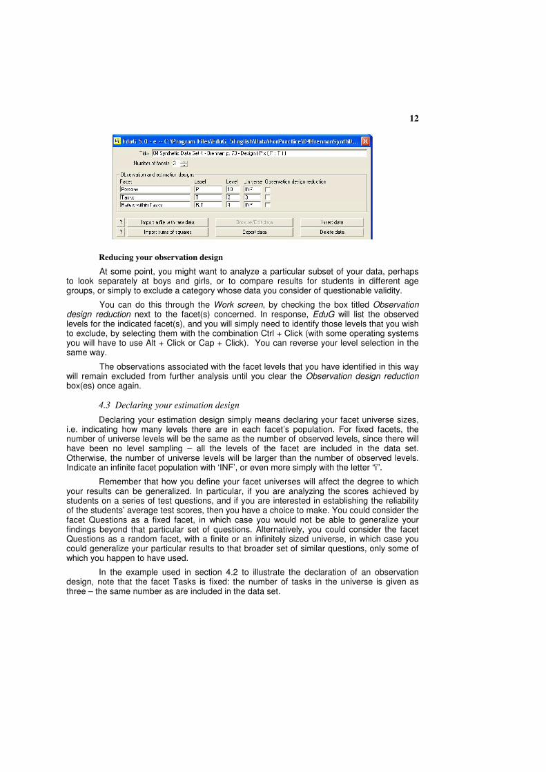
You should enter your design notation in the measurement design box in the middle left of the Work screen.
In Brennan’s “Synthetic Data Set 4”, declared in the Work screen above (see 4.2) and specified in section 4.3, the objects of study are Persons and the conditions of observation are Tasks and Raters within Tasks, with the corresponding measurement design indicated as below:
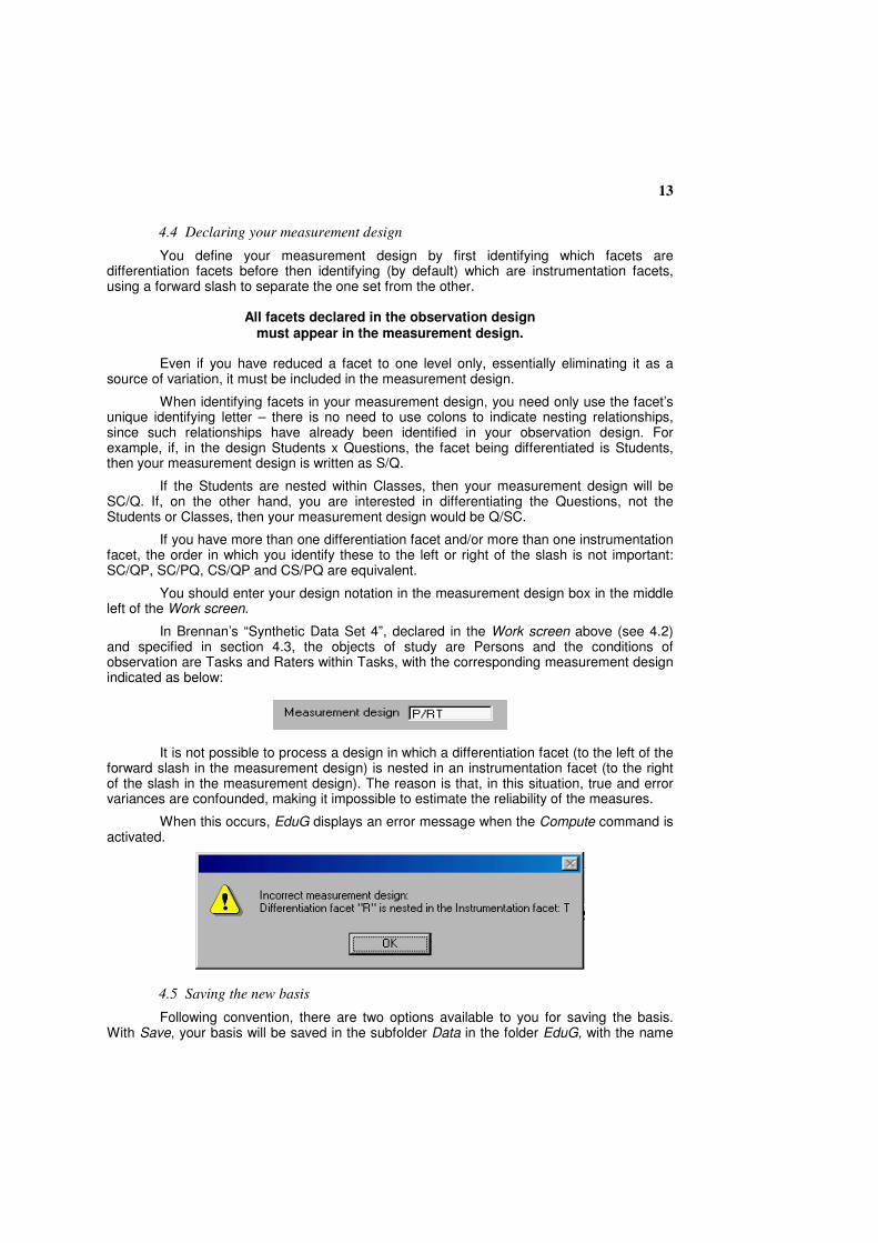
It is not possible to process a design in which a differentiation facet (to the left of the
forward slash in the measurement design) is nested in an instrumentation facet (to the right of the slash in the measurement design). The reason is that, in this situation, true and error variances are confounded, making it impossible to estimate the reliability of the measures.
When this occurs, EduG displays an error message when the Compute command is activated.
4.5 Saving the new basis
Following convention, there are two options available to you for saving the basis. With Save, your basis will be saved in the subfolder Data in the folder EduG, with the name

14
that you had previously given to it. Save as allows you to save the basis with a different name and in a different folder.
If you do not change the name of the file,
it cannot be moved out of the folder in which it was created.
In one way or the other, you should save the basis at this point, even if it does not yet contain any data, or is only partially filled.
5. Managing your data
5.1 Data characteristics
EduG can process raw score data or data already pre-processed into the form of sums of squares and degrees of freedom, and you can enter your data directly into the basis via the keyboard (see 5.2) or alternatively by importing a data file (see 5.3).
If you are to analyze raw score data, then an important constraint is that the data must be complete (no missing data) and balanced, since EduG cannot handle unbalanced designs. Data are balanced when, in a design involving nested facets, there is the same number of levels of the nested facet in every level of the nesting facet. For example, in the simple design Qx(S:C), where Students are nested within Classes, there should be response data for the same number of students in every class.
If your data are unbalanced, for example if you have data for different numbers of students in the different classes, then you will need to impose balance before you add the data to your basis, by deleting records (students and/or classes) as appropriate.
Alternatively, since ANOVA software exists that can compute approximate values for sums of squares and degrees of freedom in such situations, you could avoid the problem by having sums of squares computed elsewhere, and then submitting these, along with degrees of freedom, to EduG for a G study analysis.
The facility to input sums of squares (and degrees of freedom) also allows you to carry out a G study on the basis of a published ANOVA table of results, when you don’t have access to the original data.
5.2 Keying your data
One way to add data to the basis is via the keyboard. On clicking Insert data in the Work screen the following option box will appear, allowing you to indicate the type of data you want to key:
Whichever form of data you choose to enter, your observation design (facet declaration) must already have been defined in the Work screen, otherwise EduG will be unable to identify the nature of the data points you are intending to key in.
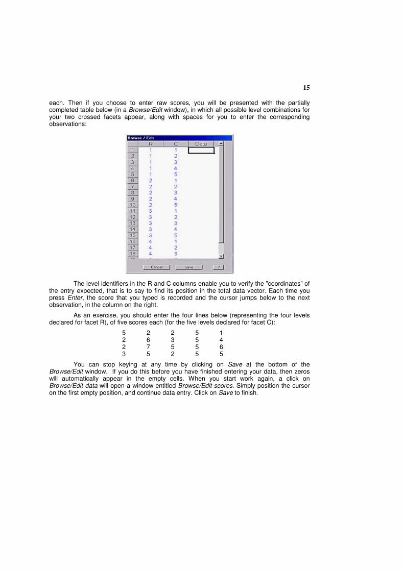
Suppose you have declared an observation design involving two crossed facets, R (here simply indicating “Rows”) and C (”Columns”), with, respectively, four and five levels
15
each. Then if you choose to enter raw scores, you will be presented with the partially completed table below (in a Browse/Edit window), in which all possible level combinations for your two crossed facets appear, along with spaces for you to enter the corresponding observations:
The level identifiers in the R and C columns enable you to verify the ”coordinates” of the entry expected, that is to say to find its position in the total data vector. Each time you press Enter, the score that you typed is recorded and the cursor jumps below to the next observation, in the column on the right.
As an exercise, you should enter the four lines below (representing the four levels declared for facet R), of five scores each (for the five levels declared for facet C):
5 2 2 5 1 2 6 3 5 4 2 7 5 5 6 3 5 2 5 5
You can stop keying at any time by clicking on Save at the bottom of the Browse/Edit window. If you do this before you have finished entering your data, then zeros will automatically appear in the empty cells. When you start work again, a click on Browse/Edit data will open a window entitled Browse/Edit scores. Simply position the cursor on the first empty position, and continue data entry. Click on Save to finish.

16
If instead of Scores? you select Sums of Squares?, this window will open:
All components of variance relevant to the declared observation design are listed in the first column and the associated degrees of freedom in the third. You simply have to introduce the appropriate values of sums of squares in between, in the middle column. For this illustrative exercise, the sums of squares and degrees of freedom are the following:
R 10 3 C 16 4 RC 30 12
If in the estimation design you declare that Rows and Columns are infinite sets, i.e. random facets, and if you offer the measurement design R/C, you will obtain two values for Coef_G (relative and absolute) equal, respectively, to 0.250 and 0.225.
5.3 Importing a data file
Instead of keying your data into the basis, you might prefer to import an existing data file, or to create a data file outside EduG. Again, the data can be raw scores or sums of squares – simply choose one or other of the Work screen commands Import a file with raw data or Import sums of squares. In response, a window will open, inviting you to identify the name and location of the data file you want to import.
Whether it contains raw scores or sums of squares (and degrees of freedom), the file you intend to import must satisfy two conditions:
1) the number of records in the file must correspond exactly to what is expected from the observation design. If the file contains raw scores, their number must correspond to the product of the observed levels declared in the observation design; if the file contains sums of squares, there must be as many rows as independent sources of variance in the ANOVA table.
2) a semi-colon or tab must have been used as delimiter.
If condition 1 is violated, an error message will suggest that you check and correct the offending data file. If condition 2 is violated, EduG will invite you to clarify whether the file is in fixed format or is delimited (see the screen image below).

17
If the file is in fixed format, you will need to indicate the maximum length of the data points. If the file is in free format, then you will need to identify the delimiter that has been used. If you need to check the structure of the file, click See the file to browse it.
If you are to create a data file that you will later import, then it is better to prepare your data file as an Excel or Word table. Identify the rows and the columns (facet names and level identifiers) to facilitate the introduction and validation of the data. The third facet, the fourth, and so on, will be introduced as subdivisions of the rows and columns used for the first two facets.
Col 1 Col 2 Col 3 Col 4 Col 5
Row 1 5 2 2 5 1
Row 2 2 6 3 5 4
Row 3 2 7 5 5 6
Row 4 3 5 2 5 5
Once the table is completed and verified, you should eliminate the row and column
headings, retaining only the raw data, as shown below:
5 2 2 5 1
2 6 3 5 4
2 7 5 5 6
3 5 2 5 5
Save the file in Text only format (ASCII), with tabs as delimiters, and with suggested file extension .txt. (Check that the number of lines in the file is correct – sometimes a last line, containing a paragraph sign, will need to be deleted). Once saved, this table will take the form of a vector, that is equivalent to the column of values that you might otherwise have keyed directly into the Browse/Edit window shown in section 5.2.
If you intend to import a file containing sums of squares and degrees of freedom, then the file should contain one record (i.e. one row) for every source of variance, identifying the variance source and recording the relevant sums of squares and degrees of freedom. Data points should be delimited with tabs or semi-colons as usual. For instance, for the above exercise, the file with semi-colon delimiter would look like this:
R;10;3 C;16;4 RC;30;12
18
Row order is not important – it will have no influence on the computations – but EduG must be able to recognize each source of variation (where problems arise an error message will appear)
The file should have been saved in Text only format, with suggested extension .dat.
5.4 Editing data
Use Browse/Edit data in the Work screen to examine the data that you have saved in the basis. Use the vertical scroll bar, as necessary, to move through the file. To change an observation, simply position the cursor on the old value and type in the new value. When all changes have been made, re-save the file.
5.5 Exporting data
The Work screen option Export data lets you save the data currently in the basis as an ASCII file (Text format only), with a file name of your choice
5. The data will be saved in
whichever form they were originally imported, i.e. as raw scores or sums of squares.
To choose an appropriate and unique name, you might want to overview the names of pre-existing data files. You can do this by clicking on the icon in the centre of the Reports area, next to File, at which a window will open giving you an opportunity to inspect the content of the relevant directory.
5.6 Deleting data
Once you have exported data out of the active basis, you can then delete the data from the basis by clicking on Delete data, and confirming your intent in response to the prompt. You should then save the modified basis. Once the basis is empty of data, you can modify the observation design and then import a new data set.
6. Requesting analyses and interpreting reports
6.1 Analysis possibilities and report choices
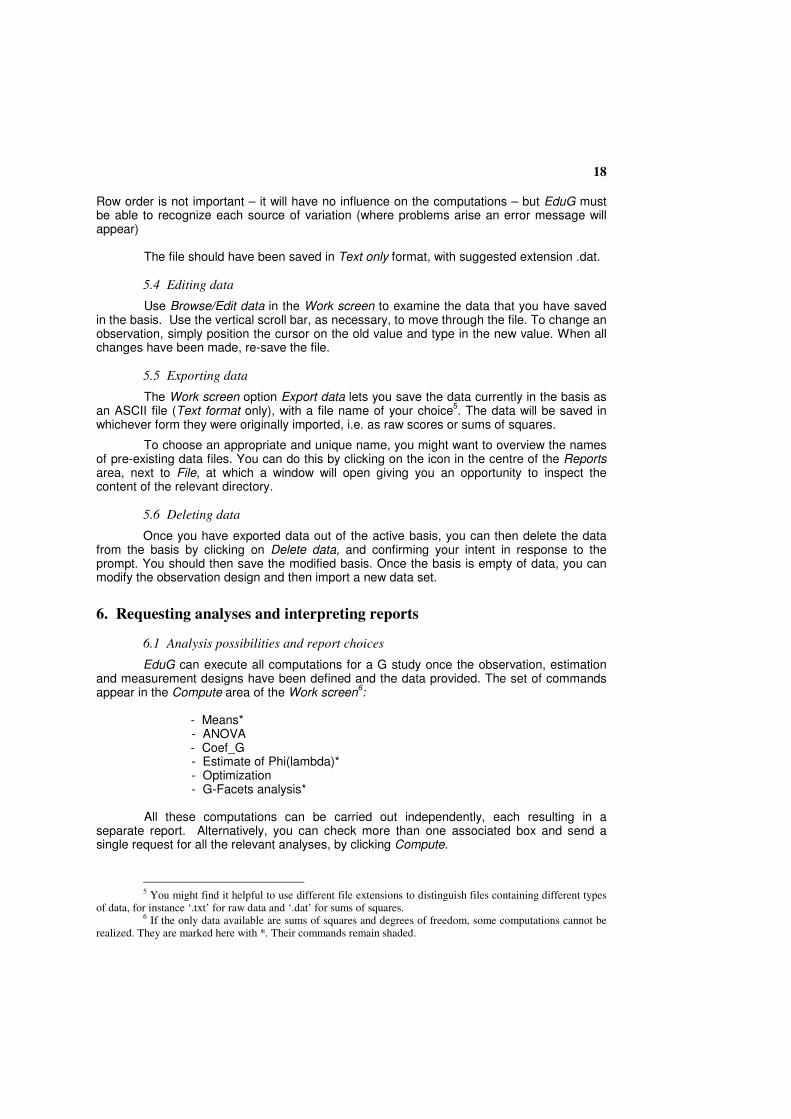
EduG can execute all computations for a G study once the observation, estimation and measurement designs have been defined and the data provided. The set of commands appear in the Compute area of the Work screen6:
- Means* - ANOVA - Coef_G - Estimate of Phi(lambda)* - Optimization - G-Facets analysis*
All these computations can be carried out independently, each resulting in a
separate report. Alternatively, you can check more than one associated box and send a single request for all the relevant analyses, by clicking Compute.
5 You might find it helpful to use different file extensions to distinguish files containing different types
of data, for instance ‘.txt’ for raw data and ‘.dat’ for sums of squares. 6 If the only data available are sums of squares and degrees of freedom, some computations cannot be
realized. They are marked here with *. Their commands remain shaded.
19
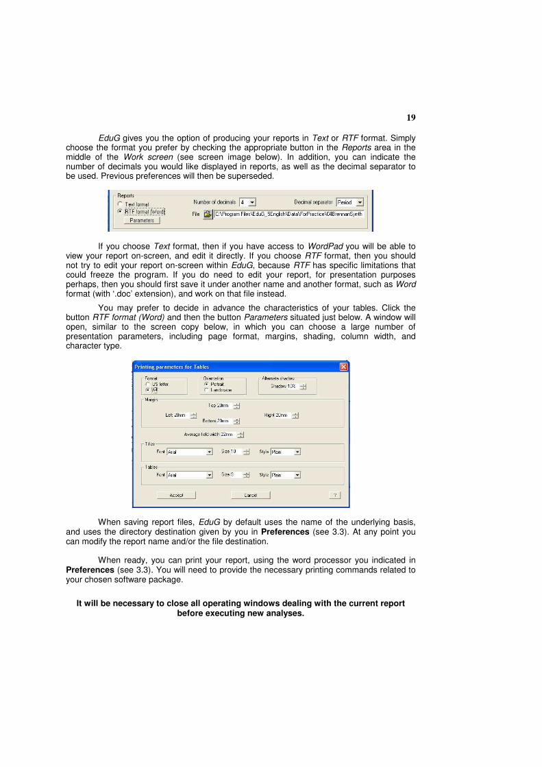
EduG gives you the option of producing your reports in Text or RTF format. Simply
choose the format you prefer by checking the appropriate button in the Reports area in the middle of the Work screen (see screen image below). In addition, you can indicate the number of decimals you would like displayed in reports, as well as the decimal separator to be used. Previous preferences will then be superseded.
If you choose Text format, then if you have access to WordPad you will be able to view your report on-screen, and edit it directly. If you choose RTF format, then you should not try to edit your report on-screen within EduG, because RTF has specific limitations that could freeze the program. If you do need to edit your report, for presentation purposes perhaps, then you should first save it under another name and another format, such as Word format (with ‘.doc’ extension), and work on that file instead.
You may prefer to decide in advance the characteristics of your tables. Click the button RTF format (Word) and then the button Parameters situated just below. A window will open, similar to the screen copy below, in which you can choose a large number of presentation parameters, including page format, margins, shading, column width, and character type.
When saving report files, EduG by default uses the name of the underlying basis, and uses the directory destination given by you in Preferences (see 3.3). At any point you can modify the report name and/or the file destination.
When ready, you can print your report, using the word processor you indicated in Preferences (see 3.3). You will need to provide the necessary printing commands related to your chosen software package.
It will be necessary to close all operating windows dealing with the current report before executing new analyses.

20
6.2 Means and variances
On request, EduG will compute the mean of the observations for each level of each facet (such as Classes, Students and Questions) and for each facet interaction (for example, Classes by Questions).
To request these computations, simply click on Means and then select the source of variation that interests you from within the presented list (see below).
_
Use Control, or Alt, or Cap, depending on the operating system, to select more than one source of variance. The same procedure reverses your selection. Once you have finalized your selection, click on Compute to launch the calculations. The results are presented on screen by the text editor that you requested (see 6.1).
Each mean is accompanied by the variance of the n values that have been averaged. Note that the formula used for computing the variance puts n in the denominator, and not (n-1), because it is a descriptive sample statistic that is required and not a population estimate.
Other important means and variances are computed by EduG. On the last line of the G study report the grand mean is shown, i.e. the overall mean of all the values in the data set (or at least all those not excluded by a reduction of the observation design). This mean is immediately followed by its sampling variance, estimated on the basis of the observed sample.
To compute this variance, the corrected components of variance (see 2.3) for all sources of variation in the estimation design are added, each divided by the number of times that the facet or facet interaction concerned has been sampled (the number of observed levels of the facet, or of level combinations in the case of an interaction of facets). The only facets excluded from this calculation are fixed facets, since these are not sampled and do not therefore contribute to sampling variation.
As usual, the square root of the sampling variance of the grand mean gives the standard error of this mean. This standard error may be used to establish a confidence interval containing the true mean for all sampled universes (under Normal distribution assumptions).
For interested readers, the exact computation algorithm is presented in this frame.
Due to sampling fluctuations, the estimate of the grand mean does vary. Its variance is the sum of the corrected components of variance (see 2.3), each one divided by the number of times it has been observed (the facet’s size for a main effect and the product of the facets’ sizes for interactions).
All these quotients add up to the grand mean’s variance when all facets are infinite random. But it is not always the case that all the facets are infinite random. This is
Commentaire [s1] :

21
why each quotient must still be multiplied by a “finite population correction factor”, the formula of which is (N-n)/(N-1) when a classical definition of variance is being used, as is the case here.
It is clear that this correction factor reduces to zero when the facet is fixed, (with N = n) and it is equal to 1 when the facet is infinite. For random finite facets, (with n < N), the coefficient of correction has an intermediate value. Thus the sampling variance of the grand mean can be obtained for any random sampling design.
The procedure can be generalized. By successively reducing the observation design (for instance to girls and then to boys), the mean (and its standard error) can be obtained for each group, yielding a confidence interval for the difference of their means. This procedure is post hoc, however, admitting that the two sets are fixed and limited to the groups observed. But some other facets are sampled and EduG tells us what influence their random effects may have had. If a “prospective” confidence interval is needed, for two randomly chosen objects of measurement, then the facet Gender has to be declared an infinite random facet, as is implicitly done when statistical tests, like the “t” and “F” tests, are computed.
6.3 Analysis of variance
The brief description of Coef_G given in section 2.3 should suffice to show that the algorithm for computing the variance components represents the essence of the EduG software. The formulas that have been used were presented by Jean Cardinet and Linda Allal in Fyans (1983). Essentially, they follow those developed by Robert Brennan (1983, 1992), except for the choice of a classical definition of variance (which, however, affects only the estimates for fixed and finite universes, as explained in Appendix A).
To request an ANOVA or a G study (or both), check the appropriate box(es) in the Compute area towards the bottom left of the Work screen, and then, or later, click Compute to start the computations.
In the Work screen below, you will see that an ANOVA and a G study are ready to be launched, for “Synthetic Data Set 4”, the Brennan example whose observation and estimation designs were given in sections 4.2 and 4.3 (the facet Tasks was declared fixed, with a universe of size 3).
In response to the request, EduG first displays the relevant observation and estimation designs, before presenting the associated ANOVA results (see below).

22
The ANOVA table is conventional, save for one EduG addition in the form of the ”Corrected Components” column, which presents variance component values after application of Whimbey’s correction (see 2.3).
Some components can be problematic. In particular, while in theory they are not possible, sampling fluctuations around small component values sometimes result in negative component estimates. These estimates are then presented for information in the ANOVA table with their negative sign, but they are replaced by zeros in the follow-on computations of the generalizability parameters.
Other components have necessarily null values, such as those derived from a one-level facet (typically resulting from an observation design reduction – for example to one gender only). In this case, a row of dots represents the null values, and again a zero value is carried through ensuing calculations. No null value appears in the case of this example.
The ”%” column shows the proportion of the variance of individual scores (estimated as the sum of the corrected components) that is attributable to each variance source (i.e. to each corrected component). Cronbach advised that these percentages should not be interpreted as directly reflecting the relative importance of each variance source, since real life decisions are generally made on the basis of total scores or mean scores, and not on the basis of non-summarized data points. The relative importance of each source of error in the total error variance is rather given in the G study table that follows.
In the Standard Error (SE) column are estimates of the standard errors associated with the various estimated variance components. They may be used to establish confidence intervals to test the significance of these components. However, the standard errors in question refer to components in a completely random effects model (those of column 5, rather than those of column 7). Here the information given by the software should be considered as indicative only.
If you erase the check mark placed by default against “ANOVA” in the Work screen, the usual ANOVA table will not be printed (although it will be computed as usual). In this way you can avoid printing the same ANOVA table repeatedly when several different G studies are requested, based on the same data.
6.4 G study
23
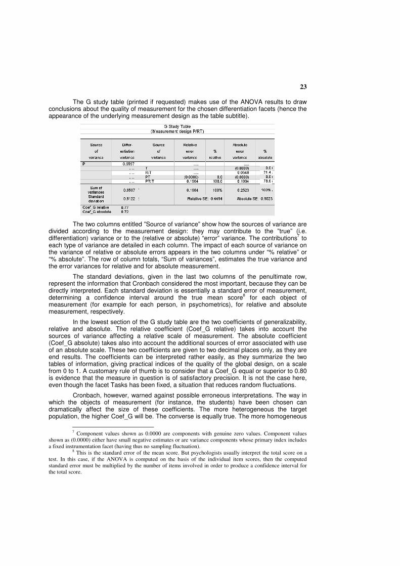
The G study table (printed if requested) makes use of the ANOVA results to draw
conclusions about the quality of measurement for the chosen differentiation facets (hence the appearance of the underlying measurement design as the table subtitle).
The two columns entitled ”Source of variance” show how the sources of variance are divided according to the measurement design: they may contribute to the ”true” (i.e. differentiation) variance or to the (relative or absolute) “error” variance. The contributions
7 to
each type of variance are detailed in each column. The impact of each source of variance on the variance of relative or absolute errors appears in the two columns under “% relative” or “% absolute”. The row of column totals, “Sum of variances”, estimates the true variance and the error variances for relative and for absolute measurement.
The standard deviations, given in the last two columns of the penultimate row, represent the information that Cronbach considered the most important, because they can be directly interpreted. Each standard deviation is essentially a standard error of measurement, determining a confidence interval around the true mean score
8 for each object of
measurement (for example for each person, in psychometrics), for relative and absolute measurement, respectively.
In the lowest section of the G study table are the two coefficients of generalizability, relative and absolute. The relative coefficient (Coef_G relative) takes into account the sources of variance affecting a relative scale of measurement. The absolute coefficient (Coef_G absolute) takes also into account the additional sources of error associated with use of an absolute scale. These two coefficients are given to two decimal places only, as they are end results. The coefficients can be interpreted rather easily, as they summarize the two tables of information, giving practical indices of the quality of the global design, on a scale from 0 to 1. A customary rule of thumb is to consider that a Coef_G equal or superior to 0.80 is evidence that the measure in question is of satisfactory precision. It is not the case here, even though the facet Tasks has been fixed, a situation that reduces random fluctuations.
Cronbach, however, warned against possible erroneous interpretations. The way in which the objects of measurement (for instance, the students) have been chosen can dramatically affect the size of these coefficients. The more heterogeneous the target population, the higher Coef_G will be. The converse is equally true. The more homogeneous
7 Component values shown as 0.0000 are components with genuine zero values. Component values
shown as (0.0000) either have small negative estimates or are variance components whose primary index includes a fixed instrumentation facet (having thus no sampling fluctuation).
8 This is the standard error of the mean score. But psychologists usually interpret the total score on a
test. In this case, if the ANOVA is computed on the basis of the individual item scores, then the computed standard error must be multiplied by the number of items involved in order to produce a confidence interval for the total score.
24
the population, the more difficult it will be to differentiate between its members. It could be the case here.
A similar warning concerns the usefulness of a measurement design. Usefulness does not depend solely on the generalizability of the measure, but depends also on the amount of supplementary information brought by the instrument, considering that other sources of information already exist. Coef_G is thus more difficult to interpret than is the error of measurement.
Then again, to evaluate validly the computed margin of error in a measurement procedure, you should realize that other sources of non-sampled random fluctuation could be at play. Few designs can introduce into a G study the entire range of possible factors that might contribute to error variance.
The sampling variance of the grand mean, given at the end of the report, is essentially used to compute the domain referenced Phi(lambda) coefficient (see 6.5). But its square root, the standard error of measurement of the grand mean, can also be a basis for judging the precision of the observed mean performance.
6.5 Phi(lambda) coefficient
In response to the Work screen command Estimate of Phi(lambda), EduG produces a coefficient of generalizability for absolute measurement that takes into account the object of interest in many educational assessments, viz. the difference between the score reached by a student and the cut score separating success, or mastery, from failure.
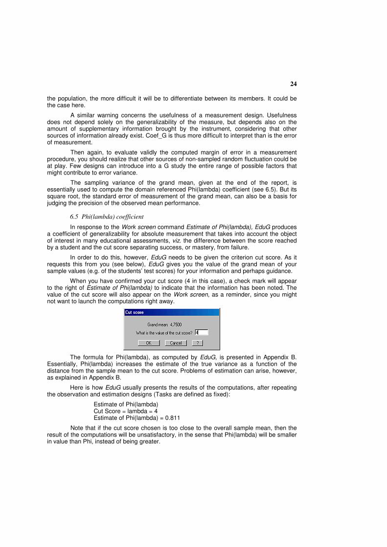
In order to do this, however, EduG needs to be given the criterion cut score. As it requests this from you (see below), EduG gives you the value of the grand mean of your sample values (e.g. of the students’ test scores) for your information and perhaps guidance.
When you have confirmed your cut score (4 in this case), a check mark will appear to the right of Estimate of Phi(lambda) to indicate that the information has been noted. The value of the cut score will also appear on the Work screen, as a reminder, since you might not want to launch the computations right away.
The formula for Phi(lambda), as computed by EduG, is presented in Appendix B. Essentially, Phi(lambda) increases the estimate of the true variance as a function of the distance from the sample mean to the cut score. Problems of estimation can arise, however, as explained in Appendix B.
Here is how EduG usually presents the results of the computations, after repeating the observation and estimation designs (Tasks are defined as fixed):
Estimate of Phi(lambda) Cut Score = lambda = 4 Estimate of Phi(lambda) = 0.811
Note that if the cut score chosen is too close to the overall sample mean, then the result of the computations will be unsatisfactory, in the sense that Phi(lambda) will be smaller in value than Phi, instead of being greater.

25
An example is given by the design P/RT considered earlier, with Tasks fixed, where
the value of Phi (i.e. Coef_G absolute) is equal to 0.723. When a cut score of 4.5 is applied, Phi(lambda) is equal to 0.698 only. In such a case, EduG will replace Phi(lambda) by Phi (Coef_G absolute), which is theoretically its lower bound. The following type of information is displayed:
Estimate of Phi(lambda) Cut Score = lambda = 4.5 Restricted estimate of Phi(lambda) = 0.723 Raw estimate of Phi(lambda)= 0.698
6.6 Optimization
Your G study analysis will reveal which sources of variation are contributing the most to error variance and which are contributing the least. This is the information you need for identifying how to improve your measurements in the future. EduG cannot automatically identify the optimal observation design for your particular measurement application. But it does provide you with a tool for identifying the optimum design yourself, through successive approximations.
The optimization facility allows you to vary the numbers of observed levels for one or more instrumentation facets, and to see the potential effect of the change on measurement reliability. You should, where possible, increase the numbers of observed levels of the greater contributors to error variance and, if it contributes to cost-effectiveness, decrease the numbers of observed levels of those instrumentation facets that contribute little to the error variance.
As an example, suppose that you want to try alternative combinations of facet levels for the measurement design discussed earlier, viz. P/RT with T fixed. To do so, you would simply check the Optimization box in the Compute area of the Work screen. In response, you would be presented with a grid ready to receive up to five different observation and estimation designs (five “Options”). Clicking on Copy would reproduce under Option 1 the current observation and estimation designs. You can modify the number of observed levels of the instrumentation facets, to re-define Option 1. Clicking again on Copy would reproduce these new values under Option 2, to be modified again. Each option is in fact the basis for the following one (although this need not be the case).
T being fixed here, the size of the sample and of the universe for T will both remain at 3. But you can modify the number of raters for each task. You are allowed up to five possible choices of facet level numbers. You might try 2, 3, 4, 5, and 6 raters for each task, as shown below:
What you will not be able to do is change the number of levels of any of your differentiation facets (the single facet P in the example above), although you will be able to change their universe sizes if you wish.

26
Clicking on Compute will produce the Optimization results table below, in which the
original and combination values are noted and the resulting coefficients, variance and error estimates are presented:
The results agree with those of Brennan (2001, p.147). They show that with five raters per task, it is possible to differentiate reliably between persons (Coef_G relative = 0.806). On the other hand, for an absolute scale of measurement, five raters would not quite be satisfactory. At least six raters would be needed (Coef_G absolute = 0.797).
Although the facet Tasks has thus far been considered as fixed, you might alternatively consider that the three tasks are a sample drawn from a large set of other possible tasks. You could then look for the optimum combination of tasks and raters. After changing the estimation design in the Work screen of EduG, you could ask for another Optimization window. You could try the following combinations that leave the total number of observations approximately constant:
The results are presented in the following table:

27
Clearly, option 5 produces, within the same overall number of observations, the best generalizability coefficients, higher than for any other combination of facet levels and higher than the observed original values, both for relative and for absolute measurement. This increase in reliability would be achieved by increasing from 3 to 6 the number of tasks attempted by each person and reducing from 4 to 2 the number of raters per task.
6.7 G-Facets analysis
G-Facets analysis generalizes item analysis, a standard procedure in psychometrics. Its objective is to compare the values of the G coefficients that are obtained when each of the levels of the facet under study is in turn excluded from analysis.
On checking the G-Facets analysis box in the Compute area of the Work screen, you will be offered a list of all your instrumentation facets, or at least all instrumentation facets that are not nested in others – see the screen image below, which shows that there is only one such facet with the design Px(R:T).
From within the list you should identify the facet for which you want to conduct a G-Facets analysis, simply by clicking on it. Use CTRL + Click if you want to select several facets simultaneously (with some operating systems, you must use the Cap and/or Alt key while clicking). Use the same procedure to de-select facets. Differentiation facets are, by definition, not amenable to a G-Facets analysis, since they contribute only to true score variance. Nested facets will also not be included in the facets list, since “level 1”, ”level 2”, etc, of a nested facet differ in meaning from one level of the nesting facet to another (think again of students within classes).

28
When you have identified and confirmed the facets you want included in the G-
Facets analysis, a checkmark will appear on the Work screen, to the left of G-Facets analysis, and the facets chosen are noted next to it for information. As soon as you click Compute the analysis will begin, and the respective report will be produced.
The report itemizes the various levels of each relevant facet, and presents against each level the values of the two coefficients of generalizability, relative and absolute, that arise when that level is eliminated from the analysis. In the present example of the Px(R:T) design with T fixed, there was only one facet to analyze, Tasks, with only three levels. The results are given in the table below:
The evidence is that eliminating the task “level 3” from the analysis would increase measurement reliability considerably. In fact, for relative measurement, the G coefficient that would be associated with a study involving only Tasks 1 and 2 would be the same as that for a study in which five raters instead of four evaluated all three tasks: it would reach 0.80 in both cases. But the number of observations would be eight if we act on the results of the G-Facets analysis, as opposed to 15 if we simply increase the total number of observations. For absolute measurement, a total of eighteen observations would be needed to reach a reliability of 0.80 in one case, while eight would suffice if only Tasks 1 and 2 were used. The economy is striking.
Note that Tasks must be a fixed facet for this strategy to make sense. If it were random, there would be no justification for giving up Task 3 in a D study, i.e. in a future application of the design, because:
1) on the theoretical level, dropping an element judged too heterogeneous would invalidate the representativeness of the sample and hence the validity of the inference;
2) on the practical level, rejecting Task 3, i.e. level 3, would be meaningless if other levels were to be drawn for the next application of the design.
On the other hand, if facet T is fixed, nothing prevents you from modifying its definition to accommodate a change in the list of its admissible levels.
Thus, we conclude that G-Facets analysis can be most useful in identifying levels of fixed facets that might be genuinely flawed in some way and that impair measurement. Here, Task 3 might be flawed.
G-Facets analysis should not be confused with the practice of item analysis in psychometrics. From the point of view of G theory, this classical procedure contradicts the postulate of random sampling from an item domain, and could result in non-valid generalizability results. If you apply this method, the domain from which the resulting items will have been sampled might not be the domain to which you intended to generalize your results.
Nevertheless, the idea (first suggested and programmed by Erreur ! Source du
renvoi introuvable.) of rejecting test items that function differently from the others is, admittedly, an attractive one. If you can discover what it is that characterizes the minority of items that behave differently from the majority, then this might help you to refine your
29
definition of the item universe that you really want to sample in your assessments, at which point you can validly exclude the questionable items.
A new random sampling of items from within this newly defined domain would then be advisable, rather than proceeding with the possibly unexplained set of “best behaved” items.
7. Changing your designs
7.1 Changing your observation design
You can reduce your current observation design by temporarily dropping some levels from any facet, as explained earlier (see 4.2).
This EduG facility enables you to conduct secondary analyses on subsets of your data. You could, for example compare the results for various different social groups or the different effects of controlled experimental conditions, while remaining within the frame of your original observation design.
But you might also, or alternatively, want to analyze your data according to an entirely different observation design from the one you originally declared. You might, for example, want to eliminate a facet entirely, perhaps by confounding nested facets, or you might want to introduce new subgroups as additional levels for an existing facet. You might even want to introduce new facets.
Whatever your motivation, if you want to change your original observation design, rather than simply reduce it, then you will first have to empty the basis of data (see 5.5 and 5.6), before changing the observation design and re-importing the original data set or importing a new one (see section 5.3).
7.2 Changing your estimation design
Your estimation design can be changed easily, without the need to export and then re-import your data, since here you are simply redefining universe sizes.
There are two ways to change a facet’s universe size: 1) simply change the size given earlier in the relevant facet row of the Work screen; 2) check the Optimization box in the Compute area of the Work screen, and change the
relevant universe sizes when these are presented. The consequence of the change will be a modification of the ANOVA model
(random, fixed or mixed model) and consequently a modification of the coefficients used for computing the components of variance. Estimates of generalizability parameters will be different.
Be careful: changing facet universe sizes affects the G study results the first time you click on Compute. This helps when applying a trial and error optimization strategy. But the changes are not permanently recorded unless you save the modified design.
30
7.3 Changing your measurement design
The same data set can be analyzed from several different points of view. You can focus on the results of students, of classes, of schools, or of entire national populations. So there are as many possible measurement designs as there are combinations of facets to be measured, the other facets becoming instrumentation facets in the measurement process. True and error variances will differ in each case and give rise to different measurement reliabilities. Several facets might need to be simultaneously differentiated, just as several facets can together constitute a common universe of generalization.
Suppose, for example, that Students, nested within Classes, attempt a set of items developed to match a given test specification, which crosses content Domains (perhaps History topics) with forms of Presentation (e.g. documents, or verbal questions). If there is only one item in each cell of the specification table, the facet Items is confounded with the interaction Domains x Presentations. The global design is then (S:C) x (DxP). The Items facet is present, but “hidden”.
If you want to differentiate between students, whatever class they are in, using a common measurement scale, then you will be differentiating simultaneously between classes and between students within classes. To estimate the reliability of the assessment you will need to put both facets, Classes and Students within Classes, on the face of differentiation, i.e. you will need to put both on the left of the slash in the measurement design, writing this as SC/DP. If instead you are interested in differentiating between forms of presentation, then the facet Presentations becomes the face of differentiation, all other facets being instrumentation facets. The appropriate measurement design is then P/DSC.
If you want rather to compare the difficulties of the items, then, since the specific effect of each item is confounded with the interaction between Domains and Presentations, the differentiation variance will comprise three components: the interaction between Domains and Presentations, along with the facet Domains and the facet Presentations. The measurement design is thus DP/SC. EduG will compute the G studies corresponding to these three measurement designs: SC/DP, P/DSC and DP/SC (and to several others). The facets which are not objects of measurement will become instruments of measurement and will form the instrumentation face. Later, by fixing or leaving random one or other of these instrumentation facets in turn, you can determine their impact on the precision of your measurements.
You can modify your measurement design without any need to export and re-import the data. You do this through the Work screen, simply by changing the design notation in the Measurement design box.
7.4 Measurement designs with no differentiation aim
Measurement designs typically identify an “object of measurement”, like Students, whose levels you are attempting to differentiate. But there are situations in which differentiation is not the focus of a G study. The aim is rather the estimation of the standard error of measurement of one overall mean, such as the level of anxiety about global warming among young adults in Western Europe, or the numeracy attainment of Grade 7 students in the USA. There is no differentiation facet in such studies, only instrumentation facets.
For EduG the appropriate measurement design is indicated by listing all the observation design facets to the right of the slash, with no facets to the left. For example, suppose we have the observation design described in section 7.3, i.e. (S:C) x (DxP), where S, C, D and P represent, respectively, Strudents, Classes, content Domains and forms of Presentation. And suppose that we are not interested in differentiating among students, either overall or within their classes, but instead want to estimate the population performance

31
of such students on those content domains and with those given presentational forms The new measurement design will be described symbolically as /SCDP. All four facets are considered as conditions of observation affecting the measures.
For such measurement designs, EduG produces a G study table in which all random facets and their interactions are shown as sources of error, quantified in the “absolute error variance” column. The sum of these variance contributions (the column total) corresponds to the sampling variance of the grand mean. With its square root, the standard error of measurement, you can compute a confidence interval within which lies the true mean (under Normal distribution assumptions).
With the optimization module, you may then, as usual, explore the expected effect of various changes in the sampling design. A general rule of thumb is to observe more levels of the facets with a large variance, and in compensation, to reduce the size of the samples when conditions seem to be less influential. By successive approximations, an optimum combination of sampling strategies can be identified.
8. Exemplification
8.1 The folder Data and the sub-folder ForPractice
When EduG is installed, a folder is created in the Data directory with the name ForPractice. The folder contains 16 pre-created bases. The bases contain data, but the design details remain to be declared, and the analyses launched by clicking the Compute button. The principal purpose of the bases is to give new users an opportunity to use EduG right away, to familiarize themselves with what it offers and to discover its interpretation possibilities. You will be able to compare results for different commands.
Some of the examples, like Brennan’s (2001) ‘Synthetic Data Sets’, are purely numerical exercises. They are nevertheless useful for comparing the outputs of different programs, among them EduG and GENOVA. Other examples are real, but have been de-contextualized, since they are here simply to illustrate methodology: they serve to demonstrate the various types of situation and design that EduG can handle. Although primarily offered for practice purposes, the bases can potentially contribute towards other objectives as well. In particular, the examples illustrate how measurement designs that are much more complex than those typically considered in student textbooks can be described and processed.
One of the most difficult tasks for those new to the field is that of identifying those facets that are at play in a measurement situation, and determining the nature of their inter-relationships in terms of crossings and nestings. Working with the variety of examples represented in the illustrative bases should serve to clarify this particular issue. Those researchers with experience of applying G theory in a psychometric context will be interested to see examples of application in other fields, notably in an experimental setting or in the context of international attainment surveys.
The 16 example bases are held in the special folder ForPractice in order to keep them separate from the real data you will introduce when working with EduG. You can erase the folder ForPractice when you no longer need it.
8.2 The illustrative data sets
In this overview, the data sets are ordered from the simplest to the most complex, each identified by the name of the basis that contains it. References are given in full in the bibliography.

32
01BrennanSynthData1 The first example presents Synthetic Data Set 1, from Brennan’s Generalizability
Theory (Brennan, 2001, page 28). Ten people answered 12 questions (items), and scored 0 for a wrong answer and 1 for a correct one. This is the basic two-facet crossed design (PxI, equivalent to the SQ design that has been mentioned on page 4 of this User Guide) that features in both classical psychometrics and G theory, but which the latter can take further, as in the examples that follow.
02BrennanSynthData2 The data set for the second example comes from the same book (Brennan, 2001,
page 43). In this design, (I:P), Items are nested within Persons, as in an oral examination where the questions (items) differ from one candidate to another.
03BrennanSynthData3 Design 3 is a three-facet crossed factorial design, with Persons crossed with Items
and Occasions (P x I x O). Data were copied from Table 3.1 of the same book (Generalizability Theory, Brennan, 2001, page 72).
04BrennanSynthData4 Design 4 is more complex [P x (R:T)]. In this case, ten persons are confronted with
the same three tasks, but success in each task is judged by a different group of four raters. The data to be analyzed are those on page 73 of Generalizability Theory. EduG users will certainly want to compare their results with those given in this standard manual (Brennan, 2001, page 116 for the random effects D study and page 147 for the design with Tasks fixed).
05TermPapers This example is also drawn from a handbook (Bertrand & Blais in 2004), in which the
data are presented on page 75. It is a three-facet crossed design, since ten students have each written essays about two different topics and their essays are evaluated by three different raters. In itself, this design is no different from Brennan’s third example, but its special interest comes from the fact that it can be compared with Example 6.
06TermPapersSSQ The design here is exactly the same as the previous one, but the data available this
time are sums of squares and degrees of freedom for each source of variance. You will see from this example that most of the conclusions of a G study can be obtained on the basis of these intermediary results, with rare exceptions that are worth looking out for.
07ClassObservation G theory can also be applied to frequency data, if these can be considered as
scores derived from an observation instrument. This is the case for Example 7, drawn from the same handbook by Bertrand and Blais (2004, page 77). Five teachers are each observed by a different pair of raters (school inspectors), who record the number of questions that the teacher poses to pupils in one hour of classroom activity. These ”Judges” visit the classrooms at five different randomly chosen moments. Thus, here, Occasions (of visit) are nested within Judges, who in turn are nested within Teachers. The observation design is O:J:T.
08Depressionscale Several of the following examples are taken from a series of exercises prepared by
Bain and Pini (1996). The first focuses on computation of the reliability of a Depression scale. The design P x I, Patients by Items, is elementary and presents no difficulty. The example,

33
though, represents an opportunity for experimenting with EduG’s various options, such as a G-Facets analysis with a reduced observation design, achieved by temporarily excluding some items or some patients.
09Interview In Bain and Pini’s second example (page 67), 120 employees of a large firm are
interviewed by two psychologists, and rated on four personality traits for purposes of a possible promotion. Thus, the design crosses 120 employees, two interviewers and four personality dimensions. This is a chance to focus on the standard error of each individual’s mean and its resulting confidence interval. You can use the option Optimization to see whether a greater number of interviewers might appreciably improve the reliability of employee ranking.
10AttitudeChange In the third example drawn from the Bain and Pini handbook (page 71), the G study
is intended to indicate whether the researchers’ experimental design can be used to reliably measure attitude change following participation in a course of training. Four facets are considered: Subjects, nested in experimental Groups, Moments (before and after training) and the Items of the attitude scale used. You can compare the values of Coef_G, relative and absolute and look for the reason for their difference.
11TeachingWriting This exercise (drawn from Bain & Pini, page 75) aims to evaluate the effectiveness
of a new method for teaching essay writing, by comparing the results of an experimental student group with those of a control group, using three skills criteria. You can suggest several different measurement designs, especially if you want to explore the influence on performance variance of the facets in which the students are nested.
12Mathematics This study (Bain & Pini, p. 80) compares the relative difficulties of 10 problems
(items) featuring fractions. The test is in two versions (forms), both containing the same items but in a different random order. Each pupil receives only one version. Pupils belong to one of two different streams. The observation design has four facets, one of which is nested in the interaction of two others – a common design in G studies.
13ReadingTestIEA This example is typical of applications of G theory in the field of attainment surveys.
After a pilot study to quantify the influence of different sources of variance on attainment variation comes the optimization step, with which you can try to identify the most appropriate design for maximizing the generalizability of the intended attainment comparisons.
14Physics A group of Physics teachers wants to measure the effect of certain factors on pupil
learning. They set out to analyze their pupils’ test results in terms of topics studied and levels of objectives, separately for boys and girls. Their observation design, with five facets, leads to a kind of attainment survey of their own pupil population.
15MathSurvey The purpose of the G study was to check the accuracy of the estimated mean level
of achievement in mathematics for the whole population of school leavers in a given region. The standard error of measurement for the grand mean permits establishment of a confidence interval around the ”true” grand mean of this population.

34
16LanguageLearning This observation design was used to test the results of EduG in the limiting case
where eight facets are taken into consideration. The G study investigated the dependability of a questionnaire for making various comparisons. In particular, the problem was to measure pupils’ attitudes towards the learning of German as a foreign language, and any change in these attitudes (positive or negative) between the beginning and the end of the school year. The design served to identify the influence of several factors (attitude traits, item types, schools, streams and districts) on the quality of measurement, and to explore different strategies for improvement.
8.3 Further G study examples
Many generalizability studies with a didactic objective have been conducted in the field of education, in French-speaking as well as English-speaking countries. You can consult an overview of some of these on the IRDP website, on the pages related to Edumetrics-Generalizability, and in particular at the address:
http://www.irdp.ch/edumetrie/exemples.htm
Future educational applications could usefully be added to those already in the overview, however brief the description, since practitioners can only gain from this information exchange. If, therefore, you have an example to offer at any point, then please submit it to [email protected] for inclusion in the database.
Studies in other fields of application are also referenced, though not accompanied by summaries, in a bibliography that can be downloaded in pdf format from the same site:
http://edumetrie.irdp.ch/bibliographie.htm

35
Bibliography
Abdi, H. (1987). Introduction au traitement statistique des données expérimentales. Grenoble: Presses universitaires de Grenoble, p. 108.
Bain, D. & Pini, G. (1996). La généralisabilité: mode d'emploi. Geneva: CRPP.
Bertrand, R. & Blais, J-G. (2004). Modèles de mesure: l'apport de la théorie des réponses aux items. Québec: Presses de l'Université du Québec. (Ch. 3).
Brennan, R. L. (1977). Generalizability analyses: Principles and procedures. Iowa City, Iowa: The American College Testing Program.
Brennan, R. L. (1984). Some Statistical Issues in Generalizability Theory. Paper presented at the Annual Meeting of the American Educational Research Association, New Orleans, April 1984.
Brennan, R. L. (1992). Elements of Generalizability Theory (2nd edition). Iowa City: ACT Publications (First edition: 1983).
Brennan, R. L. (2001). Generalizability Theory. New York: Springer.
Brennan, R. L., Jarjoura, D. & Deaton, E. L. (1980). Some issues concerning the estimation and interpretation of variance components in generalizability theory. Iowa City, Iowa: The American College Testing Program.
Brennan, R. L. & Kane, M. T. (1977). An index of dependability for mastery tests. Journal of Educational Measurement, 14, 277-289.
Cardinet, J. Rédacteur invité (2003). Que valent nos mesures ? Special issue of Mesure et Évaluation en Éducation, 26(1-2), 1-89.
Cardinet, J. & Allal, L. (1983). Estimation of generalizability parameters. In L. J. Fyans (Ed.), Generalizability theory: Inferences and practical applications (pp. 17-48). San Francisco: Jossey-Bass.
Cardinet, J., Johnson, S. & Pini, G. (2009). Applying Generalizability Theory using EduG. New York: Routledge Academic.
Cardinet, J. & Tourneur, Y. (1985). Assurer la mesure. Bern: Peter Lang.
Cardinet, J., Tourneur, Y. & Allal, L. (1976). The symmetry of generalizability theory: applications to educational measurement. Journal of Educational Measurement, 13(2), 119-135.
Cardinet, J., Tourneur, Y. & Allal, L. (1981). Extension of generalizability theory and its applications in educational measurement. Journal of Educational Measurement, 18, 183-204; and Erratum: 1982, 19, 331-332.
Cronbach, L. J., Rajaratnam, N. & Gleser, G. C. (1963). Theory of generalizability: a liberalization of reliability theory. British Journal of Statistical Psychology, 16, 137-163.
Cronbach, L. J., Gleser, G. C., Nanda, H. & Rajaratnam, N. (1972). The dependability of behavioral measurements: Theory of generalizability for scores and profiles. New York: Wiley.
Cronbach, L. J., Linn, R. L., Brennan, R. L. & Haertel, E. (1997). Generalizability analysis for performance assessments of student achievement or school effectiveness. Educational and Psychological Measurement, 57, 373-399.

36
Johnson, S. (2008). The versatility of Generalizability Theory as a tool for exploring and
controlling measurement error. In M. Behrens (ed.), Special Issue: Méthodologies de la mesure. Hommage à Jean Cardinet. Mesure et Evaluation en Education, 31(2), 55–73.
Laveault, D. & Grégoire, J. (2002). Introduction aux théories des tests en psychologie et en sciences de l'éducation (2nd edition). Brussels: De Boeck. (Ch. 3).
Livingston, S. (1972). Criterion-referenced applications of classical test theory. Journal of Educational Measurement, 9, 13-26.
Shavelson, R. (2004). Editor’s Preface to Lee J. Cronbach’s “My current thoughts on coefficient Alpha and successor procedures.” Educational and Psychological Measurement, 64, 389–390.
Shavelson, R. J. & Webb, N. M. (1991). Generalizability theory: A primer. Newbury Park, CA: Sage.
Smith, P. (1978). Sampling errors of variance components in small sample multifacet generalizability studies. Journal of Educational Statistics, 3(4), 319-346.
Whimbey, A., Vaughan, G. & Tatsuoka, M. (1967). Fixed effects vs. random effects: Estimating variance components from mean squares. Perceptual and Motor Skills, 25, 668-668.
Winer, B. J., Brown, D. R. & Michels, K. M. (1991). Statistical principles in experimental design. New-York: McGraw-Hill, p. 405.

37
APPENDICES
A. The formula for Coef_G
1) Expression for the numerator
The numerator in the generalizability coefficient is the ANOVA-derived variance component for the factor being measured. Traditionally, this will be the Persons, or Students,
component. So, to stay in familiar surroundings, let us call it σ2(p) in the following discussion.
In the context of the purely random effects model, σ2(p) estimates the between-
levels population variance for facet P, where the number of levels is assumed to be infinite. This is the traditional approach. But if this variance component is weighted by the coefficient (N(p) - 1) / N(p), i.e. by Whimbey’s correction, the numerator remains valid for many different situations.
a) In particular, when N(p) tends towards infinity, we are in the classical situation of purely random sampling, since in this case the Whimbey coefficient tends to 1 and nothing is changed. The numerator still expresses the population variance for facet P, and the
coefficient computed is the customary ρ2.
b) When N(p) is equal to the size of the sample drawn, the population has been entirely observed and facet P is said to be a fixed facet. For each level, or person, the effect
of factor P is a score component, or deviation score, equal to α(p), which has population mean zero.
It is customary (see Abdi, 1987; or Winer, Brown & Michels, 1991) to define the
variance of these α(p) by the expression:
θ2(α) = sum of the α(p)2, divided by N(p).
This is the standard definition of variance, but in ANOVA another definition is used:
σ2(α) = sum of the α(p)2, divided by (N(p) – 1).
Combining these two equations, we find:
θ2(α) = ((N(p) - 1) / N(p)) σ2(α)
This is the origin of Whimbey’s correction.
These relations are valid for population parameters. Although we do not know these parameters directly, the well known equations for the expected values of mean squares allow
us to estimate σ2(α) for each source of variation in the design of interest. The estimate of
θ2(α) follows immediately, using Whimbey’s correction.
It is then easy to write the numerator of Coef_G for the case with facet P fixed. θ2(α) estimates the true variance of the effect of factor P. Coef_G then gives a measure of the
importance of the effect P, which is an ϖ2 rather than a ρ2.
c) When the size of the observed sample is less than the size of the universe, and the size of the universe is less than infinity, we have a situation of finite random sampling.
Depending on the size of N(p), the coefficient (N(p) – 1) / N(p) may take all values between the limiting values corresponding to a fixed and to a purely random facet.

38
The coefficient can vary between 0.5 (for N(p) = 2) and 1.00 (for N(p) tending to
infinity).
It thus appears that, thanks to Whimbey’s correction, the numerator of Coef_G can estimate the variance of the universe scores whatever the size of the universe. EduG gives this estimate directly.
2) Expression for the denominator
The estimate of the “true” score variance must now be divided by the estimated total score variance, where the latter is the sum of estimated true score variance and estimated ”error” variance for the design of interest.
EduG applies the well known theorem (giving the sampling variance of the mean) to compute the error variances attributable to the facets situated on the instrumentation face (representing the effect of the sampled items and conditions of observation). The correction for finite universe, i.e. (N – n) / (N –1), is further applied to all these instrumentation variance components
9.
Here again, the correction has no effect on purely random facets: the weighting is 1.00 in these cases. The weight is zero for fixed facets, which make no contribution to error
variance. Thus the program computes the customary ρ2 when the ANOVA model is purely
random. When computing estimates for the other facets, it takes into account whether or not
they are defined over a fixed universe. It thus computes an ϖ2 when the facet is fixed and produces an intermediate value for the case of random finite sampling.
3) The report for Coef_G
The report produced by EduG for Coef_G details the variance contributions to numerator and denominator. It also distinguishes the sources of error affecting relative and absolute measures. Finally, it gives the sampling variance of the grand mean of the sample. Other options are explained in section 6.
As Coef_G may represent a ρ2, an ϖ2, or an intermediate value, EduG does not make explicit in its reports which formula was used. It can be said that EduG generalizes the generalizability coefficient, because it estimates the relative importance of the effect under study in the measures obtained, for all possible types of universe.
B. The formula for Phi(lambda)
Criterion-referenced reliability coefficients usually set out to check the dependability
of the measured difference between an achieved score x and the cut score S, and several formulae have been suggested to estimate it. They all derive from the following identity:
(x – S) = (x – m) + (m – S)
where
(x – S) = distance from the score to the threshold S
(x – m) = difference between x, the observed score of an individual, and m, the average score of the sample of other candidates.
9 The formula uses (N – 1) rather than N, because Whimbey’s correction has already been applied to all
components, transforming them into “classical” rather than “modern” estimates.

39
(m – S) = B = difference between m, the average score for the sample and S, the
required minimum score.
1) Phi coefficient and Coef_G absolute
If it is accepted that B has a null value (i.e. if the cut score is equal to the average of the observed sample values), the reliability of the difference is then given by Brennan’s Phi coefficient (similar to Coef_G absolute, except for Whimbey’s correction):
Estimate of Phi coefficient = estimate of σ2(p) / (σ2
(p) + σ2(∆p)) ≈ Coef_G absolute
where σ2(p) represents classically the variance of differentiation and σ2
(∆p) the absolute error variance. (EduG yields these values, but computed with corrected components; this is why Coef_G absolute is not always equal to the Phi coefficient.)
2) Phi(lambda)
When the cut score is distinct from the average of the sample values, the difference B (i.e. m - S) must be considered as a source of true variance, and Livingston (1972) has proposed adding B
2 to both the numerator and the denominator of the classic reliability
coefficient.
Brennan and Kane (1977) accepted this approach, but stressed that the average of the sample (m) is subject to sampling fluctuation. This is why they introduced a new coefficient, named Phi(lambda), (lambda being a generic name for S, the threshold), that subtracts from B
2 this other source of error variance (W):
Phi(lambda) = [σ2(p) + (B2 - W) ] / [ (σ2(p) + σ2(∆p)) + (B2 - W) ]
W is the sampling variance of m, the average score of the sample. Remember that its value is given by EduG at the end of the ANOVA and Coef_G report, together with that of the grand mean.
3) Restricted Phi(lambda)
The Phi(lambda) coefficient agrees well with the analysis of variance approach that underlies the theory of generalizability. However, W frequently has a higher value than B
2.
When this happens, then the term added to the numerator and the denominator, (B2
- W),
has a negative value. Phi(lambda) is in consequence lower than the Phi coefficient [σ2(p) /
(σ2(p) + σ2
(∆p))], a phenomenon that is intuitively non-valid. Phi(lambda) can even have a negative value, which fundamentally contradicts the very definition of reliability.
Consequently, EduG (like its precursor Etudgen) provides a restricted Phi(lambda) whenever the calculated value of Phi(lambda) is lower than the Phi coefficient, by replacing its raw value by the value of the Phi coefficient (in fact of Coef_G absolute). In that case, EduG also provides the calculated raw value of Phi(lambda), for information purposes.