EE 4443/5329

LAB 3: Control of Industrial Systems

Simulation and Hardware Control (PID Design)

The Inverted Pendulum

(ECP Systems-Model: 505)

Compiled by: Nitin Swamy

Email: nswamy@lakeshore.uta.edu

�������������� ������

Email: okuljaca@lakeshore.uta.edu

CONTENTS

1. INTRODUCTION.......................................................................................................3 2. SAFETY ISSUES.......................................................................................................3 3. PLANT DESCRIPTION.............................................................................................3

3.1 Inverted pendulum apparatus mechanical description....................................3 4. THE ROD DISPLACEMENT SYSTEM TRANSFER FUNCTION.........................4 5. OPEN LOOP SYSTEM ANALYSIS QUESTIONS..................................................5

5.1 Questions.........................................................................................................5 6. CONTROLLER SYNTHESIS....................................................................................5

6.1 Controller Design Specifications....................................................................5 6.2 Questions.........................................................................................................6

7. IMPLEMENTATION OF THE CONTROLLER ON THE REAL TIME HARDWARE......................................................................................................................6

7.1 Questions.........................................................................................................8 8. TABLE OF FIGURES................................................................................................9

1. INTRODUCTION This is the first in the series of lab experiments that relates to control of real

industrial systems. The intent of these experiments is to introduce the students to real-world problems in control, such as system nonlinearities and modeling error. The labs will involve a two-fold approach. A model of the industrial plant to be control will be provided. The students will first use this mathematical model to design a suitable controller for the system that will stabilize key system parameters. The design will be validated by simulations. After confirming that the design meets given specifications, the students will then implement their design on the actual hardware. Comparisons will be made after the experiment is run between the simulation and the actual implementation.

2. SAFETY ISSUES Do not turn the ECP equipment on without the consent of the instructor. Make

sure that there is enough room between you and the hardware.Do not deviate from the given specifications. Failure to comply with this may result in serious damage to the hardware and has the risk of personal injury as well!

3. PLANT DESCRIPTION

3.1 Inverted pendulum apparatus mechanical description

The ECP system inverted pendulum mechanical layout is shown in Fig. 1. As it

can be seen, there are two systems involved. One system is inverted pendulum angular movement and the other is the rod displacement. Those two are coupled into complex mechanical system. There is only one actuator for the whole system, DC servomotor.

Drive shaft angle and sliding rod displacement are measured using encoders. Encoder output is the number of counts.

Fig. 1: Inverted pendulum apparatus

4. THE ROD DISPLACEMENT SYSTEM TRANSFER FUNCTION

Lab 3 deals with the rod displacement conventional control. The simplified

transfer function in Laplace domain for the rod displacement subsystem is given in equation ( 4-1 ):

s

2

12

sc2o1

4

c2o12

oe

s1

hw

J

gms

J

g)lmlm(s

g)lmlm(sJ

Jm

k)s(G

−−+

−+⋅=

( 4-1 )

where:

s – Laplace operator m1 = 0.213 kg m2 = 1.785 kg

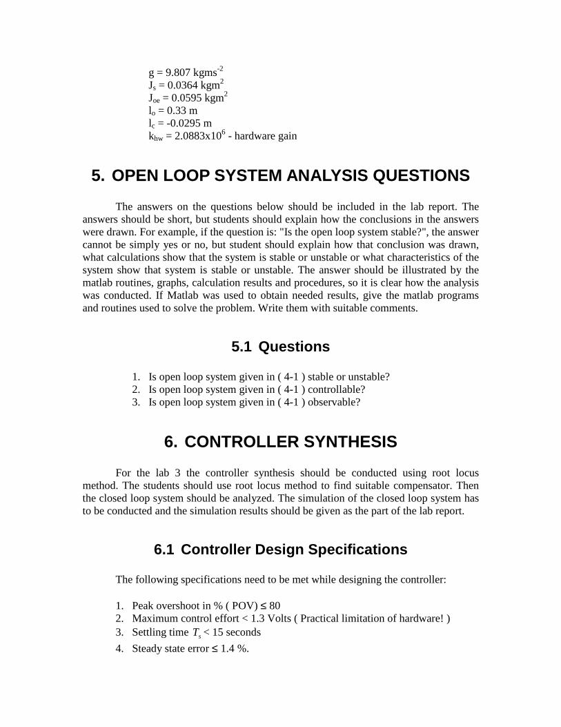
g = 9.807 kgms-2 Js = 0.0364 kgm2 Joe = 0.0595 kgm2

lo = 0.33 m lc = -0.0295 m khw = 2.0883x106 - hardware gain

5. OPEN LOOP SYSTEM ANALYSIS QUESTIONS The answers on the questions below should be included in the lab report. The

answers should be short, but students should explain how the conclusions in the answers were drawn. For example, if the question is: "Is the open loop system stable?", the answer cannot be simply yes or no, but student should explain how that conclusion was drawn, what calculations show that the system is stable or unstable or what characteristics of the system show that system is stable or unstable. The answer should be illustrated by the matlab routines, graphs, calculation results and procedures, so it is clear how the analysis was conducted. If Matlab was used to obtain needed results, give the matlab programs and routines used to solve the problem. Write them with suitable comments.

5.1 Questions

1. Is open loop system given in ( 4-1 ) stable or unstable? 2. Is open loop system given in ( 4-1 ) controllable? 3. Is open loop system given in ( 4-1 ) observable?

6. CONTROLLER SYNTHESIS For the lab 3 the controller synthesis should be conducted using root locus

method. The students should use root locus method to find suitable compensator. Then the closed loop system should be analyzed. The simulation of the closed loop system has to be conducted and the simulation results should be given as the part of the lab report.

6.1 Controller Design Specifications The following specifications need to be met while designing the controller: 1. Peak overshoot in % ( POV) ≤ 80 2. Maximum control effort < 1.3 Volts ( Practical limitation of hardware! ) 3. Settling time sT < 15 seconds

4. Steady state error ≤ 1.4 %.

6.2 Questions The questions after the question No 1 should be answered only if the answer for

the question 1 is "yes".

1. Is it possible to design the controller for the system given in ( 4-1 )? 2. Use root locus method to design the controller (compensator). Describe

the design procedure. Be sure that the compensator can be realized (no zeros can be used that are not compensated by the poles). In the report write the compensator in it’s mathematical form.

3. Plot the root locus of the closed loop system. How it can be seen that the closed loop system is stable from the root locus plot?

4. Include the closed loop poles and zeros in the report. Can you draw some conclusions on the system response based on the closed loop poles and zeros?

5. Simulate the closed loop system step response. The input step value should be –500 counts. Plot the step response.

6. Analyze the step response. Give the peak value, settling time and natural frequency of the system. Compare the response with the poles and zeros of the system. Are the results of the simulation as expected? Explain how you have obtained the peak value, settling time and natural frequency. Illustrate with figures if necessary.

7. Plot the error, the rod displacement and the control output for the time span t = 15 s.

7. IMPLEMENTATION OF THE CONTROLLER ON THE REAL TIME HARDWARE

The controller obtained should be implemented on the real time hardware. Lab

setup is consisted of ECP model 505 (inverted pendulum) with the Mini PMAC V1.16D card inside PC. The software used for the real time control is QRTS ECP extension form Matlab R12/Simulink 4. It works under Real Time Workshop and Real Time Windows Target for Simulink 4. The Simulink block diagram is shown in Fig. 2.

Fig. 2: Simulink block diagram for running QRTS ECP extension

Students should use their own compensator (block "comp"). The reference value

should be step of –500 counts at t = 0 s and then step from –500 counts to 0 at t = 15 s. The whole experiment should be conducted for the time span t = 30 s. The reference value time plot is shown in Fig. 3.

� � � � � � � � � � � �� � � �� � � �� � � �� � � �� � � �� � � �� � � �� � � �� � � �� � ��

� �� �������� !�" �#!�$ %&

' ( ) *

Fig. 3: Reference value for the experiment

Mini Pmac Server Module (green block) is the hardware interface module used to

run the hardware. By double click on that module you can change number of encoders that will be read from the hardware setup.

Safety modules (red blocks) are used to protect the hardware from the possible damage due to controller improper operation.

The controller designed as a part of the solution for the section 6 should be in the place of the block "controller" in Fig. 2

7.1 Questions

1. Implement you own compensator and run the experiment with the given reference value for 30 s.

2. Plot the rod displacement, reference value, control effort and the control error.

3. What can you conclude from the experiment results? Are there significant nonlinearities present in the real system?

4. Compare the obtained plots from the experiment with the theoretical analysis results form section 5. Are there significant differences? If so, what could cause them? What you could say about the model given in section 5 based on the comparison of the experiment and simulation results?

8. TABLE OF FIGURES

Fig. 1: Inverted pendulum apparatus...................................................................................4 Fig. 2: Simulink block diagram for running QRTS ECP extension....................................7 Fig. 3: Reference value for the experiment .........................................................................7