EE360: Multiuser Wireless Systems and Networks

Lecture 3 OutlineAnnouncements

Makeup lecture Feb 2, 5-6:15. Presentation schedule will be sent out later

today, presentations will start 1/30. Next lecture: Random/Multiple Access, SS, MUD

Capacity of Broadcast ISI ChannelsCapacity of MAC Channels

In AWGN In Fading and ISI

Duality between the MAC and the BC

Capacity of MIMO Multiuser Channels

Review of Last Lecture

Channel capacity region of broadcast channels Capacity in AWGN

Use superposition coding and optimal power allocation Capacity in fading

Ergodic capacity: optimally allocate resources over timeOutage capacity: maintain fixed rates in all statesMinimum rate capacity: fixed min. rate in all states, use excess rsources to optimize average rate above min.

Broadcast: One Transmitter to Many Receivers.

R1

R2R3

x g1(t)x g2(t)

x g3(t)

Broadcast Channels with ISI

ISI introduces memory into the channel

The optimal coding strategy decomposes the channel into parallel broadcast channelsSuperposition coding is applied to each

subchannel.

Power must be optimized across subchannels and between users in each subchannel.

Broadcast Channel Model

Both H1 and H2 are finite IR filters of length m.

The w1k and w2k are correlated noise samples. For 1<k<n, we call this channel the n-block

discrete Gaussian broadcast channel (n-DGBC). The channel capacity region is C=(R1,R2).

w1k

H1(f)

H2(f)w2k

xk

y h x wk ii

m

kk i1 11

1

y h x wk ii

m

kk i2 21

2

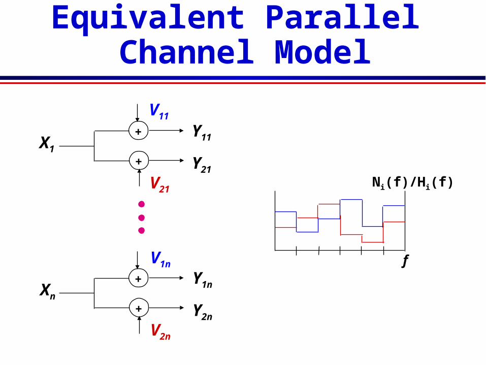
Equivalent Parallel Channel Model

+

+X1

V11

V21

Y11

Y21

+

+Xn

V1n

V2n

Y1n

Y2n

Ni(f)/Hi(f)

f

Channel Decomposition

Via a DFT, the BC with ISI approximately decomposes into n parallel AWGN degraded broadcast channels.

As n goes to infinity, this parallel model becomes exact

The capacity region of parallel degraded broadcast channels was obtained by El-Gamal (1980)

Optimal power allocation obtained by Hughes-Hartogs(’75).

The power constraint on the original channel is converted by Parseval’s theorem to on the equivalent channel.

E x nPii

n

[ ]2

0

1

E X n Pii

n

[( ) ]

0

12 2

Capacity Region of Parallel Set

Achievable Rates (no common information)

Capacity Region For 0< find {j}, {Pj} to maximize R1+R2+ Pj. Let (R1

*,R2*)n, denote the corresponding rate pair.

Cn={(R1*,R2

*)n, : 0< }, C=liminfn Cn .

1n

PnP

P

P

PR

P

PPR

jj

j j

jj

j jjj

jj

j jjj

jj

j j

jj

jjjj

jjjj

2

: 2: 22

: 1: 11

,10

,)1(

1log5.)1(

1log5.

,)1(

1log5.1log5.

2121

2121

R1

R2

Limiting Capacity Region

PdffPf

N

fHfPf

fHNfPf

fPfR

P

P

N

fHfPfR

fHfHffHfHf

fHfHf jjj

jj

fHfHf

)(,1)(0

,5.

|)(|)())(1(1log5.

|)(|/5.)()(

)())(1(1log5.

,)1(

1log5.5.

|)(|)()(1log5.

)()(: 0

22

)()(:2

202

)()(: 1)()(: 0

21

1

2121

2121

Optimal Power Allocation:

Two Level Water Filling

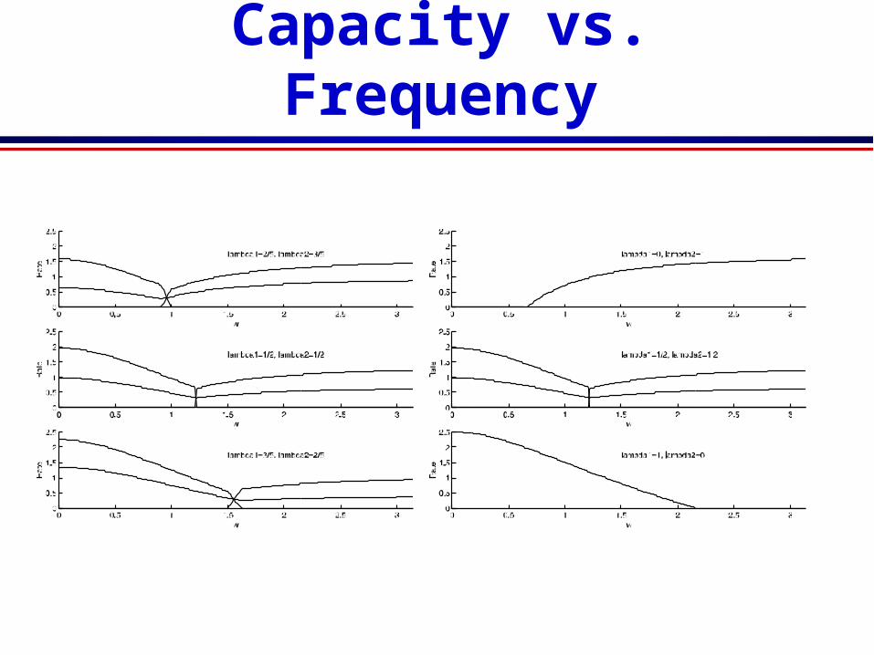
Capacity vs. Frequency

Capacity Region

Multiple Access Channel

Multiple transmitters Transmitter i sends signal Xi with power Pi

Common receiver with AWGN of power

N0B

Received signal:NXYM

ii

1

X1

X2 X3

MAC Capacity Region

Closed convex hull of all (R1,…,RM) s.t.

For all subsets of users, rate sum equals that of 1 superuser with sum of powers from all users

Power Allocation and Decoding Order Each user has its own power (no power alloc.) Decoding order depends on desired rate point

},...,1{,/1log 0 MSBNPBRSi

iSi

i

Two-User RegionSuperposition codingw/ interference canc.

SC w/ IC and timesharing or rate splitting

Frequency division

Time division

C1

C2

Ĉ1

Ĉ2

2,1,1log0

i

BN

PBC i

i

,1logˆ,1logˆ10

22

20

11

PBN

PBC

PBN

PBC

SC w/out IC

Fading and ISI

MAC capacity under fading and ISI determined using similar techniques as for the BC

In fading, can define ergodic, outage, and minimum rate capacity similar as in BC caseErgodic capacity obtained based on AWGN MAC

given fixed fading, averaged over fading statisticsOutage can be declared as common, or per user

MAC capacity with ISI obtained by converting to equivalent parallel MAC channels over frequency

Characteristics

Corner points achieved by 1 user operating at his maximum rate Other users operate at rate which can be

decoded perfectly and subtracted out (IC)

Time sharing connects corner points Can also achieve this line via rate splitting,

where one user “splits” into virtual users

FD has rate RiBilog[1+Pi/(N0B)]

TD is straight line connecting end points With variable power, it is the same as FD

CD without IC is box

Fading MAC Channels

Noise is AWGN with variance 2. Joint fading state (known at TX and

RX):

x

)(1 nh

x

)(nhM

x

)(nz)(1 nx

)(nxM

)(ny

)( 1P

)( MP

)()()()(1

nznxnhny i

M

ii

h=(h1(n),…,hM(n))

Capacity Region*

Rate allocation R(h) RM Power allocation P(h) RM

Subject to power constraints: Eh[P(h)]P

Boundary points: R* RM s.t. [R(h),P(h)] solves

},...,1{,1log5...max2

MSPh

RtsSi

Si iii

PR

with Eh[Ri(h)]=Ri*

*Tse/Hanly, 1996

Unique Decoding Order*

For every boundary point R*:There is a unique decoding order that is the

same for every fading stateDecoding order is reverse order of the priorities

Implications:Given decoding order, only need to optimally

allocate power across fading statesWithout unique decoding order, utility

functions used to get optimal rate and power allocation

*S. Vishwanath

1,...1,:...1 MMM order Decoding

Characteristics of Optimum Power

Allocation

A user’s power in a given state depends only on: His channel (hik) Channels of users decoded just before (hik-1) and just

after (hik+1) Power increases with hik and decreases with hik-1 and

hik+1 Power allocation is a modified waterfilling, modified

to interference from active users just before and just after

User decoded first waterfills to SIR for all active users

Transmission Regions

The region where no users transmit is a hypercube Each user has a unique cutoff below which he does

not transmit

For highest priority user, always transmits above some h1

*

The lowest priority user, even with a great channel, doesn’t transmit if some other user has a relatively good channel

h1

h2

P1>0,P2=0

P1>0,P2>0P1=0,P2>0

P1=0P2=0

1>2

Two User Example

Power allocation for 1>2

0)(,1

)/(

0)(,1

0

)(

21

11

12121

21

21

11

11

1

1

11

1

hPhhhh

hPhh

h

hP

2

2

11

2

2

11

2

2

2

2

11

2

2

)(1

)(1)(1

0)(

hPh

h

h

hPhhPh

h

hP

Ergodic Capacity Summary

Rate region boundary achieved via optimal allocation of power and decoding order

For any boundary point, decoding order is the same for all states Only depends on user priorities

Optimal power allocation obtained via Lagrangian optimization Only depends on users decoded just before and

after Power allocation is a modified waterfilling Transmission regions have cutoff and critical values

MAC Channel with ISI*

Use DFT Decomposition Obtain parallel MAC channels Must determine each user’s power

allocation across subchannels and decoding order

Capacity region no longer a pentagon

X1

X2

H1(f)

H2(f)

*Cheng and Verdu, IT’93

Optimal Power Allocation

Capacity region boundary: maximize

1R1+2R2

Decoding order based on priorities and channels

Power allocation is a two-level water fillingTotal power of both users is scaled water level In non-overlapping region, best user gets all

power (FD)With overlap, power allocation and decoding

order based on s and user channels.

b1/|H1(f)|2+

b2/|H2(f)|2+

1

Differences:Shared vs. individual power constraintsNear-far effect in MAC

Similarities:Optimal BC “superposition” coding is also

optimal for MAC (sum of Gaussian codewords)

Both decoders exploit successive decoding and interference cancellation

Comparison of MAC and BC

P

P1

P2

MAC-BC Capacity Regions

MAC capacity region known for many casesConvex optimization problem

BC capacity region typically only known for (parallel) degraded channelsFormulas often not convex

Can we find a connection between the BC and MAC capacity regions?Duality

Dual Broadcast and MAC Channels

x

)(1 nh

x

)(nhM

+

)(1 nz

)(1 nx

)(nxM

)(1 ny)( 1P

)( MP

x

)(1 nh

x

)(nhM

+

)(nzM

)(nyM

+

)(nz

)(ny)(nx)(P

Gaussian BC and MAC with same channel gains and same noise power at each receiver

Broadcast Channel (BC)Multiple-Access Channel (MAC)

The BC from the MAC

Blue = BCRed = MAC

21 hh

P1=1, P2=1

P1=1.5, P2=0.5

P1=0.5, P2=1.5

),;(),;,( 21212121 hhPPChhPPC BCMAC

MAC with sum-power constraint

PP

MACBC hhPPPChhPC

10

211121 ),;,(),;(

Sum-Power MAC

MAC with sum power constraintPower pooled between MAC

transmittersNo transmitter coordination

P

P

MAC BCSame capacity region!

),;(),;,(),;( 210

211121

1

hhPChhPPPChhPC SumMAC

PPMACBC

BC to MAC: Channel Scaling

Scale channel gain by , power by 1/ MAC capacity region unaffected by scaling Scaled MAC capacity region is a subset of the

scaled BC capacity region for any MAC region inside scaled BC region for

anyscaling

1h

1P

2P2h

+

+

21 PP

1h

2h+

MAC

BC

The BC from the MAC

0

2121

2121 ),;(),;,(

hhPP

ChhPPC BCMAC

Blue = Scaled BCRed = MAC

1

2

h

h

0

BC in terms of MAC

MAC in terms of BC

PP

MACBC hhPPPChhPC

10

211121 ),;,(),;(

0

2121

2121 ),;(),;,(

hhPP

ChhPPC BCMAC

Duality: Constant AWGN Channels

What is the relationship betweenthe optimal transmission strategies?

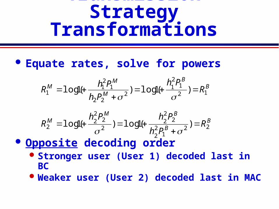
Equate rates, solve for powers

Opposite decoding order Stronger user (User 1) decoded last in BCWeaker user (User 2) decoded last in MAC

Transmission Strategy

Transformations

BB

BMM

BB

M

MM

RPh

PhPhR

RPh

Ph

PhR

221

22

222

2

222

2

12

121

222

121

1

)1log()1log(

)1log()1log(

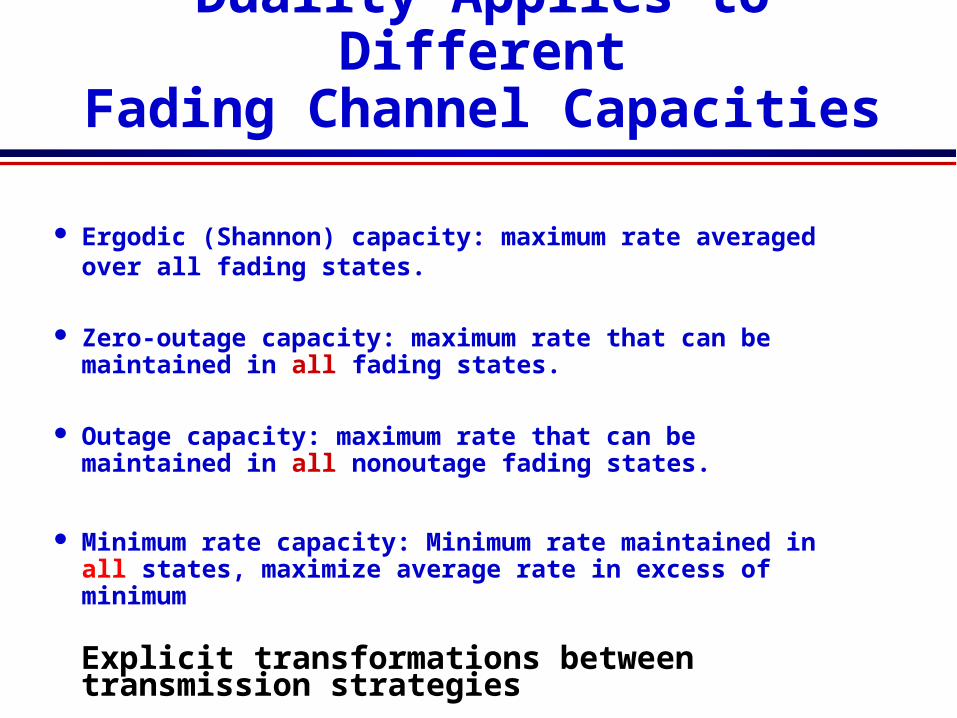
Duality Applies to Different

Fading Channel Capacities

Ergodic (Shannon) capacity: maximum rate averaged over all fading states.

Zero-outage capacity: maximum rate that can be maintained in all fading states.

Outage capacity: maximum rate that can be maintained in all nonoutage fading states.

Minimum rate capacity: Minimum rate maintained in all states, maximize average rate in excess of minimum

Explicit transformations between transmission strategies

Duality: Minimum Rate Capacity

BC region known MAC region can only be obtained by duality

Blue = Scaled BCRed = MAC

MAC in terms of BC

What other capacity regions can be obtained by duality?Broadcast MIMO

Channels

Broadcast MIMO Channel

111 n x H y 1H

x

1n

222 n x H y 2H

2n

t1 TX antennasr11, r21 RX antennas

)1 t(r

)2 t(r

)IN(0,~n)IN(0,~n21 r2r1

Non-degraded broadcast channel

Perfect CSI at TX and RX

Dirty Paper Coding (Costa’83)

Dirty Paper Coding

Clean Channel Dirty Channel

Dirty Paper

Coding

Basic premiseIf the interference is known, channel

capacity same as if there is no interferenceAccomplished by cleverly distributing the

writing (codewords) and coloring their inkDecoder must know how to read these

codewords

Modulo Encoding/Decoding

Received signal Y=X+S, -1X1 S known to transmitter, not receiver

Modulo operation removes the interference effects Set X so that Y[-1,1]=desired message (e.g. 0.5) Receiver demodulates modulo [-1,1]

-1 +3 +5+1-3

…-5 0

S

-1 +10

-1 +10

X

+7-7

…

Capacity Results Non-degraded broadcast channel

Receivers not necessarily “better” or “worse” due to multiple transmit/receive antennas

Capacity region for general case unknown

Pioneering work by Caire/Shamai (Allerton’00): Two TX antennas/two RXs (1 antenna each) Dirty paper coding/lattice precoding

(achievable rate) Computationally very complex

MIMO version of the Sato upper bound Upper bound is achievable: capacity known!

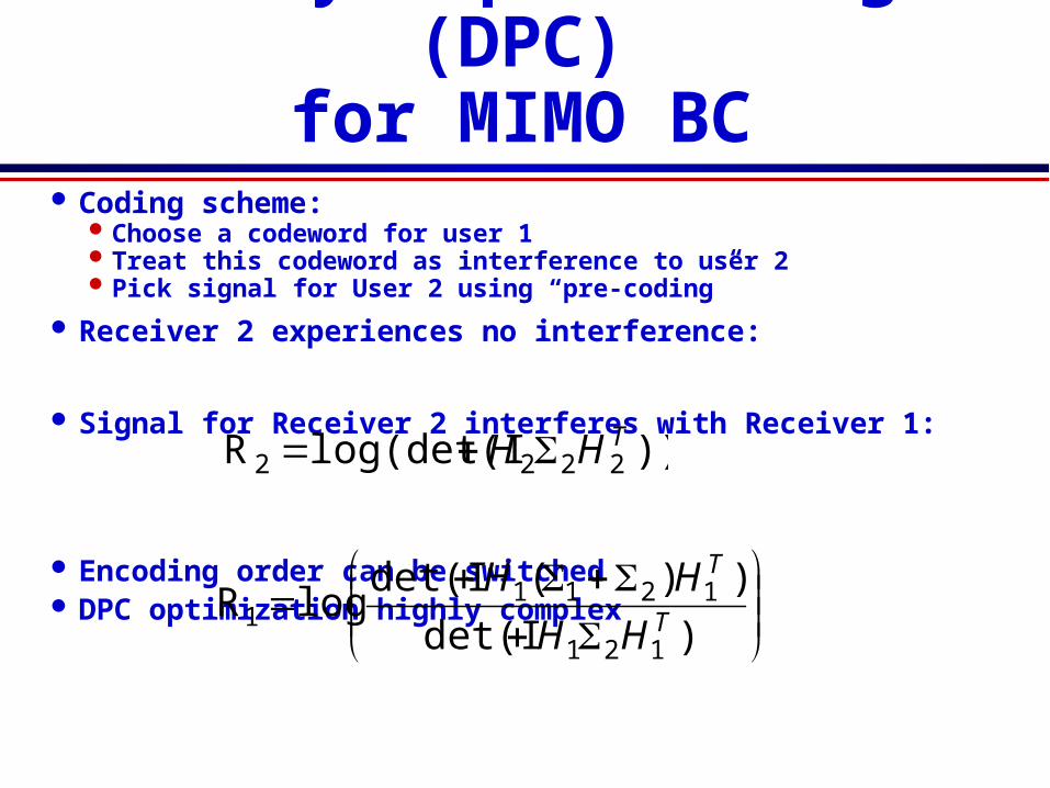
Dirty-Paper Coding (DPC)

for MIMO BC Coding scheme:

Choose a codeword for user 1Treat this codeword as interference to user 2Pick signal for User 2 using “pre-coding”

Receiver 2 experiences no interference:

Signal for Receiver 2 interferes with Receiver 1:

Encoding order can be switched DPC optimization highly complex

)) log(det(I R 2222THH

) det(I

))( det(Ilog R

121

12111 T

T

HH

HH

Does DPC achieve capacity?

DPC yields MIMO BC achievable region.We call this the dirty-paper region

Is this region the capacity region?

We use duality, dirty paper coding, and Sato’s upper bound to address this question

First we need MIMO MAC Capacity

MIMO MAC Capacity MIMO MAC follows from MAC capacity formula

Basic idea same as single user case Pick some subset of users The sum of those user rates equals the capacity as if

the users pooled their power

Power Allocation and Decoding Order Each user has its own power (no power alloc.) Decoding order depends on desired rate point

Sk Sk

HkkkkkkMAC HQHIRRRPPC ,detlog:),...,(),...,( 211

},...,1{ KS

MIMO MAC with sum power

MAC with sum power: Transmitters code independentlyShare power

Theorem: Dirty-paper BC region equals the dual sum-power MAC region

PP

MACSumMAC PPPCPC

10

11 ),()(

)()( PCPC SumMAC

DPCBC

P

Transformations: MAC to BC

Show any rate achievable in sum-power MAC also achievable with DPC for BC:

A sum-power MAC strategy for point (R1,…RN) has a given input covariance matrix and encoding order

We find the corresponding PSD covariance matrix and encoding order to achieve (R1,…,RN) with DPC on BC

The rank-preserving transform “flips the effective channel” and reverses the order

Side result: beamforming is optimal for BC with 1 Rx antenna at each mobile

)()( PCPC SumMAC

DPCBC

DPC BC Sum MAC

Transformations: BC to MAC

Show any rate achievable with DPC in BC also achievable in sum-power MAC:

We find transformation between optimal DPC strategy and optimal sum-power MAC strategy

“Flip the effective channel” and reverse order

)()( PCPC SumMAC

DPCBC

DPC BC Sum MAC

Computing the Capacity Region

Hard to compute DPC region (Caire/Shamai’00)

“Easy” to compute the MIMO MAC capacity region Obtain DPC region by solving for sum-

power MAC and applying the theorem Fast iterative algorithms have been

developed Greatly simplifies calculation of the DPC

region and the associated transmit strategy

)()( PCPC SumMAC

DPCBC

Based on receiver cooperation

BC sum rate capacity Cooperative capacity

Sato Upper Bound on the

BC Capacity Region

+

+

1H

2H

1n

2n

1y

2y

x

|HHΣI|log2

1maxH)(P, T

xsumrateBC

x

C

Joint receiver

The Sato Bound for MIMO BC

Introduce noise correlation between receivers BC capacity region unaffected

Only depends on noise marginals

Tight Bound (Caire/Shamai’00) Cooperative capacity with worst-case noise correlation

Explicit formula for worst-case noise covariance By Lagrangian duality, cooperative BC region equals

the sum-rate capacity region of MIMO MAC

|ΣHHΣΣI|log2

1maxinfH)(P, 1/2

zT

x1/2

zsumrateBC

xz

C

MIMO BC Capacity Bounds

Sato Upper Bound

Single User Capacity BoundsDirty Paper Achievable Region

BC Sum Rate Point

Does the DPC region equal the capacity region?

Full Capacity Region DPC gives us an achievable region

Sato bound only touches at sum-rate point

Bergman’s entropy power inequality is not a tight upper bound for nondegraded broadcast channel

A tighter bound was needed to prove DPC optimal It had been shown that if Gaussian codes optimal, DPC

was optimal, but proving Gaussian optimality was open.

Breakthrough by Weingarten, Steinberg and Shamai Introduce notion of enhanced channel, applied Bergman’s

converse to it to prove DPC optimal for MIMO BC.

Enhanced Channel Idea

The aligned and degraded BC (AMBC) Unity matrix channel, noise innovations process Limit of AMBC capacity equals that of MIMO BC Eigenvalues of some noise covariances go to infinity Total power mapped to covariance matrix constraint

Capacity region of AMBC achieved by Gaussian superposition coding and successive decoding Uses entropy power inequality on enhanced channel Enhanced channel has less noise variance than original Can show that a power allocation exists whereby the

enhanced channel rate is inside original capacity region

By appropriate power alignment, capacities equal

Illustration

Enhanced

Original

Main Points Shannon capacity gives fundamental data rate limits for

multiuser wireless channels

Fading multiuser channels optimize at each channel instance for maximum average rate

Outage capacity has higher (fixed) rates than with no outage.

OFDM is near optimal for broadcast channels with ISI

Duality connects BC and MAC channels Used to obtain capacity of one from the other

Capacity of broadcast MIMO channel obtained using duality and the notion of an enhanced channel