ee4.07codingtheory - ee.ic.ac.uk · w.dai(ic) ee4.07codingtheory syllabus 2017 page0-1. contents...
TRANSCRIPT
EE4.07 Coding Theory
W. Dai
Imperial College London (IC)
2017
W. Dai (IC) EE4.07 Coding Theory 2017 page 0-1
Syllabus
Instructor: Dr. Wei DaiLectures:I Monday 16:00-17:00, 509B (Wks 2-11, 09/10/2017 - 11/12/2017)
I Wednesday 11:00-12:00 (Wks 2-11, 11/10/2017 - 13/12/2017)
I 407B, Wk 3, 18/10/2017I 509A, Wks 2,4-11
I ?? Wednesday 11:00-13:00 ??Assessment: Exam (75%) and coursework (25%)Textbook: No textbook is required. You can rely on lecture notes.References:I “Introduction to coding theory” Ron M. RothI “Coding Theory: a First Course,” S. Lin and C. XingI “Codes: An Introduction to Information Communication and
Cryptography,” N. L. Biggs
W. Dai (IC) EE4.07 Coding Theory Syllabus 2017 page 0-1
Contents
1. Mathematical foundations: finite fields2. Cryptography
I Password management: store, exchange, and shareI Public key cryptographyI Digital signature
3. Error correcting codesI Linear block codesI Hamming codesI Reed-Solomon codes and decoding
4. Modern codesI Brief introduction to information theoryI Low-density parity check (LDPC) codesI Polar codes
W. Dai (IC) EE4.07 Coding Theory Syllabus 2017 page 0-2

Section 1Finite Fields
I Basic factsI Euclidean algorithmI Unique factorisation theorem
I Finite fields: definition and constructionI Finite fields: general propertiesI Primitive elementsI Polynomial factorisation and minimal polynomials
For basic number theory, the best reference is Wikipedia.For contents relevant to finite fields, refer to Lin&Xing’s book, Chapter 3.
W. Dai (IC) EE4.07 Coding Theory Finite Fields 2017 page 1-1

Two Facts for Coding Theory
Euclidean geometry: all theorems are derived from a small number ofaxioms.
This course: mostly relies on two facts.I A polynomial of degree n has at most n roots.I Every positive integer n > 1 can be uniquely represented as a product
of prime numbers. (will be proved.)
W. Dai (IC) EE4.07 Coding Theory Finite Fields 2017 page 1-2

Greatest Common Divisor (GCD)
How to find the gcd for 0 < b < a?
gcd (5, 13) = 1. (Easy!)gcd (20, 36) = 4. (OK)But gcd (654, 2406) =?
W. Dai (IC) EE4.07 Coding Theory Finite Fields Euclidean algorithm 2017 page 1-3
The Euclidean Algorithm
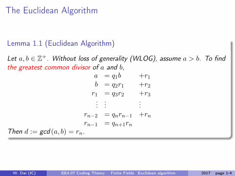
Lemma 1.1 (Euclidean Algorithm)
Let a, b ∈ Z+. Without loss of generality (WLOG), assume a > b. To findthe greatest common divisor of a and b,
a = q1b +r1b = q2r1 +r2r1 = q3r2 +r3...
......
rn−2 = qnrn−1 +rnrn−1 = qn+1rn
Then d := gcd (a, b) = rn.
W. Dai (IC) EE4.07 Coding Theory Finite Fields Euclidean algorithm 2017 page 1-4

The Euclidean Algorithm: An Example
Example 1.2
gcd (654, 2406) =?:2406 = 3× 654 +444654 = 1× 444 +210444 = 2× 210 +24210 = 8× 24 +1824 = 1× 18 +618 = 3× 6
gcd (654, 2406) = 6.
W. Dai (IC) EE4.07 Coding Theory Finite Fields Euclidean algorithm 2017 page 1-5

The Euclidean Algorithm: Theory
Theorem 1.3For 0 < b < a, define r = a mod b 6= 0. Then gcd (a, b) = gcd (b, r).
Proof: Let a = bq + r where 1 ≤ r < b.Let d1 = gcd (a, b) and d2 = gcd (b, r). Want to show d1 = d2.
d1|a and d1|b ⇒ d1| (a− bq) ⇒ d1|rd2 = gcd (b, r)
}⇒ d1 ≤ d2.
d2|b and d2|r ⇒ d2| (bq + r) ⇒ d2|ad1 = gcd (a, b)
}⇒ d2 ≤ d1.
Therefore, d1 = d2. ♦
Corollary 1.4 (Validation of Euclidean Alg.)In the Euclidean algorithm,gcd (a, b) = gcd (b, r1) = · · · = gcd (rn−1, rn) = rn.
W. Dai (IC) EE4.07 Coding Theory Finite Fields Euclidean algorithm 2017 page 1-6

Bézout’s IdentityLemma 1.5 (Bézout’s Identity or Bézout’s Lemma)
Given positive integers a and b, let d = gcd (a, b). Then d can be writtenas an integer linear combination of a and b, i.e., ∃x, y ∈ Z s.t.d = gcd (a, b) = xa+ yb.
Proof:
rn = −qnrn−1 + rn−2= −qn (−qn−1rn−2 + rn−3) + rn−2= (1 + qnqn−1) rn−2 − qnrn−3= · · · = xa+ yb.
♦
Example 1.6 (gcd (13, 5) = 1)
Euclidean Alg. Bézout’s Identity13 = 2 · 5 + 35 = 1 · 3 + 23 = 1 · 2 + 12 = 2 · 1
1 = 3− 2= 3− (5− 3) = 2 · 3− 5= 2 · (13− 2 · 5)− 5 = 2 · 13−5 · 5
W. Dai (IC) EE4.07 Coding Theory Finite Fields Euclidean algorithm 2017 page 1-7

GCD of Polynomials
The GCD of two polynomials is a polynomial, of the highest degree, thatdivides both original polynomials.
In this course, the convention is that the leading coefficient is 1.
Example 1.7
gcd(x2 − 1, 2x− 2
)={x− 1, 2x− 2, 1
2x−12 , 10
6x− 106}.
By convention, gcd(x2 − 1, 2x− 2
)= x− 1.
W. Dai (IC) EE4.07 Coding Theory Finite Fields Euclidean algorithm 2017 page 1-8
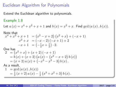
Euclidean Algorithm for Polynomials
Extend the Euclidean algorithm to polynomials.
Example 1.8Let a (x) = x4 + x2 + x+ 1 and b (x) = x2 + x. Find gcd (a (x) , b (x)).
Note thatx4 + x2 + x+ 1 =
(x2 − x+ 2
) (x2 + x
)+ (−x+ 1)
x2 + x = (−x− 2) (−x+ 1) + 2−x+ 1 =
(−1
2x+ 12
)· 2.
One has2 =
(x2 + x
)+ (x+ 2) (−x+ 1)
= b (x) + (x+ 2)(a (x)−
(x2 − x+ 2
)b (x)
)= (x+ 2) a (x) +
(−x3 − x2 − 3
)b (x) .
As a result,1 = gcd (a (x) , b (x))
= 12 (x+ 2) a (x)− 1
2
(x3 + x2 + 3
)b (x) .
W. Dai (IC) EE4.07 Coding Theory Finite Fields Euclidean algorithm 2017 page 1-9
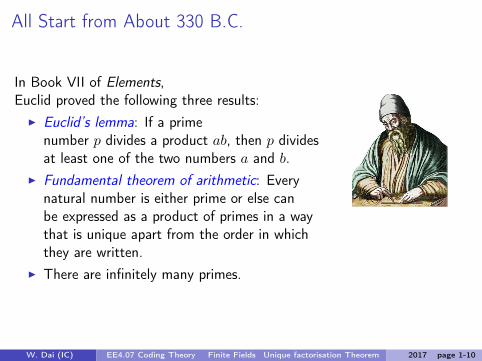
All Start from About 330 B.C.
In Book VII of Elements,Euclid proved the following three results:I Euclid’s lemma: If a prime
number p divides a product ab, then p dividesat least one of the two numbers a and b.
I Fundamental theorem of arithmetic: Everynatural number is either prime or else canbe expressed as a product of primes in a waythat is unique apart from the order in whichthey are written.
I There are infinitely many primes.
W. Dai (IC) EE4.07 Coding Theory Finite Fields Unique factorisation Theorem 2017 page 1-10
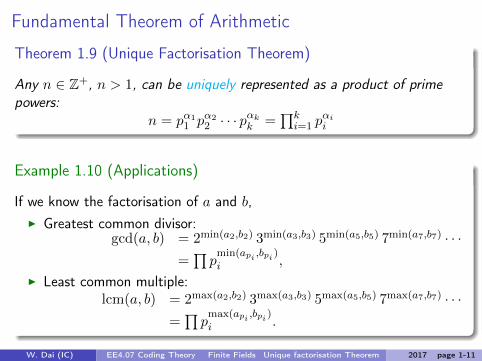
Fundamental Theorem of Arithmetic
Theorem 1.9 (Unique Factorisation Theorem)
Any n ∈ Z+, n > 1, can be uniquely represented as a product of primepowers:
n = pα11 pα2
2 · · · pαkk =
∏ki=1 p
αii
Example 1.10 (Applications)
If we know the factorisation of a and b,I Greatest common divisor:
gcd(a, b) = 2min(a2,b2) 3min(a3,b3) 5min(a5,b5) 7min(a7,b7) · · ·=∏pmin(api ,bpi )i ,
I Least common multiple:lcm(a, b) = 2max(a2,b2) 3max(a3,b3) 5max(a5,b5) 7max(a7,b7) · · ·
=∏pmax(api ,bpi )i .
W. Dai (IC) EE4.07 Coding Theory Finite Fields Unique factorisation Theorem 2017 page 1-11

Some Examples
Example 1.11
4 = 22.6 = 2 · 3. ⇒ gcd (4, 6) = 21 · 30 = 2.
lcm (4, 6) = 22 · 31 = 12.
4 = 22.9 = 32.
⇒ gcd (4, 9) = 20 · 30 = 1.lcm (4, 9) = 22 · 32 = 36.
654 = 2 · 3 · 109.2406 = 2 · 3 · 401. ⇒ gcd (654, 2406) = 6.
lcm (654, 2406) = 262254.
W. Dai (IC) EE4.07 Coding Theory Finite Fields Unique factorisation Theorem 2017 page 1-12
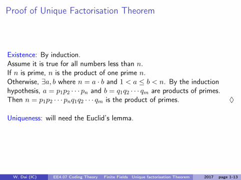
Proof of Unique Factorisation Theorem
Existence: By induction.Assume it is true for all numbers less than n.If n is prime, n is the product of one prime n.Otherwise, ∃a, b where n = a · b and 1 < a ≤ b < n. By the inductionhypothesis, a = p1p2 · · · pn and b = q1q2 · · · qm are products of primes.Then n = p1p2 · · · pnq1q2 · · · qm is the product of primes. ♦
Uniqueness: will need the Euclid’s lemma.
W. Dai (IC) EE4.07 Coding Theory Finite Fields Unique factorisation Theorem 2017 page 1-13
Euclid’s Lemma
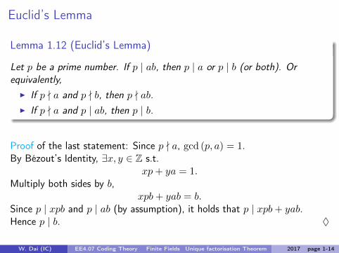
Lemma 1.12 (Euclid’s Lemma)
Let p be a prime number. If p | ab, then p | a or p | b (or both). Orequivalently,I If p - a and p - b, then p - ab.I If p - a and p | ab, then p | b.
Proof of the last statement: Since p - a, gcd (p, a) = 1.By Bézout’s Identity, ∃x, y ∈ Z s.t.
xp+ ya = 1.Multiply both sides by b,
xpb+ yab = b.Since p | xpb and p | ab (by assumption), it holds that p | xpb+ yab.Hence p | b. ♦
W. Dai (IC) EE4.07 Coding Theory Finite Fields Unique factorisation Theorem 2017 page 1-14
Proof of Unique Factorisation Theorem (Uniqueness)
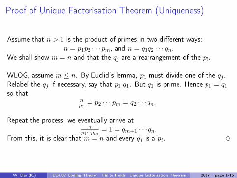
Assume that n > 1 is the product of primes in two different ways:n = p1p2 · · · pm, and n = q1q2 · · · qn.
We shall show m = n and that the qj are a rearrangement of the pi.
WLOG, assume m ≤ n. By Euclid’s lemma, p1 must divide one of the qj .Relabel the qj if necessary, say that p1|q1. But q1 is prime. Hence p1 = q1so that
np1
= p2 · · · pm = q2 · · · qn.
Repeat the process, we eventually arrive atn
p1···pm = 1 = qm+1 · · · qn.From this, it is clear that m = n and every qj is a pi. ♦
W. Dai (IC) EE4.07 Coding Theory Finite Fields Unique factorisation Theorem 2017 page 1-15

Gauss’s Clock Arithmetic
In 1801when Gauss was 24, he wrote a book DisquisitionesArithmeticae, one of the most influential mathematicsbooks ever. One of the topics is finite arithmetic.
Modulusof arithmetic: Count hours as 0, 1, 2, · · · , 11. Then
2 + 3 ≡ 5 (mod 12) , 7 + 6 ≡ 1 (mod 12) ,
where ≡ stands for congruence. Similarly,
5× 5 ≡ 1 (mod 12) , 11× 5 ≡ 7 (mod 12) .
It is clear that 1/5 ≡ 5 (mod 12) and 7/5 ≡ 11 (mod 12).However, 5/6 (mod 12) is not defined.
W. Dai (IC) EE4.07 Coding Theory Finite Fields Definition 2017 page 1-16

Fields: Definition
Definition 1.13 (Field)A field F is a nonempty set of elements with two operations, called addition(+) and multiplication (·).I F is closed under + and ·, i.e., a+ b and a · b are in F.
I Commutative: a+ b = b+ aI Associative: a+ (b+ c) = (a+ b) + cI Distributive a (b+ c) = ab+ ac
I Exists two distinct identity 0 and 1 (additive and multiplicativeidentities, respectively)
I a+ 0 = a, ∀a ∈ FI a · 1 = a and a · 0 = 0, ∀a ∈ FI Additive inverse: ∀a ∈ F, ∃ (−a) ∈ F, s.t. a+ (−a) = 0.I Multiplicative inverse: ∀a ∈ F\ {0}, ∃a−1 ∈ F, s.t. a · a−1 = 1.
Example: R, Q, Z7 are fields, Z is not.
W. Dai (IC) EE4.07 Coding Theory Finite Fields Definition 2017 page 1-17

Integer Ring
Definition 1.14 (Modulo)The modulo operator finds the remainder of one number divided byanother.Examples: 5 mod 4 = 1, 14 mod 4 = 2.
Definition 1.15 (Integer Ring)I Zm = {0, · · · ,m− 1}: a nonempty set of elements.I “+” operator: + mod mI “·” operator: · mod m.
Example of m = 4:Zm = {0, 1, 2, 3}.1 + 1 = 2 (mod 4); 2 + 3 = 1 (mod 4).3 · 3 = 1 (mod 4); 2 · 2 = 4 = 0 (mod 4).
W. Dai (IC) EE4.07 Coding Theory Finite Fields Definition 2017 page 1-18

Examples: Integer Rings Versus Fields
I Z3 is a field.I −0 = 0, −1 = 2, −2 = 1.I 1−1 = 1, 2−1 = 2.
I Z4 is not a field.I −0 = 0, −1 = 3, −2 = 2, −3 = 1.I 1−1 = 1, @ 2−1, 3−1 = 3.
W. Dai (IC) EE4.07 Coding Theory Finite Fields Definition 2017 page 1-19

When a Multiplicative Inverse Exists
Lemma 1.16 (Existence of the multiplicative inverse)
Let a, n ∈ Z+ with a < n. The multiplicative inverse a−1 (mod n) existsiff gcd (a, n) = 1.
Proof:1. If gcd (a, n) = 1, by Bézout’s identity ∃x, y s.t.
1 = xn+ ya ≡ ya (mod n). Hence y is a−1.2. If a−1 (mod n) exists, want to show that gcd (a, n) = 1.
Suppose not, i.e., d = gcd (a, n) > 1.By assumption that a−1 exists, ∃x = a−1 and y s.t.1 = xa mod n = xa− yn.As d | a and d | n, it follows d | (xa− yn), i.e. d | 1.This contradicts with d > 1. ♦
W. Dai (IC) EE4.07 Coding Theory Finite Fields Definition 2017 page 1-20

Finite Fields of Integers
Theorem 1.17Zm is a field if and only if m is a prime. (Hence notation Fp.)
Proof of the “if” part: m be a prime⇒Zm is a field.∀a ∈ Zm\ {0}, since m is a prime, one has gcd (a,m) = 1.By Lemma 1.16, a−1 exists. ♦
Proof of the “only if” part: Zm is a field ⇒ m is a prime.Suppose m is not a prime. ∃1 < a, b < m s.t. a · b = m.Since a = gcd (a,m) 6= 1, by Lemma 1.16, a−1 does not exist. ♦
W. Dai (IC) EE4.07 Coding Theory Finite Fields Definition 2017 page 1-21

An Alternative Proof
Recall: Zm is a field if and only if m is a prime. (Hence notation Fp.)
Lemma 1.18
Let a, b ∈ Fp. Then ab = 0 implies a = 0 or b = 0.
Proof: Suppose that a 6= 0. Then 0 = a−1 · 0 = a−1 · (a · b) = b. ♦
Alternative proof of the “only if” part:Suppose m is not a prime.∃1 < a, b < m s.t. a · b = m = 0 (mod m). Butfrom Lemma 1.18, either a or b is zero mod m. Contradict with1 < a, b < m. ♦
W. Dai (IC) EE4.07 Coding Theory Finite Fields Definition 2017 page 1-22

Polynomials
Polynomials over a field Fp: f (x) =∑d
i=0 aixi, ai ∈ Fp.
Degree: highest degree of its terms: deg (f) = d if ad 6= 0.Monic polynomials: ad = 1.
Polynomial division:a (x) = q (x) b (x) + r (x) where 0 ≤ deg (r (x)) < deg (b (x)).
Example: Let a (x) = x3 + x+ 1 ∈ F2 [x] and b (x) = x2 + x ∈ F2 [x].Then a (x) = (x+ 1) b (x) + 1.
f (x) ∈ F [x] is irreducible if f (x) = g (x)h (x) , g, h ∈ F [x], implies eitherg or h is a constant (similar to prime numbers).
W. Dai (IC) EE4.07 Coding Theory Finite Fields Definition 2017 page 1-23

Finite Fields: Polynomials
Fp [x]={g (x) =
∑di=0 aix
i : ai ∈ Fp}.
Fp [x] /f (x): Fp [x] with “mod f (x)” algebra.It contains all the polynomials with degree less than deg (f).
Example: f (x) = x2 + x ∈ F2 [x].F2 [x] /f (x) = {0, 1, x, x+ 1}.x · (x+ 1) = x2 + x ≡ 0 mod f (x).
Theorem 1.19Fp [x] /f (x) is a field iff f (x) is irreducible over Fp.
Proof: Same idea as before.
W. Dai (IC) EE4.07 Coding Theory Finite Fields Definition 2017 page 1-24

Some Comments
Examples of Irreducible polynomials and those that are notI x2 + 1 ∈ R [x] is irreducible.I x2 + 1 ∈ F2 [x] is not irreducible (reducible).I x2 + 1 ∈ F3 [x] is irreducible.I x2 + 1 ∈ F5 [x] is not irreducible.
A systematic way to write the elements in a polynomial ringFp [x] /f (x) where d = deg (f (x)).αdx
d + αd−1xd−1 + · · ·+ α1x+ α0, where αi ∈ Fp.
It contains pd many distinct polynomials.
Size of the finite field FqI Fq contains numbers: q = p.I Fq contains polynomials: q = pd where d = deg (f).
W. Dai (IC) EE4.07 Coding Theory Finite Fields Definition 2017 page 1-25

Example Fields Containing Polynomials
Some irreducible polynomials over F2
x, x+ 1, x2 + x+ 1, x3 + x+ 1, x3 + x2 + 1, x4 + x+ 1, · · ·Each of these polynomial generates a finite field.
Example 1.20
F2 [x] /x3 + x+ 1 F2 [x] /x
3 + x2 + 10 0 01 1 1x x xx2 x2 x2
x3 x+ 1 x2 + 1x4 x2 + x x2 + x+ 1x5 x2 + x+ 1 x+ 1x6 x2 + 1 x2 + x
W. Dai (IC) EE4.07 Coding Theory Finite Fields Definition 2017 page 1-26

Another Example
Example 1.21 (An Example of F16)
F2 [x] /x4 + x+ 1 F2 [x] /x
4 + x+ 10 0 x7 x3 + x+ 11 1 x8 x2 + 1x x x9 x3 + xx2 x2 x10 x2 + x+ 1x3 x3 x11 x3 + x2 + xx4 x+ 1 x12 x3 + x2 + x+ 1x5 x2 + x x13 x3 + x2 + 1x6 x3 + x2 x14 x3 + 1
W. Dai (IC) EE4.07 Coding Theory Finite Fields Definition 2017 page 1-27
Useful Exercise
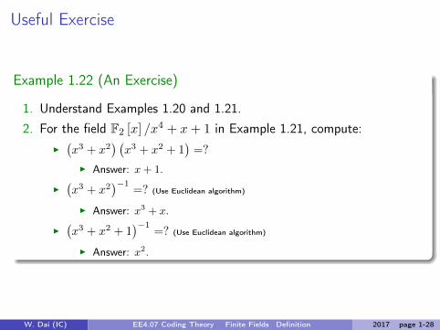
Example 1.22 (An Exercise)
1. Understand Examples 1.20 and 1.21.2. For the field F2 [x] /x
4 + x+ 1 in Example 1.21, compute:I(x3 + x2
) (x3 + x2 + 1
)=?
I Answer: x+ 1.
I(x3 + x2
)−1=? (Use Euclidean algorithm)
I Answer: x3 + x.
I(x3 + x2 + 1
)−1=? (Use Euclidean algorithm)
I Answer: x2.
W. Dai (IC) EE4.07 Coding Theory Finite Fields Definition 2017 page 1-28

Finite Fields: General Properties?
Previously, we saw two ways to construct finite fields.I Fp: p many integers.I Fp [x] /f (x): pdeg(f) many polynomials.
What can we say about the size of a finite field F in general?
W. Dai (IC) EE4.07 Coding Theory Finite Fields Size 2017 page 1-29

Characteristic: Definition
Let F be an arbitrary field.By definition, ∃ a multiplicative identity, denoted by ‘1’.Consider a sequence in Fq: 1, 1 + 1, · · ·
Since |Fq| = q <∞, we will see repetitions.That is, ∃t ∈ Z+ s.t. 1 + · · ·+ 1︸ ︷︷ ︸
t times
= t · 1 = 0.
Remark: To compute 1 + · · · + 1 = t · 1, we have used the algebra defined for this field F.
Definition 1.23The smallest t s.t. t · 1 = 0 is called characteristic of F.
W. Dai (IC) EE4.07 Coding Theory Finite Fields Size 2017 page 1-30

Characteristic: Property
Lemma 1.24The characteristic t is always a prime.
Proof: Otherwise, t · 1 = ab · 1 = 0.1st equation uses normal algebra for integers. 2nd equation uses the algebra for the finite field.
This implies a = 0 or b = 0 (by Lemma 1.18).
Contradict with that t is the smallest.
W. Dai (IC) EE4.07 Coding Theory Finite Fields Size 2017 page 1-31

Finite Fields: Size
Theorem 1.25
All finite fields are of the size pm.
Proof: For any given finite field Fq, let p be its characteristic.
Choose a nonzero element from Fq, say b1.Choose another nonzero element from Fq, say b2, such that b2 and b1 arelinearly independent, i.e.,
λ1b1 + λ2b2 = 0, λ1, λ2 ∈ Fp ⇔ λ1 = λ2 = 0.Consider a maximal set
B = {b1, · · · , bm} ⊂ Fwhich are linearly independent over Fp.
Define the linear span of Bspan (B) = {λ1b1 + · · ·+ λmbm : λi ∈ Fp}.
W. Dai (IC) EE4.07 Coding Theory Finite Fields Size 2017 page 1-32

Finite Fields: Size and Dimension
Proof continued:1. Then |span (B)| = pm ≤ |Fq|.
If(λ(1)1 , · · · , λ(1)
m
)6=(λ(2)1 , · · · , λ(2)
m
), then
∑λ(1)i bi 6=
∑λ(2)i bi.
Suppose not, i.e.,∑λ(1)i bi =
∑λ(2)i bi. Then
∑(λ(1)i − λ
(2)i
)bi = 0 which, by
linear independence of bi’s, implies that λ(1)i = λ
(2)i .
This contradicts the assumption that(λ(1)1 , · · · , λ(1)
m
)6=(λ(2)1 , · · · , λ(2)
m
).
2. It also holds that |span (B)| = |Fq|:Otherwise ∃bm+1 linearly independent of B.This contradicts with the definition of the maximal independent set B.
Hence, for any finite field Fq, q = pm. ♦
B is a basis of Fq.m is the dimension of Fq.
W. Dai (IC) EE4.07 Coding Theory Finite Fields Size 2017 page 1-33

Primitive Elements∀a ∈ F, consider the sequence a, a2, a3, · · · . Since |Fq| = q is finite, we willsee repetitions. That is, ∃t s.t. at = 1.
Definition 1.26The order of a ∈ F (ord (a)) is the smallest t s.t. at = 1.An element of order q − 1 is called a primitive element of Fq.
Example 1.27Consider the field F2 [x] /x
4 + x+ 1 in Example 1.21.It can be verified that
ord (x) = ord(x2)= ord
(x4)= 15.
Hence x, x2, and x4 are primitive elements (Primitive element is notunique).It can also be verified that ord
(x3)= 5. Hence x3 is not a primitive
element.
W. Dai (IC) EE4.07 Coding Theory Finite Fields Primitive Elements 2017 page 1-34
Represent a Field by a Primitive Element
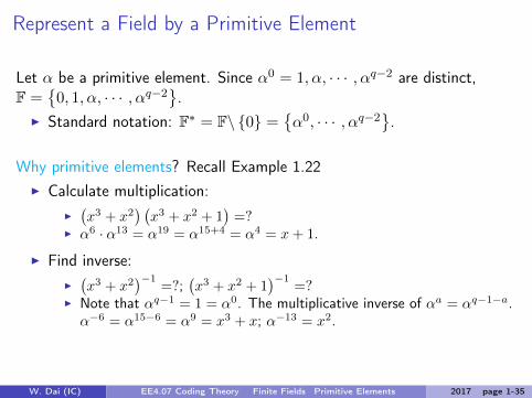
Let α be a primitive element. Since α0 = 1, α, · · · , αq−2 are distinct,F =
{0, 1, α, · · · , αq−2
}.
I Standard notation: F∗ = F\ {0} ={α0, · · · , αq−2
}.
Why primitive elements? Recall Example 1.22I Calculate multiplication:
I(x3 + x2
) (x3 + x2 + 1
)=?
I α6 · α13 = α19 = α15+4 = α4 = x+ 1.
I Find inverse:I(x3 + x2
)−1=?;
(x3 + x2 + 1
)−1=?
I Note that αq−1 = 1 = α0. The multiplicative inverse of αa = αq−1−a.α−6 = α15−6 = α9 = x3 + x; α−13 = x2.
W. Dai (IC) EE4.07 Coding Theory Finite Fields Primitive Elements 2017 page 1-35

Existence of Primitive Elements
Theorem 1.28
Every finite field Fq contains a primitive element.
To prove this theorem, we need several lemmas. After presenting andproving these lemmas, we shall prove the theorem.
W. Dai (IC) EE4.07 Coding Theory Finite Fields Primitive Elements 2017 page 1-36
Lemma 1: Fermat’s Little Theorem
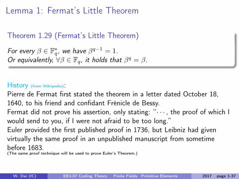
Theorem 1.29 (Fermat’s Little Theorem)
For every β ∈ F∗q , we have βq−1 = 1.Or equivalently, ∀β ∈ Fq, it holds that βq = β.
History (from Wikipedia):Pierre de Fermat first stated the theorem in a letter dated October 18,1640, to his friend and confidant Frénicle de Bessy.Fermat did not prove his assertion, only stating: “· · · , the proof of which Iwould send to you, if I were not afraid to be too long.”Euler provided the first published proof in 1736, but Leibniz had givenvirtually the same proof in an unpublished manuscript from sometimebefore 1683.(The same proof technique will be used to prove Euler’s Theorem.)
W. Dai (IC) EE4.07 Coding Theory Finite Fields Primitive Elements 2017 page 1-37

Proof of Fermat’s Little Theorem
Proof: For any β ∈ F∗q , define βF∗q = {ββ1, · · · , ββq−1}.I ββi 6= 0 ⇒ βF∗q ⊆ F∗q .
Otherwise βi = β−1ββi = β−1 · 0 = 0. A contradiction.
I ββi 6= ββj for i 6= j. ⇒∣∣βF∗q∣∣ = q − 1.
Otherwise βi = β−1 (ββi) = β−1 (ββj) = βj . A contradiction.
Hence, F∗q = βF∗q .Therefore,
∏γ∈F∗q γ =
∏γ∈βF∗q γ.
That is,β1 · β2 · · · · · βq−1= (ββ1) · (ββ2) · · · · · (ββq−1)= βq−1 · (β1 · β2 · · · · · βq−1) .
We conclude βq−1 = 1. ♦
W. Dai (IC) EE4.07 Coding Theory Finite Fields Primitive Elements 2017 page 1-38
Examples Related to Fermat’s Little Theorem
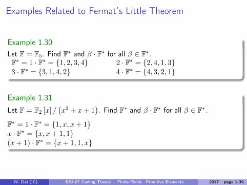
Example 1.30Let F = F5. Find F∗ and β · F∗ for all β ∈ F∗.F∗ = 1 · F∗ = {1, 2, 3, 4} 2 · F∗ = {2, 4, 1, 3}3 · F∗ = {3, 1, 4, 2} 4 · F∗ = {4, 3, 2, 1}
Example 1.31Let F = F2 [x] /
(x2 + x+ 1
). Find F∗ and β · F∗ for all β ∈ F∗.
F∗ = 1 · F∗ = {1, x, x+ 1}x · F∗ = {x, x+ 1, 1}(x+ 1) · F∗ = {x+ 1, 1, x}
W. Dai (IC) EE4.07 Coding Theory Finite Fields Primitive Elements 2017 page 1-39
Existence of Primitive Elements: Lemma 2
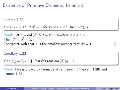
Lemma 1.32
For any β ∈ F∗, if βt = 1 for some t ∈ Z+, then ord (β) |t.
Proof: Let a = ord (β) & t = ka+ b where 0 < b < a.Then βt = βb = 1.Contradict with that a is the smallest number that βa = 1. ♦
Corollary 1.33
∀β ∈ F∗q = Fq\ {0}, it holds that ord (β) |q − 1.
Proof: This is proved by Fermat’s little theorem (Theorem 1.29) andLemma 1.32.
W. Dai (IC) EE4.07 Coding Theory Finite Fields Primitive Elements 2017 page 1-40

Existence of Primitive Elements: Lemma 3
Lemma 1.34
Suppose that ord (β1) = r1, ord (β2) = r2, and gcd (r1, r2) = 1. Letr = ord (β1β2). Then r = r1r2.
Proof:1. Since (β1β2)
r1r2 = 1, it holds r|r1r2 by Lemma 1.32.2. r1r2|r:
1 = (β1β2)rr1 = (βr11 )r βrr12 = βrr12 . Then r2|rr1. Then r2|r.
Similarly, r1|r.Hence lcm (r1, r2) |r or equivalently r1r2|r.
3. That r|r1r2 and r1r2|r implies r = r1r2. ♦
W. Dai (IC) EE4.07 Coding Theory Finite Fields Primitive Elements 2017 page 1-41
An Example Related to Lemmas 2 & 3
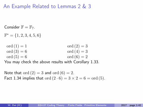
Consider F = F7.
F∗ = {1, 2, 3, 4, 5, 6}
ord (1) = 1 ord (2) = 3ord (3) = 6 ord (4) = 3ord (5) = 6 ord (6) = 2
You may check the above results with Corollary 1.33.
Note that ord (2) = 3 and ord (6) = 2.Fact 1.34 implies that ord (2 · 6) = 3× 2 = 6 = ord (5).
W. Dai (IC) EE4.07 Coding Theory Finite Fields Primitive Elements 2017 page 1-42

Existence of Primitive Elements: the Proof (1)
Proof of Theorem 1.28 (the existence):Let F∗q = {α1, · · · , αq−1} and ri = ord (αi).Define m := lcm (r1, · · · , rq−1).Based on the unique factorisation theorem (Theorem 1.9), m can bewritten as m = pk11 · · · p
k`` .
Let r1 = pk(1)1
1 · · · pk(1)`` ,
...
rq−1 = pk(q−1)1
1 · · · pk(q−1)`` .
Then ki = max(k(1)i , · · · , k(q−1)i
).
Hence, ∃αi ∈ F∗q s.t. pk11 |ord (αi):
Let β1 = αord(αi)/p
k11
i , then ord (β1) = pk11 .Similarly, find β2, · · · , β`.
W. Dai (IC) EE4.07 Coding Theory Finite Fields Primitive Elements 2017 page 1-43

Existence of Primitive Elements: the Proof (2)
Let β = β1 · · · · · β`. Clearly, ord (β) = m (Lemma 1.34).ord (βi)’s are co-prime.
Hence, m| (q − 1) (Corollary 1.33) or m ≤ q − 1.
On the other hand, by the definition of m, all q − 1 elements in F∗q areroots of xm − 1. Therefore m ≥ q − 1.
It then can be concluded that m = q − 1 and β is a primitive element. ♦
W. Dai (IC) EE4.07 Coding Theory Finite Fields Primitive Elements 2017 page 1-44

Uniqueness of Finite Fields
Definition 1.35Two fields F and G are isomorphic if there exists a one-to-one mappingϕ : F→ G that satisfies
ϕ (ab) = ϕ (a)ϕ (b) , ϕ (a+ b) = ϕ (a) + ϕ (b) .
Theorem 1.36The finite field Fq is unique up to isomorphism.
Proof is not required.
Example: F2 [x] /(x3 + x+ 1
)and F2 [x] /
(x3 + x2 + 1
)are isomorphic.
W. Dai (IC) EE4.07 Coding Theory Finite Fields Uniqueness 2017 page 1-45

Exampleϕ : F2 [x] /
(x3 + x2 + 1
)→ F2 [y] /
(y3 + y + 1
)x 7→ ϕ (x) = y + 1
ϕ : F2 [x] /(x3 + x2 + 1
)F2 [y] = y3 + y + 1
0 01 1
x y + 1
x2 y2 + 1
x2 + 1 y2
x2 + x+ 1 y2 + y + 1
x+ 1 y
x2 + x y2 + y
Verify ϕ (ab) = ϕ (a)ϕ (b):ϕ(x2 · (x+ 1)
)= ϕ
(x3 + x2
)= ϕ
(x2 + 1 + x2
)= ϕ (1) = 1.
ϕ(x2)ϕ (x+ 1) =
(y2 + 1
)· y = y3 + y = y + 1 + y = 1.
W. Dai (IC) EE4.07 Coding Theory Finite Fields Uniqueness 2017 page 1-46

Polynomial Factorisation
Problem: factorise the polynomial xqm−1 − 1 in Fq [x].
Be careful about the concept of “irreducible polynomial”:Have to specify the field we are considering.
Example 1.37Consider a polynomial M (x) = x2 + 1.1. M (x) is irreducible w.r.t. R.2. M (x) is reducible w.r.t. C: M (x) = (x+ j) (x− j).
Consider a polynomial M (x) = x2 + x+ 1.1. M (x) is irreducible w.r.t. F2.2. M (x) is reducible w.r.t. F4 = F2 [y] /y
2 + y + 1
I F4 = {0, 1, y, y + 1}.I M (x) = (x− y) (x− (y + 1)) = x2 − (y + y + 1)x+ y (y + 1).
W. Dai (IC) EE4.07 Coding Theory Finite Fields Polynomial Factorisation 2017 page 1-47

An Example of Factorisation
Factorise x3 − 1 ∈ R [x]:I Consider the easier problem: factorise x3 − 1 in C [x].I Group terms of conjugate roots
Ix3 − 1 = (x− 1)
(x− ej2π/3
) (x− ej4π/3
)= (x− 1)
(x2 + x+ 1
).
To factorise the polynomial xqm−1 − 1 in Fq [x], we use the same strategy:
I Factorise xqm−1 − 1 in Fqm [x].
I Let α be a primitive element of Fqm :
xqm−1 − 1 =
∏qm−2i=0
(x− αi
)(Irreducible polynomials in Fqm [x]).
I Group appropriate terms together:
xqm−1 − 1 =
∏sk=1M
(k) (x) (Irreducible polynomials in Fq [x]).
W. Dai (IC) EE4.07 Coding Theory Finite Fields Polynomial Factorisation 2017 page 1-48
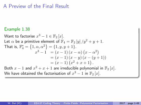
A Preview of the Final Result
Example 1.38Want to factorise x3 − 1 ∈ F2 [x].Let α be a primitive element of F4 = F2 [y] /y
2 + y + 1.That is, F∗4 =
{1, α, α2
}= {1, y, y + 1}.
x3 − 1 = (x− 1) (x− α)(x− α2
)= (x− 1) (x− y) (x− (y + 1))= (x− 1)
(x2 + x+ 1
).
Both x− 1 and x2 + x+ 1 are irreducible polynomial in F2 [x].We have obtained the factorisation of x3 − 1 in F2 [x].
W. Dai (IC) EE4.07 Coding Theory Finite Fields Polynomial Factorisation 2017 page 1-49
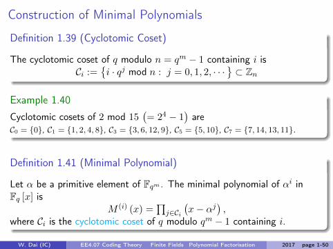
Construction of Minimal Polynomials
Definition 1.39 (Cyclotomic Coset)
The cyclotomic coset of q modulo n = qm − 1 containing i isCi :=
{i · qj mod n : j = 0, 1, 2, · · ·
}⊂ Zn
Example 1.40Cyclotomic cosets of 2 mod 15
(= 24 − 1
)are
C0 = {0}, C1 = {1, 2, 4, 8}, C3 = {3, 6, 12, 9}, C5 = {5, 10}, C7 = {7, 14, 13, 11}.
Definition 1.41 (Minimal Polynomial)
Let α be a primitive element of Fqm . The minimal polynomial of αi inFq [x] is
M (i) (x) =∏j∈Ci
(x− αj
),
where Ci is the cyclotomic coset of q modulo qm − 1 containing i.
W. Dai (IC) EE4.07 Coding Theory Finite Fields Polynomial Factorisation 2017 page 1-50
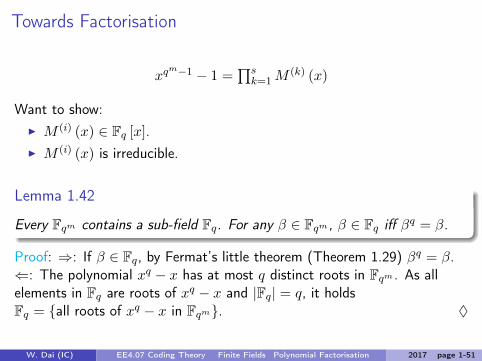
Towards Factorisation
xqm−1 − 1 =
∏sk=1M
(k) (x)
Want to show:I M (i) (x) ∈ Fq [x].I M (i) (x) is irreducible.
Lemma 1.42
Every Fqm contains a sub-field Fq. For any β ∈ Fqm , β ∈ Fq iff βq = β.
Proof: ⇒: If β ∈ Fq, by Fermat’s little theorem (Theorem 1.29) βq = β.⇐: The polynomial xq − x has at most q distinct roots in Fqm . As allelements in Fq are roots of xq − x and |Fq| = q, it holdsFq = {all roots of xq − x in Fqm}. ♦
W. Dai (IC) EE4.07 Coding Theory Finite Fields Polynomial Factorisation 2017 page 1-51
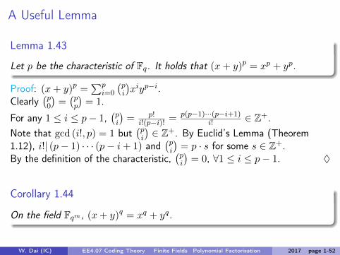
A Useful Lemma
Lemma 1.43
Let p be the characteristic of Fq. It holds that (x+ y)p = xp + yp.
Proof: (x+ y)p =∑p
i=0
(pi
)xiyp−i.
Clearly(p0
)=(pp
)= 1.
For any 1 ≤ i ≤ p− 1,(pi
)= p!
i!(p−i)! =p(p−1)···(p−i+1)
i! ∈ Z+.Note that gcd (i!, p) = 1 but
(pi
)∈ Z+. By Euclid’s Lemma (Theorem
1.12), i!| (p− 1) · · · (p− i+ 1) and(pi
)= p · s for some s ∈ Z+.
By the definition of the characteristic,(pi
)= 0, ∀1 ≤ i ≤ p− 1. ♦
Corollary 1.44
On the field Fqm , (x+ y)q = xq + yq.
W. Dai (IC) EE4.07 Coding Theory Finite Fields Polynomial Factorisation 2017 page 1-52

Properties of Cyclotomic Cosets
Lemma 1.45
Let Ci be the cyclotomic coset of q modulo qm − 1 containing i. DefineqCi := {qj mod qm − 1 : j ∈ Ci}. Then qCi = Ci.
Proof: Note that i · qm = i mod qm − 1. It is clear thatCi =
{i · qj mod qm − 1 : j = 0, 1, · · · ,m− 1
}={
i · qj mod qm − 1 : j = 1, 2, · · · ,m}= qCi. ♦
Corollary 1.46
Let α be a primitive element of Fqm . ThenM (i) (x) =
∏j∈Ci
(x− αj
)=∏j∈Ci
(x− αjq
).
Proof:∏j∈Ci
(x− αjq
)=∏`∈qCi
(x− α`
)=∏j∈Ci
(x− αj
). ♦
W. Dai (IC) EE4.07 Coding Theory Finite Fields Polynomial Factorisation 2017 page 1-53

M (i) (x) ∈ Fq [x]
Let r = |Ci|. WriteM (i) (x) =
∑` a`x
` =∏j∈Ci
(x− αj
)(a)=∑
`
(∑j1,··· ,jr−` α
j1 · · ·αjr−`)x`,
where (a) comes from the expansion of∏j∈Ci
(x− αj
). At the same
time,
M (i) (x) =∏j∈Ci
(x− αj
) (a)=∏j∈Ci
(x− αjq
)=∑
`
(∑j1,··· ,jr−` α
j1q · · ·αjr−`q)x`
(b)=∑
`
(∑j1,··· ,jr−` α
j1 · · ·αjr−`)qx`
=∑
` aq`x`,
where (a) comes from Corollary 1.46, (b) comes from Corollary 1.44.Hence, a` = aq` , which implies a` ∈ Fq and M (i) (x) ∈ Fq [x]. ♦
W. Dai (IC) EE4.07 Coding Theory Finite Fields Polynomial Factorisation 2017 page 1-54

M (i) (x) is Irreducible
Step 1: For all f (x) ∈ Fq [x] s.t. f(αi)= 0, it holds that M (i) (x) |f (x).
Write f (x) = f0 + f1x+ · · ·+ fnxn.
For any j ∈ Ci, ∃` s.t. j = iq` mod qm − 1.
f(αj)
= f(αiq
`)= f0 + f1α
iq` + · · ·+ fnαiq`·n
= f q`
0 + f q`
1 αiq` + · · ·+ f q
`
n αiq`·n
=(f0 + f1α
i + · · ·+ fnαin)q`
= f(αi)q`
= 0.
That is, αj is also a root of f . Hence, M (i) (x) |f (x).
Step 2: M (i) (x) is irreducible in Fq [x].Suppose not. Then M (i) (x) = g (x)h (x) for nontrivial g (x) and h (x).αi is a root of M (i) (x) ⇒ αi is a root of one of g (x) and h (x).W.l.o.g., αi is a root of g (x). Then M (i) (x) |g (x) which is impossible.Hence M (i) (x) is irreducible. ♦
W. Dai (IC) EE4.07 Coding Theory Finite Fields Polynomial Factorisation 2017 page 1-55

Representatives of Cyclotomic Cosets
Definition 1.47Consider the cyclotomic cosets of q mod n.A subset {i1, · · · , ij} ⊂ Zn is a complete set of representatives ofcyclotomic cosets if
Ci1⋃· · ·⋃Cij = Zn.
Example 1.48Cyclotomic cosets of 2 mod 15 areC0 = {0}, C1 = {1, 2, 4, 8}, C3 = {3, 6, 12, 9}, C5 = {5, 10}, C7 = {7, 14, 13, 11}.The complete set of representatives is {0, 1, 3, 5, 7}.
W. Dai (IC) EE4.07 Coding Theory Finite Fields Polynomial Factorisation 2017 page 1-56

Factorisation
Theorem 1.49Let α be a primitive element of Fqm . Let {i1, · · · , is} be a complete set ofrepresentatives of cyclotomic cosets of q modulo qm − 1. Then
xqm−1 − 1 =
∏qm−2i=0
(x− αi
)=∏sk=1M
(ik) (x) .
Proof:The first equality: The degrees are the same. The coefficients beforexq
m−1 are the same. The roots are also the same.The second equality: holds from the definitions of M (ik) (x) and thecomplete set of representatives. ♦
W. Dai (IC) EE4.07 Coding Theory Finite Fields Polynomial Factorisation 2017 page 1-57

Section 2Cryptography
I IntroductionI Password management: store, exchange, and secret shareI The public key cryptography
I The RSA cryptosystemI The ElGamal cryptosystem
I Digital signatureThe contents are heavily based on Biggs’ book, Chapters 13 & 14.
W. Dai (IC) EE4.07 Coding Theory Cryptography 2017 page 2-1

Cryptography
Definition 2.1 (Cryptography)A framework of cryptography includes a set of plaintext messagesM, a setof ciphertext messages C, and a set of keys K. For each k ∈ K, there is anencryption function Ek : M→ C and the corresponding decryptionfunction D` : C →M such that
D` (Ek (m)) = m, for all m ∈M.
W. Dai (IC) EE4.07 Coding Theory Cryptography Introduction 2017 page 2-2

Cryptography: An Example
One of the oldest cryptographic systems is said to have been used by JuliusCaesar over two thousand years ago.Let A be the English alphabet set. Let K = {1, 2, · · · , 25}. For a given keyk ∈ K, replace each letter by the one that is k places later.For example, if k = 5, then the message
SEE␣YOU␣TOMORROW becomes XJJ␣DTZ␣YTRTWWTB
For the Caesar system, a simple attack is exhaustive search as there areonly 25 keys.A natural extension is to use any permutation of 26 letters, yielding26! ≈ 4× 1027 keys. Exhaustive search is impossible.
However, in this case another method, called frequency analysis, is a muchmore effective attack.It uses the observation that the frequencies of the English letters are fairlyconstant over a wide range of texts.
W. Dai (IC) EE4.07 Coding Theory Cryptography Introduction 2017 page 2-3

Another Example: Hill’s Cryptography System
Consider a 29-symbol alphabet including 26 English letters, the space ␣,comma, and full stop. It is mapped to F29.Given a stream of symbols, split it into blocks of size n so that each blockcan be written as m ∈ Fn29. A key K ∈ Fn×n29 is an invertible matrix. Theencryption function is given by
c =Km,
and the decryption function is
m =K−1c.
W. Dai (IC) EE4.07 Coding Theory Cryptography Introduction 2017 page 2-4

Diagram of Cryptography Systems
Adapted from http://www.akadia.com/services/email_security.html
I Popular cryptography systems are built on large prime numbers.I Symmetric cryptography: encryption key k = decryption key `.I Asymmetric cryptography: k 6= `.
W. Dai (IC) EE4.07 Coding Theory Cryptography Introduction 2017 page 2-5

Existence of Large Prime Numbers
Theorem: There exist infinitely many prime numbers.
Proof:1. Suppose that there exist only finitely many prime numbers.2. List all these prime numbers, p1, p2, · · · , pN .3. Let x = p1 · p2 · · · pN + 1.4. Claim: x is a prime number.
Proved by the Unique Factorisation Theorem 1.9 as gcd (pi, x) = 1.5. This contradicts the assumption that the list of p1, p2, · · · , pN
contains all the prime numbers. ♦
W. Dai (IC) EE4.07 Coding Theory Cryptography Prime Numbers 2017 page 2-6

Large Prime Numbers
A list of large prime numbers (http://primes.utm.edu)
Prime When Prime When Prime When257885161 − 1 2013 243112609 − 1 2008 242643801 − 1 2009237156667 − 1 2008 232582657 − 1 2006 230402457 − 1 2005
Large prime numbers matter:To check whether a 64bit number is a prime or not by brute force,
how long will it take?
Assume a computer can evaluate 1G (109) “basic operations” per second.264/(109 · 3600 · 24 · 365) ≈ 585 years!
Nowadays, a prime number between 512b and 1024b is often used.Any brute force method is impractical!
W. Dai (IC) EE4.07 Coding Theory Cryptography Prime Numbers 2017 page 2-7

How to Store Passwords on a Server?
I A set of users wish to log in securely to a server.I Each user choose a password.I The passwords are stored in a file
I Should not be saved in the ‘raw’ format.I Easy to check whether a password is valid.I Very difficult to extract the passwords from the file.
Solution: use the discrete logarithmic function.
W. Dai (IC) EE4.07 Coding Theory Cryptography Store Passwords 2017 page 2-8

The Discrete Logarithm
Normal exponential function:x 7→ y = bx,
Normal logarithmic function:y 7→ x = logb y.
It can be solved by Taylor expansion efficiently.
Definition 2.2 (Discrete logarithm problem (DLP))Let p be a prime number and b ∈ F∗p be a primitive element.For any given y ∈ F∗p, find the x ∈ F∗p such that
y = bx (mod p).
I It is well-defined if and only if b is primitive.
W. Dai (IC) EE4.07 Coding Theory Cryptography Store Passwords 2017 page 2-9

Computation Complexity
Discrete exponential function: computational complexity O (log (p))Example: 3211 =? (mod 811)Note that 211 = 128 + 64 + 16 + 2 + 1.One has 3211 = 3128 · 364 · 316 · 32 · 31 (mod 811).It can be achieved by computing32 = 3 · 3 (mod 811), 34 = 32 · 32 (mod 811),· · · , 32k = 32
k−1 · 32k−1(mod 811).
Discrete logarithmic function: computational complexity O (p).I It is usually solved by brute force search.
I No sufficiently efficient algorithm in general.
W. Dai (IC) EE4.07 Coding Theory Cryptography Store Passwords 2017 page 2-10

Examples
Let p = 811 and b = 3.The output of discrete logarithmic function looks random:log3 2 = 717; log3 3 = 1; log3 4 = 624; log3 5 = 494; · · · .
0 100 200 300 400 500 600 700 8000
1
2
3
4
5
6
7
x
y=lo
g(x)
Normal Logarithmic Function: b=3
0 100 200 300 400 500 600 700 8000
100
200
300
400
500
600
700
800
x
y=dl
og(x
) (m
od p
)
Discrete Logarithmic Function: p=811, b=3
W. Dai (IC) EE4.07 Coding Theory Cryptography Store Passwords 2017 page 2-11

Store Passwords on a Server: A Solution
I The administrator chooses a prime p and a primitive element b.I The values of p and b are also kept on the server.
I The user i chooses a password. This is converted into a numberxi ∈ F∗p.
I Let yi = bxi (mod p) and the pair (i, yi) is stored.
W. Dai (IC) EE4.07 Coding Theory Cryptography Store Passwords 2017 page 2-12

Cryptography for Information Exchange
In the previous scheme:Decoding is difficult for everyone.
In the information exchange scenario, for example, Alice sends somemessage to Bob.Alice’s information to Bob should be encrypted.Bob would like to be able to decrypt the message easily.
The traditional choice: Symmetric cryptographyThe encryption and decryption keys are the same, i.e., k = `.The keys are known to both Alice and Bob for encryption and decryptionrespectively.Disadvantages: A secure channel is needed for key exchange.Disasters may happen if the key is leaked.
W. Dai (IC) EE4.07 Coding Theory Cryptography Encryption Key Exchange 2017 page 2-13

Symmetric Key Cryptography
From http://chrispacia.wordpress.com/2013/09/07/bitcoin-cryptography-digital-signatures-explained/
The key is to keep the key safe.
W. Dai (IC) EE4.07 Coding Theory Cryptography Encryption Key Exchange 2017 page 2-14

Key Exchange
Problem: Alice and Bob want to share a secret key but their informationexchange could be observed by their adversary Eve. How is it possible forAlice and Bob to share a key without making it known to Eve?
Solution: Diffie-Hellman key exchange.Wikipedia: The scheme was first published by Whitfield Diffie and Martin Hellman in 1976, although it had beenseparately invented a few years earlier within GCHQ, the British signals intelligence agency, by James H. Ellis,Clifford Cocks and Malcolm J. Williamson but was kept classified.
W. Dai (IC) EE4.07 Coding Theory Cryptography Encryption Key Exchange 2017 page 2-15

Diffie-Hellman Key Exchange
1. Alice and Bob agree on a large prime p and an integer g mod p. Thevalues of p and g are publicly known.
2. Alice picks a secret integer a that she does not reveal to anyone, andBob picks an integer b that he keeps secret. They compute
A = ga mod p, and B = gb mod p,
respectively. They next exchange these computed values.Note that Eve sees the values of A and B.
3. Alice and Bob uses their secret integers to compute
A′ = Ba mod p, and B′ = Ab mod p,
respectively. Note that A′ = B′ = gab is the shared secret key forinformation exchange.
W. Dai (IC) EE4.07 Coding Theory Cryptography Encryption Key Exchange 2017 page 2-16

Secret Share: Motivation
Secrecy-reliability tradeoff in storing an encryption keyI Maximum secrecy: keep a single copy of the key in one location
I What if it gets lost.
I Reliability: store multiple copies at different locationsI What if a copy falls into the wrong hand.
Secret Sharing: (k, n) threshold scheme.Store the secret S into n pieces of encrypted words S1, · · · , Sn such thatI Knowledge of any K or more Si pieces makes S easily computable.I Knowledge of any k − 1 or fewer Si pieces leaves S undetermined.
W. Dai (IC) EE4.07 Coding Theory Cryptography Secret Share 2017 page 2-17

Shamir’s Secret Sharing
Idea of Adi Shamir’s threshold scheme: k points to define a polynomial ofdegree k − 1. 2 points are sufficient to define a line, 3 points are sufficient to define aparabola, 4 points to define a cubic curve and so forth.
A (k, n) threshold scheme to share our secret S:1. Let p be a prime number. Let n < p and S < p.2. Randomly choose k − 1 positive integers a1, · · · , ak−1. Set a0 = S.3. Set f (x) = a0 + a1x+ a2x
2 + · · ·+ ak−1xk−1.
4. Evaluate f (x) at n points to obtain (ti, f (ti)), ti ∈ F∗p andi = 1, · · · , n.
Claim: given any k such pairs (ti, f (ti)), we can find the coefficients of thepolynomial and therefore a0.
W. Dai (IC) EE4.07 Coding Theory Cryptography Secret Share 2017 page 2-18
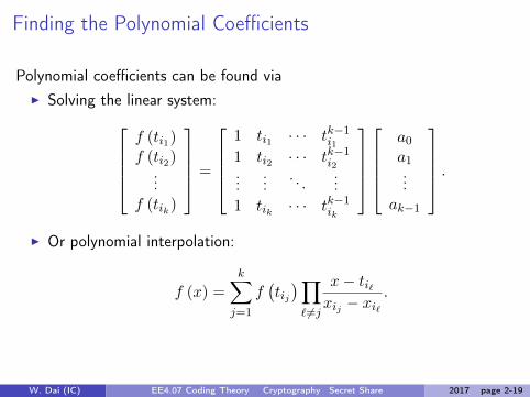
Finding the Polynomial Coefficients
Polynomial coefficients can be found viaI Solving the linear system:
f (ti1)f (ti2)
...f (tik)
=
1 ti1 · · · tk−1i1
1 ti2 · · · tk−1i2...
.... . .
...1 tik · · · tk−1ik
a0a1...
ak−1
.I Or polynomial interpolation:
f (x) =
k∑j=1
f(tij)∏` 6=j
x− ti`xij − xi`
.
W. Dai (IC) EE4.07 Coding Theory Cryptography Secret Share 2017 page 2-19

Cryptography for Information Exchange (2)A modern solution: Public key algorithms (Asymmetric Cryptography)
Encryption key k 6= ` decryption key.The encryption key is public while the decryption key is kept secret.
From http://www.akadia.com/services/email_security.html
W. Dai (IC) EE4.07 Coding Theory Cryptography Public Key Cryptography 2017 page 2-20

ComparisonComparisons of asymmetric cryptography over the symmetric one.Advantages:I No secret channel is necessary for the key exchange.I Less key-management problems. Only 2n keys are needed for n
entities to communicate securely with one another (each entitymaintains a private key and a public key). In a system based onsymmetric ciphers, you would need
(n2
)= n (n− 1) /2 secret keys
(each pair of entities agrees on a key).I More robust to “brute-force” attack in which all possible keys are
attempted.I Can provide digital signatures.
Disadvantages:I Much slower. The computational complexity of asymmetric
cryptography is much larger.In practice, these two schemes are rarely used exclusively. For example,your browser encrypts a symmetric key using the server’s public key.
W. Dai (IC) EE4.07 Coding Theory Cryptography Public Key Cryptography 2017 page 2-21

The ElGamal Cryptography
Key generation:I Choose a prime p and a primitive element b ∈ F∗p.I Private key: choose an integer a′ ∈ N.I Public key: a = ba
′ ∈ F∗p.
Encryption: Alice transmits her public key a to Bob and keeps the privatekey a′ secret. Bob randomly choose t ∈ N and encrypt the message m to(
bt, mat)
Decryption: Alice can recover m viam = mat
(bt)−a′
= mata−t mod p.
Advantage:The random number t generates a random encryption function.
W. Dai (IC) EE4.07 Coding Theory Cryptography Public Key Cryptography 2017 page 2-22

RSA Cryptography
RSA public key cryptography:Published in 1977 by Ron Rivest, Adi Shamir, and Leonard Adleman at MIT.
Key generation:I Choose primes p1 6= p2. Let n = p1p2 and t = (p1 − 1) (p2 − 1).I Public key: (n, e) where 1 < e < t and gcd (e, t) = 1.I Private key: d where 1 < d < t and d · e mod t = 1.
I Find d by the Euclidean algorithm.
Encryption: Bob sends his public key (n, e) to Alice and keeps the privatekey d secret. Alice encrypts the message m to c via
c = me mod n.
Decryption: Bob can recover m from c viam = cd mod n
W. Dai (IC) EE4.07 Coding Theory Cryptography Public Key Cryptography 2017 page 2-23

An Example
I Bob chooses p1 = 47 and p2 = 59.I n = 47× 59 = 2773. t = 46× 58 = 2668.I e = 157 is a valid public key as gcd (e, 2668) = 1.I Use Euclidean algorithm, d = 17.I To send a message m = 5, Alice computes the ciphertext
c = me = 5157 = 1044 (mod 2773).I Bob deciphers the ciphertext via
m̂ = cd = 104417 = 5 (mod 2773),which is the correct message.
W. Dai (IC) EE4.07 Coding Theory Cryptography Public Key Cryptography 2017 page 2-24

Theory Behind RSA
Recall Fermat’s Little Theorem (Thm 1.29): ∀a ∈ F∗p, ap−1 = 1 mod p
Theorem 2.3 (Euler’s Theorem)
Let p1 6= p2 be two prime numbers. Define n := p1p2 andt := (p1 − 1) (p2 − 1). Then ∀a ∈ Z+,
akt+1 = a mod n, ∀k ≥ 0
The correctness of RSA:(me)d = med = mqt+1 = mqt ·m = m mod n.
W. Dai (IC) EE4.07 Coding Theory Cryptography Public Key Cryptography 2017 page 2-25

Proof of Euler’s Theorem: A Lemma
With a slight abuse of notation, define x = y mod p if |x− y| = 0 mod p.
Lemma 2.4
For any two positive integers x and y, if x = y mod p1 and x = y mod p2,then x = y mod p1p2.
Proof: Since x = y mod p1 and x = y mod p2, it is clear thatx− y = k1p1 = k2p2 for some integers k1 and k2.By Euclid’s Lemma (Lemma 1.12), p2| (p1k1) and gcd (p2, p1) = 1 implythat p2|k1, or equivalently k1 = k3p2 for some integer k3.Hence, x− y = (k3p2) p1 and x ≡ y mod p1p2. ♦
W. Dai (IC) EE4.07 Coding Theory Cryptography Public Key Cryptography 2017 page 2-26

Proof of Euler’s Theorem
Fix an a ∈ {1, 2, · · · , p1p2 − 1}.I We first show that ade = a mod p1.
If p1|a, then it is clear that ade = a+(ade − 1
)a = a mod p1.
If p1 - a, then by Fermat’s Little Theorem (Thm 1.29)ap1−1 ≡ 1 mod p1 and therefore ade ≡ ak(p1−1)(p2−1)+1 ≡ a mod p1.
I Similarly ade = a mod p2.I Hence ade = a mod p1p2.
Euler’s Theorem is therefore proved. ♦
W. Dai (IC) EE4.07 Coding Theory Cryptography Public Key Cryptography 2017 page 2-27
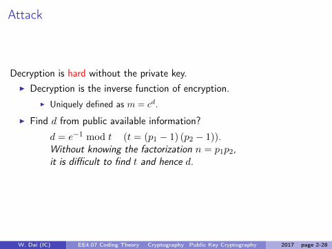
Attack
Decryption is hard without the private key.I Decryption is the inverse function of encryption.
I Uniquely defined as m = cd.
I Find d from public available information?
d = e−1 mod t (t = (p1 − 1) (p2 − 1)).Without knowing the factorization n = p1p2,it is difficult to find t and hence d.
W. Dai (IC) EE4.07 Coding Theory Cryptography Public Key Cryptography 2017 page 2-28

Digital Signature: The General Principle
Problem:I Alice wishes to send a message m to Bob.I Bob would like to verify that the message comes from Alice.
In physical world, Alice sign the letter.In digital world, any fixed signature can be easily copied.
General principle:I Alice sends (m, y = s (m)),
I y = s (m) is the message dependent signature.I The signature function s should kept secret.
I Bob checks whether m = s−1 (y).I He doesn’t know the signature function s.
W. Dai (IC) EE4.07 Coding Theory Cryptography Digital Signature 2017 page 2-29
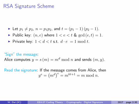
RSA Signature Scheme
I Let p1 6= p2, n = p1p2, and t = (p1 − 1) (p2 − 1).I Public key: (n, e) where 1 < e < t & gcd (e, t) = 1.I Private key: 1 < d < t s.t. d · e = 1 mod t.
“Sign” the message:Alice computes y = s (m) = md mod n and sends (m, y).
Read the signature: If the message comes from Alice, thenye =
(md)e
= mkt+1 = m mod n.
W. Dai (IC) EE4.07 Coding Theory Cryptography Digital Signature 2017 page 2-30

Extend ElGamal Cryptography to ElGamal Signature?
RSA based schemes:I In cryptography, we have D` (Ek (m)).I In digital signature, we have Ek (D` (m)).I This works as (me)d =
(md)e.
This principle cannot be directly applied to ElGamal scheme.
W. Dai (IC) EE4.07 Coding Theory Cryptography Digital Signature 2017 page 2-31
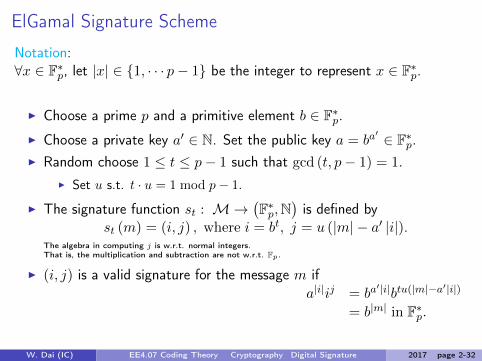
ElGamal Signature Scheme
Notation:∀x ∈ F∗p, let |x| ∈ {1, · · · p− 1} be the integer to represent x ∈ F∗p.
I Choose a prime p and a primitive element b ∈ F∗p.I Choose a private key a′ ∈ N. Set the public key a = ba
′ ∈ F∗p.I Random choose 1 ≤ t ≤ p− 1 such that gcd (t, p− 1) = 1.
I Set u s.t. t · u = 1 mod p− 1.
I The signature function st : M→(F∗p,N
)is defined by
st (m) = (i, j) , where i = bt, j = u (|m| − a′ |i|).The algebra in computing j is w.r.t. normal integers.That is, the multiplication and subtraction are not w.r.t. Fp.
I (i, j) is a valid signature for the message m ifa|i|ij = ba
′|i|btu(|m|−a′|i|)
= b|m| in F∗p.
W. Dai (IC) EE4.07 Coding Theory Cryptography Digital Signature 2017 page 2-32

Summary
I Factorize a product of two large prime numbersI RSA public key cryptographyI RSA signature scheme
I Discrete logarithm problemI Store passwordsI Diffie-Hellman key exchangeI ElGamal public key cryptographyI ElGamal signature scheme
I PolynomialI Secret share
W. Dai (IC) EE4.07 Coding Theory Cryptography Summary 2017 page 2-33