ee414 - performance evaluation of queuing systemsee414/notes/ee414-09-slides-4.pdf · queuing...

Performance Evaluation ofQueuing Systems

Introduction to Queuing SystemsSystem Performance Measures & Little’s LawEquilibrium Solution of Birth-Death Processes

Analysis of Single-Station Queuing Systems

Dr Conor McArdle EE414 - Performance Evaluation of queuing Systems 1/1

Single Station Queuing Systems

Single station queuing models are useful for performance evaluation of many devices,sub-systems and communications nodes that make up communications networks.

We introduce the different types of queuing systems that are possible and then presentBirth-Death models that allow us to compute performance measures, such as meanqueue length and delay, for such systems.

Queuing System Models

In a single station queuing model, the queuing system consists of a buffer for queuingcustomers and one or more identical servers. The queue may be of zero, finite orinfinite size.

1

ArrivingCustomers

DepartingCustomers

mQueue

Servers


Queuing Systems

A server may only serve one “customer” (packet, call, request, etc.) at a time and so,at any given time, it is either “busy” or “idle”.

A customer represents some unit of work that keeps a server busy for some amount oftime - (e.g. transmission of a packet of some length, carrying of a call for someamount of time, processing of a request, etc.).

If all servers in the system are busy when a new customer arrives then the customerjoins the queue, if there is remaining space in the queue.

When a customer finishes service, it departs the system and a new customer is selectedfrom the queue (if there are any waiting) to begin its service.

There are two sources of randomness in such a system:

1 customers arrive at random times, that is, the inter-arrival-time of customers isdescribed by a random variable.

2 the amount of time required to service a customer is random, that is, the servicetime is described by a random variable.

It is often assumed that arrivals are independent events and that the service times ofdifferent customers are also independent.


Queuing Systems - Kendall’s Notation

Kendall’s Notation for Queues

We use the following notation to describe different types of queuing systems:

A/B/m/K/p− queuing discipline

A is the distribution of inter-arrival times and B is the distribution of service times.

The distributions A and B may be indicated as:

M - Exponentially distributed inter-arrival times or service times (where the Mindicates Memoryless)

D - Deterministic distribution (that is, constant)

G - General distribution (of unknown distribution)

GI - General independent (unknown distribution but with independent arrivalsand service times).

For the distributions A and B above, the mean arrival rate is normally denoted as λand the mean service time as 1/µ, that is, µ is the mean service rate.


Queuing Systems - Kendall’s Notation

m indicates the number of servers in the system.

K indicates the capacity of the overall system (the number of queuing places plus thenumber of servers). If K is not specified in the Kendall notation, then the bufferingcapacity (queue length) is taken as infinite.

p indicates the number in the population of customers that may arrive to the system,that is, the number of users of the system. If p is not specified in the notation, thenthe population is taken as infinite.

The queuing discipline determines which customer is selected from the queue forprocessing when a server becomes available. Examples of different queuing disciplinesare:

FCFS - First-Come-First-Served - If no queuing discipline is stated in theKendall description, this one is assumed. All the systems we consider have aFCFS queuing discipline.

LCFS - Last-Come-First-Served

PS - Processor-Sharing: All customers are served simultaneously where processingof all customers is equally spread across all servers.



Introduction to Queuing SystemsSystem Performance Measures & Little’s Law

Equilibrium Solution of Birth-Death ProcessesAnalysis of Single-Station Queuing Systems


Queuing Systems - Performance Measures

We now introduce some notation for the performance measures of interest in queuingsystems.

Number of Customers in the System: In steady-state, the expected value ofthe state distribution vector {πk} gives the mean number of customers in thesystem. We will find a solution for the stationary distribution {πk} forcontinuous-time Birth-Death processes (queuing systems) later in this section.Given {πk}, many of the other performance measures of interest may be derived.

Utilisation (ρ): For a queuing system with a single server, utilisation ρ is thefraction of time the server is busy. When there is no limit on the capacity of thesystem, then

ρ =mean service time

mean inter-arrival time=

arrival rate

service rate=λ

µ.

The utilization ρ when there are multiple servers, is the mean fraction of busyservers. Since mµ is the overall service rate, in this case we have

ρ =λ

mµ.

For a stable (ergodic) system, the condition for stability is ρ < 1.


Queuing Systems - Performance Measures

Throughput (λ): The throughput for a queuing system with infinite capacity isthe mean number of customers processed in a unit of time, i.e. the departurerate. Since the departure rate is equal to the arrival rate (and assuming ρ < 1),the throughput is

λ = m · ρ · µ.For a queuing system with finite capacity, there can be loss in the systems, and sothe throughput can be less than the arrival rate. In this case, throughput is oftendenoted differently (e.g. as S) to distinguish it from the arrival rate λ.

Response Time (T ): (or sojourn time) is the total time a customer spends inthe system.

Waiting Time (W ): is the time a job spends in the queue waiting to be serviced.Therefor, response time is the sum of the waiting time and the service time for acustomer. T and W are, in general, random variables, so the expected values (T̄and W̄ ) are often used and we may write:

T̄ = W̄ +1µ.

Number of Customers in the System (N): Again N is a random variable andits expected value N̄ is often of interest:

N̄ =∑∞

k=1 k · πkDr Conor McArdle EE414 - Performance Evaluation of queuing Systems 8/1

Little’s Law

The mean number of customers in the system N̄ and the mean response time T̄ canbe related using one of the most important theorems of queuing theory, Little’s Law:

N̄ = λT̄

We outline a proof of the Little’s theorem as follows:

Let α(t) , the number of arrivals in the time interval (0, t)Let δ(t) , the number of departures in the time interval (0, t)

N(t)

á(t)

ä(t)

1

2

3

4

5

6

7

8

9

0Time t

Number of

Customers


Little’s Law

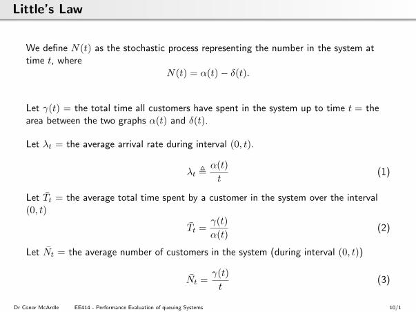
We define N(t) as the stochastic process representing the number in the system attime t, where

N(t) = α(t)− δ(t).

Let γ(t) = the total time all customers have spent in the system up to time t = thearea between the two graphs α(t) and δ(t).

Let λt = the average arrival rate during interval (0, t).

λt ,α(t)t

(1)

Let T̄t = the average total time spent by a customer in the system over the interval(0, t)

T̄t =γ(t)α(t)

(2)

Let N̄t = the average number of customers in the system (during interval (0, t))

N̄t =γ(t)t

(3)


Little’s Law

Equations (1),(2) and (3) can be combined:

γ(t)t

=α(t)t.γ(t)α(t)

N̄t = λtT̄t

Let λ = Limt→∞ λt and T̄ = Limt→∞ T̄t

N̄ will then also exist giving N̄ = λT̄ .

The above result does not depend on the inter-arrival or service time distributions or onthe number of servers in the system. Also, the law applies to any arbitrary boundaryaround part of the system, for example if only the queue is being considered then

N̄q = λW̄ ,

where N̄q is the average number of customers in the queue and W̄ is the average timespent waiting in the queue. If only the server is being considered then:

N̄s =λ

µ.



Introduction to Queuing SystemsSystem Performance Measures & Little’s Law

Equilibrium Solution of Birth-Death ProcessesAnalysis of Single-Station Queuing Systems


Birth-Death Systems in Equilibrium

We may model many different types of queuing systems by applying ourcontinuous-time Birth-Death (Markov chain) analysis methods.

Calculation of the performance measures of interest depends on resolution of thestationary distribution of the states of the process, {πk}.

We have previously resolved the transient solution of the Birth-Death system for thesimple case of the Poisson process. We now turn to the equilibrium solution and, giventhat the equations are more straight-forwards, we may find a general solution to {πk}in terms of the birth and death coefficients.

Recall that the stationary distribution of an ergodic, homogeneous, continuous-timeMarkov chain is given by the solution to the system of linear equations:

0 = πQ (4)

coupled with the normalisation condition:

π1T =∑∀i∈S

πi = 1



From our definition of a Birth-Death process, recall that the matrix of transition ratesQ takes the form:

Q =

−λ0 λ0 0 0 . . .µ1 −(λ1 + µ1) λ1 0 . . .0 µ2 −(λ2 + µ2) λ2 . . .0 0 µ3 −(λ3 + µ3) . . ....

......

.... . .

And so, equation (4) gives the set of linear equations:

0 = −(λk + µk)πk + λk−1πk−1 + µk+1πk+1 k ≥ 1 (5)

0 = −λ0π0 + µ1π1 k = 0 (6)

So as to eliminate the equation for k = 0, we put

λ−1 = λ−2 = λ−3 = . . . = 0µ0 = µ−1 = µ−2 = . . . = 0

Since a negative number of customers in the system is not possible, we have

π−1 = π−2 = π−3 = . . . = 0.



Thus, equations (5) and (6) can be combined to give the equilibrium equation:

0 = −(λk + µk)πk + λk−1πk−1 + µk+1πk+1 k = . . .− 2,−1, 0, 1, 2, . . . (7)

We find a solution for πk as follows:

Solving for π1

π1 =λ0

µ1π0

Solving for π2

0 = −(λ1 + µ1)π1 + λ0π0 + µ2π2

0 = −(λ1 + µ1)λ0

µ1π0 + λ0π0 + µ2π2

0 = −λ1λ0

µ1π0 − λ0π0 + λ0π0 + µ2π2

⇒ π2 =λ0λ1

µ1µ2π0



Continuing in this way:

πk =λ0λ1 . . . λk−1

µ1µ2 . . . µkπ0

Thus the equilibrium probabilities may be expressed as:

πk = π0

k−1∏i=0

λiµi+1

k = 0, 1, 2, . . . (8)

And using the conservation (normalisation) equation, and noting that an emptyproduct is equal to 1:

π0 =1

1 +∞∑k=1

[k−1∏i=0

λiµi+1

] (9)

Equations (8) and (9) give the general equilibrium (stationary) solution of theBirth-Death process.

We may model different types of queuing systems (as previously described by theKendall notation) simply by setting particular sets of values for the coefficients λi, µi.



Introduction to Queuing SystemsSystem Performance Measures & Little’s LawEquilibrium Solution of Birth-Death Processes

Analysis of Single-Station Queuing Systems


M/M/1 Queuing System

In this case of an M/M/1 queuing system, the Birth-Death coefficients are:

λk = λ k = 0, 1, 2, . . .µk = µ k = 1, 2, 3, . . .

0

ì

1

ë

2 k-1 k k+1

ë

ì ì

ë ëë ë

ì ì ì

ë

ì

Solving with these coefficients using the general solution equation (8):

pk = p0

k−1∏i=0

λ

µ

pk = p0

(λ

µ

)kk ≥ 0

Note the change in notation to agree with Kleinrock: pk ≡ πk



Calculating p0 using the normalisation equation (9):

p0 =

[1 +

∞∑k=1

(λ

µ

)k]−1

p0 =[1 +

λ/µ

1− λ/µ

]−1

p0 = 1− λ/µ

Combining:

pk = (1− ρ)ρk k = 0, 1, 2, . . . where ρ = λ/µ

Note that for stability (ergodicity) in this system: ρ < 1.

To calculate N̄ the average number of customers in the system:

N̄ =∞∑k=0

k pk

N̄ =ρ

1− ρ



pk

5

k1 2 4 6 7 83

Figure: The steady state probability of k customers in the system (pk) for a given value ofρ < 1

We can now calculate the average time spent in the system using Little’s Law:

T̄ =N̄

λ=

ρ

1− ρ1λ

T̄ =1/µ

1− ρ



From the definition of the system, the arrivals to the M/M/1 system form a Poissonprocess, that is, the inter-arrival times are exponentially distributed.

We note (without proof) that the output process of the M/M/1 system is also aPoisson process, that is, the ‘inter-departure’ times are also exponentially distributed,with the same parameter λ as the inter-arrival times.

We further note that the combination of Poisson traffic streams is also a Poissontraffic stream (see Tutorial 2).

These facts make it easy to analyse networks of connected M/M/1 systems, where thearrival process to one node is formed by the departure streams from one or more othernodes.

For other types of queuing systems, it is generally not the case that the departureprocess is the same as the arrival process and network analysis problems then involveresolving the joint distributions of the states of multiple queuing stations (generally anintractible problem to solve exactly for a large number of nodes).


Queuing System with Discouraged Arrivals

Consider a queuing system where arrivals are discouraged when more customers arepresent in the system. This may be represented using state-dependent arrival (birth)rates in the Birth-Death system:

λk =α

k + 1k = 0, 1, 2, . . .

µk = µ k = 1, 2, 3, . . .

0

ì

1

á/2

2 k-1 k k+1

á

ì ì

á/3 á/ká/( -1)k á/( +1)k

ì ì ì

á/( +2)k

ì

Solving for pk and p0:

pk = p0

k−1∏i=0

α/(i+ 1)µ

= p0

(α

µ

)k 1k!

p0 =

[1 +

∞∑k=1

(α

µ

)k 1k!

]−1

= e−α

µ

Combining gives: pk =(α/µ)k

k!e−α

µ k = 0, 1, 2, . . .


M/M/m Queuing System

Consider a system with unlimited buffering capacity and m servers. The Birth-Deathcoefficients are:

λk = λ k = 0, 1, 2, . . .

µk ={kµ 0 ≤ k ≤ mmµ m ≤ k

0

ë

1 m-2 m-1 m+1

ì 2ì

ë ëë ë

(m-2)ì (m-1)ì mì

ë

mì

m

ë

mì

Note that, for an ergodic systemλ

mµ< 1

For the range k ≤ m : pk = p0

k−1∏i=0

λ

(i+ 1)µ= p0

(λ

µ

)k 1k!

For the range k ≥ m : pk = p0

m−1∏i=0

λ

(i+ 1)µ

k−1∏j=m

λ

mµ= p0

(λ

µ

)k 1m!mk−m



Combining we have:

pk =

p0

(mρ)k

k!k ≤ m

p0ρkmm

m!k ≥ m

Where ρ =λ

mµ< 1

p0 =

[m−1∑k=0

(mρ)k

k!+∞∑k=m

ρkmm

m!

]−1

=

[m−1∑k=0

(mρ)k

k!+(

(mρ)m

m!

)(1

1− ρ

)]−1

The probability that an arrival joins the queue (is not served immediately) is:

P [queuing] =∞∑k=m

pk =∞∑k=m

p0ρkmm

m!

P [queuing] =

((mρ)m

m!

)(1

1− ρ

)[m−1∑k=0

(mρ)k

k!+(

(mρ)m

m!

)(1

1− ρ

)]Dr Conor McArdle EE414 - Performance Evaluation of queuing Systems 24/1


The above equation is known as Erlang’s C Formula.

As it is can be cumbersome to calculate, charts (or software) are used to find valuesfor the probability of delay (queuing).

We may also use the formula (by way of charts or software) to find the number ofservers required given the maximum allowable probability of delay for a given thearrival intensity.

The Erlang-C formula is charted on the next slide. The x-axis is the traffic intensity,a measure of the rate of work offered to the system.

For a single server system:

Traffic Intensity = ρ = λ · 1µ

For an m server system:

Traffic Intensity = m · ρ = λ · 1µ

The unit of traffic intensity is the Erlang, a dimensionless quantity.



1 2 3 4 5 6 7 8 9 100.001

0.002

0.5 1.5 2.5 3.5 4.5 5.5 6.5 7.5 8.5 9.5

0.003

0.004

0.005

0.0060.0070.0080.0090.01

0.02

0.03

0.04

0.05

0.060.070.080.090.1

0.2

0.3

0.4

0.50.60.70.80.91.0

n=

2

n=

3

n=

4

n=

5

n=

6

n=

7

n=

8

n=

9

n=

10

n=

11

n=

12n=

13

n=

14

n=

15n=

16

n=

17

n=

18

n=

19

n=

20

Erlang C - Probability of Delay (Queuing) Vs Traffic Intensity (Erlangs)

n=

1

EE414 (Communications Networks) - Semester 2 - 2008 Page 7 of 7


M/M/1/K - Limited Buffer Capacity

In this case, a maximum number of customers may be queued. Assume at most K(including the customer in service). Any further arrivals (when there are K in thesystem) are lost. The Birth-Death coefficients are:

λk ={λ k < K0 k ≥ K

µk = µ k = 1, 2, ...,K

0

ì

1

ë

2 K-1 K

ë

ì ì

ë ëë

ì ì

There are only K + 1 states in the system

pk = p0

k−1∏i=1

λ

µk ≤ K

pk = p0

(λ

µ

)kk ≤ K

pk = 0 k > K


M/M/1/K - Limited Buffer Capacity

To solve for p0:

p0 =

[1 +

K∑k=1

(λ

µ

)k]−1

p0 =1− λ/µ

1− (λ/µ)K+1

Combining p0 with the previous equation, we have:

pk =

1− λ/µ

1− (λ/µ)K+1(λ/µ)k 0 ≤ k ≤ K

0 otherwise


M/M/m/m Loss System

In this case, there are m servers in this system and when a customer arrives it isassigned to a server or lost if all servers are busy.

Subscribers

TelephoneExchange

m circuits

Figure: Example of an M/M/m/m System

The system parameters are:

λk ={λ k < m0 k ≥ m

µk = kµ k = 1, 2, ...,m


M/M/m/m Loss System

0

ì

1

ë

2 m-1 m

ë

2ì 3ì

ë ëë

(m-1)ì mì

pk = p0

k−1∏i=0

λ

(i+ 1)µk ≤ m

pk =

{p0

(λµ

)k1k! k ≤ m

0 k > m

Solving for p0

p0 =

[m∑k=0

(λ

µ

)k 1k!

]−1


M/M/m/m Loss System

pk =

(λ/µ)k

k!m∑i=0

(λ/µ)i

i!

Of particular importance for this system is pm, the fraction of the time that all mservers are busy:

pm =

(λ/µ)m

m!m∑k=0

(λ/µ)k

k!

We note that this is the same probability as the probability that an arriving customerfinds the system busy and is blocked (the call blocking probability).

This equation is known as Erlang’s B Formula. It can be graphed as the set offunctions Em(λ/µ) (figure below) for use in system performance calculations.

As for the M/M/m/m chart, the x-axis is the traffic intensity = λ/µ.


M/M/m/m Loss System

1 2 3 4 5 6 7 8 9 100.001

0.002

0.5 1.5 2.5 3.5 4.5 5.5 6.5 7.5 8.5 9.5

0.003

0.004

0.005

0.0060.0070.0080.0090.01

0.02

0.03

0.04

0.05

0.060.070.080.090.1

0.2

0.3

0.4

0.50.60.70.80.91.0

n=2

n=3

n=4

n=5

n=6

n=7

n=8

n=9

n=10

n=

11n=

12n=

13n=

14n=

15n=

16n=

17n=

18n=

19n=

20

Erlang B - Probability of Blocking (Loss) Vs Traffic Intensity (Erlangs)

n=1

EE414 (Communications Networks) - Semester 2 - 2008 Page 6 of 7


M/M/1//M System

In this case there is a finite number of system users (M). The user is either ‘arriving’ oralready in the queue or being served. The average arrival rate for each customer is λ.

0

ì

1

(M-1)ë

2 M-1 M

Më

ì ì

(M-2)ë ë2ë

ì ì

The state probabilities are:

pk = p0

k−1∏i=0

λ(M − i)µ

0 ≤ k ≤M

= p0

(λ

µ

)k M !(M − k)!

0 ≤ k ≤M

with p0 =

[M∑k=0

(λ

µ

)k M !(M − k)!

]−1


ee414 - performance evaluation of queuing systemsee414/notes/ee414-09-slides-4.pdf · queuing...

Documents