eecs 144/244: system modeling, analysis, and … a di cult, ... iit’s chaos !(yeah this neither is...
TRANSCRIPT

EECS 144/244: System Modeling, Analysis, andOptimization
Continuous SystemsLecture: Nonlinear Systems
Alexandre Donze
University of California, Berkeley
April 5, 2013
Alexandre Donze: EECS 144/244 –Nonlinear Systems 1 / 49
1 Definitions (?)
2 Steady-state Analysis
3 Temporal Logics for Continuous SystemsSignal Temporal LogicQuantitative Semantics of STL
4 ApplicationsVoltage Controlled OscillatorSystems Biology
Alexandre Donze: EECS 144/244 –Nonlinear Systems 2 / 49

Nonlinear Systems Definition (?)
I Formally, a system which is not linear.Go figure. About everything in the world is nonlinear somehow
I Implicitly, a difficult, complex problem/system for which linear toolsdo not apply
“The technique works for nonlinear systems”
often reads
“The technique has nothing special, but it kind of works for thisspecific/trivial/artificial yet nonlinear system”’
Alexandre Donze: EECS 144/244 –Nonlinear Systems Definitions (?) 3 / 49
Nonlinear is Cool
I It’s difficult and challenging ! (even when it’s not, you can pretend itis, because it is nonlinear)
I It’s chaos ! (yeah this neither is not at all well defined...)
I It’s beautiful ! (although often beautif-useless)
Here are two contributions of my own:
Alexandre Donze: EECS 144/244 –Nonlinear Systems Definitions (?) 4 / 49

Definition (?)
A slightly more useful still implicit definition:a system with “nonlinearities”
I.e., a system which main dynamics is linear but with additional nonlinearfeatures, e.g.:
I saturations
I discontinuities (e.g.: switch in circuits),
I A delay x(t)→ x(t− τ)I An additive term, e.g. : x = Ax+ ψ(x) for some nonlinear function ψ(x)
Note
I In the next two lectures, we will discuss a special class of nonlinear systems:hybrid systems.
I When the above does not apply, some talk of highly nonlinear systems ...
Alexandre Donze: EECS 144/244 –Nonlinear Systems Definitions (?) 5 / 49

Nonlinear Differential Equations
A “definition” I’ve seen recently:
A nonlinear system is a system of the form x = ϕ(t,x) where f is Lipshitzcontinuous.
But wait, then technically, linear systems are nonlinear systems ... !
Not (completely) as silly as it sounds: allows to test/benchmark a generalmethod against linear methods
Also, I would agree that this is the most commonly understood informaldefinition in dynamical systems theory.
Alexandre Donze: EECS 144/244 –Nonlinear Systems Definitions (?) 6 / 49

1 Definitions (?)
2 Steady-state Analysis
3 Temporal Logics for Continuous SystemsSignal Temporal LogicQuantitative Semantics of STL
4 ApplicationsVoltage Controlled OscillatorSystems Biology
Alexandre Donze: EECS 144/244 –Nonlinear Systems Steady-state Analysis 7 / 49
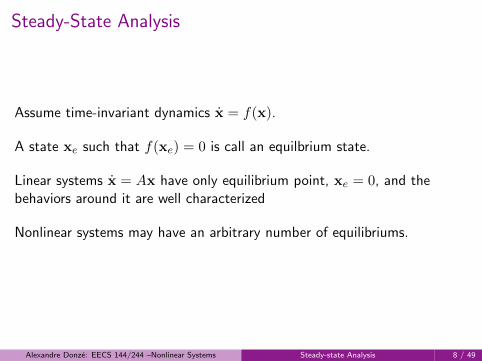
Steady-State Analysis
Assume time-invariant dynamics x = f(x).
A state xe such that f(xe) = 0 is call an equilbrium state.
Linear systems x = Ax have only equilibrium point, xe = 0, and thebehaviors around it are well characterized
Nonlinear systems may have an arbitrary number of equilibriums.
Alexandre Donze: EECS 144/244 –Nonlinear Systems Steady-state Analysis 8 / 49

Finding Steady States
To find potential equilibrium states, one has to solve the nonlinearequation:
f(x) = 0
(Note again that the fact that f is nonlinear is almost completelyirrelevant to assess the difficulty of this problem.)
Alexandre Donze: EECS 144/244 –Nonlinear Systems Steady-state Analysis 9 / 49
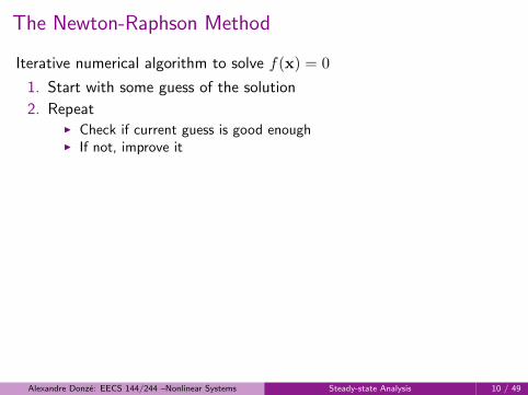
The Newton-Raphson Method
Iterative numerical algorithm to solve f(x) = 0
1. Start with some guess of the solution
2. RepeatI Check if current guess is good enoughI If not, improve it
To improve the estimate, thealgorithm make use of:
xn+1 = xn −f(xn)
f ′(xn)
Alexandre Donze: EECS 144/244 –Nonlinear Systems Steady-state Analysis 10 / 49

The Newton-Raphson Algorithm
The method generalizes to vector functions using Jacobian :
Jf (x) =
∂f1∂x1
· · · ∂f1∂xn
.... . .
...∂fn∂x1
· · · ∂fn∂xn
Start with initial guess x0, i = 0repeat
Compute jacobian Ji = Jf (xi)Let δx = J−1i f(x)Update guess xi+1 = xi + δx
until Convergence or max number iterations
Alexandre Donze: EECS 144/244 –Nonlinear Systems Steady-state Analysis 11 / 49

ConvergenceNot guaranteed :
Infinite loop
Conditions for convergence (unfortunately, no general method to enforce them):
I f has to be smooth (continuous, differentiable)
I initial guess has to be “close” to a solution
Alexandre Donze: EECS 144/244 –Nonlinear Systems Steady-state Analysis 12 / 49

Convergence rate
When it converges, quadratic.
Let f(x∗) = 0 and erri = ‖xi − x∗‖. If
1. f is smooth
2. Jf (x∗) 6= 0
3. ‖x0 − x∗‖ is small enough
Then there is a constant C such that erri+1 ≤ Cerr2i
Alexandre Donze: EECS 144/244 –Nonlinear Systems Steady-state Analysis 13 / 49

Stopping criterions
I On xi using relative and absolute tolerances :
Stops when ‖xi+1 − xi‖ ≤ εabs + εrel‖xi‖
I or on the residual ‖f(xi)‖.
Stops when ‖f(xi)‖ ≤ εabs
I or some combination... Ultimately, specific tuning to your function
Note
I εrel is typically between 10−3 and 10−6
I εabs between 10−9 and 10−12 or small with respect to typical values of x
I This applies to tolerances for ODE solver as well
Alexandre Donze: EECS 144/244 –Nonlinear Systems Steady-state Analysis 14 / 49

Linearization
Once an equilibrium state has been found, one can study locally the behavior ofthe system
x = F (xe) +∂F
∂x
∣∣∣∣xe
(x− xe) + higher order terms in (x− xe).
More generally, the system
x = f(x,u) x ∈ Rn,u ∈ Ry = h(x,u) y ∈ R
can be linearized about an equibrium point x = xe,u = ue,y = ye, by definingnew variables:
z = x− xe v = u− ue w = y − h(xe,ue)
Alexandre Donze: EECS 144/244 –Nonlinear Systems Steady-state Analysis 15 / 49

Linearization (cont’d)
The dynamics of the system near the equilibrium point can then beapproximated by the linear system
x = Ax+Bu
y = Cx+Du
where
A =∂f(x,u)
∂x
∣∣∣∣xe,ue
B =∂f(x,u)
∂u
∣∣∣∣xe,ue
C =∂h(x,u)
∂x
∣∣∣∣xe,ue
D =∂y(x,u)
∂u
∣∣∣∣xe,ue
Alexandre Donze: EECS 144/244 –Nonlinear Systems Steady-state Analysis 16 / 49

Stability Analysis
An equilibrium point is (locally) stable if initial conditions that start nearan equilibrium point stay near that equilibrium point.
A equilibrium point is (locally) asymptotically stable if it is stable and thestate of the system converges to the equilibrium point as time increases.
Note
I Stability for nonlinear systems is a local property
I Depending on initial conditions, the system can converge to differentequilibriums (see “Bi-stability”, regions of attraction, etc)
Alexandre Donze: EECS 144/244 –Nonlinear Systems Steady-state Analysis 17 / 49

Lyapunov Stability
A Lyapunov function is an energy-like function V : Rn → R that can beused to reason about the stability of an equilibrium point.
We define the derivative of V along the trajectory of the system as
V (x) =∂V
∂xx =
∂V
∂xf(x)
Assuming xe = 0 and V (0) = 0
Condition on V Condition on V Stability
V (x) > 0, x 6= 0 V (x) ≤ 0 for all x xe is stable
V (x) > 0, x 6= 0 V (x) < 0, x 6= 0 xe is asymptotically stable
Finding a Lyapunov function is a difficult problem in general - systematicmethod exist mostly for linear systems.
Alexandre Donze: EECS 144/244 –Nonlinear Systems Steady-state Analysis 18 / 49

1 Definitions (?)
2 Steady-state Analysis
3 Temporal Logics for Continuous SystemsSignal Temporal LogicQuantitative Semantics of STL
4 ApplicationsVoltage Controlled OscillatorSystems Biology
Alexandre Donze: EECS 144/244 –Nonlinear Systems Temporal Logics for Continuous Systems 19 / 49

Idea: characterizing behaviors of dynamical systems in a formalized way
In the following, I will be using Breach, a matlab toolbox available at
www.eecs.berkeley.edu/~donze/breach_page.html
It allows to (among other things)
I Simulate ODEs and Simulink systems
I Define Signal Temporal Logic properties
I Verify them on simulations results
Alexandre Donze: EECS 144/244 –Nonlinear Systems Temporal Logics for Continuous Systems 20 / 49

Outline
1 Definitions (?)
2 Steady-state Analysis
3 Temporal Logics for Continuous SystemsSignal Temporal LogicQuantitative Semantics of STL
4 ApplicationsVoltage Controlled OscillatorSystems Biology
Alexandre Donze: EECS 144/244 –Nonlinear Systems Temporal Logics for Continuous Systems 21 / 49

Outline
1 Definitions (?)
2 Steady-state Analysis
3 Temporal Logics for Continuous SystemsSignal Temporal LogicQuantitative Semantics of STL
4 ApplicationsVoltage Controlled OscillatorSystems Biology
Alexandre Donze: EECS 144/244 –Nonlinear Systems Temporal Logics for Continuous Systems 21 / 49

Temporal logics in a nutshell
Temporal logics allow to specify patterns that timed behaviors of systems may ormay not satisfy. They come in many flavors.
One of the most common is Linear Temporal Logic (LTL), dealing with discretesequences of states.
Based on logic operators (¬, ∧, ∨) and temporal operators: “next”, “always”(�), “eventually” (♦) and “until” ( U )
Examples:
I ϕ ϕ ϕ ϕ · · · satisfies � ϕ
I ψ ψ ψ ϕ ψ · · · satisfies ♦ ϕ
I ϕ ϕ ϕ ϕ ψ · · · satisfies ϕ U ψ
Alexandre Donze: EECS 144/244 –Nonlinear Systems Temporal Logics for Continuous Systems 22 / 49

From Discrete to Continuous
Temporal logics developed for discrete systems
Why not discretize time and space and reuse existing logics and tools ?
Some reasons:
I A priori arbitrary discretization often leads either to state-explosion ortoo coarse approximation
I Specifications should not depend on the discretization used (e.g.,“next” depends on time step)
Thus we need:
I Temporal specifications involving dense-time intervals
I Constraints applying on variable in the continuous domain
Alexandre Donze: EECS 144/244 –Nonlinear Systems Temporal Logics for Continuous Systems 23 / 49

Formal Definitions
Definition (STL Syntax)
ϕ := µ | ¬ϕ | ϕ ∧ ψ | ϕ U [a,b] ψ
where µ is a predicate of the form µ : µ(x) > 0
Definition (STL Semantics)
The validity of a formula ϕ with respect to a signal x at time t is
(x, t) |= µ ⇔ µ(x[t]) > 0(x, t) |= ϕ ∧ ψ ⇔ (x, t) |= ϕ ∧ (x, t) |= ψ(x, t) |= ¬ϕ ⇔ ¬((x, t) |= ϕ)(x, t) |= ϕ U[a,b] ψ ⇔ ∃t′ ∈ [t+ a, t+ b] s.t. (x, t′) |= ψ ∧
∀t′′ ∈ [t, t′], (x, t′′) |= ϕ}
Additionally: ♦[a,b]ϕ = > U[a,b] ϕ and �[a,b]ϕ = ϕ U[a,b] ⊥.
Alexandre Donze: EECS 144/244 –Nonlinear Systems Temporal Logics for Continuous Systems 24 / 49

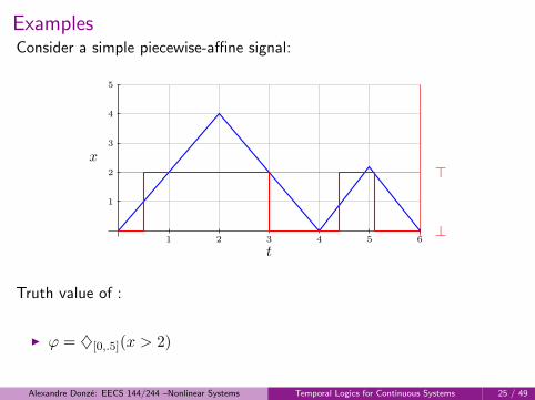
ExamplesConsider a simple piecewise-affine signal:
x
t
>
⊥1 2 3 4 5 6
1
2
3
4
5
Truth value of :
I ϕ = x > 2
II ϕ = �[0.5,1.5](x > 2)
Alexandre Donze: EECS 144/244 –Nonlinear Systems Temporal Logics for Continuous Systems 25 / 49

ExamplesConsider a simple piecewise-affine signal:
x
t
>
⊥1 2 3 4 5 6
1
2
3
4
5
Truth value of :
I ϕ = x > 2
II ϕ = �[0.5,1.5](x > 2)
Alexandre Donze: EECS 144/244 –Nonlinear Systems Temporal Logics for Continuous Systems 25 / 49

ExamplesConsider a simple piecewise-affine signal:
x
t
>
⊥1 2 3 4 5 6
1
2
3
4
5
Truth value of :
I ϕ = x > 2
I ϕ = ♦[0,∞](x > 2)
I ϕ = �[0.5,1.5](x > 2)
Alexandre Donze: EECS 144/244 –Nonlinear Systems Temporal Logics for Continuous Systems 25 / 49
ExamplesConsider a simple piecewise-affine signal:
x
t
>
⊥1 2 3 4 5 6
1
2
3
4
5
Truth value of :
I ϕ = x > 2
I ϕ = ♦[0,.5](x > 2)
I ϕ = �[0.5,1.5](x > 2)
Alexandre Donze: EECS 144/244 –Nonlinear Systems Temporal Logics for Continuous Systems 25 / 49

ExamplesConsider a simple piecewise-affine signal:
x
t
>
⊥1 2 3 4 5 6
1
2
3
4
5
Truth value of :
I ϕ = x > 2
II ϕ = �[0,∞](x > 2)
ϕ = �[0.5,1.5](x > 2)
Alexandre Donze: EECS 144/244 –Nonlinear Systems Temporal Logics for Continuous Systems 25 / 49

ExamplesConsider a simple piecewise-affine signal:
x
t
>
⊥1 2 3 4 5 6
1
2
3
4
5
Truth value of :
I ϕ = x > 2
II ϕ = �[0.5,1.5](x > 2)
Alexandre Donze: EECS 144/244 –Nonlinear Systems Temporal Logics for Continuous Systems 25 / 49
Outline
1 Definitions (?)
2 Steady-state Analysis
3 Temporal Logics for Continuous SystemsSignal Temporal LogicQuantitative Semantics of STL
4 ApplicationsVoltage Controlled OscillatorSystems Biology
Alexandre Donze: EECS 144/244 –Nonlinear Systems Temporal Logics for Continuous Systems 26 / 49

From Semantics to Satisfaction Functions
STL semantics
(x, t) � µ ⇔ µ(x[t]) > 0(x, t) � ¬ϕ ⇔ (x, t) 2 ϕ(x, t) � ϕ1 ∧ ϕ2 ⇔ (x, t) � ϕ1 and (x, t) � ϕ2
(x, t) � ϕ1 U [a,b]ϕ2 ⇔ ∃t′ ∈ [t+ a, t+ b] s.t. (x, t′) � ϕ2
and ∀t′′ ∈ [t, t′], (x, t′′) � ϕ1
A Boolean Satisfaction Function χ
Map {false, true} to {−∞,∞} and define the function χ : (x, t)→ {−∞,∞}:
χ(µ, x, t) = sign(µ(x[t]))×∞χ(¬ϕ, x, t) = − χ(ϕ, x, t)χ(ϕ1 ∧ ϕ2, x, t) = min(χ(ϕ1, x, t), χ(ϕ2, x, t))χ(ϕ1 U [a,b]ϕ2, x, t) = max
τ∈t+[a,b](min(χ(ϕ2, x, τ), min
s∈[t,τ ]χ(ϕ1, x, s))
We can verify that (x, t) |= ϕ⇔ χ(ϕ, x, t) = +∞
Alexandre Donze: EECS 144/244 –Nonlinear Systems Temporal Logics for Continuous Systems 27 / 49
From Boolean to Quantitative Satisfaction Function
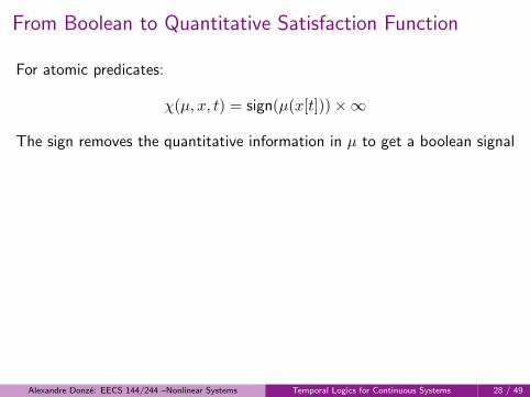
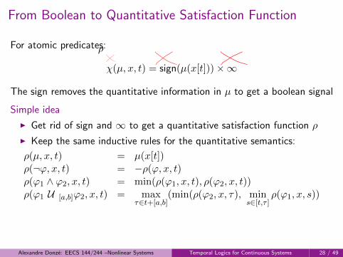
For atomic predicates:
χ(µ, x, t) = sign(µ(x[t]))×∞
The sign removes the quantitative information in µ to get a boolean signal
Simple idea
I Get rid of sign and ∞ to get a quantitative satisfaction function ρ
I Keep the same inductive rules for the quantitative semantics:
ρ(µ, x, t) = µ(x[t])ρ(¬ϕ, x, t) = −ρ(ϕ, x, t)ρ(ϕ1 ∧ ϕ2, x, t) = min(ρ(ϕ1, x, t), ρ(ϕ2, x, t))ρ(ϕ1 U [a,b]ϕ2, x, t) = max
τ∈t+[a,b](min(ρ(ϕ2, x, τ), min
s∈[t,τ ]ρ(ϕ1, x, s))
Alexandre Donze: EECS 144/244 –Nonlinear Systems Temporal Logics for Continuous Systems 28 / 49

From Boolean to Quantitative Satisfaction Function
For atomic predicates:
χ(µ, x, t) = sign(µ(x[t]))×∞
The sign removes the quantitative information in µ to get a boolean signal
Simple idea
I Get rid of sign and ∞ to get a quantitative satisfaction function ρ
I Keep the same inductive rules for the quantitative semantics:
ρ(µ, x, t) = µ(x[t])ρ(¬ϕ, x, t) = −ρ(ϕ, x, t)ρ(ϕ1 ∧ ϕ2, x, t) = min(ρ(ϕ1, x, t), ρ(ϕ2, x, t))ρ(ϕ1 U [a,b]ϕ2, x, t) = max
τ∈t+[a,b](min(ρ(ϕ2, x, τ), min
s∈[t,τ ]ρ(ϕ1, x, s))
Alexandre Donze: EECS 144/244 –Nonlinear Systems Temporal Logics for Continuous Systems 28 / 49
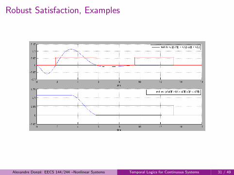
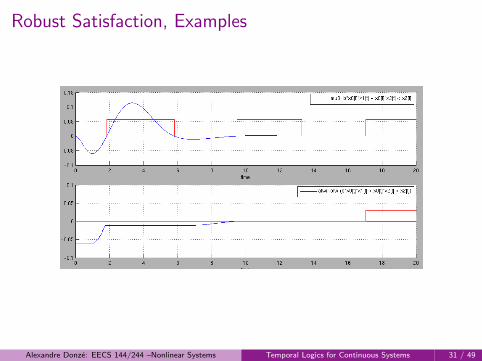
ρ
From Boolean to Quantitative Satisfaction Function
For atomic predicates:
χ(µ, x, t) = sign(µ(x[t]))×∞
The sign removes the quantitative information in µ to get a boolean signal
Simple idea
I Get rid of sign and ∞ to get a quantitative satisfaction function ρ
I Keep the same inductive rules for the quantitative semantics:
ρ(µ, x, t) = µ(x[t])ρ(¬ϕ, x, t) = −ρ(ϕ, x, t)ρ(ϕ1 ∧ ϕ2, x, t) = min(ρ(ϕ1, x, t), ρ(ϕ2, x, t))ρ(ϕ1 U [a,b]ϕ2, x, t) = max
τ∈t+[a,b](min(ρ(ϕ2, x, τ), min
s∈[t,τ ]ρ(ϕ1, x, s))
Alexandre Donze: EECS 144/244 –Nonlinear Systems Temporal Logics for Continuous Systems 28 / 49
ρ

STL operators as systems
x[t]Predicate x > 5
µ(x) = x− 5x[t]− 5
Negation ¬ϕψ(x) = −ϕ(x)
ϕ(x)[t] −ϕ(x)[t]
Conjunction ϕ1 ∧ ϕ2
ψ(x) = min(ϕ1(x), ϕ2(x))
ϕ1(x)[t]
ϕ2(x)[t]min(ϕ1(x)[t], ϕ2(x)[t])
Alexandre Donze: EECS 144/244 –Nonlinear Systems Temporal Logics for Continuous Systems 29 / 49

STL operators as systems
x[t]Predicate x > 5
µ(x) = x− 5x[t]− 5
Negation ¬ϕψ(x) = −ϕ(x)
ϕ(x)[t] −ϕ(x)[t]
Conjunction ϕ1 ∧ ϕ2
ψ(x) = min(ϕ1(x), ϕ2(x))
ϕ1(x)[t]
ϕ2(x)[t]min(ϕ1(x)[t], ϕ2(x)[t])
Alexandre Donze: EECS 144/244 –Nonlinear Systems Temporal Logics for Continuous Systems 29 / 49

STL operators as systems
x[t]Predicate x > 5
µ(x) = x− 5x[t]− 5
Negation ¬ϕψ(x) = −ϕ(x)
ϕ(x)[t] −ϕ(x)[t]
Conjunction ϕ1 ∧ ϕ2
ψ(x) = min(ϕ1(x), ϕ2(x))
ϕ1(x)[t]
ϕ2(x)[t]min(ϕ1(x)[t], ϕ2(x)[t])
Alexandre Donze: EECS 144/244 –Nonlinear Systems Temporal Logics for Continuous Systems 29 / 49

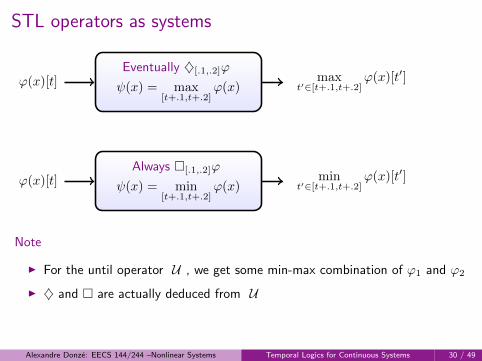
STL operators as systems
ϕ(x)[t]Eventually ♦[.1,.2]ϕ
ψ(x) = max[t+.1,t+.2]
ϕ(x)max
t′∈[t+.1,t+.2]ϕ(x)[t′]
ϕ(x)[t]Always �[.1,.2]ϕ
ψ(x) = min[t+.1,t+.2]
ϕ(x)min
t′∈[t+.1,t+.2]ϕ(x)[t′]
Note
I For the until operator U , we get some min-max combination of ϕ1 and ϕ2
I ♦ and � are actually deduced from U
Alexandre Donze: EECS 144/244 –Nonlinear Systems Temporal Logics for Continuous Systems 30 / 49

Robust Satisfaction, Examples
Alexandre Donze: EECS 144/244 –Nonlinear Systems Temporal Logics for Continuous Systems 31 / 49
Robust Satisfaction, Examples
Alexandre Donze: EECS 144/244 –Nonlinear Systems Temporal Logics for Continuous Systems 31 / 49

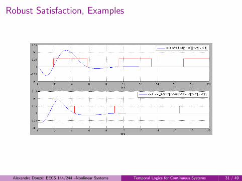
Robust Satisfaction, Examples
Alexandre Donze: EECS 144/244 –Nonlinear Systems Temporal Logics for Continuous Systems 31 / 49
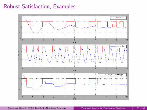
Robust Satisfaction, Examples
Alexandre Donze: EECS 144/244 –Nonlinear Systems Temporal Logics for Continuous Systems 31 / 49
Robust Satisfaction, Examples
Alexandre Donze: EECS 144/244 –Nonlinear Systems Temporal Logics for Continuous Systems 31 / 49
Robust Satisfaction, Examples
Alexandre Donze: EECS 144/244 –Nonlinear Systems Temporal Logics for Continuous Systems 31 / 49

Robust Satisfaction, Applications
Assume that x depends on p, we get the following oracle:
Param. p ∈ P
OracleModel +STL Monitor
STL Prop. ϕRobust Sat. ρ(ϕ, p)
Parameter synthesis can be solved by solving
p∗ = max {ρ(ϕ, p) | p ∈ P}
If ρ(ϕ, p∗) > 0 then parameter p∗ is such that (x, p∗) |= ϕ. Moreover, itmaximizes the robustness of satisfaction.
More generally, one can characterize the validity domain of ϕ, given byd(ϕ, P ) = {p ∈ P | ρ(ϕ, p) > 0}
Alexandre Donze: EECS 144/244 –Nonlinear Systems Temporal Logics for Continuous Systems 32 / 49

Outline
1 Definitions (?)
2 Steady-state Analysis
3 Temporal Logics for Continuous SystemsSignal Temporal LogicQuantitative Semantics of STL
4 ApplicationsVoltage Controlled OscillatorSystems Biology
Alexandre Donze: EECS 144/244 –Nonlinear Systems Applications 33 / 49
Outline
1 Definitions (?)
2 Steady-state Analysis
3 Temporal Logics for Continuous SystemsSignal Temporal LogicQuantitative Semantics of STL
4 ApplicationsVoltage Controlled OscillatorSystems Biology
Alexandre Donze: EECS 144/244 –Nonlinear Systems Applications 33 / 49
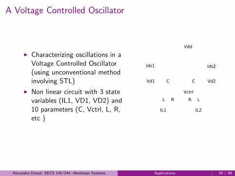
A Voltage Controlled Oscillator
I Characterizing oscillations in aVoltage Controlled Oscillator(using unconventional methodinvolving STL)
I Non linear circuit with 3 statevariables (IL1, VD1, VD2) and10 parameters (C, Vctrl, L, R,etc )
Vdd
ids1 ids2
Vd1 Vd2C C
Vctrl
IL1 IL2
L R R L
Alexandre Donze: EECS 144/244 –Nonlinear Systems Applications 34 / 49

Specifying Oscillations, Predicates
We look for oscillations of period T and given minimum and maximumamplitudes around 0
% Above and below a minimum amplitude
mu0: IL1[t] > Amin
mu1: IL1[t] < -Amin
% Bounded by a maximum amplitude
mu2: abs(IL1[t]) < Amax
% (almost) Strict periodicity
mu3: ((IL1[t] - IL1[t-T])^2 < epsi)
Alexandre Donze: EECS 144/244 –Nonlinear Systems Applications 35 / 49

Specifying Oscillations, Formulas
% Alternating above and below a minimum amplitude
phi0: (ev_[0,T] (IL1[t]>Amin)) and (ev_[0,T] (IL1[t]<-Amin))
% and holding for 4 periods
phi1: alw_[0,4*T] (phi0)
% Holding strict periodicity
phi2: alw_[0,4*T] ( (IL1[t] - IL1[t-T])^2 ) < epsi)
% Bounding amplitude globally
phi3: alw_[0,4*T] (IL1[t]^2 < Amax)
% Final formula, the ev operator gets rids of transient
phi: ev (phi1 and phi2 and phi3)
Alexandre Donze: EECS 144/244 –Nonlinear Systems Applications 36 / 49

Breach Interface
Alexandre Donze: EECS 144/244 –Nonlinear Systems Applications 37 / 49

Breach Interface
Alexandre Donze: EECS 144/244 –Nonlinear Systems Applications 37 / 49

Breach Interface
Alexandre Donze: EECS 144/244 –Nonlinear Systems Applications 37 / 49

Result on a Single Trace
Alexandre Donze: EECS 144/244 –Nonlinear Systems Applications 38 / 49

Result on a Single Trace
Alexandre Donze: EECS 144/244 –Nonlinear Systems Applications 38 / 49

Partitioning the Parameter Region
Alexandre Donze: EECS 144/244 –Nonlinear Systems Applications 39 / 49

Partitioning the Parameter Region
Alexandre Donze: EECS 144/244 –Nonlinear Systems Applications 39 / 49
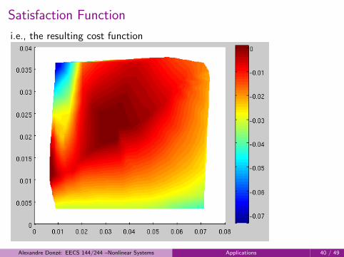
Satisfaction Function
i.e., the resulting cost function
Alexandre Donze: EECS 144/244 –Nonlinear Systems Applications 40 / 49

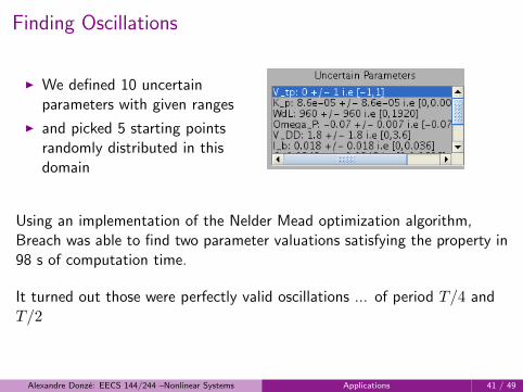
Finding Oscillations
I We defined 10 uncertainparameters with given ranges
I and picked 5 starting pointsrandomly distributed in thisdomain
Using an implementation of the Nelder Mead optimization algorithm,Breach was able to find two parameter valuations satisfying the property in98 s of computation time.
It turned out those were perfectly valid oscillations
... of period T/4 andT/2
Alexandre Donze: EECS 144/244 –Nonlinear Systems Applications 41 / 49
Finding Oscillations
I We defined 10 uncertainparameters with given ranges
I and picked 5 starting pointsrandomly distributed in thisdomain
Using an implementation of the Nelder Mead optimization algorithm,Breach was able to find two parameter valuations satisfying the property in98 s of computation time.
It turned out those were perfectly valid oscillations ... of period T/4 andT/2
Alexandre Donze: EECS 144/244 –Nonlinear Systems Applications 41 / 49

Outline
1 Definitions (?)
2 Steady-state Analysis
3 Temporal Logics for Continuous SystemsSignal Temporal LogicQuantitative Semantics of STL
4 ApplicationsVoltage Controlled OscillatorSystems Biology
Alexandre Donze: EECS 144/244 –Nonlinear Systems Applications 42 / 49

Biological networks
I Understanding a biological process through interactions between itselements
I Biological networks represents metabolism, gene regulation, signaltransduction, protein interactions, etc
genes network
proteins network
Application of formal methods
I Formalizing biological hypotheses and test them in silico
I Infer new properties and observe them in vivo
Alexandre Donze: EECS 144/244 –Nonlinear Systems Applications 43 / 49

Models for biological networks
Interaction Graphs
Petri Nets
Flux based models
Thomas networks
Differential equations,Hybrid systems
qualitative
quantitative
A number of formal methods exist for qualitative models but only a fewapply for quantitative models
STL can be used in that context
Alexandre Donze: EECS 144/244 –Nonlinear Systems Applications 44 / 49

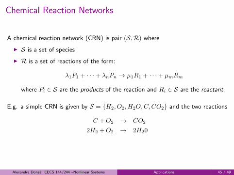
Chemical Reaction Networks
A chemical reaction network (CRN) is pair (S,R) where
I S is a set of species
I R is a set of reactions of the form:
λ1P1 + · · ·+ λnPn → µ1R1 + · · ·+ µmRm
where Pi ∈ S are the products of the reaction and Ri ∈ S are the reactant.
E.g. a simple CRN is given by S = {H2, O2, H2O,C,CO2} and the two reactions
C +O2 → CO2
2H2 +O2 → 2H20
Alexandre Donze: EECS 144/244 –Nonlinear Systems Applications 45 / 49

Mass-action kineticsGoal Given initial concentrations, predict the evolution of concentrations
The Law of Mass Action states that the rate of a reaction is proportionalto the product of the concentrations of the reactants.
In the previous example,
2H2 +O2k1−→ 2H20
C +O2k2−→ CO2
we get
d[CO2]
dt= k2[C][O2]
d[O2]
dt= − k2[C][O2]− k1[H2]
2[O2]
etc
Alexandre Donze: EECS 144/244 –Nonlinear Systems Applications 46 / 49
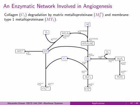
An Enzymatic Network Involved in Angiogenesis
Collagen (C1) degradation by matrix metalloproteinase (MP2 ) and membrane
type 1 metalloproteinase (MT1).
Alexandre Donze: EECS 144/244 –Nonlinear Systems Applications 47 / 49

Rigorous Steady State Analysis
In [KP04], activation of MP2 after 12h “Nearly steady state” for T2(0) between 0
and 200 nM. It turned out that steady state was not reached for T2(0) > 20 nM.
Using ϕ⇔ ♦ � (|M2(t)| < ε×MP2 (0)) we could guarantee the correct plot.
Alexandre Donze: EECS 144/244 –Nonlinear Systems Applications 48 / 49
0 20 40 60 80 100 120 140 160 180 2000
10
20
30
40
50
60
70
80
90
100
Initial concentrations of TIMP2 (nM)
% of activated MMP2
Activated MMP2 after a fixed time
12 hours

Rigorous Steady State Analysis
In [KP04], activation of MP2 after 12h “Nearly steady state” for T2(0) between 0
and 200 nM. It turned out that steady state was not reached for T2(0) > 20 nM.
Using ϕ⇔ ♦ � (|M2(t)| < ε×MP2 (0)) we could guarantee the correct plot.
Alexandre Donze: EECS 144/244 –Nonlinear Systems Applications 48 / 49
0 20 40 60 80 100 120 140 160 180 2000
10
20
30
40
50
60
70
80
90
100
Initial concentrations of TIMP2 (nM)
% of activated MMP2
Activated MMP2 after a fixed time
12 hours36 hours

Rigorous Steady State Analysis
In [KP04], activation of MP2 after 12h “Nearly steady state” for T2(0) between 0
and 200 nM. It turned out that steady state was not reached for T2(0) > 20 nM.
Using ϕ⇔ ♦ � (|M2(t)| < ε×MP2 (0)) we could guarantee the correct plot.
Alexandre Donze: EECS 144/244 –Nonlinear Systems Applications 48 / 49
0 20 40 60 80 100 120 140 160 180 2000
10
20
30
40
50
60
70
80
90
100
Initial concentrations of TIMP2 (nM)
% of activated MMP2
Activated MMP2 after a fixed time
12 hours36 hours100 hours

Rigorous Steady State Analysis
In [KP04], activation of MP2 after 12h “Nearly steady state” for T2(0) between 0
and 200 nM. It turned out that steady state was not reached for T2(0) > 20 nM.
Using ϕ⇔ ♦ � (|M2(t)| < ε×MP2 (0)) we could guarantee the correct plot.
Alexandre Donze: EECS 144/244 –Nonlinear Systems Applications 48 / 49
0 20 40 60 80 100 120 140 160 180 2000
10
20
30
40
50
60
70
80
90
100
Initial concentrations of TIMP2 (nM)
% of activated MMP2
Activated MMP2 after a fixed time
12 hours36 hours100 hoursSteady

Open ModelWe extended the model by introducing production and degradation terms
More complex behaviors becomes possible, such as oscillatory regimes
Alexandre Donze: EECS 144/244 –Nonlinear Systems Applications 49 / 49

Open ModelWe extended the model by introducing production and degradation terms
More complex behaviors becomes possible, such as oscillatory regimes
Alexandre Donze: EECS 144/244 –Nonlinear Systems Applications 49 / 49
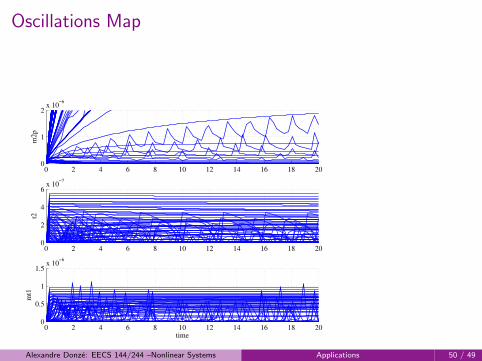
Oscillations Map
Alexandre Donze: EECS 144/244 –Nonlinear Systems Applications 50 / 49
0 2 4 6 8 10 12 14 16 18 200
1
2x 10
−6
m2
p
0 2 4 6 8 10 12 14 16 18 200
2
4
6x 10
−7
t2
0 2 4 6 8 10 12 14 16 18 200
0.5
1
1.5x 10
−6
mt1
time

Oscillations Map
Alexandre Donze: EECS 144/244 –Nonlinear Systems Applications 50 / 49
0 0.5 1 1.5 2 2.5 3
x 10−9
0
1
2
3
4
5
6x 10
−9
pm
t1
pt2
0 2 4 6 8 10 12 14 16 18 200
1
2x 10
−6
m2
p
0 2 4 6 8 10 12 14 16 18 200
2
4
6x 10
−7
t2
0 2 4 6 8 10 12 14 16 18 200
0.5
1
1.5x 10
−6
mt1
time

Oscillations Map
Alexandre Donze: EECS 144/244 –Nonlinear Systems Applications 50 / 49
0 0.5 1 1.5 2 2.5 3
x 10−9
0
1
2
3
4
5
6x 10
−9
pm
t1
pt2
0 2 4 6 8 10 12 14 16 18 200
1
2x 10
−6
m2
p
0 2 4 6 8 10 12 14 16 18 200
2
4
6x 10
−7
t2
0 2 4 6 8 10 12 14 16 18 200
0.5
1
1.5x 10
−6
mt1
time

Oscillations Map
Alexandre Donze: EECS 144/244 –Nonlinear Systems Applications 50 / 49
0 0.5 1 1.5 2 2.5 3
x 10−9
0
1
2
3
4
5
6x 10
−9
pm
t1
pt2
0 2 4 6 8 10 12 14 16 18 200
1
2x 10
−6
m2
p
0 2 4 6 8 10 12 14 16 18 200
2
4
6x 10
−7
t2
0 2 4 6 8 10 12 14 16 18 200
0.5
1
1.5x 10
−6
mt1
time