eecs349 linear discriminants - northwestern engineering · share a covariance matrix 4 g ... we...
TRANSCRIPT

Bryan Pardo, EECS 349 Machine Learning, 2013
Thanks to Mark Cartwright for his extensive contributions to these slides Thanks to Alpaydin, Bishop, and Duda/Hart/Stork for images and ideas
Machine Learning
Topic 5: Linear Discriminants
1

There is a set of possible examples Each example is an k-tuple of attribute values
There is a target function that maps X onto some finite set Y The DATA is a set of tuples <example, target function values>
Find a hypothesis h such that...
General Classification Learning Task
},...{ 1 nxxX !!=
>=< kaax ,...,11!
YXf →:
})(,,...)(,{ 11 ><><= mm xfxxfxD !!!!
)()(, xfxhx !!! ≈∀Bryan Pardo, Machine Learning: EECS 349
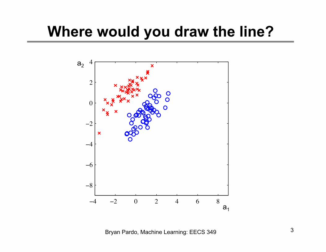
Where would you draw the line?
3
ï� ï� 0 � � 6 8
ï�
ï�
ï�
ï�
0
�
�a2
a1
Bryan Pardo, Machine Learning: EECS 349
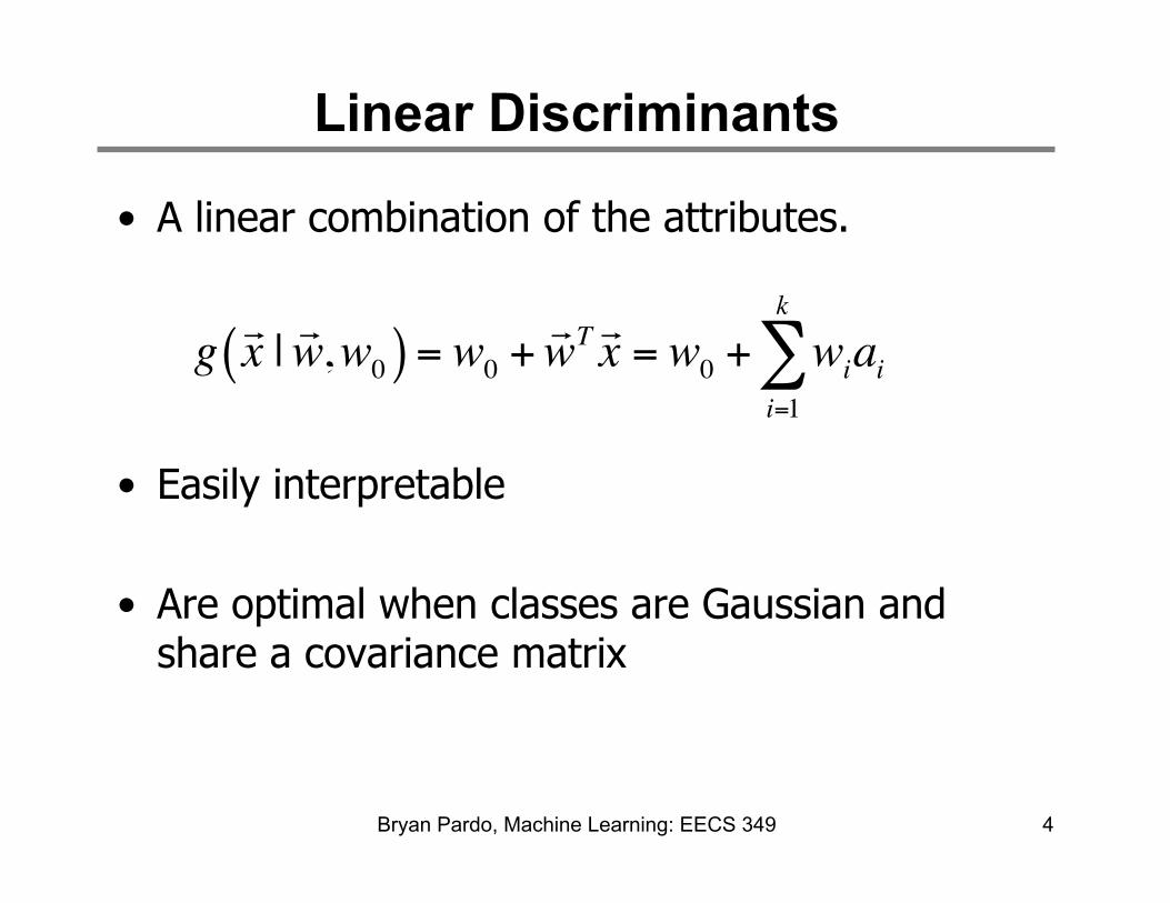
Linear Discriminants
• A linear combination of the attributes.
• Easily interpretable
• Are optimal when classes are Gaussian and share a covariance matrix
4
g x | w,w0( ) = w0 +wT x = w0 + wi
i=1
k
∑ ai
Bryan Pardo, Machine Learning: EECS 349

Two-Class Classification
5
h x( ) = 1 if g x( ) > 0
−1 otherwise
"#$
%$
defines a decision boundary that splits the space in two
g(x) = w1a1 +w2a2 +w0 = 0
g(x)> 0
g(x) = 0
a1
a2 If a line exists that does this without error, the classes are linearly separable
Bryan Pardo, Machine Learning: EECS 349
g(x)< 0
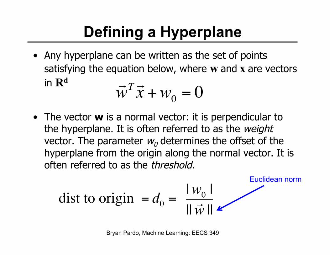
• Any hyperplane can be written as the set of points satisfying the equation below, where w and x are vectors in Rd
• The vector w is a normal vector: it is perpendicular to the hyperplane. It is often referred to as the weight vector. The parameter w0 determines the offset of the hyperplane from the origin along the normal vector. It is often referred to as the threshold.
Defining a Hyperplane
wT x +w0 = 0
dist to origin = d0 = |w0 ||| w ||
Euclidean norm
Bryan Pardo, Machine Learning: EECS 349

Estimating the model parameters
There are many ways to estimate the model parameters: • Minimize least squares criteria (classification via
regression)
• Maximize Fisher linear discriminant criteria
• Minimize perceptron criteria (using numerical optimization techniques, e.g. gradient descent)
• Many other methods for solving for the inequalities using constrained optimization…
7 Bryan Pardo, Machine Learning: EECS 349

Classification via regression
• Label each class by a number
• Call that the response variable
• Analytically derive a regression line
• Round the regression output to the nearest label number
Bryan Pardo, Machine Learning: EECS 349 Fall 2014 8
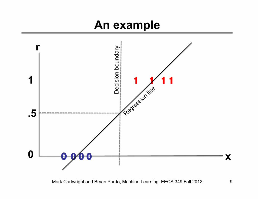
An example
Mark Cartwright and Bryan Pardo, Machine Learning: EECS 349 Fall 2012 9
0
1 1 1 1
0 O 0 0
1
.5 D
ecis
ion
boun
dary
x
r

What happens now?
Mark Cartwright and Bryan Pardo, Machine Learning: EECS 349 Fall 2012 10
0
1 1 1 1
0 O 0 0
1
.5 D
ecis
ion
boun
dary
x
r

Estimating the model parameters
There are many ways to estimate the model parameters: • Minimize least squares criteria (i.e. classification via
regression – as shown earlier)
• Maximize Fisher linear discriminant criteria
• Minimize perceptron criteria (using numerical optimization techniques, e.g. gradient descent)
• Many other methods for solving for the inequalities using constrained optimization…
11 Bryan Pardo, Machine Learning: EECS 349

Hill-climbing (aka Gradient Descent)
Obj
ectiv
e fu
nctio
n J(
w)
w: the value of some parameter
Start somewhere and head up (or down) hill.
Bryan Pardo, Machine Learning: EECS 349

Hill-climbing
Easy to get stuck in local maxima (minima)
Obj
ectiv
e fu
nctio
n J(
w)
w: the value of some parameter
Bryan Pardo, Machine Learning: EECS 349

What’s our objective function?
14 Bryan Pardo, Machine Learning: EECS 349
−1 −0.5 0 0.5 1−1
−0.5
0
0.5
1
Minimise number of misclassifications? Maximize margin between classes? Personal satisfaction?
Gradient Descent
• Simple 1st order numerical optimization method
• Idea: follow the gradient to a minimum
• Finds global minimum when objective function is convex, otherwise local minimum
• Objective function (the function you are minimizing) must be differentiable
• Used when there is no analytical solution to finding minimum
15 Bryan Pardo, Machine Learning: EECS 349
SSE: Our objective function
• We’re going to use the sum of squared errors (SSE) as our classifier error function.
• As a reminder, we used SSE in linear regression (next slide)
• Note, in linear regression, the line we learn embodies our hypothesis function. Therefore, any change in the line will change our SSE, by some amount.
Mark Cartwright and Bryan Pardo, Machine Learning: EECS 349 Fall 2012 16

Simple Linear Regression Typically estimate parameters by minimizing sum of squared residuals (a.k.a. least squares):
Mark Cartwright and Bryan Pardo, Machine Learning: EECS 349 Fall 2012 17
residual
number of training examples
Response variable
SSE: Our objective function
• In classification (next slide), the line we learn is INPUT to our hypothesis function. Therefore , a change of the line may not change the SSE objective function, if moving it does not change the classification of any training point.
• Note also, in the next slide, both the horizontal and vertical dimensions are INPUTS to the hypothesis function while in the previous slide, the vertical dimension was the OUTPUT. Therefore, the dimension a1 and a2 are the elements of the vector X that gets handed to h(x).
Mark Cartwright and Bryan Pardo, Machine Learning: EECS 349 Fall 2012 18

Simple Linear Classification Typically estimate parameters by minimizing sum of squared residuals (a.k.a. least squares):
Mark Cartwright and Bryan Pardo, Machine Learning: EECS 349 Fall 2012 19
h !x( ) = 1 if g !x( ) > 0
−1 otherwise
⎧⎨⎪
⎩⎪
E( !w) ≡ 1
2( f (!xm )
1
m
∑ − h(!xm ))2
g!x( ) = 0
a1
a2
g!x( ) > 0
g!x( ) < 0

Gradient Descent
Gradient descent is a useful, simple optimization method, but it can be very slow on difficult problems. There are many many optimization methods out there for different types of problems. Take the optimization courses offered in EECS and IEMS to learn more.
20 Bryan Pardo, Machine Learning: EECS 349
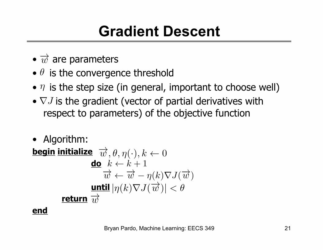
Gradient Descent
• are parameters • is the convergence threshold • is the step size (in general, important to choose well) • is the gradient (vector of partial derivatives with
respect to parameters) of the objective function
• Algorithm: begin initialize
do
until return
end
21 Bryan Pardo, Machine Learning: EECS 349

Gradient Descent
• In batch gradient descent, J is a function of both the parameters and ALL training samples, summing the total error, e.g.
• In stochastic gradient descent, J is a function of the parameters and a different single random training sample at each iteration. – this is a common choice in machine learning when there is a lot of training data, and computing the sum over all samples is expensive.
22 Bryan Pardo, Machine Learning: EECS 349

Perceptron Criteria
• Perceptron criteria:
where so that we want and is the set of misclassified training examples. • We can minimize this criteria to solve for our weight
vector w • Restricted to 2-class discriminant • We can use stochastic gradient descent to solve for this • Only converges when data is linearly separable
23
NOTE: augmented to include the threshold w0
Bryan Pardo, Machine Learning: EECS 349
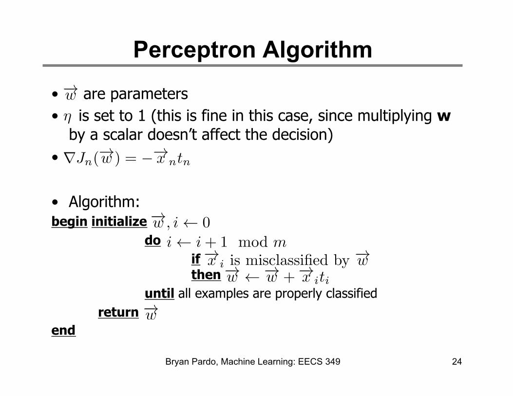
Perceptron Algorithm
• are parameters • is set to 1 (this is fine in this case, since multiplying w
by a scalar doesn’t affect the decision) •
• Algorithm: begin initialize
do if then until all examples are properly classified return
end
24 Bryan Pardo, Machine Learning: EECS 349

Perceptron Algorithm
• Example:
25
−1 −0.5 0 0.5 1−1
−0.5
0
0.5
1Red is the positive class Blue is the negative class
Bryan Pardo, Machine Learning: EECS 349
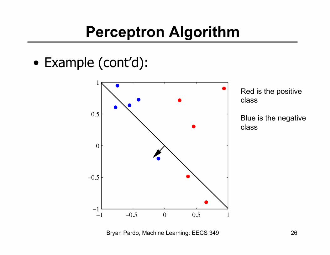
Perceptron Algorithm
• Example (cont’d):
26
−1 −0.5 0 0.5 1−1
−0.5
0
0.5
1Red is the positive class Blue is the negative class
Bryan Pardo, Machine Learning: EECS 349
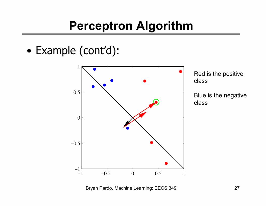
Perceptron Algorithm
• Example (cont’d):
27
−1 −0.5 0 0.5 1−1
−0.5
0
0.5
1Red is the positive class Blue is the negative class
Bryan Pardo, Machine Learning: EECS 349

Perceptron Algorithm
• Example (cont’d):
28
−1 −0.5 0 0.5 1−1
−0.5
0
0.5
1Red is the positive class Blue is the negative class
Bryan Pardo, Machine Learning: EECS 349

Multi-class Classification
29
Choose Ci if gix( ) =max
j=1
Ngjx( )
When there are N>2 classes: • you can classify using N
discriminant functions.
• Choose the class with the maximum output
• Geometrically divides feature space into N convex decision regions
a2
Bryan Pardo, Machine Learning: EECS 349
a1

Pairwise Multi-class Classification
30
If they are not linearly separable (singly connected convex regions), may still be pair-wise separable, using N(N-1)/2 linear discriminants.
gijx | wij,wij0( ) = wij0 + wijl
l=1
K
∑ xl
choose Ci if ∀j ≠ i,gij x( ) > 0
a1
a2
Bryan Pardo, Machine Learning: EECS 349

Appendix
(stuff I didn’t have time to discuss in class)
31

Fisher Linear Discriminant Criteria
• Can think of as dimensionality reduction from K-dimensions to 1
• Objective: – Maximize the difference between class means – Minimize the variance within the classes
Mark Cartwright and Bryan Pardo, Machine Learning: EECS 349 Fall 2012 32
wT x
−2 2 6
−2
0
2
4 J( w) = (m2 −m1)2
s12 + s2
2
where si and mi are thesample variance and meanfor class i in the projecteddimension. We want to maximize J.
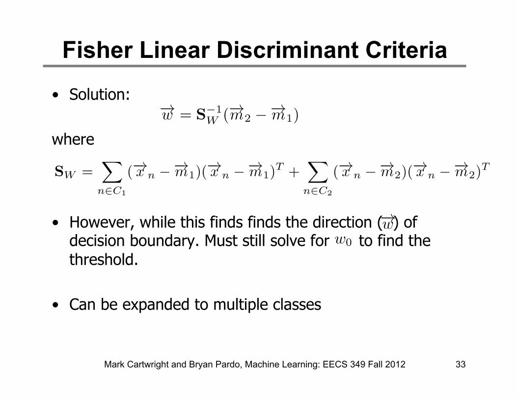
Fisher Linear Discriminant Criteria
• Solution:
where • However, while this finds finds the direction ( ) of
decision boundary. Must still solve for to find the threshold.
• Can be expanded to multiple classes
Mark Cartwright and Bryan Pardo, Machine Learning: EECS 349 Fall 2012 33

Logistic Regression (Discrimination)
Mark Cartwright and Bryan Pardo, Machine Learning: EECS 349 Fall 2012 34
0 0.5 1 1.5 2 2.5 3 3.5 40
0.5
1
1.5
2
2.5
3
3.5
4
a1
a2

Logistic Regression (Discrimination)
• Discriminant model but well-grounded in probability
• Flexible assumptions (exponential family class-conditional densities)
• Differentiable error function (“cross entropy”)
• Works very well when classes are linearly separable
Mark Cartwright and Bryan Pardo, Machine Learning: EECS 349 Fall 2012 35

Logistic Regression (Discrimination)
• Probabilistic discriminative model • Models posterior probability • To see this, let’s start with the 2-class formulation:
Mark Cartwright and Bryan Pardo, Machine Learning: EECS 349 Fall 2012 36
p(C1|x) =
p(
�!x |C1)p(C1)
p(
�!x |C1)p(C1) + p(
�!x |C2)p(C2)
=
1
1 + exp
✓� log
p(
�!x |C1)p(C1)
p(
�!x |C2)p(C2)
◆
=
1
1 + exp (�↵)
= �(↵)
where
↵ = log
p(
�!x |C1)p(C1)
p(
�!x |C2)p(C2)
1
logistic sigmoid function
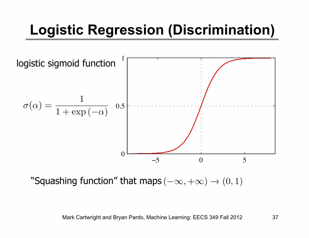
“Squashing function” that maps
Logistic Regression (Discrimination)
Mark Cartwright and Bryan Pardo, Machine Learning: EECS 349 Fall 2012 37
ï� 0 �0
���
1logistic sigmoid function

Logistic Regression (Discrimination)
Mark Cartwright and Bryan Pardo, Machine Learning: EECS 349 Fall 2012 38
For exponential family of densities, is a linear function of x. Therefore we can model the posterior probability as a logistic sigmoid acting on a linear function of the attribute vector, and simply solve for the weight vector w (e.g. treat it as a discriminant model): To classify:
p(C1|x) =
p(
�!x |C1)p(C1)
p(
�!x |C1)p(C1) + p(
�!x |C2)p(C2)
=
1
1 + exp
✓� log
p(
�!x |C1)p(C1)
p(
�!x |C2)p(C2)
◆
=
1
1 + exp (�↵)
= �(↵)
where
↵ = log
p(
�!x |C1)p(C1)
p(
�!x |C2)p(C2)
1