effective field theories - arxiv.org e-print archive¬€ective field theories 3 low energy...
TRANSCRIPT

arX
iv:h
ep-p
h/96
0622
2v1
4 J
un 1
996
Effective Field Theories
Aneesh V. Manohar
Physics Department, University of California, San Diego,9500 Gilman Drive, La Jolla, CA 92093, USA
Abstract. These lectures introduce some of the basic ideas of effective field theories.The topics discussed include: relevant and irrelevant operators and scaling, renormal-ization in effective field theories, decoupling of heavy particles, power counting, andnaive dimensional analysis. Effective Lagrangians are used to study the ∆S = 2 weakinteractions and chiral perturbation theory.
1 Introduction
An important idea that is implicit in all descriptions of physical phenomenais that of an effective theory. The basic premise of effective theories is thatdynamics at low energies (or large distances) does not depend on the detailsof the dynamics at high energies (or short distances). As a result, low energyphysics can be described using an effective Lagrangian that contains only a fewdegrees of freedom, ignoring additional degrees of freedom present at higherenergies. One of the main purposes of these lectures is to make these qualitativestatements quantitative.
First a simple example: The energy levels of the Hydrogen atom are calcu-lated in textbooks using the Schrodinger equation for an electron bound to aproton by a Coulomb potential. To a good approximation, the only propertiesof the proton that are relevant for the computation are its mass and charge.An understanding of the quark substructure of the proton (let alone quantumgravity) is not necessary to compute the energy levels of the Hydrogen states.This is true provided an answer which has some theoretical uncertainty is suf-ficient. A more accurate calculation of the energy levels, for example includingthe hyperfine splitting, requires that we also know that the proton has spin-1/2,and a magnetic moment of 2.793 nuclear magnetons. An even more accuratecalculation of the energy levels requires some knowledge of the proton chargeradius, etc. More details of the proton structure are needed as we require a moreaccurate answer for the energy levels.
When we discuss effective theories, we will frequently talk about momentumscales characteristic of a given problem. The typical length scale characteristicof the Hydrogen atom is the Bohr radius a0 = 1/(meα), and the typical mo-mentum scale is of order h/a0 ∼ 1/a0 = meα, using units in which h = 1. Thetypical energy scale characteristic of Hydrogen is the Rydberg ∼ meα
2, and thetypical time scale is 1/(meα
2). The Hydrogen atom is more complicated than
Lectures at the Schladming Winter School, March 1996, UCSD/PTH 96-04

2 Aneesh V. Manohar
many relativistic bound states because it has two characteristic scales, meα andmeα
2. We can now give a quantitative estimate of the error caused by neglectedinteractions: the energy levels of Hydrogen can be computed by ignoring all dy-namics on momentum scales Λ much larger than meα, with an error of ordermeα/Λ. As the desired accuracy increases, the scale Λ of the interactions thatcan be ignored, also increases.
The relevant interactions in an effective theory also depend on the questionbeing studied. In the Hydrogen atom, the energy levels can be computed toan accuracy (meα/MW )2 while ignoring the weak interactions, but if we areinterested in atomic parity violation, the weak interactions are the leading con-tribution since strong and electromagnetic interactions conserve parity. Atomicparity violation will still be a very small effect, because the weak scale is muchlarger than the atomic scale.
An effective field theory describes low energy physics in terms of a few pa-rameters. These low energy parameters can be computed in terms of (hopefullyfewer) parameters in a more fundamental high energy theory. This computationcan be done explicitly when the high energy theory is weakly coupled. In QED,for example, one can predict low energy parameters such as the magnetic mo-ment of the electron which can be used in the Schrodinger equation. If the highenergy theory is strong coupled, as in QCD, one usually treats the low energyparameters (such as the magnetic moment of the proton) as free parameters thatare fit to experiment. We will deal with both cases in these lectures when westudy the Fermi theory of weak interactions, and chiral perturbation theory.
We have said that high energy dynamics can be ignored in the study ofprocesses at low energies. The precise form of this statement is subtle. It is nottrue that parameters in the high energy theory do not affect the low energydynamics in any way. The precise statement is that the only effect of the highenergy theory is to modify coupling constants in the low energy theory, or to putsymmetry constraints on the low energy theory. The energy levels of Hydrogenshould not depend on the masses of heavy particles such as the top quark. Thisis not true: changing the top quark mass while keeping the electromagneticcoupling constant at high energies fixed, changes the electromagnetic couplingconstant at low energies,
mtd
dmt
(1
α
)= − 1
3π. (1)
The proton mass also depends on the top quark mass,
mp ∝ m2/27t . (2)
Despite this dependence, the value of mt is irrelevant for studying the Hydrogenatom. The reason is that α and mp are parameters of the Schrodinger equationfor the Hydrogen atom. Fitting to the observed energy levels determines the valueof α at low energies to be 1/137.036, and the proton mass to be 938.27 MeV.The value of mt is irrelevant for atomic physics if the Schrodinger equation is
treated as a low energy theory whose parameters α,me,mp are determined from

Effective Field Theories 3
low energy experiments. The value of mt is relevant if one studies how atomicphysics changes as a function of mt while keeping the high energy parametersconstant.
High energy dynamics places non-trivial symmetry constraints on a low en-ergy effective theory. An interesting example of such a constraint is the spin-statistics theorem. Non-relativistic quantum mechanics is a perfectly satisfac-tory theory, regardless of whether electrons are quantized using Bose, Fermior Boltzmann statistics. However, a consistent relativistic formulation of thetheory requires that electrons obey Fermi statistics, which is a constraint onnon-relativistic quantum mechanics that follows from causality in quantum elec-trodynamics. The spin-statistics theorem is a statement about symmetry, andholds regardless of whether there is a simple connection between the high energyand low energy theories. In low energy QCD, the spin-statistics theorem impliesthat baryons are fermions and mesons are bosons.
The effective field theory technique is powerful precisely because one cancompute low energy dynamics without any knowledge of the details of high en-ergy interactions. This also has an unfortunate consequence – information abouthigh energy interactions cannot be obtained using low energy measurements.Luckily, the last statement is not quite true. There are some vestiges of the highenergy interactions in the symmetry constraints on the low energy theory, and insmall corrections to low energy dynamics. Thus high precision low energy exper-iments can be used to probe high energy dynamics, and provide an alternativeto high energy experiments.
2 The Renormalization Group and Scaling
Effective actions were used by Wilson, Fisher, and Kadanoff to study criticalphenomena in condensed matter systems, and many of the ideas of effectivetheories were developed in this context. Consider the classic example of an Isingspin system on a square lattice with lattice spacing a, in an external magneticfield. The partition function is
Z =∑
si=±exp
K∑
〈ij〉sisj +B
∑
i
si
, (3)
where 〈ij〉 is a sum over nearest neighbors. At a second order phase transition,the correlation length ξ of the system becomes infinite. Intuitively, one expectsthat the properties of the Ising system near its critical point should not dependon the details of the system on the scale of the lattice spacing a. It took a decadeof inspired work to convert this intuitive statement into equations.
To study the Ising model at its critical point, it is not necessary to retainall the information in the partition function (3). The idea of Kadanoff was toreduce the degrees of freedom by introducing a block spin. Divide the lattice ofspins into blocks of four spins each (see Fig. 1). The block spin s′ is defined foreach block to be the average of the spins at the four corners of the block

4 Aneesh V. Manohar
s′B =sB1 + sB2 + sB3 + sB4
4, (4)
where s′B is the block spin for the block B, and sBi are the original spins at thefour corners of block B . One can write the partition function Z as
Z =∑
si=±exp
K
∑
〈ij〉sisj +B
∑
i
si
,
=
∫ ∑
si=±
∏
B
ds′Bδ
(s′B − sB1 + sB2 + sB3 + sB4
4
)
× exp
K
∑
〈ij〉sisj +B
∑
i
si
,
(5)
where the product is over all blocks B. Performing the sum over si leads to
Z =
∫ ∏
B
ds′B eS[s′B], (6)
where
eS[s′B] =
∑
si=±
∏
B
δ
(s′B − sB1 + sB2 + sB3 + sB4
4
)exp
K∑
〈ij〉sisj +B
∑
i
si
.
(7)This is an exact renormalization group transformation (called a Kadanoff blockspin transformation), that expresses the partition function in terms of a newaction S [s′B] with a quarter the number of degrees of freedom and twice thelattice spacing as the original action.
The new variable s′B is the average of four spins with values ±1 (4), and canhave the values ±1, ±1/2, 0. The new action S [s′B] is much more complicatedthan the original action K
∑〈ij〉 sisj+B
∑i si, but can in principle be computed
using (7). Now repeat the block spin transformation an infinite number of times.At each step, the number of degrees of freedom is reduced by four. The blockspin s eventually becomes a continuous variable, which is usually denoted by φ.The only problem is that the action becomes more and more complicated, andmore and more non-local at each step. This was the difficulty that prevented theKadanoff block spin method from being used for a long time. What is needed isa way to truncate the effective action in a systematic and controlled manner. Itis also important (particularly in field theory) to have an effective action that islocal.
A technical difficulty with the block spin transformation is that it is discrete;it is much easier to deal with continuous transformations. Wilson suggestedstudying the Ising model in momentum space. The variables in momentum spaceare Fourier transformed variables s(k), where the momentum k is restricted tothe Brillouin zone, |k| ≤ kmax = π/a. The Kadanoff block spin transformation

Effective Field Theories 5
/
s s
s s
B1 B2
B4 B3
sB
Fig. 1. The Kadanoff block spin transformation. The four spins at the corner of eachblock are replaced by an average spin at the center
takes a→ 2a→ 4a, etc., which corresponds to letting kmax → kmax/2 → kmax/4,etc. k is a continuous variable, so instead consider decreasing kmax continuously.The partition function transformation formula becomes (using φ,Λ instead ofs, kmax)
Z =
∫
k≤ΛDφk e−SΛ[φk] =
∫
k≤Λ′
Dφ′k e−S′
Λ′ [φ′k], (8)
which is the momentum space analog of (7). The original action SΛ [φk] containsall momentum modes up to some maximum value Λ, whereas the new actionS′Λ′ [φ′k] contains momentum modes up to Λ′, where Λ′ < Λ. The idea is to takeΛ′ = Λ−δΛ infinitesimally different from Λ, so that S′ is infinitesimally differentfrom S. In the limit δΛ→ 0, the effective action satisfies a differential equation,
∂SΛ∂Λ
= F [SΛ] , (9)
where F is a functional of the action that can be determined from (8). Thinkof SΛ as a set of actions, so that (9) gives the change in action as a function ofcutoff. This is usually referred to as the renormalization group flow of the action.The action can be written as ∑
i
ci Oi, (10)
in terms of coefficients ci and some operator basis Oi. The differential equation(9) is then a differential equation for the couplings,
∂ci∂Λ
= F [{ci}] , (11)

6 Aneesh V. Manohar
so that the renormalization group equation gives a flow in coupling constantspace.
Finally, an extremely important point: the renormalization group equationsare obtained by integrating out variables with momenta between Λ− δΛ and Λ.There is both an infrared (Λ− δΛ) and ultraviolet (Λ) cutoff on the integration,so the renormalization group equations are local and non-singular.
Free Field Theory
To explicitly study the renormalization group equations, it is helpful to considerfirst a free scalar field in D dimensions, with action
S =
∫dDx
1
2∂µφ∂
µφ− 1
2m2φ2. (12)
The action S is dimensionless, so the dimension of φ(x) is determined from thekinetic term to be [φ] = (D − 2) /2, and the dimension of m2 is
[m2]
= 2.We would like to study correlation functions
Gn (x1, . . . , xn) = 〈φ (x1) . . . φ (xn)〉S , (13)
computed using the action S at long distances (i.e. low momentum). It is con-venient to make the change of variables,
x = sx′, φ(x) = s(2−D)/2φ′(x′), (14)
so that
S′ =
∫dDx′
1
2∂′µφ
′(x′)∂′µφ′(x′) − 1
2m2s2φ′(x′)2. (15)
Correlation functions of φ(x) with action S are related to correlation func-tions of φ′(x′) with action S′ by
〈φ(sx1) . . . φ(sxn)〉S = sn(2−D)/2 〈φ′(x1) . . . φ′(xn)〉S′ . (16)
The long distance (low momentum) limit of correlation functions with action Sis obtained by letting s → ∞. These can be obtained by studying correlationfunctions at a fixed distance (fixed momentum) of the action S′ as s→ ∞. Themass term in S′ is s2m2. Clearly, in the limit s → ∞, the mass term becomesmore and more important. The mass m2 is called a relevant coupling, and dom-inates the long distance behavior of the correlation functions. Equivalently, φ2
is called a relevant operator.What about integrating out momentum shells to lower the cutoff? The orig-
inal action had an implicit cutoff Λ. We should have integrated out momentummodes and lowered the cutoff to Λ/s, so that the rescaling transformation (14)restored the cutoff to its original value Λ. In free field theory, there is no couplingbetween the different modes. Thus integrating out a momentum shell producesan overall multiplicative factor in Z, i.e. an additive constant to the effectiveaction. This shifts the cosmological constant, but does not affect the dynamicsof φ.

Effective Field Theories 7
Interactions
Next, add the interaction terms λφ4/4! + λ6φ6/6! to the free Lagrangian. The
dimensions of the coefficients are [λ] = 0, [λ6] = −2. Rescaling the field as before(and ignoring, for the moment, integrating out momenta between Λ and Λ/s)gives the rescaled action
S′ =
∫dDx′
1
2∂′µφ
′∂′µφ′ − 1
2m2s2φ′2 − λ
4!φ′4 − λ6
6!s2φ′6, (17)
with the implicit rescaled cutoff Λ. In the limit s→ ∞, the φ6 term vanishes as1/s2, so φ6 is called a irrelevant operator, and λ6 is called an irrelevant coupling.The φ4 term remains unchanged under rescaling, so it is equally important atall length scales. For this reason, φ4 is known as a marginal operator, and λ4 iscalled a marginal coupling.
In effective field theories, we are usually interested in studying the dynamicsat low energies, but not exactly at zero energy. For example, we will be studyinghadron dynamics at a scale of order 1 GeV, which is much smaller than theweak interaction scale of MW ∼ 80 GeV. In this case, the scale factor s betweenthe weak and strong scales is s = 80, which is large but finite. Irrelevant op-erators (despite their name) then produce small corrections. In our scalar fieldtheory example, the φ6 operator produces corrections of order 1/s2, φ8 producescorrections of order 1/s4, etc.
The alert reader will have noticed that the above results follow from di-mensional analysis. The counting can trivially be generalized to an arbitraryLagrangian:
1. Determine the canonical dimensions of the fields using the kinetic term.2. Determine the (mass) dimensions of all the couplings.3. Terms with a coupling constant with dimension d scale as sd, so that the
coupling is relevant, irrelevant or marginal depending on whether d > 0,d < 0 or d = 0. Equivalently, the operator is relevant, irrelevant, or marginaldepending on whether its dimension is less than, greater than, or equal tothe space-time dimension D.
4. To include all corrections up to order 1/sr, one should include all operatorswith dimension ≤ D + r, i.e. all terms with coefficients of dimension ≥ −r.
Let us now turn on the interactions. The first problem is that there are diver-gences in the quantum theory. These are handled by the standard regularizationand renormalization procedure. In scalar field theory, for example, one can in-troduce a cutoff Λ to regulate the functional integral. In the presence of a cutoff,the relation (16) between correlation functions becomes
Gn({sx} ;m2, λ4, λ6;Λ
)= sn(2−D)/2Gn
({x} ; s2m2, λ4, s
−2λ6; sΛ), (18)
where we have explicitly included the cutoff dependence, and {x} denotesx1, . . . , xn. The left hand side is the desired correlation function. To get theinfrared behavior of the left hand side, we need to replace the cutoff sΛ by Λ on

8 Aneesh V. Manohar
the right hand side. This is the hard part of the calculation which we have ignoredso far, but one that you have all seen before – it is the standard renormalizationgroup equation of quantum field theory:
[Λ∂
∂Λ+ βi
∂
∂ci+ nγφ
]G = 0. (19)
Here ci are the couplings, m2, λ, λ6, etc., and the β-functions βi and anomalousdimension γφ are functions of ci. The solution of this equation is also standard.Define running couplings which are solutions of the differential equation
Λ∂
∂Λci (Λ) = βi (ci (Λ)) . (20)
Then
Gn ({x} , ci (Λ1) , Λ1) = e−n∫Λ2
Λ1
γ(Λ)d logΛGn ({x} , ci (Λ2) , Λ2) . (21)
Equation (18) can be combined with (21) to give
G ({sx} , ci (Λ) , Λ) = sn(2−D)/2e−n∫ Λ/sΛ
γ(Λ′)d logΛ′
G({x} , sdici (Λ/s) , Λ
)
(22)where di is the dimension of coupling ci. The only difference from (16) is theexponential prefactor, and that ci is now the running coupling at Λ/s.
It is instructive to look at some examples of renormalization group equationsbefore continuing with our general analysis. In QCD, the renormalization groupequation for the dimensionless coupling constant g is
µ∂g
∂µ= − g3
16π2b0 + O
(g5), (23)
where b0 = 11Nc/3 − 2Nf/3, Nc is the number of colors, and Nf is the numberof flavors. Equation (23) is the β-function in any mass independent scheme, suchas MS, and µ is the dimensionful parameter that plays the role of Λ in such ascheme. The anomalous dimension for a field (such as the fermion field ψ) hasthe form
γψ = γ0ψ
g2
16π2+ O
(g4). (24)
Other operators added to the Lagrangian, such as four-Fermi weak decay oper-ators have renormalization group equations of the form
µ∂ci∂µ
= γ0ij
g2
16π2cj + O
(g4). (25)
Let us neglect operator mixing for simplicity, so that γij is a diagonal matrix,with elements γiδij . The solutions of the renormalization group equations are1
1 The general case where γij is not diagonal can be solved by finding the eigenvalues
and eigenvectors of γij .

Effective Field Theories 9
1
αs (µ1)− 1
αs (µ2)=b02π
logµ1
µ2,
ci (µ1)
ci (µ2)=
[αs (µ1)
αs (µ1)
]−γ0i /2b0
,
exp
[−∫ µ1
µ2
γψ (µ) d logµ
]=
[αs (µ1)
αs (µ2)
]γ0ψ/2b0
.
(26)
These equations show that the quantum scaling behavior differs from the classicalone by logarithms. A more interesting case is a field theory in which the β-function for a dimensionless coupling such as g has the form shown in Fig. 2.The renormalization group equation for g, (23), shows that g → g∗ as µ → 0if g starts out in some neighborhood of g∗. For this reason g∗ is known as anattractive (or stable) infrared fixed point for g. In this case, the renormalizationgroup scaling in the limit s→ ∞ is dominated by g ≈ g∗, so that
µ∂ci∂µ
= γij (g∗) cj ,
γφ (µ) → γφ (g∗) .
(27)
Denote the fixed point values γij (g∗) and γ (g∗) by γ∗ij and γ∗, and assume forsimplicity that γ∗ij = γ∗i δij . (As above, the general case is solved by finding theeigenvalues an eigenvectors of γ∗ij .) The solutions of the renormalization groupequations in the neighborhood of the fixed point become
ci (µ1)
ci (µ2)=
[µ1
µ2
]γ∗i
,
exp
[−∫ µ1
µ2
γφ (µ) d logµ
]=
[µ1
µ2
]−γ∗
.
(28)
so that (22) becomes
Gn ({sx} , ci (Λ) , Λ) = sn(2−D)/2snγ∗
Gn
({x} , sdi−γ∗
i ci (Λ/s) , Λ)
(29)
This equation shows that scale invariance is recovered in the quantum theory atan infrared stable fixed point, but the quantum dimensions of fields and operatorsdiffer from their classical values. Operators now have dimension D−di+γ∗i , theircoefficients have dimension di − γ∗i , and fields have dimension (D − 2) /2 − γ∗.This is the reason why γ, γij are called anomalous dimensions. The classificationinto relevant, irrelevant and marginal operators is the same as before, exceptthat one should use the quantum dimension of the operator which includes theanomalous dimension.
In weakly coupled theories, operator anomalous dimensions can be computedin perturbation theory, and are small. Thus quantum corrections cannot affectwhich operators are relevant or irrelevant, since the classical dimensions of op-erators are restricted to be integers or half-integers. The only effect of quantum

10 Aneesh V. Manohar
β(g)
g*g
Fig. 2. An infrared stable fixed point of the β function
corrections is to turn marginal operators into relevant or irrelevant operators,depending on whether their anomalous dimension is negative or positive. Instrongly coupled theories, more interesting effects can occur. For example, inwalking technicolor theories it is believed that a composite operator ψψ withclassical dimension 3 behaves in the quantum theory as a scalar field with di-mension 1, i.e. ψψ has anomalous dimension −2. A solvable example of this kindexists in two dimensions. The two dimensional Thirring model with a fundamen-tal fermion field
L = ψ(i/∂ −m
)ψ − 1
2g(ψγµψ
)2, (30)
is dual to the sine-Gordon model with a fundamental scalar field
L =1
2∂µφ∂
µφ+α
β2cosβφ, (31)
where the coupling constants g and β are related by
β2
4π=
1
1 + g/π. (32)
The fermion of the Thirring model is the sine-Gordon soliton, and the bosonof the sine-Gordon model is a fermion-antifermion bound state in the Thirringmodel. The mapping (32) shows that the strongly coupled sine-Gordon modelwith β2 ≈ 4π can be mapped onto a weakly coupled Thirring model with g ≈ 0.There are two alternate descriptions of the same theory: (a) A strongly inter-acting boson theory with large anomalous dimensions2 (b) A weakly interacting
2 For example, the operator cosβφ gets mapped to the Fermion mass term ψψ. In two
dimensions, the canonical dimensions of cos βφ and ψψ are zero and one, respectively.

Effective Field Theories 11
fermion theory with small anomalous dimensions. Formally, both descriptionsare identical, but clearly (b) is better for doing practical calculations.
The scaling dimensions of fields was determined from the free Lagrangian.That is because one assumes that the effective Lagrangian can be written as aweakly coupled field theory in terms of correctly chosen degrees of freedom at lowenergies. If the degrees of freedom are strongly coupled, the scaling dimension ofthe fields may change from their canonical value, as we saw in the sine-Gordonmodel at β2 = 4π. Often, the most difficult task in writing down an effectivetheory is choosing the right degrees of freedom. In the sine-Gordon model, it isbetter to use a weakly coupled soliton field ψ instead of the fundamental field φif β2 ≈ 4π, i.e. the effective Lagrangian for the sine-Gordon model with β2 ≈ 4πis the Thirring model. Low energy QCD is a weakly coupled theory when writtenin terms of pion fields, but not when written in terms of quark and gluon fields.1
At low energies, the Goldstone boson fields scale with canonical dimension zero(they are like angles), which is different from qq, which has dimension 3 in freefield theory. There are many examples of this kind in condensed matter physics.For example, in Landau Fermi liquid theory, the degrees of freedom are weaklyinteracting quasiparticles, not the strongly interacting electrons.
SUMMARY
We can now summarize the results of this section.
1. Find a good set of variables to describe the dynamics.
2. Write down the effective action as a sum of operators,∑
i ciOi.
3. The scaling rule is that ci → sdi−γici, where di is the naive dimension andγi is the anomalous dimension. The most important operators are those oflowest dimension. Hopefully, a good choice has been made in (1), so thatthe anomalous dimensions are small.
4. To include all corrections up to order 1/sr, one should include all operatorswith dimension ≤ D + r, i.e. all terms with coefficients of dimension ≥ −r.
There are a finite number of operators that contribute to a given order in 1/s.In four dimensions, the dimensions of scalar, spinor and vector fields is
[φ] = 1, [ψ] = 3/2, [Aµ] = 1. (33)
The allowed Lorentz invariant and gauge invariant operators of dimension ≤ 4are φn, n ≤ 4, ψψ, ∂µφ∂
µφ, ψ /Dψ, ψψφ, FµνFµν .
1 This is obvious in the large Nc limit, where one has a weakly interacting
theory of mesons and baryons, with a coupling constant 1/Nc.

12 Aneesh V. Manohar
3 Renormalizable Theories vs Effective Theories
Field theory textbooks argue that a quantum field theory should be renormaliz-able, i.e. that the Lagrangian contain only terms with dimension ≤ D. Otherwiseone needs an infinite number of counterterms, hence an infinite number of un-known parameters, and the theory has no predictive power.
An effective field theory Lagrangian contains an infinite number of terms.Let us write the Lagrangian in the form
Left = L≤D + LD+1 + LD+2 + . . . , (34)
where L≤D contains all terms with dimension ≤ D, LD+1 contains terms withdimension D + 1, LD+2 contains terms with dimension D + 2, and so on. Theusual renormalizable Lagrangian is just the first term, L≤D. There are an infi-nite number of terms in Left, but one still has approximate predictive power. Theeffective Lagrangian is used to compute processes at some scale Λ/s, where Λ isthe scale of (possibly unknown) high energy interactions. One can compute withan error of 1/s by retaining only L≤D. Furthermore, one can extend the approx-imation in a systematic way – to compute with an error of order 1/sr+1, oneneeds to retain terms up to LD+r. There are only a finite number of parametersto compute to a given order in 1/s, so the theory has predictive power.
A non-renormalizable theory is just as good as a renormalizable
theory for computations, provided one is satisfied with a finite accu-
racy.
The usual renormalizable field theory result is recovered if one takes theseparation of scales s→ ∞. In this case, one can compute using a renormalizableLagrangian L≤D with no errors. While exact computations are nice, they areirrelevant. Nobody knows the exact theory up to infinitely high energies. Thusany realistic calculation is done using an effective field theory. The standard“exact” textbook analysis of QED is really an approximate calculation in whichterms suppressed by powers of 1/s have been neglected.
4 Two Simple Examples
We now consider two simple examples that illustrates the utility of the effectivefield theory method.
Rayleigh Scattering
The first example is Rayleigh scattering, the scattering of photons off atomsat low energies. Here low energies means energies small enough that one doesnot excite the internal states of the atom, or cause it to ionize. The atom canbe treated as a particle of mass M , interacting with the electromagnetic field.Let ψ(x) denote a field operator that creates an atom at the point x. Then theeffective Lagrangian for the atom is

Effective Field Theories 13
L = ψ†(i∂t −
p2
2M
)ψ + Lint, (35)
where Lint is the interaction term. Since the atom is neutral, the interactionterm is a function of the electromagnetic field strength Fµν = (E,B). Gaugeinvariance forbids terms which depend only on the vector potential Aµ. At lowenergies, the dominant interaction is one which involves the smallest number ofderivatives, and the smallest number of photon fields, and has the form
Lint = a30 ψ
†ψ(c1E
2 + c2B2)
(36)
The electromagnetic field strength has mass dimension two, ψ has mass dimen-sion 3/2 (ψ†i∂tψ has dimension four), so that c1a
30 and c2a
30 have mass dimen-
sion −3. The typical momentum scale is set by the size of the atom a0, so oneexpects c1,2 to be of order unity. The interaction (36) gives the scattering am-plitude A ∼ cia
30ω
2, since the electric and magnetic fields are gradients of thevector potential, so each factor of E or B produces a factor of ω. The scatteringcross-section is proportional to |ci|2 a6
0ω4. This has the correct dimensions to be
a cross-section, so the phase-space is dimensionless, and one finds that
σ ∝ a60 ω
4. (37)
This reproduces the well-know ω4 dependence of the Rayleigh scattering cross-section, which explains why the sky is blue. One can actually do better, anddetermine the factors of 4π in (37), but I won’t discuss that here. Equation (37)has corrections of order ω/a0 from higher dimension operators which have beenneglected in (36).
The Euler-Heisenberg Lagrangian
The Euler-Heisenberg effective Lagrangian is the effective Lagrangian for photon-photon scattering at energies much lower than the electron massme. The leadingorder Lagrangian is the free Maxwell theory,
L = −1
4FµνF
µν . (38)
The first interactions that can occur are from higher dimension operators. Thelowest non-trivial operators must contain four factors of the field strength Fµνand hence must be of dimension eight,
L =α2
m4e
[c1 (FµνF
µν)2
+ c2
(Fµν F
µν)2]. (39)
(Terms with only three field strengths are forbidden by charge conjugation sym-metry.) The effective interaction (39) is generated from the box diagram of Fig. 3.The box diagram contains four factors of the electric charge e, and one factorof 1/16π2 for the loop. In addition, the only dimensionful parameter other than

14 Aneesh V. Manohar
the external momenta is the electron mass me. This allows us to write the La-grangian in the form (39), where c1,2 are dimensionless constants. An explicitcomputation gives
c1 =1
90, c2 =
7
90. (40)
The low energy cross-section for γγ → γγ is obtained from the graph in theeffective theory, Fig. 3(b). The scattering amplitude is A ∼ α2ω4/m4
e, since eachgradient of the photon field in (39) produces one factor of ω. This produces across-section of order
σ ∼(α2ω4
m4e
)21
ω2. (41)
The phase space factor 1/ω2 is obtained using dimensional analysis. The cross-section must have dimensions of area, so the phase space must have dimension−2. The only dimensionful parameter in the effective theory is the photon energyω, so the phase space must be proportional to 1/ω2. Thus we find σ ∼ α4ω6/m8
e,with an error of order ω2/m2
e from neglected higher order interactions in (39).
(a) (b)
Fig. 3. Light by light scattering in (a) QED and (b) in the Euler-Heisenberg effec-tive theory. The solid dot represents the four-photon interaction from the effectiveLagrangian (39)
5 Weak Interactions at Low Energies: Tree Level
The classic example of an effective field theory is the Fermi theory of weakinteractions. We first discuss how to obtain the Fermi theory as the low-energylimit of the renormalizable SU(2) × U(1) electroweak theory at tree level. Theuse of effective field theories for the tree level weak interactions will seem at firstlike applying a lot of unnecessary formalism to a trivial problem; the usefulnessof the effective field theory method will only become apparent after we studythe ∆S = 2 weak interactions, which involve loop corrections in field theory.Finally, we will discuss the weak interactions including the leading logarithmicQCD corrections, for which the effective field theory method is indispensable.

Effective Field Theories 15
The basic flavor changing vertex in the quark sector is the W coupling to thequark current
− ig√2Vij qi γ
µ PL qj , (42)
where Vij is the Kobayashi-Maskawa mixing matrix, and PL = (1− γ5)/2 is theleft-handed projection operator. The lowest order ∆S = 1 amplitude arises fromsingle W exchange (Fig. 4),
A =
(ig√2
)2
VusV∗ud (uγµ PL s)
(d γν PL u
)( −igµνp2 −M2
W
), (43)
where the W boson propagator is in ’t Hooft-Feynman gauge, p is the momentumtransferred by the W , and u, d, s are quark spinors. The exchange of unphysicalscalars φ± can be neglected, since their Yukawa couplings to the light quarksare very small. The amplitude (43) produces a non-local four-quark interaction,because of the factor of p2 −M2
W in the denominator. However, if the momen-tum transfer p is small compared with MW , the non-local interaction can beapproximated by a local interaction using the Taylor series expansion
1
p2 −M2W
= − 1
M2W
(1 +
p2
M2W
+p4
M4W
+ . . .
), (44)
and retaining only a finite number of terms. To lowest order, the amplitude is
A =i
M2W
(ig√2
)2
VusV∗ud (uγµ PL s)
(d γµ PL u
)+ O
(1
M4W
). (45)
The amplitude (45) can be obtained using the effective Lagrangian
L = −4GF√2VusV
∗ud (u γµ PL s)
(d γµ PL u
)+ O
(1
M4W
), (46)
where u, d and s are now the quark fields, and we have used the definition
GF√2≡ g2
8M2W
. (47)
The effective Lagrangian (46) can be used to study the weak decays of quarksat low energies. The basic interaction is a local four-Fermion vertex, as shown inFig. 5. To avoid complications with hadronic matrix elements and QCD correc-tions (which will be discussed later), consider instead the effective Lagrangianfor µ decay
L = −4GF√2
(e γµ PL νe) (νµ γµ PL µ) + O
(1
M4W
), (48)
whose derivation is almost identical to that of (46). Using (48), neglecting the1/M4
W terms, and integrating over phase space gives the standard result for themuon lifetime at lowest order,

16 Aneesh V. Manohar
Γµ =G2Fm
5µ
192π3. (49)
This calculation is well known, and will not be repeated here.
To summarize: at lowest order, the “full theory,” which is the SU(2) × U(1)electroweak theory, can be replaced by the “effective theory,” which is QED plusthe effective Lagrangian (46) (or (48)), up to corrections of order 1/M4
W . Theeffective theory can be used to compute physical processes such as the muonlifetime. So far, the effective field theory method is a fancy way of saying thatwe have approximated the W boson propagator in Fig. 4 by 1/M2
W . The realadvantage of the effective field theory method will be apparent after we havediscussed the one-loop ∆S = 2 amplitude including QCD radiative corrections.
u
u
d
s
W
Fig. 4. W exchange diagram for the ∆S = 1 weak interactions
u
u d
s
Fig. 5. The effective four-Fermi interaction of (46). This interaction reproduces theresults of Fig. 4 to order 1/M2
W
6 Renormalization in Effective Field Theories
In quantum field theory, knowing the Lagrangian is not sufficient to compute re-sults for physical quantities. In addition, one needs to specify a way to get finite,unambiguous answers for physical quantities. In perturbation theory, this cor-responds to a choice of renormalization scheme which (i) regulates the integralsand (ii) subtracts the infinities in a systematic way. The effective Lagrangian

Effective Field Theories 17
(46) that we have constructed is non-renormalizable, since it contains an op-erator of dimension six, times a coefficient GF which is of order 1/M2
W . Theneglected 1/M4
W term contains operators of dimension eight, and so on. To usethe effective Lagrangian beyond tree level, it is necessary to give a renormaliza-tion scheme as part of the definition of the effective field theory. Without thisadditional information, the effective Lagrangian (46) is meaningless.
It is important to keep in mind that the effective field theory is a differ-
ent theory from the full theory. The full theory of the weak interactions is arenormalizable field theory. The effective field theory is a non-renormalizablefield theory, and has a different divergence structure from the full theory. Theeffective field theory is constructed to correctly reproduce the low-energy effectsof the full theory to a given order in 1/MW . The effective Lagrangian includesmore terms as one works to higher orders in 1/MW . The effective field theorymethod is useful only for computing results to a certain order in 1/MW . If oneis interested in the answer to all orders in 1/MW , it is obviously much simplerto use the full theory.
The renormalization scheme must be carefully chosen to give a sensible ef-fective field theory. To see what the possible problems might be, consider theflavor diagonal effective Lagrangian from W and Z exchange
L = −4GF√2VuiV
∗ui (uγµ PL qi) (qi γµ PL u)+(Z − exchange)+O
(1
M4W
), (50)
where i = d, s, b. At tree level, the W and Z exchange graphs contribute toflavor diagonal parity violating u-quark interactions at order GF ∼ 1/M2
W . Atone loop, the interaction (50) induces a Zuu vertex from the graph in Fig. 6which is of the form
I ∼ 1
M2W
∫d4k
1
k2, (51)
neglecting the γ-matrix structure. The 1/k2 factor is from the two fermion propa-gators in the loop, and GF has been rewritten asGF ∼ 1/M2
W . Since the effectivefield theory is valid up to energies of order MW , one can estimate the integralusing a momentum space cutoff Λ of order MW ,
I ∼ 1
M2W
Λ2 ∼ O (1) . (52)
Thus the interaction (50) produces a one loop correction to the Zuu vertex oforder one. Similarly, one can show that higher order terms, such as the dimensioneight operators, are all equally important. A loop graph of the form Fig. 6 (wherethe vertex is now a dimension eight operator) is of order
I ′ ∼ 1
M4W
∫d4k
1
k2k2 ∼ Λ4
M4W
∼ O (1) , (53)
etc. The additional k2 in the integral (53) is from the extra ∂2 at the four-quark vertex in the dimension eight operator arising from the order p2 term in

18 Aneesh V. Manohar
the expansion of (46). The loop graph with an insertion of the dimension eightoperator is just as important as the loop graph with an insertion of the dimensionsix operator; both are of order unity and cannot be neglected. Similarly, allthe higher order terms in the effective Lagrangian are equally important, andthe entire expansion breaks down. A similar problem also occurs in the flavorchanging ∆S = 1 weak interactions that we have been studying, but the analysisis more subtle because of the GIM mechanism, which is why we considered theZuu vertex.
Fig. 6. One loop correction to the Zuu vertex. The solid square represents either thedimension six four-quark interaction of eq. (50), or the dimension eight four-quarkoperator discussed in the text
The effective field theory expansion breaks down if one introduces a mass-dependent subtraction scheme such as a momentum space cutoff.3 This problemcan be cured if one uses a mass-independent subtraction scheme, such as dimen-sional regularization and minimal subtraction, in which the dimensional param-eter µ only appears in logarithms, and never as explicit powers such as µ2. Insuch a subtraction scheme β-functions and anomalous dimensions of compositeoperators are mass independent. If one estimates the integrals (51) and (53) ina mass-independent subtraction scheme, one finds
I =1
M2W
∫d4k
1
k2∼ m2
M2W
logµ,
I ′ =1
M4W
∫d4k
1
k2k2 ∼ m4
M4W
log µ,
(54)
where m is some dimensionful parameter that is not the renormalization scaleµ. It must be some other dimensionful scale that enters the loop graph of Fig. 6,such as the quark mass or the external momentum. This completely changes theestimate of the integrals. The integrals are no longer of order one, but are smallprovided m≪ MW . As a result:
3 One way to solve this problem is to use a cutoff Λ ≪ MW . This method does not
allow one to easily match between the full and effective theories, or to include QCD
corrections.

Effective Field Theories 19
1. The effective Lagrangian produces a well-defined expansion of the weak am-plitudes in powers of m/MW , where m is some low scale such as the quarkmass or the external momentum (or ΛQCD when one includes QCD effects).One has a systematic expansion in powers of some low scale over MW . Thismakes precise what is meant by neglecting 1/M4
W terms in (45).2. Loop integrals do not have a power law dependence on µ ∼MW , so one can
count powers of 1/MW directly from the effective Lagrangian. Graphs withone insertion of terms in Leff of order 1/M2
W produces amplitudes of order1/M2
W . Graphs with one insertion of terms of order 1/M4W or two insertions
of terms of order 1/M2W produce amplitudes of order 1/M4
W , etc.3. The effective field theory behaves for all practical purposes like a renormal-
izable field theory if one works to some fixed order in 1/MW . This is becausethere are only a finite number of terms in Leff that are allowed to a givenorder in 1/MW . Terms of higher order in 1/MW can be safely neglectedbecause they can never be multiplied by positive powers of MW to produceeffects comparable to lower order terms.
It is well-known that different renormalization schemes lead to equivalent an-swers for all physical quantities. In an effective field theory, a mass-independentsubtraction scheme is particularly convenient, since it provides an efficient wayof keeping only a few operators in Leff , and in deciding which Feynman graphsare important. Nevertheless, one must be able to obtain the same results in amass-dependent scheme such as a momentum space cutoff. This is true in princi-ple: a mass dependent scheme has an infinite number of contributions that are ofleading order (from the dimension four, six, eight, . . ., operators). If one resumsthis contribution, then the remaining effects (again from an infinite number ofterms) will be of order 1/M2
W . Resumming the latter leaves a contribution of1/M4
W , etc. The net result of this procedure is to reproduce the same answeras that obtained much more simply using a mass-independent renormalizationscheme. The connection between different renormalization schemes is much morecomplicated in an effective field theory (which is non-renormalizable), than in arenormalizable field theory.
7 Decoupling of Heavy Particles
There is one important drawback to using a mass-independent subtractionscheme – heavy particles do not decouple. 4 This must obviously be true sincethe contribution of particles to β-functions does not depend on the particle mass.For example, a 1 TeV charged lepton makes the same contribution as an electronto the QED β-function at 1 GeV.
It is instructive to look at the contribution of a charged fermion to the β-function in QED. Evaluating the diagram of Fig. 7 in dimensional regularizationgives
4 A mass independent subtraction scheme does not satisfy the conditions for the
Appelquist-Carazzone theorem.

20 Aneesh V. Manohar
ie2
2π2
(pµpν − p2gµν
) [ 1
6ǫ− γ
6−∫ 1
0
dx x(1 − x) logm2 − p2x(1 − x)
4πµ2
], (55)
where p is the external momentum, m is the fermion mass, γ is Euler’s constant,and µ is the scale parameter of dimensional regularization.
p p
Fig. 7. One loop contribution to the QED β-function from a fermion of mass m
Mass-Dependent Scheme
In a mass-dependent scheme, such as an off-shell momentum space subtractionscheme, one subtracts the value of the graph at a Euclidean momentum pointp2 = −M2, to get
−i e2
2π2
(pµpν − p2gµν
) [∫ 1
0
dx x(1 − x) logm2 − p2x(1 − x)
m2 +M2x(1 − x)
]. (56)
The fermion contribution to the QED β-function is obtained by acting with(e/2)Md/dM on the coefficient of i
(pµpν − p2gµν
),
β (e) = −e2M
d
dM
e2
2π2
[∫ 1
0
dx x(1 − x) logm2 − p2x(1 − x)
m2 +M2x(1 − x)
]
=e3
2π2
∫ 1
0
dx x(1 − x)M2x(1 − x)
m2 +M2x(1 − x).
(57)
The fermion contribution to the β-function is plotted in Fig. 8. When the fermionmass m is small compared with the renormalization point M , m ≪ M , the β-function contribution is
β (e) ≈ e3
2π2
∫ 1
0
dx x(1 − x) =e3
12π2. (58)
As the renormalization point passes through m, the fermion decouples, and forM ≪ m, its contribution to β vanishes as
β (e) ≈ e3
2π2
∫ 1
0
dx x(1 − x)M2x(1 − x)
m2=
e3
60π2
M2
m2. (59)
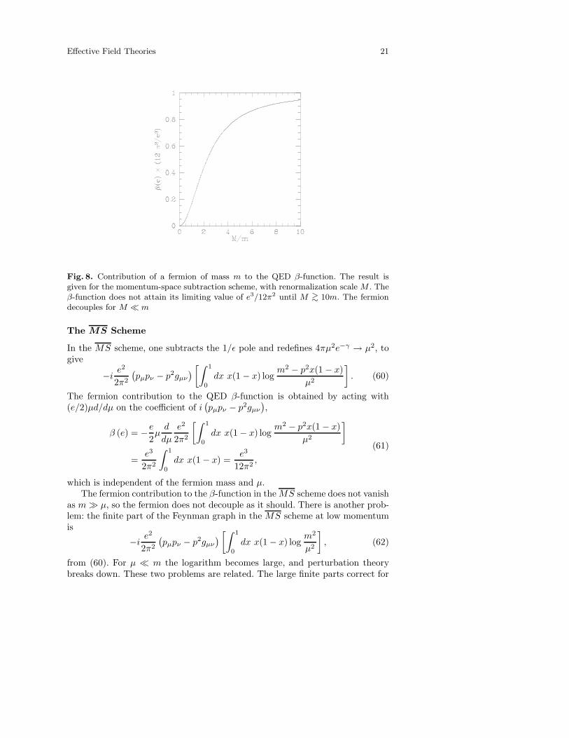
Effective Field Theories 21
Fig. 8. Contribution of a fermion of mass m to the QED β-function. The result isgiven for the momentum-space subtraction scheme, with renormalization scale M . Theβ-function does not attain its limiting value of e3/12π2 until M >
∼ 10m. The fermiondecouples for M ≪ m
The MS Scheme
In the MS scheme, one subtracts the 1/ǫ pole and redefines 4πµ2e−γ → µ2, togive
−i e2
2π2
(pµpν − p2gµν
) [∫ 1
0
dx x(1 − x) logm2 − p2x(1 − x)
µ2
]. (60)
The fermion contribution to the QED β-function is obtained by acting with(e/2)µd/dµ on the coefficient of i
(pµpν − p2gµν
),
β (e) = −e2µd
dµ
e2
2π2
[∫ 1
0
dx x(1 − x) logm2 − p2x(1 − x)
µ2
]
=e3
2π2
∫ 1
0
dx x(1 − x) =e3
12π2,
(61)
which is independent of the fermion mass and µ.The fermion contribution to the β-function in theMS scheme does not vanish
as m≫ µ, so the fermion does not decouple as it should. There is another prob-lem: the finite part of the Feynman graph in the MS scheme at low momentumis
−i e2
2π2
(pµpν − p2gµν
) [∫ 1
0
dx x(1 − x) logm2
µ2
], (62)
from (60). For µ ≪ m the logarithm becomes large, and perturbation theorybreaks down. These two problems are related. The large finite parts correct for

22 Aneesh V. Manohar
the fact that the value of the running coupling used at low energies is incorrect,because it was obtained using the “wrong” β-function. The two problems can besolved at the same time by integrating out heavy particles. One uses a theoryincluding the fermion when m < µ, and a theory without the fermion whenm > µ. Effects of the heavy particle in the low energy theory are included viahigher dimension operators, which are suppressed by inverse powers of the heavyparticle mass. The matching condition of the two theories at the scale of thefermion mass is that S-matrix elements for light particle scattering in the low-energy theory without the heavy particle must match those in the high-energytheory with the heavy particle.
For the case of a spin-1/2 fermion at one loop, this implies that the runningcoupling is continuous at m = µ. The β-function is discontinuous at m = µ,since the fermion contributes e3/12π2 to β above m and zero below m. The β-function is a step-function, instead of having a smooth crossover between e3/12π2
and zero, as in the momentum-space subtraction scheme. Decoupling of heavyparticles is implemented by hand in the MS scheme by integrating out heavyparticles at µ ∼ m. One calculates using a sequence of effective field theorieswith fewer and fewer particles. The main reason for using the MS scheme andintegrating out heavy particles is that it is much easier to use in practice than themomentum-space subtraction scheme. Virtually all radiative corrections beyondone-loop are evaluated in practice using the MS scheme.
There are some instances in which heavy particle effects are important in thelow energy effective theory. An example of this is the top quark in the standardmodel. The reason is that the top quark has a mass mt = gtv/
√2, where gt
is the top quark Yukawa coupling, and v is the vacuum expectation value ofthe Higgs field. Taking mt large while keeping v fixed is equivalent to taking gtlarge. Diagrams involving top quarks and scalars (either the Higgs boson or thelongitudinal parts of the W and Z) can be large, because they involve factorsof gt which can cancel any 1/mt suppression. We will see an example of this inthe next section, where the ∆S = 2 amplitude is shown to grow with mt. Onecan still integrate out the heavy top quark, but the low energy theory containsoperators with coefficients which grow with mt.
8 Weak Interactions at Low Energies: One Loop
The ideas discussed so far can now be applied to the weak interactions at one
loop. The amplitude for the ∆S = 2 amplitude for K0-K0
mixing is of order G2F .
The leading contribution to this amplitude in the standard model is from the boxdiagram of Fig. 9, where one sums over quarks i, j = u, c, t in the intermediatestates. The sum of the W and unphysical scalar exchange graphs is
Abox =g4
128π2M2W
∑
i,j
ξiξj E(xi, xj)(d γµ PL s
) (d γµ PL s
), (63)
where

Effective Field Theories 23
xi =m2i
M2W
, (64)
ξi = VisV∗id, (65)
E(x, y) = −xy{ 1
x− y
[1
4− 3
2
1
x− 1− 3
4
1
(x− 1)2
]log x
+1
y − x
[1
4− 3
2
1
y − 1− 3
4
1
(y − 1)2
]log y − 3
4
1
(x− 1)(y − 1)
},
(66)and
E(x, x) = −3
2
(x
x− 1
)3
log x− x
[1
4− 9
4
1
x− 1− 3
2
1
(x− 1)2
]. (67)
In the limit mu = 0 and mc,t ≪MW ,5
Abox = −G2F
4π2
(d γµ PL s
) (d γµ PL s
) [ξ2c m
2c + ξ2t m
2t + 2ξcξtm
2c log
m2t
m2c
], (68)
using (47). The ∆S = 2 amplitude is of order 1/M4W , rather than 1/M2
W asone might naively expect, because of the GIM mechanism: The quark massindependent piece of the ∆S = 2 amplitude is proportional to
ξu + ξc + ξt =∑
i
VidV∗is = 0, (69)
which vanishes because the KM matrix is unitary.
s
s
d
d
i=u,c,t
j=u,c,t
W W
Fig. 9. The box diagram for the ∆S = 2 K0−K
0
mixing amplitude
5 The ∆S = 2 amplitude is considered in the limit mt ≪ MW . This was the approxi-
mation used in the original calculations, and makes it easier for the reader to compare
with the literature. It also simplifies the discussion somewhat, because the t-quark
and c-quark can be treated in a similar fashion.

24 Aneesh V. Manohar
Matching at MW
We will now reproduce (68) using an effective field theory calculation to one loop.At the scale MW , the ∆S = 2 amplitude in the full theory is given by a loopgraph in the effective theory involving two insertions of the ∆S = 1 interaction,plus a local four-Fermi ∆S = 2 interaction. The sum of the loop graph andthe local ∆S = 2 interaction must reproduce the ∆S = 2 interaction in thefull theory to order 1/M4
W , as shown schematically in Fig. 10. The tree levelgraphs of Figs. 4 and 5 are chosen to be the same in the full and effective theoryto order 1/M2
W , but this does not imply that the loop graphs in the full andeffective theory are equal to order 1/M4
W . The two loop graphs in Fig. 10 wouldbe equal to order 1/M4
W if the loop graphs in the full and effective theory werefinite. However, in general, the graphs are infinite, and need subtractions. Thereis no simple relation between the renormalization prescriptions in the full andeffective theories and one needs to add a local ∆S = 2 counterterm at the scaleMW , which is the difference between the loop graphs in the full and effectivetheories. The graphs in the effective theory are more divergent than in the fulltheory. In our example, the box diagram in the full theory is convergent by naivepower counting.
Ifull ∼∫d4k
(1
k
)2(1
k2
)2
, (70)
whereas the graph in the effective theory is quadratically divergent,
Ieff ∼∫d4k
(1
k
)2
, (71)
where we have used a factor of 1/k for each internal fermion line, and 1/k2 foreach internal boson line. In the case of the standard model, the graph in theeffective theory is more convergent than the naive estimate because of the GIMmechanism. As we have seen, the fermion mass-independent part of the diagramis proportional to ξu + ξc + ξt, which vanishes. Thus the non-vanishing parts ofthe graphs in the full and effective theory must involve a factor of the internalfermion mass. In fact, there have to be two factors of the fermion mass becausethe ∆S = 1 vertex only involves left-handed fields, and a fermion mass changesa left-handed fermion to a right-handed fermion. Thus in the effective theory,the non-zero part of the diagram must have two mass insertions on each of thefermion lines (there is a separate GIM mechanism for each line because of theindependent sums over i and j in (63)), as represented in Fig. 10. This increasesthe degree of convergence of the diagram by two for each internal quark line,and converts it from a diagram that diverges like k2 to a diagram that convergeslike 1/k2. Since the diagrams in the full and effective theory are both finite, thelocal ∆S = 2 vertex induced at the scale MW vanishes.

Effective Field Theories 25
+=
Fig. 10. Box diagram for the ∆S = 2 amplitude in the full and effective theories. Thecrosses represent fermion mass insertions. The solid circle is a ∆S = 1 vertex, and thesolid square is a local ∆S = 2 vertex
Matching at mt
The effective Lagrangian remains unchanged down to the scale µ = mt, if oneneglects QCD radiative corrections. At the scale µ = mt, one integrates outthe top quark. The “full theory” is now the effective Lagrangian including sixquarks, and the “effective theory” is the effective Lagrangian including only fivequarks. The ∆S = 1 interactions in the five-quark theory are trivially obtainedfrom those in the six-quark theory, by dropping all terms that contain the t-quark. The ∆S = 2 interactions in the five- and six-quark theories are given inFig. 11, where the intermediate states in the six-quark theory are the u, c andt quarks, and in the five-quark theory are the u and c quarks. There is no GIMcancellation once the top quark has been integrated out of the theory, so theloop graph in the five-quark theory is divergent, and there will (in principle) bea non-zero counterterm induced at the scale mt. The value of the countertermis the difference in the diagrams in the theories above and below mt, and so isgiven by the graphs in the theory above mt that involve at least one t-quarkin the loop, as shown in Fig. 12. All other graphs in the six-quark theory areidentical to the corresponding graphs in the five-quark theory. The loop graphsin the theory above mt can be calculated quite simply, and lead to the matchingcondition
c2(µ = mt − 0) =G2F
4π2
[ξ2t m
2t + 2ξcξt
(m2t +m2
c
)+ 2ξuξt
(m2t +m2
u
)], (72)
where the contributions come from the finite part of Fig. 12, and c2 is thecoefficient of the ∆S = 2 operator
(d γµ PL s
) (d γµ PL s
). Using the relation
(69) and neglecting mu gives
c2(µ = mt − 0) =G2F
4π2
[−ξ2t m2
t + 2ξcξtm2c
]. (73)
Equation (73) is really the difference of two calculations at the scale mt
– one in the full theory and one in the effective theory. Both calculations aresensitive to infrared effects, such as confinement. However, all infrared effectscancel in the difference, and c2 (µ = mt + 0) − c2 (µ = mt − 0) is not sensitiveto infrared effects. An arbitrary infrared regulator can be used if the diagrams

26 Aneesh V. Manohar
+=u,c,t
u,c,t
u,c
u,c
Fig. 11. Matching condition at the t-quark scale. The solid square is the ∆S = 2counterterm induced at µ = mt
+ =t
t t
u,c
2
Fig. 12. Graphs to be computed to evaluate the ∆S = 2 counterterm induced atµ = mt
are infrared divergent. The loop graphs will depend on the choice of regulator,but the matching condition will not. The matching condition is only sensitive tomomenta of order µ = mt, so mass parameters such as mu are short distanceparameters such as the MS mass renormalized at µ = mt.
Scaling from mt to mc
The next step is to scale from the scale mt to mc. The loop graph Fig. 13 isdivergent, because there is no longer a GIM mechanism in the five-quark theory,and c2 is renormalized proportional to c21, where c1 is the coefficient of the∆S = 1 operator. This implies that there is a renormalization group equationfor c2,
µd
dµc2 =
1
8π2c21m
2c ξcξt, (74)
where the anomalous dimension is computed using the infinite part of Fig. 13.Integrating this equation from mt to mc gives
c2(mc) = c2(mt) +1
8π2c21 m
2c ξcξt log
mc
mt,
= c2(mt) −G2F
2π2ξcξt m
2c log
m2t
m2c
,
(75)
substituting c1 = −4GF /√
2.

Effective Field Theories 27
u,c
u,c
Fig. 13. The infinite part of this graph contributes to the renormalization group scalingof the ∆S = 2 amplitude
Matching at mc
Finally, one integrates out the c quark. This is virtually identical to the matchingcondition at the t-quark scale, and gives
c2(µ = mc − 0) = c2(µ = mc + 0) +G2F
4π2
[ξ2cm
2c + 2ξcξum
2c
]. (76)
Combining (72)–(76) reproduces the the box diagram computation (68).There are some important features of the ∆S = 2 computation which are
generic to any effective field theory computation. (i) The contributions pro-portional to the heaviest mass scale mt arise from matching conditions at thatscale. (ii) contributions proportional to lower mass scales (such as mc) arise frommatching at the scale mc, and also from from matching at scales larger than mc
(such as mt). (iii) Contributions proportional to logarithms of two scales arisefrom renormalization group evolution between the two scales.
It seems that the effective field theory method is much more complicatedthan directly computing the original box diagram in Fig. 9. The effective theorymethod has broken the computation of the box diagram into several steps. Thecomputations involved at each step in the effective field theory are much simplerthan the box diagram calculation. The box diagram involves several differentmass scales in the internal propagators, which leads to complicated Feynmanparameter integrals that must be evaluated. The matching condition computa-tions in the effective field theory each involve only a single mass scale, and aremuch simpler. One can contrast the full answer (68) with the individual piecesof the effective field theory calculation in (72)–(76). Furthermore, in the effec-tive field theory calculation it is trivial to include the leading logarithmic QCDcorrections to the ∆S = 2 amplitude. The corresponding computation in the fulltheory is far more difficult, and involves computing two loop diagrams such asthe one in Fig. 14.

28 Aneesh V. Manohar
Fig. 14. A QCD radiative correction to the box diagram
QCD Corrections
The leading logarithmic corrections to the ∆S = 2 amplitude sum all correc-tions of the form (αs log r)n, where r is large ratio of scales such as MW /mc, butneglect corrections of the form αs(αs log r)n. The QCD corrections to the match-ing condition only involve a single scale, and do not have any large logarithms.For example, the matching condition at the scale mt only involves correctionsthat depend on αs(µ) and logmt/µ. Evaluating these corrections by setting theMS parameter µ = mt implies that there is no leading logarithmic correctionto the matching condition. The only leading logarithmic QCD corrections arisefrom renormalization group scaling between different scales. This computationis straightforward, and only involves the infinite parts of one loop diagrams. Therenormalization group equation (74) is replaced by
µd
dµc2(µ) =
1
8π2m2c(µ) c21(µ) ξcξt + γ2(µ) c2(µ), (77)
where mc has been replaced by the running mass, c1 has been replaced by therunning coupling c1(µ), and γ2 is the anomalous dimension
γ2 =αs(µ)
π, (78)
of the ∆S = 2 operator (d γµ PL s) (d γµ PL s), which can be obtained from theinfinite part of Fig. 15. The running mass mc(µ) satisfies the renormalizationgroup equation
µd
dµmc(µ) = γm mc(µ) = −2αs(µ)
πmc(µ). (79)
If c1 satisfies a simple renormalization group equation of the form
µd
dµc1(µ) = γ1 c1(µ), (80)
one can solve (77)–(80) to obtain the QCD corrected value for c2(µ). At oneloop, it is convenient to define b and γi
µd
dµg = β(g) = −b g3
16π2+ . . . , (81)

Effective Field Theories 29
and
γi = γig2
16π2+ . . . , (82)
for i = 1, 2,m. One can then solve (79) and (80),
mc(µ) = mc(µ′)
[g(µ)
g(µ′)
]−γm/b=
[αs(µ
′)
αs(µ)
]γm/2b,
c1(µ) = c1(µ′)
[g(µ)
g(µ′)
]−γ1/b=
[αs(µ
′)
αs(µ)
]γ1/2b.
(83)
Substituting (83) into (77) and integrating gives
c2(mc) = c2(mt)
[αs(mt)
αs(mc)
]γ2/2b
+m2c(mt) c
21(mt)
g(mt)2 (2 + 2γ1/b+ 2γm/b− γ2/b)
[(αs(mt)
αs(mc)
)2+2γ1/b+2γm/b
−(αs(mt)
αs(mc)
)γ2/2b].
(84)
Fig. 15. Graph contributing to the anomalous dimension of the ∆s = 2 operator(d γµ PL s) (d γµ PL s)
The actual computation of these effects in the standard model is more in-volved, because the∆S = 1 Lagrangian does not satisfy a simple renormalizationgroup equation of the form (80). There is operator mixing, and (80) is replacedby a matrix equation. Nevertheless, it is possible to compute the results usingan effective field theory method, though the final form of the answer is morecomplicated than (84). The reader is referred to the papers by Gilman and Wisefor details. The computation of QCD corrections in the full theory is far morecomplicated, and has never been done.
To compare the advantages and disadvantages of the full and effective theorycomputation, let us concentrate only on the mt part of the ∆S = 2 amplitude.The effective field theory computation gives the ∆S = 2 amplitude as an expan-sion in powers of mt/MW , and we have computed the leading term in (68). Thegeneral form of the effective field theory result is

30 Aneesh V. Manohar
answer =
(mt
MW
)2(αs(MW )
αs(mt)
)γ2/2b+
(mt
MW
)4(αs(MW )
αs(mt)
)γ4/2b+ . . . (85)
where γi are the anomalous dimensions of the dimension six, eight, etc. operators.(For example, compare with (84).) Evaluating each of these anomalous dimensionis a separate computation. Equation (85) is useful if there is a large ratio of scales,mt/MW ≪ 1, so that one only needs a few terms in the expansion (85). The fulltheory computation (63) sums up the entire series, and gives an answer of theform
answer = f(mt/MW ), (86)
which is valid for any value of the ratio mt/MW . The computations involved in(86) are necessarily more complicated than those for the effective field theory,because one obtains the entire functional form of the answer, rather than the firstfew terms in a series expansion. However, it is not possible to compute the leadinglogarithmic QCD corrections to (86), since each term in the expansion has adifferent anomalous dimension. For the c quark, it is more important to sum theleading QCD corrections, than to include higher order terms in mc/MW ∼ 1/50,and the effective theory method is useful. The recently measured value of thetop quark mass indicates that the ratio mt/MW ∼ 2. In this case, it is moreimportant to retain the entire form of the mt/MW dependence, than to includethe QCD radiative corrections. The way the calculation is done in practice isto integrate out the t-quark and W -boson together at some scale µ which iscomparable to both mt and MW , and then use an effective theory to scale downto mc so as to include the QCD corrections between {MW ,mt} and mc. Clearly,the ideal procedure would be to retain the entire functional form (86), as well asthe entire QCD radiative correction. This has been done in a toy model using anon-local effective Lagrangian, but it is not known how to do this in general.
A very different example where an infinite set of anomalous dimensions canbe computed is the QCD evolution of parton structure functions. In QCD, theAltarelli-Parisi splitting functions for the parton distribution functions containthe same information as the infinite set of anomalous dimensions of the twist-two operators. The distribution functions can be written as matrix elementsof non-local operators, and the one-loop anomalous dimension is a function,whose moments give the anomalous dimensions of the infinite tower of twist twooperators.
9 The Non-linear Sigma Model
The previous results discussed effective field theories in the perturbative regime,where one could compute the effective Lagrangian from the full theory in asystematic perturbative expansion. One can also apply effective field theory ideasto situations where one can not derive the effective Lagrangian from the fulltheory directly. The classic example of this is the use of non-linear sigma modelsto study spontaneously broken global symmetries, and in particular, the use ofchiral Lagrangians to study pion interactions in QCD.

Effective Field Theories 31
Consider first the linear sigma model with Lagrangian
L = 12∂µφφ · ∂µφφ− λ(φφ · φφ− v2)2, (87)
where φφ = (φ1, . . . , φN ) is a real N -component scalar field. This theory willillustrate some ideas which will be needed for the study of chiral symmetrybreaking in QCD. The Lagrangian (87) has a global O(N) symmetry underwhich φφ transforms as an O(N) vector. The potential has been chosen so thatit is minimized for |φφ| = v. The set of field configurations where |φφ| = v isknown as the vacuum manifold, and in our example, it is the set of pointsφφ = (φ1, . . . , φN ), with φ2
1 + φ22 + . . .+ φ2
N = v2, i.e. it is the N − 1 dimensionalsphere SN−1. The O(N) symmetry can be used to rotate the vector 〈φφ〉 toa standard direction, which can be chosen to be (0, 0, . . . , v), the north poleof the sphere. The vacuum of the Lagrangian has spontaneously broken theO(N) symmetry down to the O(N − 1) subgroup which acts on the first N − 1components. The other generators of O(N) do not leave (0, 0, . . . , v) invariant.O(N) has N(N − 1)/2 generators, so the number of Goldstone bosons is equalto the number of broken generators, N(N − 1)/2 − (N − 1)(N − 2)/2 = N − 1.The N − 1 Goldstone bosons correspond to rotations of the vector φφ, whichleave its length unchanged. The potential energy V is unchanged under rotationsof φφ, so these modes are massless. The remaining mode is a radial excitationwhich changes the length of φφ, and produces a massive excitation, with massmH =
√8λ v.
It is convenient to switch to “polar coordinates”, and define
φφ = (ρ+ v) ei∑
sXs·πs
00...1
, (88)
where Xs, s = 1, . . . , N − 1 are N − 1 broken generators, and πs and ρ are anew basis for the N fields. This change of variables is only well-defined for smallangles πs. The Lagrangian in terms of the new fields is
L =1
2∂µρ∂
µρ− λ(ρ2 + 2ρv
)2+
1
2(ρ+ v)
2[∂µe
−i∑
sXs·πs∂µei
∑sXs·πs
]
NN,
(89)where [ ]NN is the NN element of the matrix. At energies small compared to theradial excitation mass
√8λ v, the ρ field can be neglected, and the Lagrangian
reduces to
L =1
2v2[∂µe
−i∑
sXs·πs∂µei
∑sXs·πs
]
NN, (90)
which describes the self-interactions of the Goldstone bosons.There are some generic features of Goldstone boson interactions that are easy
to understand:

32 Aneesh V. Manohar
1. The Goldstone boson fields are derivatively coupled. The Goldstone bosonsdescribe the local orientation of the φφ field. A constant Goldstone bosonfield is a φφ field that has been rotated by the same angle everywhere inspacetime, and corresponds to a vacuum that is equivalent to the standardvacuum 〈φφ〉 = (0, 0, . . . , 1). Thus the Lagrangian must be independent of πs
when πs is a constant, so only gradients of πs appear in the Lagrangian.2. The effective Lagrangian describes a theory of weakly interacting Goldstone
bosons at low energy. The Goldstone boson couplings are proportional totheir momentum, and so vanish for low-momentum Goldstone bosons.
3. The Goldstone boson Lagrangian is non-linear in the Goldstone bosonfields. The Goldstone boson Lagrangian describes the dynamics of fieldsconstrained to live on the vacuum manifold. The constraint equation,φ2
1 +φ22 + . . .+φ2
N = v2, is non-linear, and leads to a non-linear Lagrangian.4. The vacuum manifold is generically curved (like our sphere SN−1), and does
not have a set of global coordinates. The πs coordinates defined in (88) onlymake sense for small fluctuations of the Goldstone boson fields about thenorth pole, which is adequate for perturbation theory. For studying non-perturbative effects or global properties, it is better not to introduce theangular coordinates, but to write the Lagrangian directly in terms of fieldsthat take values on the vacuum manifold, π(x) ∈ SN−1.
5. The amplitude for the broken symmetry currents to produce a Goldstoneboson from the vacuum is proportional to the symmetry breaking strengthv.
10 The CCWZ Formalism
The general formalism for effective Lagrangians for spontaneously broken sym-metries was worked out by Callan, Coleman, Wess, and Zumino. Consider a the-ory in which a global symmetry group G is spontaneously broken to a subgroupH . The vacuum manifold is the coset space G/H . In our example, G = O(N),H = O(N − 1), and G/H = O(N)/O(N − 1) = SN−1.
We would like to choose a set of coordinates which describe the local orienta-tion of the vacuum for small fluctuations about the standard vacuum configura-tion. Let Ξ(x) ∈ G be the rotation matrix that transforms the standard vacuumconfiguration to the local field configuration. The matrix Ξ is not unique: Ξh,where h ∈ H , gives the same field configuration, since the standard vacuum is in-variant under H transformations. In our example, one can describe the directionof the vector φφ by giving the O(N) matrix Ξ, where
φφ(x) = Ξ(x)
00...v
. (91)

Effective Field Theories 33
The same configuration φφ(x) can also be described by Ξ(x)h(x), where h(x) isa matrix of the form
h(x) =
(h′(x) 0
0 1
), (92)
with h′(x) an arbitrary O(N − 1) matrix, since
(h′(x) 0
0 1
)
00...v
=
00...v
. (93)
The CCWZ prescription is to pick a set of broken generators X , and choose
Ξ(x) = eiX·π(x). (94)
Consider the O(N) theory for N = 3, which is the theory of a vector φφ in three-dimensions, and so is easy to visualize. The symmetry group G is the groupG = O(3) of rotations in three-space. The standard vacuum configuration 〈φφ〉can be chosen to be φφ pointing towards the north pole N , and the unbrokensymmetry group H = O(2) = U(1) is rotations about the axis ON , where O isthe center of the sphere (see Fig. 16). The group generators are J1, J2, J3, andthe unbroken generator is J3, where Jk generate rotations about the kth axis.The CCWZ prescription is to choose
Ξ(x) = ei[J1π(x)+J2π2(x)] (95)
to represent φφ along OA. The matrix Ξ rotates a vector pointing along the ONaxis to φφ = OA by rotating along a line of longitude.
Under a global symmetry transformation g, the matrix Ξ(x) is transformedto the new matrix gΞ(x), since φφ(x) → gφφ(x). (Note that g is a global trans-formation, and does not depend on x.) The new matrix gΞ(x) is no longer instandard form, (94), but can be written as
g Ξ = Ξ ′ h, (96)
since two matrices g Ξ and Ξ ′ which describe the same field configuration dif-fer by an H transformation. That h is non-trivial is a well-known property ofrotations in three dimensions. Take an object and rotate it from N to A andthen to B. This transformation is not the same as a direct rotation from N toB, but can be written as a rotation about ON , followed by a rotation from Nto B. The transformation h in (96) is non-trivial because the Goldstone bosonmanifold G/H is curved.
The transformation (96) is usually written as
Ξ(x) → g Ξ(x) h−1(g,Ξ(x)), (97)

34 Aneesh V. Manohar
gΞ
−
NA
B
O
Ξ
Ξ
Fig. 16. The vacuum manifold for the O(3) sigma model. The standard configurationφφ is along ON . Under the transformation g, A gets mapped to B
where we have made clear the implicit dependence of h on x through its de-pendence on g and Ξ(x). Equations (94) and (97) give the CCWZ choice forthe Goldstone boson field, and its transformation law. Any other choice givesthe same results for all observables, such as the S-matrix, but does not give thesame off-shell Green functions.
11 The QCD Chiral Lagrangian
The CCWZ formalism can now be applied to QCD. In the limit that the u, dand s quark masses are neglected, the QCD Lagrangian has a SU(3)L×SU(3)Rchiral symmetry under which the left- and right-handed quark fields transformindependently,
ψL(x) → L ψL(x), ψR(x) → R ψR(x), (98)
where
ψ =
uds
. (99)
The SU(3)L × SU(3)R chiral symmetry is spontaneously broken to the vectorSU(3) subgroup by the
⟨ψψ⟩
condensate. The symmetry group is G = SU(3)L×SU(3)R, the unbroken group is H = SU(3)V , and the Goldstone boson manifoldis the coset space SU(3)L × SU(3)R/SU(3)V which is isomorphic to SU(3).The generators of G are T aL and T aR which act on left and right handed quarksrespectively, and the generators of H are the flavor generators T a = T aL + T aR.

Effective Field Theories 35
There are two commonly used bases for the QCD chiral Lagrangian, the ξ-basisand the Σ-basis, and we will consider them both. There are many simplificationsthat occur for QCD because the coset space G/H is isomorphic to a Lie group.This is not true in general; in the O(N) model, the space SN−1 is not isomorphicto a Lie group for N 6= 4.
The ξ-basis
The unbroken generators of H plus the broken generators X span the spaceof all symmetry generators of G. One choice of broken generators is to pickXa = T aL − T aR. Let the SU(3)L × SU(3)R transformation be represented inblock diagonal form,
g =
[L 00 R
], (100)
where L and R are the SU(3)L and SU(3)R transformations, respectively. Theunbroken transformation have the form (100) with L = R = U ,
h =
[U 00 U
]. (101)
The Ξ field is then defined using the CCWZ prescription (94)
Ξ(x) = eiX·π(x) = exp i
[T · π 0
0 −T · π
]=
[ξ(x) 00 ξ†(x)
], (102)
whereξ = eiT ·π (103)
denotes the upper block of Ξ(x). The transformation rule (97) gives[ξ(x) 0
0 ξ†(x)
]→[L 00 R
] [ξ(x) 00 ξ†(x)
] [U−1 0
0 U−1
]. (104)
This gives the transformation law for ξ,
ξ(x) → L ξ(x) U−1(x) = U(x) ξ(x) R†, (105)
which defines U in terms of L, R, and ξ.
The Σ basis
The Σ-basis is obtained from the CCWZ prescription using Xa = T aL for thebroken generators. In this case, (94) gives
Ξ(x) = eiX·π(x) = exp i
[T · π 0
0 0
]=
[Σ(x) 0
0 1
](106)
whereΣ = eiT ·π (107)

36 Aneesh V. Manohar
denotes the upper block of Ξ(x). The transformation law (97) is[Σ(x) 0
0 1
]→[L 00 R
] [Σ(x) 0
0 1
] [U−1 0
0 U−1
], (108)
which gives U = R, andΣ(x) → L Σ(x) R†. (109)
Comparing with (105), one sees that Σ and ξ are related by
Σ(x) = ξ2(x). (110)
The Lagrangian
The Goldstone boson fields are angular variables, and are dimensionless. Whenwriting down effective Lagrangians in field theory, it is convenient to use fieldswhich have mass dimension one, as for any other spin-zero boson field. Thestandard choice is to use
ξ = eiT ·π/f , Σ = e2iT ·π/f , (111)
where f ∼ 93 MeV is the pion decay constant. The π matrix is
ππ = πaT a, (112)
where the group generators have the usual normalization trT aT b = δab/2,
ππ =1√2
1√2π0 + 1√
6η π+ K+
π− − 1√2π0 + 1√
6η K0
K− K0 − 2√
6η
. (113)
The low energy effective Lagrangian for QCD is the most general possibleLagrangian consistent with spontaneously broken SU(3) × SU(3) symmetry.Unlike our weak interaction example, one cannot simply compute the effectiveLagrangian directly from the original QCD Lagrangian. The connection betweenthe original and effective theories is non-perturbative. The effective Lagrangianhas an infinite set of unknown parameters, but we will see that it can still beused to obtain non-trivial predictions for experimentally measured quantities.
It is easy to construct the most general Lagrangian invariant under the trans-formationΣ → LΣR†. The most general invariant term with no derivatives mustbe the product of terms of the form TrΣΣ† . . . ΣΣ†, where Σ and Σ†’s alter-nate. However, ΣΣ† = 1, so all such terms are constant, and independent of thepion fields. This is just our old result that all Goldstone bosons are derivativelycoupled. The only invariant term with two derivatives is
L2 =f2
4Tr ∂µΣ∂
µΣ†. (114)
Expanding Σ in a power series in the pion field gives

Effective Field Theories 37
L2 = Tr ∂µπ∂µπ +
1
3f2Tr [π, ∂µπ]
2+ . . . . (115)
The coefficient of the two-derivative term in (114) is fixed by requiring that thekinetic term for the pions in (115) has the standard normalization for scalarfields. The Lagrangian (114) only has terms with an even number of pions, sincethe pion is a pseudoscalar. The Lagrangian (114) determines all the multi-pionscattering amplitudes to order p2 in terms of a single constant f . For example,the π − π scattering amplitude is given by the term Tr [π, ∂µπ]
2/3f2, etc.
The Chiral Currents
Noether’s theorem can be used to compute the SU(3)L and SU(3)R currents. Ifa Lagrangian L is invariant under an infinitesimal global symmetry transforma-tion with parameter ǫ, the current jµ is given by computing the change of theLagrangian when one makes the same transformation, with ǫ a function of x,
δL = ∂µǫ(x) jµ(x). (116)
The infinitesimal form of the SU(3)L transformation Σ → LΣ is
Σ → Σ + iǫaL TaΣ, (117)
where L = exp iǫaLTa ≈ 1 + iǫaLT
a + . . .. The change in (114) under (117) is
δL = ∂µǫaL Tr T aΣ∂µΣ† (118)
so that the SU(3)L currents are
jµL =i
2f2 Tr T aΣ∂µΣ†. (119)
The right handed currents are obtained by applying the parity transformation,π(x) → −π(−x) or by making an infinitesimal SU(3)R transformation, so that
jµR =i
2f2 Tr T aΣ†∂µΣ. (120)
The axial current has the expansion
jµaA = jµaR − jµaL = −f∂µπa + . . . (121)
The matrix element 〈0| jµaA∣∣πb⟩
= ifpµδab, so that f is the pion decay constant.The experimental value of the π decay rate, π → µν determines f ≈ 93 MeV.
The low-energy effective theory of the weak interactions is an expansion insome low mass scale (such asmc or ΛQCD) overMW . The QCD chiral Lagrangianis an expansion in derivatives, and so is an expansion in p/Λχ. The pion couplingsare weak, as long as the pion momentum is small compared with Λχ. There aretwo important questions that have to be answered before one can use the effectiveLagrangian: (i) What terms in the effective Lagrangian are required to computeto a given order in p/Λχ? (ii) What is the value of Λχ? Then one has an estimate

38 Aneesh V. Manohar
of the neglected higher-order terms in the expansion, and the energy at whichthe effective theory breaks down.
It is useful to eliminate all redundant terms in the effective Lagrangian. Onecan often eliminate many terms in the effective Lagrangian by making suitablefield redefinitions. Field redefinitions are not very useful in renormalizable fieldtheories, because they make renormalizable Lagrangians look superficially non-renormalizable. For example, a field redefinition
φ→ φ+ ǫφ2, (122)
turns
L =1
2∂µφ∂
µφ− 1
2m2φ2 − λφ4 (123)
into
L =1
2∂µφ∂
µφ− 1
2m2φ2−λφ4 +ǫ
(2φ∂µφ∂
µφ−m2φ3 − 4λφ5)+O
(ǫ2), (124)
which looks superficially like a non-renormalizable interaction. Equations (124)and (123) define identical theories, and the field redefinition (122) has turneda simple Lagrangian into a more complicated one. However, in the case of non-renormalizable theories which contain an infinite number of terms, one can usefield redefinitions to eliminate many higher-order terms in the effective La-grangian (see Ref. 7). The way this is usually done in practice is to use theequations of motion derived from the lowest-order terms in the effective La-grangian to simplify or eliminate higher order terms.
Weinberg’s Power Counting Argument
The QCD chiral Lagrangian is
L =∑
k
Lk, (125)
where L2, L4, etc. are the terms in the Lagrangian with two derivatives, fourderivatives, and so on. Consider an arbitrary loop graph, such as the one inFig. 17. It contains m2 interaction vertices that come from terms in L2, m4
interaction vertices from terms in L4, etc. The general form of the diagram is
A =
∫ (d4p)L 1
(p2)I
∏
k
(pk)mk
, (126)
where L is the number of loops, I is the number of internal lines, and p representsa generic momentum. The factors are easy to understand: there is a d4p integralfor each loop, each internal boson propagator is 1/p2, and each vertex in Lk givesa factor of pk. In a mass-independent subtraction scheme, the only dimensionalparameters are the momenta p. Thus the amplitude A must have the form A ∼pD, where

Effective Field Theories 39
D = 4L− 2I +∑
k
k mk, (127)
from (126). For any Feynman graph, one can show that
V − I + L = 1, (128)
where V is the number of vertices, I is the number of internal lines, and L is thenumber of loops. Combining (127),(128), and using V =
∑kmk, one gets
D = 2 + 2L+∑
k
(k − 2)mk. (129)
The chiral Lagrangian starts at order p2, so k ≥ 2, and all terms in (129) are non-negative. As a result, only a finite number of terms in the effective Lagrangianare needed to work to a fixed order in p, and the chiral Lagrangian acts like arenormalizable field theory. For example, to compute the scattering amplitudesto order p4, one needs
4 = 2 + 2L+∑
k
(k − 2)mk, (130)
which has the solutions L = 0, m4 = 1, mk>4 = 0, or L = 1 and mk>2 = 0. Thatis, one only needs to consider tree level diagrams with one insertion of L4, orone-loop graphs with the lowest order Lagrangian L2 to compute all scatteringamplitudes to order p4.
Fig. 17. A loop graph for multipion interactions
Naive Dimensional Analysis
Consider the π − π scattering amplitude to order p4. The power counting argu-ment implies that there are two contributions to this: a tree level graph with oneinsertion of L4, and a loop graph using L2. The loop graph is of order
I ∼∫
d4k
(2π)4
k2
f2
k2
f2
1
k4, (131)

40 Aneesh V. Manohar
where 1/k4 is from the two internal propagators, and each four-pion interactionvertex is of order k2/f2, from (115). Here k denotes a generic internal momentumin the Feynman diagram. Estimating this integral gives
I ∼ p4
16π2
1
f4logµ, (132)
where µ is the MS renormalization scale, and p represents a generic externalmomentum. A four derivative operator in the Lagrangian of the form
a tr ∂µΣ∂µΣ†∂νΣ∂
νΣ†, (133)
produces a four-pion interaction of order ap4/f4 when one expands the Σ fieldin a power series in π/f . The total four-pion amplitude, which is the sum of thetree and loop graphs, is µ-independent. A shift in the renormalization scale µis compensated for by a corresponding shift in a. A change in µ of order oneproduces a shift in a of order δa ∼ 1/16π2. Generically, a must be at least asbig as δa,
|a| >∼ |δa| ∼ 1
16π2, (134)
because a shift in the renormalization point of order one produces a shift in a ofthis size. Write the effective Lagrangian as
L =f2
4
[tr ∂µΣ∂
µΣ† +1
Λ2χ
L4 +1
Λ4χ
L6 + . . .
](135)
where 1/Λχ is the expansion parameter of the effective Lagrangian, i.e. (135)gives an expansion for scattering amplitudes in powers of p/Λχ. The estimate(134) for the size of the four derivative term implies that
Λχ <∼ 4πf. (136)
One can show that a similar estimate holds for all the higher order terms inL, i.e. the six derivative term has a coefficient of order 1/Λ4
χ, etc. Numerouscalculations suggest that in QCD, the inequality (136) can be replaced by theestimate
Λχ ∼ 4πf ∼ 1 GeV, (137)
for the expansion parameter of the effective Lagrangian. This parameter is largeenough that one can apply chiral Lagrangians to low energy processes involv-ing pions and kaons. If the expansion parameter were f instead of 4πf , chiralLagrangians would not be useful even for pions, since mπ > f .
The naive dimensional analysis estimate equivalent to (135) is that a termin the Lagrangian has the form
f2Λ2χ
(π
f
)n(∂
Λχ
)m, (138)
as can be seen by expanding the (135) in the pion fields. For example, the kineticterm Tr ∂µΣ ∂µΣ† has a coefficient of order

Effective Field Theories 41
f2Λ2χ
(∂
Λχ
)2
∼ f2, (139)
the four derivative term Tr ∂µΣ ∂µΣ†∂νΣ ∂νΣ† has a coefficient of order
f2Λ2χ
(∂
Λχ
)4
∼ f2
Λ2χ
∼ 1
16π2, etc., (140)
which agrees with the earlier estimates.
12 Explicit Symmetry Breaking
The light quark masses explicitly break the chiral SU(3)L × SU(3)R symmetryof the QCD Lagrangian. The quark mass term in the QCD Lagrangian is
Lm = −ψLMψR + h.c., (141)
where
M =
mu 0 00 md 00 0 ms
, (142)
is the quark mass matrix. The mass term Lm can be treated as chirally invariantif M is an external field that transforms as
M → LMR† (143)
under chiral SU(3)L × SU(3)R. The symmetry breaking terms in the chiralLagrangian are terms that are invariant when M has the transformation rule(143). The symmetry is then explicitly broken when M is fixed to have the value(142). The lowest order term in the effective Lagrangian to first order in M is
Lm = µf2
2tr(Σ†M +M †Σ
), (144)
which breaks the degeneracy of the vacuum and picks out a particular orientationfor Σ. All vacua Σ = constant are no longer degenerate, and Σ = 1 is the lowestenergy state. Expanding in small fluctuations about Σ = 1 gives
Lm = −2µ trMπ2. (145)
Substituting (142) and (113) for M and π and evaluating the trace gives
M2π± = µ (mu +md) +∆M2,
M2K± = µ (mu +ms) +∆M2,
M2
K0,K0 = µ (md +ms) ,
(146)
and the π0, η mass matrix

42 Aneesh V. Manohar
µ
[mu +md
mu−md√3
mu−md√3
13 (mu +md + 4ms)
]. (147)
To first order in the isospin-breaking parameter mu −md, the matrix (147) haseigenvalues
M2π0 = µ (mu +md) ,
M2η =
µ
3(mu +md + 4ms) .
(148)
There is an isospin breaking electromagnetic contribution to the charged Gold-stone boson masses ∆M2 (included in (146)), which is comparable in size tothe isospin breaking from mu−md. To lowest order in SU(3) breaking, ∆M2 isequal for π± and K±, and vanishes for the neutral mesons. The absolute valuesof the quark masses can not be determined from the meson masses, because theyalways occur in the combination µm, and µ is an unknown parameter. However,the meson masses can be used to obtain quark mass ratios. From (146)–(147)one gets
mu
md=M2K+ −M2
K0 + 2M2π0 −M2
π+
M2K0 −M2
K+ +M2π+
, (149)
ms
md=M2K0 +M2
K+ −M2π+
M2K0 −M2
K+ +M2π+
, (150)
and the Gell-Mann–Okubo formula
4M2K0 = 3M2
η +M2π . (151)
Substituting the measured meson masses gives the lowest order values
mu
md= 0.55,
ms
md= 20.1. (152)
and 0.99 GeV2 = 0.92 GeV2 for the Gell-Mann–Okubo formula.There is an ambiguity in extracting the light quark masses at second order
in M . The matrices M and (detM)M †−1 both have the same SU(3)L×SU(3)Rtransformation properties, and are indistinguishable in the chiral Lagrangian.One has an ambiguity of the form
M →M + λ (detM)M †−1 (153)
in the quark mass matrix at second order in M . This transformation can bewritten explicitly as
mu 0 00 md 00 0 ms
→
mu + λmdms 0 0
0 md + λmums 00 0 ms + λmumd
. (154)
One cannot determine the light quark mass ratios to second order using chiralperturbation theory alone, because of the ambiguity (153). This ambiguity can

Effective Field Theories 43
be numerically significant for the ratio mu/md, since it produces an effective u-quark mass of order mdms/Λχ ∼ mdm
2K/Λ
2χ ∼ 0.3md. The value of mu is very
important, because mu = 0 solves the strong CP problem. The second orderterm (detM)M †−1 produces an effective u-quark mass that is indistinguishablefrom mu in the chiral Lagrangian. Various estimates of the ratio mu/md fromdifferent processes (e.g. meson masses, baryon masses η → 3π) all tend to givethe ratio mu/md ∼ 0.56, so mu can only be zero if second-order effects inM were of the same size in different processes. One way this could occur is ifinstantons effects at the scale µ ∼ 1 GeV were important. An instanton producesan effective operator of the form (detM)M †−1. If instantons at µ ∼ 1 GeV areimportant, they would lead to an effective mass matrix in the chiral Lagrangianof the form Meff = M +λdetMM−1, which would be the same for all processes.This produces (mu/md)eff ∼ 0.56 in all processes, while still having mu = 0.The only way to distinguish mu from (mu)eff is to do a reliable computationthat relates the QCD Lagrangian directly to the chiral Lagrangian.
An on-shell particle has p2 = M2. Since the meson mass-squared is propor-tional to the quark mass M , the quark matrix M counts as two powers of p forchiral power counting, i.e. terms in L2 contain two powers of p or one powerof M , terms in L4 contain four powers of p, two powers of p and one power ofM , or two powers of M , etc. One can then show that the power counting argu-ments derived earlier still hold for the effective Lagrangian, including symmetrybreaking.
13 π-π Scattering
We now have all the pieces necessary to compute the π-π scattering amplitudenear threshold. The full chiral Lagrangian to order p2 is
L2 =f2
4tr ∂µΣ∂
µΣ† + µf2
2tr(Σ†M +M †Σ
). (155)
Expanding this to fourth order in the pion fields gives
L2 =1
3f2Tr [π, ∂µπ]
2+
2
3µTrMπ4. (156)
The π-π scattering amplitude has two contributions, one from the kinetic termand the other from the mass term. Adding the two contributions reproduces theresult of Weinberg. The details are left as a homework problem.
The π-π scattering amplitude at order p4 has two contributions, the one loopdiagram Fig. 18(a) involving only the lowest order Lagrangian, and a tree graphFig. 18(b) with terms from L4. The answer has the form
A
16π2p4 log p2/µ2 + L(µ) p4, (157)
where the first term is from the loop diagram, and the second term is the treegraph contribution from L4. The coefficient A of the loop graph is completely

44 Aneesh V. Manohar
determined, since there are no unknown parameters in L2. The loop graph musthave a logarithmic term, the so-called chiral logarithm. When s > 4m2
π, the π-πscattering amplitude must have an imaginary part from the physical ππ interme-diate state, by unitarity. The imaginary part is generated by the chiral logarithm.When s > 4m2
π, the argument of the logarithm changes sign, and one gets animaginary part since log(− |r|) = log |r| + iπ. The imaginary part is completelydetermined by the tree level graph of order p2, so that the chiral logarithm hasa known coefficient. The tree level terms in L4 are known as low energy con-stants or counterterms.6 The total scattering amplitude is µ independent, so thecounterterms satisfy the renormalization group equation
µd
dµL(µ) =
A
8π2. (158)
The naive dimensional analysis argument discussed earlier is the statement thatthe counterterm L(µ) is typically at least as big as the anomalous dimensionA/8π2.
Fig. 18. Diagrams contributing to π−π scattering to order p4. The solid dot representsinteraction vertices from L2, and the solid square represents interactions from L4
A generic chiral perturbation theory amplitude has the form (157). There is achiral logarithm and some counterterms. If one works in a systematic expansionin powers of p, the chiral logarithm is determined completely in terms of lowerorder terms in the Lagrangian. The counterterms involve additional unknownparameters. There are three main approaches used in the literature to extractuseful information from (157):
1. One can hope that the chiral logarithm is numerically more important thanthe counterterm, when one picks a reasonable renormalization point such asµ ∼ 1 GeV. This is formally correct, since p4 log p2/µ2 ≫ p4 in the limitp → 0. However, in practical examples, p2 is of order m2
π or m2K , and the
logarithm is −3.9 and −1.4, which is not very large (especially for the K).
6 There are two parts to L4. There is the infinite part of the coefficient (of order
1/ǫ in dimensional regularization), which is used to cancel divergences from loops
using vertices in L2, and the finite part which affects measurable quantities. The
infinite parts are usually never discussed explicitly, and the finite parts are called
counterterms.

Effective Field Theories 45
Nevertheless, the chiral logarithm provides useful information. For example,the correction to fK/fπ has the form
fKfπ
= 1 − 3M2K
64π2f2logM2
K/µ2 + L(µ). (159)
Setting µ ∼ Λχ, and neglecting the counterterm gives fK/fπ = 1.19, com-pared with the experimental value of 1.2. The chiral logarithm contributionalone gives a reasonable estimate of the size of the correction (this is justnaive dimensional analysis at work), but it also gets the sign correct. Thechiral logarithms are also useful in comparing numerical QCD calculationsin the quenched approximation, which do not have the full chiral logarithms,with experimental data.
2. The systematic approach which has been used by Gasser and Leutwyler isto write down the most general Lagrangian to order p4, which contains eightcounterterms. This is used to compute N > 8 different processes, so that allthe counterterms are determined, and one has non-trivial predictions for theremainingN−8 amplitudes. This procedure has been more-or-less completedin the meson sector to order p4, and the results are in good agreement withexperiment. At order p6, there are over 100 terms in the Lagrangian.
3. The third method is to find a process for which there is no counterterm.Typically, this occurs for electromagnetic processes involving neutral parti-cles, such as K0
S → γγ. Since there is no counterterm, the loop graph mustbe finite, but it can be non-zero. For example, the leading contribution toK0S → γγ is from the loop graph Fig. 19, and gives an amplitude of order
p2. There are no counterterms for this process at this order. The amplitudeat order p2 is in good agreement with the experimental branching ratio forthis process.
π
π
ΚS
+
_
0γ
γ
Fig. 19. Leading contribution to K0
S → γγ

46 Aneesh V. Manohar
14 Chiral Perturbation Theory for Matter Fields
Chiral perturbation theory can also be applied to the interactions of the Gold-stone bosons with all other particles, which are generically referred to as mat-ter fields. The matter fields (baryon, heavy mesons, etc.) transform as irre-ducible representations of SU(3)V , but do not form representations of chiralSU(3)L × SU(3)R. To discuss the interactions of matter fields, it is more con-venient to use the ξ-basis of Sect. 11. We will consider the interactions of thepions with the spin-1/2 baryon octet. The generalization to other matter fieldswill be obvious. The CCWZ prescription for matter fields such as the baryon isthat under a SU(3)L × SU(3)R transformation, the transformation law is
B → UBU †, (160)
where U is implicitly defined in terms of L and R in (105), and the octet ofbaryon fields is
1√2Σ0 + 1√
6Λ Σ+ p
Σ− − 1√2Σ0 + 1√
6Λ n
Ξ− Ξ0 − 2√6Λ
. (161)
Under a SU(3)V transformation, L = R = U , and the baryon transforms as anSU(3)V adjoint. Any transformation that reduces to the adjoint transformationlaw for SU(3)V transformations is acceptable. For example, one can choose
B → LBL†, B → UBR†, etc. (162)
The different choices are all equivalent, and correspond to redefining the baryonfield. For example, if B has the transformation law (160), then ξBξ† and Bξtransform as B → LBL† and B → UBR† respectively.
The baryon chiral Lagrangian is the most general invariant Lagrangian writ-ten in terms of B and ξ. In writing the Lagrangian, it is convenient to introducethe definitions
Aµ = i2
(ξ∂µξ† − ξ†∂µξ
)=∂µπ
f+ . . . ,
V µ = 12
(ξ∂µξ† + ξ†∂µξ
)=
1
2f2[π, ∂µπ] + . . . ,
(163)
which transform asAµ → UAµU †, (164)
andV µ → UV µU † − ∂µUU †, (165)
under SU(3)L × SU(3)R. The covariant derivative on baryons is defined by
DµB = ∂µB + [V µ, B] , (166)
which transforms as

Effective Field Theories 47
DµB → U DµB U †. (167)
The most general baryon Lagrangian to order p is
L = trB(i /D −mB
)B +D trBγµγ5 {Aµ, B} + F trBγµγ5 [Aµ, B] + Lξ, (168)
where Lξ is the purely meson Lagrangian with Σ = ξ2, mB is the baryon mass, /Dis the covariant derivative (166) and F and D are the usual axial vector couplingconstants, with gA = F +D.
The presence of the dimensionful parameter mB in the Lagrangian ruins thepower counting arguments necessary for a sensible effective field theory. Loopgraphs in baryon chiral perturbation theory will produce corrections of ordermB/Λχ ∼ 1, so the entire chiral expansion breaks down. There is an alternativeformulation of baryon chiral perturbation theory that avoids this problem. Theidea is to expand the Lagrangian about nearly on-shell baryons, so that one hasa Lagrangian that can be expanded in powers of 1/mB, and has no term of ordermB. The method used is similar to that used for heavy quark fields in HQET.Instead of using the Dirac baryon field B, one uses a velocity-dependent baryonfield Bv, which is related to the original baryon field B by
Bv(x) =1 + v/
2B(x) eimBv·x, (169)
where v is the velocity of the baryon. In the baryon rest frame, v = (1, 0, 0, 0),and
Bv(x) =1 + γ0
2B(x) eimBt, (170)
which corresponds to keeping only the particle part of the spinor, and subtract-ing the baryon mass mB from all energies. In terms of the field Bv, the chiralLagrangian is
Lv = trB (iv ·D)B+D trBγµγ5 {Aµ, B}+F trBγµγ5 [Aµ, B]+O(
1
mB
)+Lξ.(171)
The baryon mass term is no longer present, and the baryon Lagrangian now hasan expansion in powers of 1/mB. Note that the baryon chiral Lagrangian startsat order p, whereas the meson Lagrangian starts at order p2.
A similar procedure can be applied to other matter fields, not just to baryons,provided one can factor the common mass (such as mB) out of the Feynmangraphs. For baryon chiral perturbation theory, this is possible because baryonnumber is conserved, so one can remove a common mass mB from all baryons. Asimilar method also works for hadrons containing a heavy quark, such as the Band B∗ mesons, because b-quark number is conserved by the strong interactions,and the B and B∗ are degenerate in the heavy quark limit. It cannot be usedfor processes such as ρ→ ππ, because the ρ mass mρ turns into the pion energyin the final state.
The velocity-dependent Lagrangian Lv has no dimensionful coefficients inthe numerator. This implies that the power counting arguments of an effective

48 Aneesh V. Manohar
field theory are valid. One has two expansion parameters, 1/mB and 1/Λχ. Thepower counting rule (129) is now
D = 1 + 2L+∑
k
mk (k − 2) +∑
k
nk (k − 1) , (172)
where mk is the number of vertices from the pk terms in the meson Lagrangian,and nk is the number of vertices from the pk terms in the baryon Lagrangian.The proof of this result is similar to (129), and will be omitted. The differencebetween the meson and baryon terms arises because the meson propagator is1/k2, whereas the baryon propagator is 1/k · v.
The naive dimensional analysis estimate (138) is now
f2Λ2χ
(π
f
)n(∂
Λχ
)m(B
f√Λχ
)r(173)
For example, the kinetic term B (iv ·D)B has a coefficient of order
f2Λ2χ
(∂
Λχ
)1(
B
f√Λχ
)2
∼ 1, (174)
and the four-baryon term BB BB has a coefficient of order
f2Λ2χ
(B
f√Λχ
)4
∼ 1
f2. (175)
Similar power counting arguments hold for all strongly interacting gaugetheories. For example, in tests for quark and lepton substructure, one uses theoperator
4π
Λ2ELP
qq qq, (176)
and places limits on ΛELP. A quark field has the same power counting rules asa baryon field in baryon chiral perturbation theory. Comparing with (175), wesee that
ΛELP = Λ/√
4π, (177)
where Λ is the scale of the composite interactions defined by analogy with thechiral scale Λχ: i.e. scattering amplitudes vary on a momentum scale Λ.
πN Scattering
A simple application of the baryon chiral Lagrangian is the computation ofπ−N scattering amplitude at threshold, to order p. From (172), the only graphswhich contribute are tree graphs which involve terms from the meson Lagrangianat order p2, and the baryon Lagrangian at order p. The two diagrams whichcontribute are shown in Fig. 20. The pion-nucleon vertex in Fig. 20(a) vanishes

Effective Field Theories 49
at threshold, since it is proportional to pp. The two-π nucleon vertex in Fig. 20(b)is
i
2f2B [π, ∂µπ] vµB. (178)
The amplitude can be rewritten using π = πaT aB, where T aB are the flavor ma-trices in the baryon representation. The pions are in the adjoint representationof flavor, so the flavor matrices acting on pions can be written in terms of thestructure constants
(T cπ)ba = ifabc. (179)
Using the commutation relations[T aB, T
bB
]= ifabcT
cB, and evaluating Fig. 20
using the interaction (178) gives the amplitude
A = − i
f2Mπ Tπ · TB, (180)
where we have used E = Mπ for the energy of the pion. Changing from thenon-relativistic normalization of baryon states to the relativistic normalization(where the states are normalized to 2E) gives the Weinberg-Tomozawa formulafor the pion-nucleon scattering amplitude
A = − 2i
f2MBMπ (Tπ · TB) . (181)
Tπ ·TB = 1/2[(Tπ + TB)2 − T 2
π − T 2B
]= 1/2 [I(I + 1) − 2 − 3/4], so that Tπ ·TB
is −1 in the isospin-1/2 channel and 1/2 in the isospin-3/2 channel.
Fig. 20. Contributions to πN scattering at order p
Non-Analytic Terms
The chiral Lagrangian for matter fields can be used to compute loop correc-tions. The matter field Lagrangian has an expansion in powers of p, whereas theGoldstone boson Lagrangian had an expansion in powers of p2. Consequently,loop integrals for matter field interactions can have either even or odd dimen-sion. The even dimensional integrals have the same structure as for the mesons,and lead to non-analytic terms of the form (M2r/16π2f2) logM2/µ2, where Mis a π, K or η mass, and r is an integer. The µ dependence is cancelled by acorresponding µ dependence in a higher order term in the Lagrangian. The odd

50 Aneesh V. Manohar
dimensional integrals lead to non-analytic terms of the form (M2r+1/16πf2),where r is an integer. These odd-dimensional terms do not have a multiplyinglogarithm, since the µ dependence cannot be absorbed by a higher dimensionoperator in the effective Lagrangian. The operator would have to have the form
M2r+1 which is proportional to mr+1/2q , where mq is the quark mass. Such an
operator cannot exist in the Lagrangian, since it contains a square-root of thequark mass matrix. Also note that the odd-dimensional integrals have one lesspower of π in the denominator.
15 Chiral Perturbation Theory for Hadrons Containing
a Heavy Quark
Chiral perturbation theory can also be applied to hadrons containing a heavyquark. The hadrons are treated as matter fields, and one writes down the mostgeneral possible Lagrangian consistent with the chiral symmetries, as for thespin-1/2 baryons. In additional, one can constrain some of the terms in theLagrangian using heavy quark symmetry. As a simple example, consider theinteraction of the pseudoscalar and vector mesons B and B∗ (or D and D∗) withpions. These mesons can be treated using the velocity dependent formulation,since b-quark number is conserved by the strong interactions, and the B and B∗
are degenerate in the heavy quark limit. It is conventional to combine B and B∗
into a single field H defined by
H =1 + v/
2
[B∗µγ
µ −Bγ5
], (182)
where B and B∗ are column vectors which contain the states bu, bd, and bs. Thetransformation law for H under heavy quark spin symmetry transformation SQand SU(3)V flavor symmetry transformation U is
H → SQHU†. (183)
The most general Lagrangian consistent with these symmetries to order p is
L = trH (iv ·D)H + g trHHγµγ5Aµ, (184)
where
DµH = ∂µH −HV µ. (185)
There is only a single coupling constant g which appears to this order, so theBB∗π and B∗B∗π couplings are related to each other by the heavy quark spinsymmetry. The other possible interaction term,
trHγµγ5HAµ (186)
is forbidden by heavy quark spin symmetry, and is suppressed by one power of1/mQ. This term splits the BB∗π and B∗B∗π couplings at order 1/mQ.

Effective Field Theories 51
The chiral Lagrangian (184) can be used to compute corrections to variousquantities for heavy hadrons. For example, one can show that
fBsfB
= 1 − 56
(1 + 3g2
) M2K
16π2f2log
M2K
µ2, (187)
andBBsBB
= 1 − 23
(1 − 3g2
) M2K
16π2f2log
M2K
µ2, (188)
where fB and BB are the decay constant for B decay and the bag constant for
B0−B0mixing respectively. Further applications can be found in the literature.
16 Acknowledgments
I would like to thank Gabriela Barenboim, C. Glenn Boyd, Richard F. Lebed,Ira Z. Rothstein, and Oscar Vives for helpful comments on the manuscript.This work was supported in part by a Department of Energy grant DOE-FG03-90ER40546, by a Presidential Young Investigator award from the National Sci-ence Foundation, PHY-8958081, and by a “Profesor Visitante IBERDROLA deCiencia y Tecnologıa” position at the Departmento de Fısica Teorica of the Uni-versity of Valencia.
References
Here are a few references which might be useful for students interested in learning moreabout the subject.
1. The renormalization group and critical phenomena:Ma, S.-K. (1982): Modern Theory of Critical Phenomena (Benjamin)Wilson, K., Kogut, J. (1974): Phys.Rep. 12, 75
2. Some references on effective field theories:Georgi, H. (1984): Weak Interactions and Modern Particle Theory (Benjamin)Hall, L.J. (1981): Nucl. Phys. B178, 75Kaplan,D.B. (1995): e-print nucl-th/9506035Polchinski, J. (1992): e-print hep-th/9210046Weinberg, S. (1980): Phys. Lett. 91B, 51Witten, E. (1977): Nucl. Phys. B122, 109
3. The sine-Gordon–Thirring duality:Coleman, S. (1975): Phys.Rev. D11, 2088
4. The Appelquist-Carazzone theorem:Appelquist,T., Carazzone, J. (1975): Phys.Rev. D11, 2856
5. Weak interactions in the six-quark model:Gilman, F.J., Wise, M.B. (1979): Phys.Rev. D20, 2392Gilman, F.J., Wise, M.B. (1983): Phys.Rev., D27, 1128Shifman,M., Vainshtein,A., Zakharov,V. (1977): Nucl.Phys. B120, 316

52 Aneesh V. Manohar
Vainshtein,A., Zakharov,V., Shifman,M. (1975): JETP Lett. 22, 55
6. Non-local effective actions:Bhansali, V., Georgi, H. (1992): e-print hep-ph/9205242
7. Simplifying the effective Lagrangian using equations of motion:Georgi, H. (1991): Nucl. Phys. B361, 339Politzer, H.D. (1980): Nucl. Phys. B172, 349
8. The CCWZ formalism:Callan, C., Coleman, S., Wess, J., Zumino,B. (1969): Phys.Rev. 177, 2247Coleman, S., Wess, J., Zumino,B. (1969): Phys.Rev. 177, 2239
9. A summary of many of the ideas on chiral perturbation theory:Weinberg, S. (1979): Physica A96, 327
10. Naive dimensional analysis:Manohar, A., Georgi, H. (1984): Nucl. Phys B234, 189
11. The existence of non-analytic terms in the chiral expansion:Li, L.-F., Pagels, H. (1972): Phys.Rev. D5, 1509
12. The meson Lagrangian to order p4:Gasser, J., Leutwyler, H. (1984): Ann.Phys. 158, 142Gasser, J., Leutwyler, H. (1985): Nucl. Phys. B250, 465
13. Quark masses:Gasser, J., Leutwyler, H. (1982): Phys.Rept. 87, 77Kaplan,D.B., Manohar, A.V. (1986): Phys.Rev.Lett. 56, 2004Weinberg, S. (1977): Trans.N.Y.Acad. Sci. 38, 185
14. Baryon chiral perturbation theory:Bijnens, J., Sonoda, H., Wise, M.B. (1985): Nucl. Phys. B261, 185Gasser, J., Sainio, M.E., Svarc,A. (1988): Nucl. Phys. B307, 779Jenkins, E., Manohar, A.V. (1991a): Phys. Lett. B255, 558Jenkins, E., Manohar, A.V. (1991b): Phys. Lett. B259, 353Langacker, P., Pagels, H. (1974): Phys.Rev. D10, 2904
15. A good reference to recent developments in chiral perturbation theory:Meißner, U., Ed. (1992): Effective Field Theories of the Standard Model (WorldScientific, Singapore)
16. Chiral perturbation theory for hadrons containing a heavy quark:Burdman,G., Donoghue, J. (1992): Phys. Lett. B280, 287Wise,M.B. (1992): Phys.Rev. D45, 2188Yan,T.M. et al. (1992): Phys.Rev. D46, 1148
17. Some applications of heavy hadron chiral perturbation theory:Grinstein, B. et al. (1992): Nucl. Phys. B380, 376