eﬀectively visualizing large networks through samplingdrafiei/papers/vis05.pdf · eﬀectively...

Effectively Visualizing Large Networks Through Sampling

Davood Rafiei∗Computing Science Department

University of Alberta

Stephen Curial†

Computing Science DepartmentUniversity of Alberta

ABSTRACT

We study the problem of visualizing large networks and developtechniques for effectively abstracting a network and reducing thesize to a level that can be clearly viewed. Our size reduction tech-niques are based on sampling, where only a sample instead of thefull network is visualized. We propose a randomized notion of “fo-cus” that specifies a part of the network and the degree to which itneeds to be magnified. Visualizing a sample allows our method toovercome the scalability issues inherent in visualizing massive net-works. We report some characteristics that frequently occur in largenetworks and the conditions under which they are preserved whensampling from a network. This can be useful in selecting a propersampling scheme that yields a sample with similar characteristicsas the original network. Our method is built on top of a relationaldatabase, thus it can be easily and efficiently implemented usingany off-the-shelf database software. As a proof of concept, we im-plement our methods and report some of our experiments over themovie database and the connectivity graph of the Web.

CR Categories: I.3.6 [Computer Graphics]: Methodology andTechniques—Interaction techniques H3.3 [Information Storage andRetrieval]: Information Search and Retrieval

Keywords: visualizing the Web, large network visualization, net-work sampling

1 INTRODUCTION

The extensive growth of the Internet within the past few years hasled to a proliferation of very large networks; examples include bib-liographic collections, biological networks, market basket data, theInternet (both in the router and the inter-domain layers), and theWorld Wide Web. Although the collection and the storage of suchdata has become relatively straightforward, effectively analyzingdata has proven to be more difficult. Visual display of networks, inparticular, can lead to both better understanding and clear presen-tation of patterns that can often be hidden [20]. Alfred Crosby, thehistorian, lists “visualization” as one of the two processes that hasled to the explosive growth of modern science; the other process is“measurement” [8]. Visualizing “large” networks, however, can bequite challenging if not impossible. This is due to the limitationsof the screen, the complexity of layout algorithms and the limita-tions of human visual perception. Assuming that the network fitsin memory, a good layout algorithm (eg. Force directed layout) caneasily take quadratic time (in the number of nodes) for a single it-eration. Often you need multiple iterations, which may depend onthe number of nodes in the graph, to achieve a good result. Thegraph structure of the Web, for instance, is far too large to hold inthe memory of most desktops let alone visualize it.

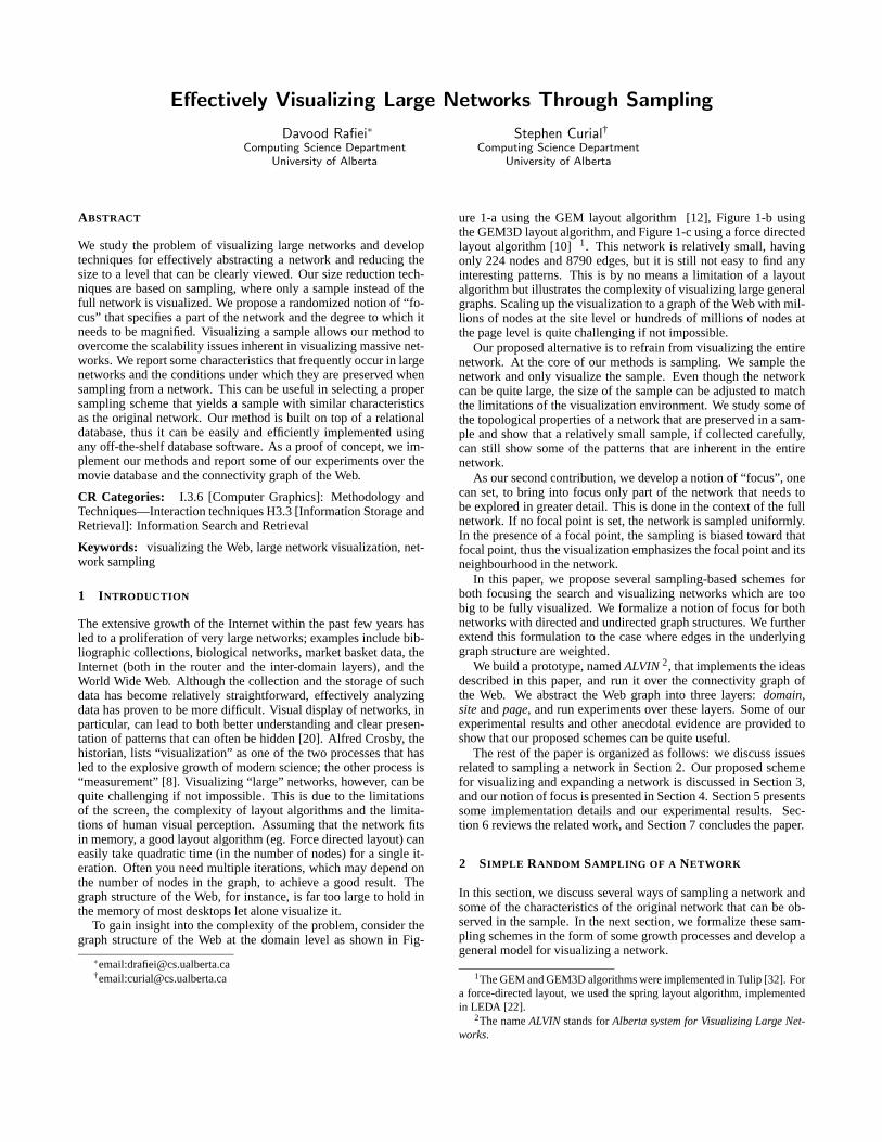
To gain insight into the complexity of the problem, consider thegraph structure of the Web at the domain level as shown in Fig-

∗email:[email protected]†email:[email protected]

ure 1-a using the GEM layout algorithm [12], Figure 1-b usingthe GEM3D layout algorithm, and Figure 1-c using a force directedlayout algorithm [10] 1. This network is relatively small, havingonly 224 nodes and 8790 edges, but it is still not easy to find anyinteresting patterns. This is by no means a limitation of a layoutalgorithm but illustrates the complexity of visualizing large generalgraphs. Scaling up the visualization to a graph of the Web with mil-lions of nodes at the site level or hundreds of millions of nodes atthe page level is quite challenging if not impossible.

Our proposed alternative is to refrain from visualizing the entirenetwork. At the core of our methods is sampling. We sample thenetwork and only visualize the sample. Even though the networkcan be quite large, the size of the sample can be adjusted to matchthe limitations of the visualization environment. We study some ofthe topological properties of a network that are preserved in a sam-ple and show that a relatively small sample, if collected carefully,can still show some of the patterns that are inherent in the entirenetwork.

As our second contribution, we develop a notion of “focus”, onecan set, to bring into focus only part of the network that needs tobe explored in greater detail. This is done in the context of the fullnetwork. If no focal point is set, the network is sampled uniformly.In the presence of a focal point, the sampling is biased toward thatfocal point, thus the visualization emphasizes the focal point and itsneighbourhood in the network.

In this paper, we propose several sampling-based schemes forboth focusing the search and visualizing networks which are toobig to be fully visualized. We formalize a notion of focus for bothnetworks with directed and undirected graph structures. We furtherextend this formulation to the case where edges in the underlyinggraph structure are weighted.

We build a prototype, named ALVIN 2, that implements the ideasdescribed in this paper, and run it over the connectivity graph ofthe Web. We abstract the Web graph into three layers: domain,site and page, and run experiments over these layers. Some of ourexperimental results and other anecdotal evidence are provided toshow that our proposed schemes can be quite useful.

The rest of the paper is organized as follows: we discuss issuesrelated to sampling a network in Section 2. Our proposed schemefor visualizing and expanding a network is discussed in Section 3,and our notion of focus is presented in Section 4. Section 5 presentssome implementation details and our experimental results. Sec-tion 6 reviews the related work, and Section 7 concludes the paper.

2 SIMPLE RANDOM SAMPLING OF A NETWORK

In this section, we discuss several ways of sampling a network andsome of the characteristics of the original network that can be ob-served in the sample. In the next section, we formalize these sam-pling schemes in the form of some growth processes and develop ageneral model for visualizing a network.

1The GEM and GEM3D algorithms were implemented in Tulip [32]. Fora force-directed layout, we used the spring layout algorithm, implementedin LEDA [22].

2The name ALVIN stands for Alberta system for Visualizing Large Net-works.

(a) (b) (c)

Figure 1: The connectivity network of the World Wide Web at the domain level. (a) Frick’s GEM layout algorithm is used, (b) GEM3D is used as the layoutalgorithm, and (c) a spring layout algorithm is used.

Given a network G(VG,EG), any subgraph of G can be treated asa sample of the network. Clearly, there are different ways of takinga subgraph and as a result there are many different sampling strate-gies. We use the following three methods for obtaining a simplerandom sample of a network. Independent of the strategy used, welet S(VS,ES) denote a simple random sample of G.

SRS1: Take a simple random sample of the nodes, VS, and letS(VS,ES) be the subgraph of G induced by VS (i.e. the subset ofthe vertices, VS, and edges with both endpoints in this subset).

SRS2: Take a simple random sample of the edges, ES, and let VS ⊂VG be the set of nodes that are incident to at least one edge in ES.

SRS3: Take a simple random sample S′(V ′S,E

′S) using SRS2 and let

S(VS,ES) be the subgraph of G induced by the nodes in V ′S.

Given a network of N nodes, SRS1 randomly selects n nodes andincludes all the edges between the selected nodes. Thus a node ofdegree k is expected to have a degree of k n

N in the sample. Thecaveat is that this number is expected to be almost zero unless thesample includes a large fraction of the nodes, k is large or both.

SRS2 may be more desirable when the sample size is small or thenetwork is not well-connected. This sampling is unbiased towardedges but not toward nodes. Nodes with large in- or out-degreesare more likely to be in the sample, and paths of length greater thanone are likely to form between them. This is not as problematic asit may look since those nodes are likely to form the backbone of thenetwork and it is good to have them in the sample.

SRS3 bears similarities to both SRS1 and SRS2. As in SRS2,nodes with large degrees are more likely to be included in the sam-ple. However, like SRS1, there is a direct relationship between thedegree of a node in the sample and its actual degree.

Other strategies for sampling a network are also feasible (e.g.see [21]) and can be used with our framework.

2.1 Using Sampling to Visualize Network Topology

There are a number of traits which are found in every network,and can be useful in describing the general topology of a network.These include degree distribution, connected component size dis-tribution, average path length, clustering coefficient, etc. Some ofthese traits can be preserved when sampling from a network. Thedegree distribution of the Web graph, in particular, provides strati-fied counts of the degrees, differentiating hubs and authorities from

other pages [6]. This property in turn can be useful in a visualiza-tion, as evidenced by some of our examples. The component sizedistribution is another important visual feature of a network (e.g.see the results reported for the Web graph [9]), and we often want itto be preserved in a sample. We discuss these features in the contextof the movie database from IMDb 3, where each actor is representedby a vertex and there is an undirected edge between two actors ifthe actors are cast together in the same movie.

2.1.1 Path Length and Clustering Coefficient

A class of networks, known as small-world networks, are character-ized by a short average path length and high clustering coefficient4.It is not clear if the average path length and the clustering coeffi-cients can be predicted from a sample. Consider G1 as a completegraph and G2 as a complete bipartite graph. The clustering coef-ficients of G1 is 1 and G2 is 0. For a small sample of both graphstaken using SRS2, the clustering coefficient may not be well-definedif the selected edges or nodes are not connected. After increasingthe sample size, the clustering coefficient for G1 can be either un-defined, if the sample is not connected, or any number in the range[0,1]. In the latter case, the clustering coefficient is dependent onthe selected edges and does not monotonically change with the sam-ple size. Similarly, the clustering coefficient for a sample of G2 willbe either undefined or zero again depending on the edges that are se-lected but not the sample size. Finding a sampling strategy that canprovide an estimate of the clustering coefficient for a general graphis an open problem. The average path length, on the other hand,is only defined between nodes that are connected. Two nodes thathave a path between them in a parent graph may not be connectedin a sample. This makes it difficult to infer a correlation betweenthe average path length of a sample and that of its parent graph ingeneral, but there are more specific cases where a correlation exists(e.g. when SRS1 is used for sampling).

2.1.2 Degree Distribution

Figures 2, 3 and 4 show the degree distributions respectively usingSRS1, SRS2 and SRS3 for sampling from the movie database; thesample size is varied from 5% to 100%. For SRS1 and SRS3, there is

3IMDb - Internet Movie Database (www.imdb.com)4The clustering coefficient gives the average degree to which vertices

adjacent to a node are adjacent to each other. See Watts[33] for definitions.

1

10

100

1000

10000

1 10 100 1000

Num

ber

of n

odes

Degree

Entire Graph80% Sample using SRS_160% Sample using SRS_140% Sample using SRS_120% Sample using SRS_15% Sample using SRS_1

Figure 2: Degree distribution using SRS1 for sampling.

1

10

100

1000

10000

100000

1 10 100 1000

Num

ber

of n

odes

Degree



1

10

100

1000

10000

1 10 100 1000

Num

ber

of n

odes

Degree



a direct relationship between the actual degree of a node and its de-gree in a sample. This is shown by a relatively constant gap betweenthe actual and estimated distributions; the gap becomes smaller forlarger samples. For SRS2, our samples overestimate the real distri-bution for smaller degrees and underestimate the real distributionfor larger degrees. This is consistent among all samples. As a re-sult, the degree distribution of even a 5% sample for degrees 4, 5and 6 is very close if not the same as the actual distribution. Over-all, the gap between the actual and the estimated distributions usingSRS2 is smaller than that of SRS1, and the gap between the actualand estimated distributions using SRS3 is smaller than that of SRS2.Our estimates using SRS3 must be treated with care. The depictedsample sizes show the fraction of edges selected in the first step ofthe sample only. The size of the sample after adding all edges be-tween the selected nodes in the second step can be larger and canvary from one network to another. For instance, a 5% sample inone case includes over 50% of the edges. This explains why theestimated and the actual distributions are very close.

2.1.3 Component Size Distribution

0.01

0.1

1

10

100

1 10

% o

f co

mpo

nent

s

Component size


Figure 5: Connected component size distribution for SRS1

0.01

0.1

1

10

100

1 10

% o

f co

mpo

nent

s

Component size



Figures 5, 6 and7 show the component size distributions of themovie database, respectively using strategies SRS1, SRS2 and SRS3

0.01

0.1

1

10

100

1 10

% o

f co

mpo

nent

s

Component size

Entire Graph80% Sample using SRS_360% Sample using SRS_340% Sample using SRS_320% Sample using SRS_3

5% Sample using SRS_3


for sampling. The sample size in both graphs is varied from 5%to 100%. A small and a consistent gap between the distributionsof a sample and the entire graph indicate that the sample closelyresembles the original data.

There have been some attempts to find a relationship betweenthe distribution of component sizes in a sample and the numberof components in the entire network. For transitive graphs 5, inparticular, Frank has shown that if the network is sampled usingSRS1, the resulting network can be used to find an unbiased estimateof the number of connected components of the entire network [11].

Theorem 1. Let the parent graph be transitive, and supposeS(VS,ES), a simple random sample taken using SRS1. Let v = |VS|.If Kr(S) denotes the number of connected components of size r inthe sample, then an unbiased estimate of the number of connectedcomponents in the parent graph is given by

M

∑r=1

(1−Cr)Kr(S)

where

Cr = (−1)r(

N − v+ r−1r

)(vr

)−1

,

N is the number of nodes in the parent graph, M ≤ v is a constantand the parent graph has no connected component of size largerthan M.

Both the proof and the variance of this estimate is given byFrank [11]. In practice, we are often interested in visualizing graphswhich are not transitive, hence this theorem is not directly applica-ble. However, there are some indications that the estimates maystill be a useful approximation for other graphs. Abusing the theo-rem, we tried using SRS2 with Frank’s estimate on synthetic data.Our synthetic data included graphs consisting of both complete con-nected and complete bipartite components. The component sizeswere generated randomly and varied from 4 to 80. The resultsshowed that Frank’s estimate used with SRS2, sampling only 25%of the edges, could accurately estimate the number of componentswith an average error of less than 8%.

5A graph is transitive if there is an edge between every connected pairof vertices.

3 NETWORK GROWTH

If the network that is being visualized is too large, it may not be fea-sible to preserve some of the desired topological properties of thenetwork in a small sample. To address this problem and to providea navigation scheme, we develop several growth processes, collec-tively referred to as network growth, that allows one to interactivelyvisualize a network.

In an interactive fashion to some degree similar to Web browsers,a visualization may start with a small subset of the network whichmay include a set of hand-picked nodes and edges or the result of aquery. This is useful for narrowing down the visualization to someof the interesting elements when the network is too large to be fullyvisualized. The visualization may proceed towards the goal by iter-atively growing the initial set. A novelty of our method is that someuser-controllable parameters describe how and to what degree thenetwork must be expanded. The expanded network often has moredetail about the elements being studied yet is small enough to bevisualized and internalized. After a few layers of expansion, thenetwork may become too large; this may be an indication that thebrowsing should switch to another small subset.

Let G(VG,EG) be the network that needs to be visualized andC(VC,EC), a subgraph of G, be the network that is currently dis-played on canvas. We want to select nodes from VG −VC and edgesfrom EG −EC and add them to C, thus expanding the network oncanvas with respect to G. Next, we discuss several ways of expand-ing a a network, formalizing our earlier sampling schemes in theform of some growth processes.

a7

b4

a3

c1

c11

c2 c3 c4 c5b11

d1

d3

d2

d4

e2e3

b1

c10

a8 a9 a10 a11 a12 a13 a14 a15 a16

a6a5a4a2

a1 b2b3

b5

b6

b7

b8b9b10

c6 c8c7 c9

e1

Figure 8: A network instance.

3.1 Global Growth

Sometimes we want to gain some insight into the general connectiv-ity structure of the network without specifying a pivotal point; or wemight be interested in only part of the network but want to browsethis part in the context of the entire network. We may achieve thisby taking a simple random sample of the network and visualizethe sample. One such sample can provide the general connectivitystructure of the network and maybe some common patterns with-out emphasizing one specific part. Clearly, the larger the sample,the more accurate the estimates; though a detailed sample may notalways be clearly visualized.

Definition 1. Let C be a subgraph of a parent network G. A globalgrowth of C with respect to G adds to C a simple random sample ofG taken using one of the sampling strategies from Section 2.

Example 3.1. Figure 8 shows an instance of a network with 45nodes and 55 edges. A simple random sample obtained using SRS2,with only six edges picked from the random ordering shown in theappendix is displayed in Figure 9-a. This sample, consisting of11% of the edges, shows some of the components of the parentnetwork; it has the same number of connected components as the

b1

d1 d2

a1 c1

a5b7

b1

cba

a5 b10b9 c9

c3

a1

a7 b10b9

c1

c2 c4c3

c7 c8 c9a12 a14a13

Figure 9: (a) a global growth, (b) a local growth with initial edges (a1,a5),(b1,b10) and (c) a local growth with initial edge (c3,c9).

parent network even though the components are not necessarily thesame.

3.2 Local Growth

We often know some of the nodes and maybe some of the edges ofa network and wish to find more nodes and edges that are some-how related to our starting set, or we may want to find out howour starting set is perceived within the general structure of the en-tire network. This can be done through sampling from the networksurrounding C and adding the sample to the canvas. The sampleincludes some of the edges that glue C to the rest of the network G.

Definition 2. Let C be a subgraph of a parent network G, and letI(VI ,EI) be the subgraph of G such that EI is the set of edges withone endpoint in VC and the other endpoint in VG −VC and VI is theset of nodes incident to any edge in EI . A local growth of C withrespect to G adds to C a simple random sample of I taken using oneof the strategies from Section 2.

Our local growth generalizes a sampling method, often referredto as snowball sampling, which is typical of a link-tracing designwhere a simple random sample or stratified random sample of unitsis selected and all other units linked to the initial sample are in-cluded or observed [31]. Unlike a snowball sample, the initial setin a local growth is not necessarily picked randomly; instead, it canbe the result of a user query. Furthermore, a local growth does notnecessarily include all edges linked to the initial set since this canbe too large.

Example 3.2. Figure 9-b shows the result of a local growth af-ter hand-picking the edges (a1,a5) and (b1,b10) from the networkin Fig 8 and adding 6 more edges selected using SRS2 through alocal growth. For our edge selection, we again use the random or-dering in the appendix but only add edges with one endpoint in{a1,a5,b1,b10}. As another example, Figure 9-c shows the resultafter hand-picking (c3,c9), doing a local growth using SRS3 whichadds 6 more edges (these edges are coloured blue) and further ex-tending the graph to include edges with both endpoints alreadyselected (these edges are coloured black). Compared to a globalgrowth that shows more of the structure of the entire network withless resolution, a local growth depicts a specific part of the networkin greater detail but with less information about the network as awhole.

3.3 Mixed Growth

A local growth can be combined with a global growth at a user-specified rate to provide a more balanced mixture of the two. Un-der this scheme, called a mixed growth, the network is sampled asfollows: with some probability we perform a local growth and withthe remaining probability we perform a global growth. A mixedgrowth provides a spectrum of sampling schemes with local andglobal growths at the two ends of the spectrum.

3.4 Wiring and Rewiring

Sometimes we have our desired nodes on canvas and wish to visual-ize the interconnections between them in greater detail. A solutionis to add more edges between the nodes on canvas. This is a spe-cial case of SRS2 where the sample is taken from the graph inducedby the nodes on canvas; we call this process wiring. In the ex-treme case, a wiring can add all the edges between nodes on canvas.However, this may clutter the visualization, hence a user-specifiedparameter may be used control the degree of wiring.

Since selecting edges is a random event, there are many possiblewirings, and we may wish to view more than one possible wiring ofthe nodes on canvas. Through the process of rewiring, all edges oncanvas can be removed and the nodes on canvas can be wired again.This may reveal properties that may not have been displayed by theoriginal wiring.

4 FOCUSED BROWSING

A network growth already provides a way to focus on a specificpart of the network, but the part of the network we can focus onis always fixed to I in a local growth and to G in a global growth.In general, we may want to focus on a part of the network otherthan I and G. We introduce a more general notion of focus that canbe used to narrow the visualization to a desired part of the network,reducing both the size and the complexity of the visualized network.Our notion of “focus”, referred to here as focal point, formulates tosome extent our interest in the network. Without loss of generality,our browsing goal is to visualize the focal point in the context ofthe entire network.

The following scenario shows how a focused browsing can beuseful. Consider the connectivity graph of the Web where nodesrepresent Web pages and edges describe the hyperlinks betweenpages. Suppose we are interested in the connectivity of pages on aspecific topic, say surfing. We can set the focal point to include allpages that mention the term ‘surfing’ in their contents. There canbe many more pages on this topic than what we can fit on canvas,thus we may visualize only a subset of these pages. If we expand thevisualized set by adding pages that either link to a page in the initialset or are linked by a page in the initial set, the resulting set is shownto include the most prominent sources of primary content knownas authorities and high-quality guides and resource lists known ashubs on the search topic[19].

It is not hard to integrate this notion of “focus” into our visual-ization scheme. Since our visualization is based on sampling, in thepresence of a focal point, the sampling is biased toward this focalpoint.

4.1 Formal Model

Given a network G(V,E), a focal point is a subgraph F(Vf ,E f )where Vf ⊆ V and E f ⊆ E. In the absence of a focal point, F isnaturally G, meaning that we are interested in the entire network.

A focused growth describes how the network on canvas can beexpanded using a sample of the parent network and with respect toa focal point F . Next, we define a focused growth which takes tworeal number parameters that control the degree of bias towards thefocal point, and can be used with either SRS2 or SRS3. A similardefinition can be formalized for SRS1 which is not discussed here.

Definition 3. Let C denote the graph on canvas and F denote the fo-cal point; both are subgraphs of a parent network G. Denote with EIthe set of edges that have one endpoint in F and the other endpointnot in F . Let the input parameter r ∈ [0,1] denote the probabilitythat one endpoint of a selected edge should be sampled from thefocal point and the input parameter s ∈ [0,1] denote the probabilitythat the other endpoint should also be sampled from the focal point.

A focused growth at rate (r,s) of the network on canvas C with re-spect to the focal point F and the parent graph G adds to C simplerandom samples of EI , EG and EF with sample sizes respectivelyproportional to s(1− r)+ r(1− s), (1− r)(1− s) and rs (the nodesincident on sampled edges are obviously selected).

A focused growth combines two simple random samples with asnowball sample at a user-specified rate. If we set the focal pointto the network on canvas and r = 1 and s = 0, a focused growthsimulates the local growth of Section 3.2. A focused growth alsosimulates the global growth of Section 3.1 if we set the focal pointagain to the network on canvas and r = 0 and s = 0. Varying thevalues of the parameters r and s, we can obtain other variations ofa network growth.

4.2 Directed and Weighted Networks

It is not hard to extend our proposed schemes to both directed andweighted networks. For a directed network, we may fix in advancethe fractions at which a source and a destination must be selectedfrom VF . One simple setting, for instance, is to set the ratios to50/50 or some other constant. An alternative is to allow the ratiosto be set during browsing using additional parameters.

In a weighted network, often the weight of an edge describes thestrength of the relationship between the two endpoints. In a com-muting network, for instance, each edge may be weighted to indi-cate the frequency of travels made in a day. If the network consistsof more than one level of abstraction, each node or each edge in amore general layer may be weighted and the weight may aggregatemultiple nodes or edges from a more specific layer. For instance,the connectivity graphs of the Web on the domain and site levels canbe seen as aggregations of the Web graph on the page level. If theweight of a node or an edge is treated as an indication of its impor-tance, we want to bias the visualization towards highly-weightededges. This is again possible within our sampling framework byreplacing a simple random sample with a weighted sample.

5 EXPERIMENTS

ALVIN, our current prototype implementing these ideas, has thefollowing highlights:

• It uses the DB2 relational database as its back-end data stor-age and querying engine. It makes no assumption on the sizeof the network and the back-end relational database can effi-ciently handle very large data sets.

• It provides an interface for both focusing and expanding thenetwork on canvas. It allows the user to interactively expandthe graph on canvas using parameters r, s and the size of thesample. Requests that arise from user interactions are mappedto SQL statements and are directed to the back-end SQL en-gine for an efficient evaluation.

• It is developed in C++ using the LEDA class library [22] andmakes use of the layout and graph algorithms that are avail-able in this library.

• Network abstraction and hierarchical views are supported bycreating tables and views in the relational database.

We ran ALVIN over the linkage structure of a snapshot of theWeb from Internet Archive 6. Each vertex in the dataset denoted a

6The Internet Archive is a public nonprofit organization that offers accessto historical collections that exist in digital format, including the snapshotsof the Web (www.archive.org)

Web page and each directed edge denoted a hyperlink, and the net-work was stored as relational tables. We also constructed two hier-archical views of the data in the site and the domain levels. Thesegraphs were weighted with the weight of an edge representing thenumber of links from one site (domain) to another. For efficiencyreasons, these views were pre-computed and physically stored. OurWeb graph was a snapshot taken in 1999 and included 178 millionnodes and 800 million edges. Next, we report some of our resultswith this data set.

5.1 Bow-Tie Shapes

The Web has been shown to be made up of a few distinct compo-nents: (1) a core in which every node can be reached from everyother node, (2) an ‘IN’ that includes the nodes that link to the corebut are not linked back, (3) an ‘OUT’ that contains the nodes thatcan be reached from the core but do not link to the core, and (4)the remaining set of nodes which cannot reach or be reached fromthe core but are connected to ‘IN’, ‘OUT’, both or neither. Thesecomponents are best represented using a bow-tie shape [6].

One question is if we can enumerate some of the instances ofthese components, in particular those that are relevant to our search.For instance, given a set of nodes, we may want to find othernodes which can form a bow-tie shape with our initial set. Theresult can give more details on the nature of the nodes in eachcomponent and the connections within and between the compo-nents. In an attempt to enumerate some of the members of thesecomponents, we started with three nodes which were believed tobe in the core; these included dir.yahoo.com, yahoo.com andyahoo.ca. We did 10 local growths, each time adding 50 edges,followed by a focused growth, adding 100 edges with p = q = 1and the focal point set to the network on canvas. SRS2 wasused for sampling. The result as shown in Figure 10 includedmore nodes in the core such as sec.yahoo.com, anglefire.comand ncsa.uiuc.edu interconnected with nodes in OUT such ascfa-www.harvard.edu and newscientist.com and nodes in INsuch as internetcollege.net and chess-space.com.

Figure 10: Instances of the bow-tie shape in the Web graph

5.2 Natural Clusters

Related pages on the Web often form clusters, for instance,if they are on the same topic. To visualize these clusterswithin our scheme, we started with a few nodes as our seedset. The seed set in one experiment included two news sites(news.bbc.co.uk and www.foxnews.com), two CS department

home pages (www.cs.wisc.edu and www.cs.cornell.edu) andthe Science Magazine home page (www.sciencemag.org). Wedid a global growth, taking a 0.1% sample using SRS1 and adding168,000 nodes to our initial set. We expected that a dense connec-tion between related pages will yield a high probability that thesepages are part of the same connected component. For clarity, Fig-ure 11-a shows only the components that include the pages in ourseed set. Three clusters are formed around our seed set: one clusterincludes the two CS departments with other CS departments suchas www.lcs.mit.edu added through the sampling. Another clusterincludes the two news sites, and the third cluster includes the Sci-ence Magazine. Comparing the degrees of the nodes in our seed set,the Science Magazine has a larger degree than the two news siteswhich in turn have larger degrees than the two CS departments.This is consistent with their actual degrees in the parent network.

To add more details of the interconnections and within a globalgrowth, we took another 0.1% sample of the nodes using SRS1.This combined with our earlier sample gave a 0.2% sample of thenodes. As shown in Figure 11-b, the nodes in our initial seed setnow form a single connected component. It is easy to see that theaverage path between the news sites and the Science magazine pageis shorter than the average path between the CS department homepages and the Science magazine page. Compared to the Fox News,the British Broadcasting Co. (BBC) has a shorter path to the Sci-ence magazine, possibly due to its coverage of the science articles.

Our results in this section provide a few instances wherea visualization based on our sampling methods can lead to abetter understanding of the network. They are not compre-hensive; they rather show how a combination of our samplingschemes and growth processes can provide a tool for analyzingand mining large networks. More results can be found online atwww.cs.ualberta.ca/∼database/ALVIN. A demo of ALVIN isalso presented in the World Wide Web Conference [30].

6 RELATED WORK

It has been noted that layout, abstraction, focus and interactionform the basis of visualizing large networks [23]. Our work ad-dresses the issues of focus, interaction and partly abstraction forlarge graphs through the use of sampling; any general graph layoutalgorithm can be used with our scheme.

There has been past work on layout and encoding schemes thattrade off the generality for scalability and clarity and can scale-up to large trees or more specific graphs. In particular, Mun-zner [24] constructs spanning trees to represent the structure of aclass of graphs with more tree-like structures, referred to as quasi-hierarchical graphs. The resulting tree is drawn inside a ball withfisheye distortion used to provide a focus-context view. Abello et al.[1] propose a hierarchical partitioning of the nodes based on char-acteristics such as the geographical locations that the nodes mayrepresent. Using these partitions, different navigation and visual-ization schemes can be constructed [2]. Our work is different fromthese in that we don’t make any assumption on the structure of thenetwork or the characteristics of the nodes. It shouldn’t be hard tointegrate our work with these methods to allow the visualization toscale up to either larger or more general networks.

The work on general multiscale abstraction methods allows oneto visualize either the global structure or the smaller components ofa large network (e.g. [4, 18]). These methods usually do a cluster-ing of the network and provide a coarser visualization between theclusters and a finer visualization within each cluster but not both atthe same time. Gansner et al. [14] propose a notion of a hybridgraph which allows the region of interest to be viewed in a finerlevel and within the coarser graph. Other abstraction techniquesinclude, but are not limited to, the work of Noik [25], Plaisant etal. [29] and Herman et al. [17]. Our work is orthogonal and com-

pliments these abstraction methods. Our methods can be appliedto a coarser view of a network when the coarser view is still toolarge to be fully visualized. Our use of biased sampling for focus-ing makes our work different from standard fisheye focusing tech-niques [13]. Our sampling strategies can also be applied as a pre-or post-processing step, allowing the integration of our method withother abstraction and focusing techniques.

Related to sampling from a large database, a number of algo-rithms have been proposed for efficiently sampling from a sin-gle table and also from the results of set union, intersection andjoin [26, 7]. A survey of these techniques before 1994 is givenby Olken [27]. Sampling is now supported in major commercialdatabases and is also part of the recent SQL standard [15].

Related to our work is also the more general work on analyzingsocial networks (e.g. [33], [3]), mining graphs [28], URL sam-pling [16, 5] and analyzing the graph structure of the Web [6].

7 CONCLUSIONS

A new probabilistic approach for effectively searching and visualiz-ing large networks is proposed, where only a sample instead of theentire network is visualized. There is no concept of a unique visu-alization in this scheme; instead there are many possible visualiza-tions, each corresponding to some random sample of the network.The effectiveness of a sample and, as a result, a visualization that isbased on that sample depends on the presence of the desirable pat-terns of the parent network in the sample. We have provided someevidence to show that indeed such patterns are preserved in a sam-ple. Given the limitations of the screen and the size of a sample, ourproposed scheme allows the search to be localized, thus increasingthe ratio of sample size to the size of the desired network and re-moving possible biases due to the sample size.

Our work touches some of the problems related to visualizing asample of a network. There are a number of issues that are open tofurther research. First, sampling has been largely used to approx-imately answer aggregation queries on large data sets, but there isnot much work on finding sampling strategies that can preserve ei-ther the local or global properties of a network. Further studies onthe subject can lead to more effective visualization schemes. Sec-ond, our work treats visualization as an incremental process thatmay lead to the goal after a number of growths. After each growth,a layout algorithm must be invoked to properly place the networkon the canvas. A new layout may not be coherent with the old oneand the elements in both layouts can be placed in different loca-tions of the screen. Further research may look into algorithms thatcan preserve the locality of the nodes and still generate an effectivelayout after each growth.AcknowledgmentsThis work is supported by Natural Sciences and Engineering Re-search Council of Canada. We like to thank the anonymous review-ers for their comments.

REFERENCES

[1] J. Abello, I. Finocchi, and J. Korn. Graph sketches. In Proc. ofthe IEEE Symposium on Information Visualization, pages 67–70, SanDiego, October 2001.

[2] J. Abello, J. Korn, and M. Kreuseler. Navigating giga-graphs. In Proc.of the working conference on advanced visual interfaces (AVI), 2002.

[3] L. Adamic and E. Adar. Friends and neighbors on the web. SocialNetworks, 25(3):211–230, 2003.

[4] D. Auber, Y. Chiricota, F. Jourdan, and G. Melancon. Multiscale vi-sualization of small world networks. In Proc. of IEEE Symposium onInformation Visualization, pages 75–81, 2003.

[5] Z. Bar-Yossef, A. Berg, S. Chien, J. Fakcharoenphol, and D. Weitz.Approximating aggregate queries about Web pages via random walks.

(a) (b)

Figure 11: A global growth (a) with the sample size set to 0.1% and (b) with the sample size set to 0.2%. In both cases, the seed set colored in green.

In Proc. of the VLDB Conference, pages 535–544, Cairo, September2000. Morgan Kaufmann.

[6] A. Broder, R. Kumar, F. Maghoul, P. Raghavan, S. Rajagopalan,R. Stata, A. Tomkins, and J. Wiener. Graph structure in the Web. InProc. of the World Wide Web Conference, pages 309–320, Amsterdam,May 2000.

[7] S. Chaudhuri, R. Motwani, and V. Narasayya. On random samplingover joins. In Proc. of the SIGMOD Conference, pages 263–274. ACMPress, 1999.

[8] A. Crosby. The Measure of Reality: Quantification in Western Europe,1250-1600. Cambridge University Press, 1997. A summary is onlineat www.stolaf.edu/other/ql/crosby.html.

[9] S. Dill, R. Kumar, K. Mccurley, S. Rajagopalan, D. Sivakumar, andA. Tomkins. Self-similarity in the Web. In Proc. of the VLDB Confer-ence, pages 69–78, September 2001.

[10] P. Eades. A heuristic for graph drawing. Congressus Numerantium,42:149–160, 1984.

[11] O. Frank. Estimation of the number of connected components in agraph by using a sampled subgraph. Scandinavian Journal of Statis-tics, 5:177–188, 1978.

[12] A. Frick, A. Ludwig, and H. Mehldau. A Fast Adaptive Layout Algo-rithm for Undirected Graphs. In Proceedings of Graph Drawing ’94,Lecture Notes in Computer Science 894, pages 388–403. Springer-Verlag, 1994.

[13] G. Furnas. Generalized fisheye views. In Proc. of the Conference onHuman Factors in Computing Systems, pages 16–23. ACM, 1986.

[14] E. Gansner, Y. Koren, and S. North. Topological fisheye views forvisualizing large graphs. In Proc. of the IEEE Symposium on Informa-tion Visualization, 2004.

[15] P. Haas and C. Koenig. A bi-level bernoulli scheme for database sam-pling. In Proc. of the SIGMOD Conference, pages 275–286, Paris,2004. ACM Press.

[16] M. Henzinger, A. Heydon, M. Mitzenmacher, and M. Najork. Onnear-uniform url sampling. In Proc. of the World Wide Web Confer-ence, pages 295–308, Amsterdam, May 2000. Elsevier Science.

[17] I. Herman, M. Marshall, G. Melancon, D. Duke, M. Delest, and J.-P.Domenger. Skeletal images as visual cues in graph visualization. InProc. of the Data Visualization, pages 13–29, 1999.

[18] J. Huotari, K. Lyytinen, and M. Niemel. Improving graphical infor-mation system model use with elision and connecting lines. ACMTransactions on Computer-Human Interaction, 11(1):26–58, March2004.

[19] J. Kleinberg. Authoritative sources in a hyperlinked environment. InProc. of ACM-SIAM Symposium on Discrete Algorithms, pages 668–677, January 1998.

[20] A. Klovdahl. A note on images of networks. Social Networks, 3:197–214, 1981.

[21] V. Krishnamurthy, J. Sun, M. Faloutsos, and S. Tauro. Sampling In-ternet topologies: how small can we go? In Proc. of InternationalConference on Internet Computing, Las Vegas, 2003.

[22] LEDA. class library. www.algorithmic-solutions.com/enleda.htm.[23] A. Mendelzon. Visualizing the world wide web. In Proc. of the work-

ing conference on advanced visual interfaces (AVI), 1996.[24] T. Munzner. Interactive visualization of large graphs and networks.

PhD thesis, Stanford University, 2000.[25] E. Noik. Dynamic fisheye views: combining dynamic queries and

mapping with database views. PhD thesis, University of Toronto,1996.

[26] F. Olken. Random Sampling from Databases. PhD thesis, Universityof California at Berkeley, 1993.

[27] F. Olken and D. Rotem. Random sampling from databases - a survey.Statistics and Computing, 5(1):25–42, March 1995.

[28] C. Palmer, P. Gibbons, and C. Faloutsos. Data mining on large graphs.In Proc. ACM Intl. Conf. on SIGKDD, pages 81–90, 2002.

[29] C. Plaisant, J. Grosjean, and B. Bederson. Spacetree: supporting ex-ploration in large node link tree, design evolution and empirical eval-uation. In Proc. of the IEEE Symposium on Information Visualization,pages 57–66, Boston, October 2002.

[30] D. Rafiei and S. Curial. ALVIN: a system for visualizing large net-works. In Poster Proc. of the World Wide Web Conference, May 2005.

[31] S. Thompson. Sampling. Wiley, 2nd edition, 2002.[32] Tulip. www.tulip-software.org.[33] D. Watts. Small worlds: the dynamics of networks between order and

randomness. Princeton University Press, 1999.

A A RANDOM ORDERING OF THE EDGES IN THE RUNNINGEXAMPLE OF SECTION 4

Our examples in Section 3 use the following random ordering ofthe edges shown in Figure 8: (b1,b10), (a1,a5), (c1,c3), (b1,b9),(d1,d2), (d3,d4), (a7,b11), (c2,c6), (c11,c7), (c11,c6), (a1,a7),(a5,a13), (c3,c8), (b1,b7), (a5,a14), (c3,c7), (a5,a12), (a7,a16),(a2,a9), (c1,c4), (c2,c9), (c4,c9), (d4,d1), (a2,a10), (c2,c8), (b1,b4),(c1,c5), (a1,a4), (b1,b3), (a4,a11), (b1,b5), (c3,c6), (a1,a2), (d2,d3),(c1,c2), (b1,b6), (c2,c7), (c11,c9), (c5,c9), (a1,a3), (b1,b11),(a7,a15), (c11,c10), (a1,a6), (b1,b8), (c4,c6), (e2,e3), (e1,e2),(c4,c8), (b1,b2), (c11,c8), (c5,c10), (a2,a8), (c4,c7), (c3,c9).

eﬀectively visualizing large networks through samplingdrafiei/papers/vis05.pdf · eﬀectively...

Documents