1

EEE 432

Measurement and Instrumentation

Lecture 4

Errors during the measurement process II

Prof. Dr. Murat Aşkar İzmir University of Economics Dept. of Electrical and Electronics Engineering

2

Classification of Error

Errors arising during the measurement process can be divided into two

groups, known as systematic errors and

Systematic Errors

– Sources of systematic error

– Errors due to environmental inputs

– Wear in instrument components

– Connecting leads

– Reduction of systematic error

• Careful instrument design, Method of opposing inputs, High-gain feedback,

Calibration, Manual correction of output reading, Intelligent instruments

Random errors

2

3

Random errors Random errors in measurements are caused by unpredictable

variations in the measurement system.

They are usually observed as small perturbations of the

measurement either side of the correct value, i.e. positive errors

and negative errors occur in approximately equal numbers for a

series of measurements made of the same constant quantity.

Therefore, random errors can largely be eliminated by calculating

the average of a number of repeated measurements, provided that

the measured quantity remains constant during the process of

taking the repeated measurements.

4

Random errors Statistical analysis - 1

Assume the measurements

{x1, x2, x3, x4, x5, x6, x7, x8, x9}

Mean (Average)

Xmean = (x1+x2+x3+x4+x5+x6+x7+x8+x9) / 9

Median

The median is the middle value when the measurements in

the data set are written down in ascending order of

magnitude. For the above set fifth value is the median.

3

5

Random errors Statistical analysis - 2

Example 1

Measurement Set A (11 measurements)

398 420 394 416 404 408 400 420 396 413 430

Xmean = 409, Xmedian = 408,

Example 2

Measurement Set B (11 measurements)

409 406 402 407 405 404 407 404 407 407 408

Xmean = 406, Xmedian = 407,

Which one is more realiable?

6

Random errors Statistical analysis - 3

Example 3

Measurement Set C (23 measurements)

409 406 402 407 405 404 407 404 407 407 408 406 410

406 405 408 406 409 406 405 409 406 407

Xmean = 406.5, Xmedian = 406,

The median value tends towards the mean value as the

number of measurements increases

4

7

Random errors Statistical analysis - 4

Variance and Standard Deviation

– Deviation (error) in each measument

– Variance

– Standard Deviation

8

Random errors Statistical analysis - 5

Measurement Set A (11 measurements)

398 420 394 416 404 408 400 420 396 413 430

Xmean = 409, V = 137, = 11.7

Measurement Set B (11 measurements)

409 406 402 407 405 404 407 404 407 407 408

Xmean = 406, V = 4.2, = 2.05

Measurement Set C (23 measurements)

409 406 402 407 405 404 407 404 407 407 408 406 410

406 405 408 406 409 406 405 409 406 407

Xmean = 406.5, V = 3.53, = 1.88

5

9

Random errors Statistical analysis - 6

Note that the smaller values of V and for measurement set B

compared with A correspond with the respective size of the spread

in the range between maximum and minimum values for the two

sets.

Thus, as V and decrease for a measurement set, we are able to

express greater confidence that the calculated mean or median

value is close to the true value, i.e. that the averaging process has

reduced the random error value close to zero.

Comparing V and for measurement sets B and C, V and get

smaller as the number of measurements increases, confirming that

confidence in the mean value increases as the number of

measurements increases.

10

Graphical Data Analysis Histogram

Measurement Set C (23 measurements)

409 406 402 407 405 404 407 404 407 407 408 406 410

406 405 408 406 409 406 405 409 406 407

The simplest way of doing

this is to draw a histogram, in

which bands of equal width

across the range of

measurement values

are defined and the number

of measurements within each

band is counted.

6

11

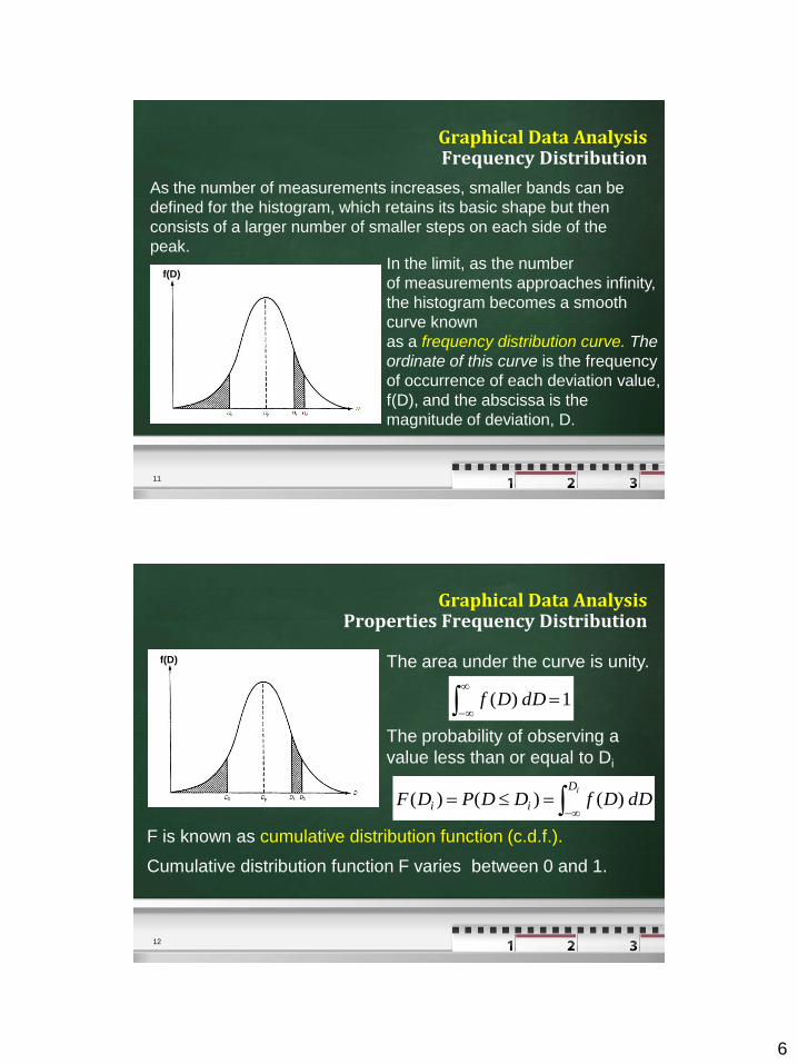
Graphical Data Analysis Frequency Distribution

As the number of measurements increases, smaller bands can be

defined for the histogram, which retains its basic shape but then

consists of a larger number of smaller steps on each side of the

peak.

In the limit, as the number

of measurements approaches infinity,

the histogram becomes a smooth

curve known

as a frequency distribution curve. The

ordinate of this curve is the frequency

of occurrence of each deviation value,

f(D), and the abscissa is the

magnitude of deviation, D.

f(D)

12

Graphical Data Analysis Properties Frequency Distribution

F is known as cumulative distribution function (c.d.f.).

Cumulative distribution function F varies between 0 and 1.

The area under the curve is unity.

The probability of observing a

value less than or equal to Di

f(D)

1)(

dDDf

dDDfDDPDFiD

ii )()()(

7

13

Graphical Data Analysis Gaussian distribution

For D = x - m, then f(D) is known as the error frequency

distribution.

The Gaussian distribution is

defined as.

where m is the mean and is the

standart deviation m x

f(x)

222/

2πσ

1)( mxexf

22 2/

2πσ

1)( DeDf

14

Graphical Data Analysis Standard Gaussian distribution

The new form called standard Gaussian curve.

and

Substituting

a new Gaussian distribution with

zero mean (m=0) and unit

standard deviation (=1), is

obtained.

f(z)

2/2

2π

1)( zezf dzezF

zz

2/2

2π

1)(

8

15

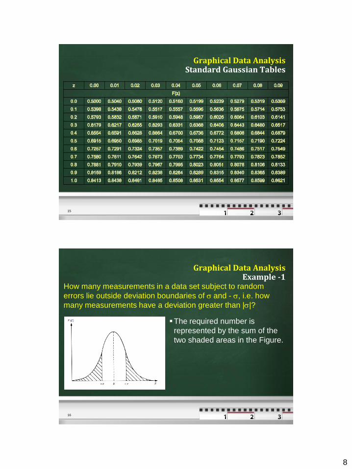
Graphical Data Analysis Standard Gaussian Tables

16

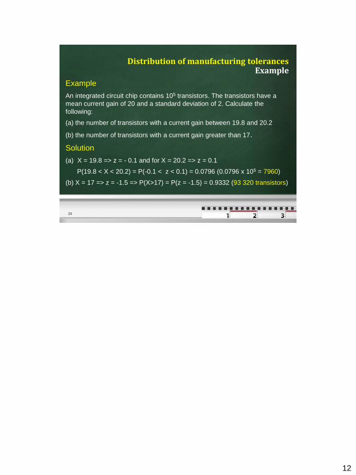
Graphical Data Analysis Example -1

How many measurements in a data set subject to random

errors lie outside deviation boundaries of and - , i.e. how

many measurements have a deviation greater than ||?

The required number is

represented by the sum of the

two shaded areas in the Figure.

9

17

Graphical Data Analysis Example - 2

P(E < - or E > +) = P(E < -) + P(E > +)

If E = -, then z = -1 and hence

P(E < -) = F(z = -1) = 1 – F(1) = 1 – 0.8413 = 0.1587

F(1) = 0.8413 (from Gaussian Table)

Similarly, P(E > ) = 1 – F(1) = 1 - 0.8413 = 0.1587.

Then P(E < -) + P(E > +) = 0.1587+0.1587=0.3174 = 31.74 %

i.e. 32% of the measurements lie outside the ± boundaries,

then 68% of the measurements lie inside.

18

Graphical Data Analysis Example - 3

Deviation boundaries % of data points within

boundary

Probability of any

particular data point

being outside boundary

± 68.0 32.0 %

±2 95.4 4.6 %

±1.96 95.0 0.3%

±2 95.0 0.3%

±3 99.7 0.3%

10

19

Graphical Data Analysis Standard error of the mean

The error between the mean of a finite data set and the true

measurement value (mean of the infinite data set) is defined as

the standard error of the mean, . This is calculated as

The measurement value obtained from a set of n measurements,

{x1, x2, ........., xn}

20

Standard error of the mean Example

Measurement Set C (23 measurements)

409 406 402 407 405 404 407 404 407 407 408 406 410 406

405 408 406 409 406 405 409 406 407

Xmean = 406.5, V = 3.53, = 1.88 and = 0.39

The length can therefore be expressed as 406.5 ± 0.4 (68%

confidence limit).

However, it is more usual to express measurements with 95%

confidence limits (± 2 boundaries).

– In this case, 2 = 3.76, = 0.78 and the length can be expressed

as 406.5 ± 0.8 (95% confidence limits).

11

21

Standard error of the mean Estimation of random error in a single measurement

For 95% confidence interval, the maximum likely deviation in a

single measurement is ±1.96. However, this only expresses

the maximum likely deviation of the measurement from the

calculated mean of the reference measurement set, which is

not the true value as observed earlier. Thus the calculated

value for the standard error of the mean has to be added to

the likely maximum deviation value. Thus, the maximum likely

error in a single measurement can be expressed as:

Error = ± (1.96 +

22

Estimation of random error in a single measurement Example

Example

Suppose that a standard mass is measured 30 times with the same

instrument to create a reference data set, and the calculated values of

and are 0.43 and = 0.08. If the instrument is then used to

measure an unknown mass and the reading is 105.6 kg, how should

the mass value be expressed under %95 confidence interval?

Solution

Error = ± (1.96 + ) = 0.92

The mass value should therefore be expressed as:

105.6 ± 0.9 kg.

12

23

Distribution of manufacturing tolerances Example

Example

An integrated circuit chip contains 105 transistors. The transistors have a

mean current gain of 20 and a standard deviation of 2. Calculate the

following:

(a) the number of transistors with a current gain between 19.8 and 20.2

(b) the number of transistors with a current gain greater than 17.

Solution

(a) X = 19.8 => z = - 0.1 and for X = 20.2 => z = 0.1

P(19.8 < X < 20.2) = P(-0.1 < z < 0.1) = 0.0796 (0.0796 x 105 = 7960)

(b) X = 17 => z = -1.5 => P(X>17) = P(z = -1.5) = 0.9332 (93 320 transistors)