eee436closed loop controllers - İtÜweb.itu.edu.tr/yalcinme/files/courses/mmg/ch13 closed...

1

Bolton, Mechatronics PowerPoints, 4th Edition, © Pearson Education Limited 2008

Figure 15.1 Unity feedback

Feedback Control system

2


Advantages of Feedback in Control Compared to open-loop control, feedback can

be used to:

• Reduce the sensitivity of a system’s transfer function to parameter changes

• Reduce steady-state error in response to disturbances,

• Reduce steady-state error in tracking areference response (& speed up the transient response)

• Stabilize an unstable process

3


Disadvantages of Feedback in Control

Compared to open-loop control,

• Feedback requires a sensor that can be very expensive and may introduce additional noise

• Feedback systems are often more difficult to design and operate than open-loop systems

• Feedback changes the dynamic response (faster) but often makes the system less stable.

4


Unit step response of a 2nd order under-damped system

,eM,.

t,t,.

t /pspr

21

000

6481 ζπζ

ζωωπ

ω−−=≅≅≅

5


Transient Response vs Simple Pole Locations

)(sRe

)(sIm

)(ty )(ty

)(ty

t

t

t

)(ty

t

)(ty

t

)(ty

t

6


Figure 15.15 Control system

Controlled system

7


Control Modes• There are a number of ways by which a control unit can

be react to an error signal and supply an output for correcting elements:

• 1- two step mode: the controller is an ON-OFF correcting signal

• 2- The proportional Mode: the controller produce a control action proportional to the error.

• 3: the derivative mode D: the controller produces a control action proportional to the rate at which the error is changing. When there is a sudden change in the error signal, the controller gives alarge correcting signal, when there is a gradual change only a small correcting signal is produces. Normally used in conjunction with proportional control

8


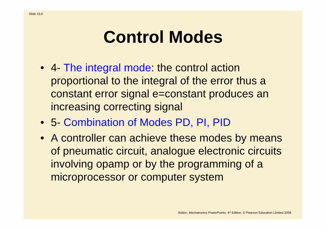
• 4- The integral mode: the control action proportional to the integral of the error thus a constant error signal e=constant produces an increasing correcting signal

• 5- Combination of Modes PD, PI, PID• A controller can achieve these modes by means

of pneumatic circuit, analogue electronic circuits involving opamp or by the programming of a microprocessor or computer system

Control Modes

9

Bolton, Mechatronics PowerPoints, 4th Edition, © Pearson Education Limited 2008Figure 15.2 Two-step control

Two step modeAn example of two step mode of control id the bimetallic thermostat that might be used with a simple temperature control system.

10


• Consequences:• To avoid continuous

switching ON and OFF on respond to slight change, two values are normally used, a dead band is used for the values between the ON and OFF values

• Large dead band implieslarge temp. fluctuations

• Small dead band increaseswitching frequency

Two step mode

11


Two step mode•The bimetallic element has permanent magnet for a switch contact, this has the effect of producing a dead band.Fast ON-OFF control can be used for motor control using controlled switching elements (IGBT, BJT, MOSFET, Thyrester)

12


Proportional Mode• With the two step method of control, the

controller output is either ON or OFF signal, regardless of the magnitude of error.

• With proportional control mode, the size of the controller output is proportional to the size of the error. The bigger the error the bigger the output from the controller

• Controller output u(t) = Kp e

• Or in s domain U(s)=KpE(s)

13

Bolton, Mechatronics PowerPoints, 4th Edition, © Pearson Education Limited 2008Figure 15.3 Proportional controller

Electronic Proportional ModeA summing opamp with an inverter can be used as proportional controller

The output from the summing amplifier is

14


Electronic Proportional Mode

15

Bolton, Mechatronics PowerPoints, 4th Edition, © Pearson Education Limited 2008Figure 15.4 Proportional controller for temperature control

Electronic Proportional Mode

16


System response to proportional control

17


Derivative control mode

As soon as the error signal begins to change, there can be quite a large controller output, thus rapid initial response to error signal occur

In Figure the controller output is constant is constant because the rate of change is constant.

18


• - They do not response to steady- state error signal, that is why always combined with P-controller

• P responds to all error• D responds to rate of change• Derivative action can also be a problem if the

measurement of the process variable gives a noisy signal, the rapid fluctuations of the noise resulting in outputs which will be seen by the controller as rapid changes in error and so give rise to significant outputs from the controller.


19


Figure 15.7 Derivative controller


The Figure shows the form of an electronic derivative controller circuit, it composed of two operational amplifier: integrator + Inverter

20


PD controller

21


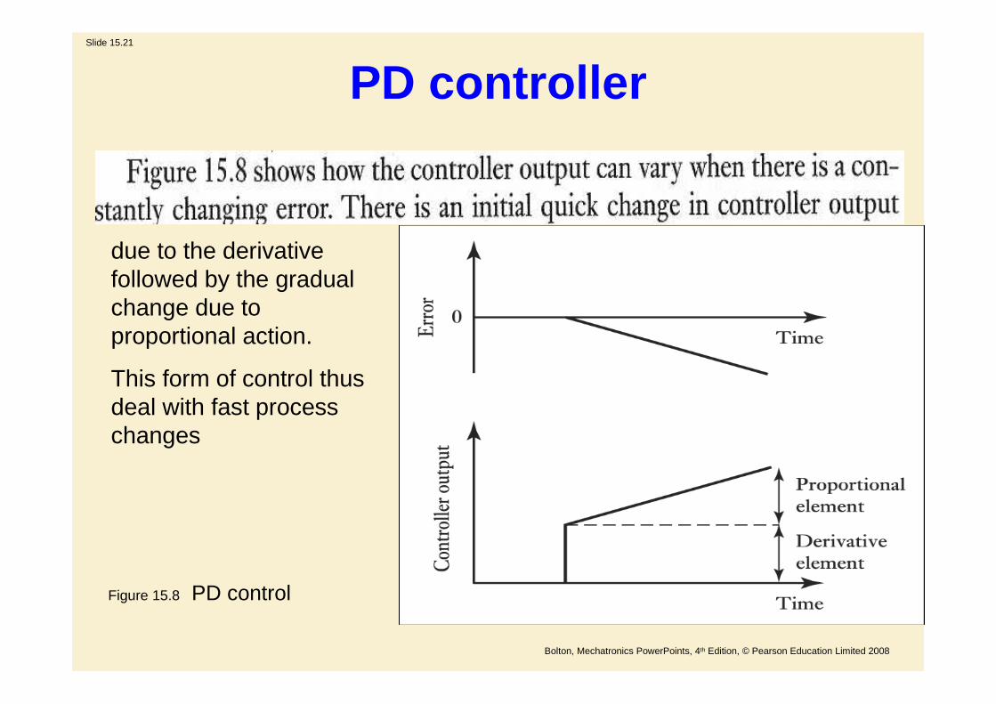
Figure 15.8 PD control

PD controller

due to the derivative followed by the gradual change due to proportional action.

This form of control thus deal with fast process changes

22


Integral control

23


Figure 15.9 Integral control

Integral control

Figure shows the action of an integral controller when there is a constant error input to the controller

When the controller output is constant, the error is zero; when controller output is varies at a constant rate, the error has a constant value.

24


Figure 15.10 Electronic Integral controller

Integral controlThe integrator is connected to the error signal at time t, whilethe second integrator is connected to the error at t=0- i.e. (t-Ts)

25


PI control

26


Figure 15.11 PI control

PI control

27


PID Controller

28


PID circuit

29


PID & Closed-loop Response

Small change

DecreaseDecreaseSmall change

D

EliminateIncreaseIncreaseDecreaseI

DecreaseSmall change

IncreaseDecreaseP

Steady-state error

Settling time

Maximum overshoot

Rise time

• Note that these correlations may not be exactly accurate, because P, I and D gains are dependent of each other.

30


PID Response

PDP

PI PID

31


PID Conclusions• Increasing the proportional feedback gain

reduces steady-state errors, but high gains almost always destabilize the system.

• Integral control provides robust reduction in steady-state errors, but often makes the system less stable.

• Derivative control usually increases damping and improves stability, but has almost no effect on the steady state error

• These 3 kinds of control combined from the classical PID controller

32


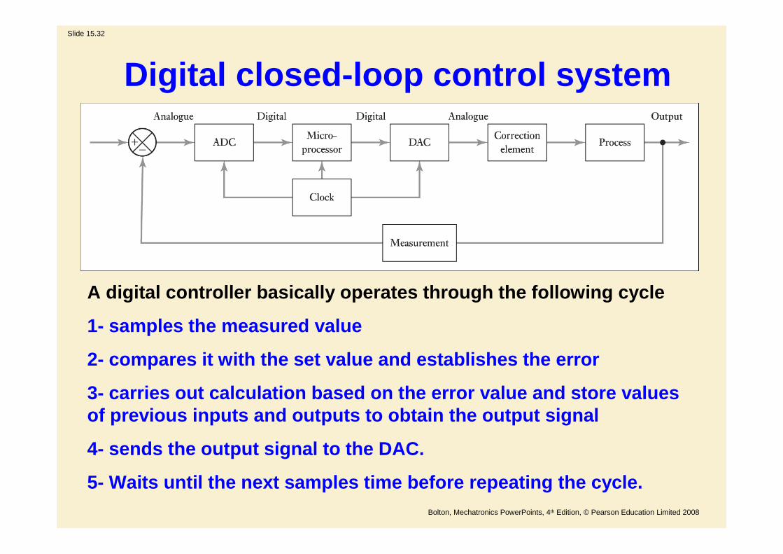
Digital closed-loop control system

A digital controller basically operates through the following cycle

1- samples the measured value

2- compares it with the set value and establishes the error

3- carries out calculation based on the error value and store values of previous inputs and outputs to obtain the output signal

4- sends the output signal to the DAC.

5- Waits until the next samples time before repeating the cycle.

33


Digital PID Controller

34


Figure 15.18 System with velocity feedback: (a) descriptive diagram of the system,(b) block diagram of the system

35


Analog control of permanent magnet DC Motor

• Permanent magnet DC Motor are widely used in servo systems.• Figure: Schematic diagram of rotating table actuated by permanent

magnet motor

raa kE ω=

rgearky θ=rθ

mB

LT

trr ω=θer T,ω

36



• The angular displacement of the positioning table = the output equation

• To control the motor angular velocity wr, as well as angular displacement θr, and rotating table kgear θr, one regulates the armature voltage applied to the motor winding ua.

• To guarantee the stability, to attain the desired accuracy, to ensure tracking and disturbance attenuation of the servo system, one should design the control algorithm, and the coefficient of PID controller must be found.

• Find the transfer function. Obtained using differential equations that describe the system dynamics.

• Induced emf :

rgearkty θ=)(

raa kE ω= ak

rω

: Back emf constant

: angular velocity

37



• Using KVL:

• Applied Newtonian mechanics to find the differential equations for mechanical systems.

• Using Newton’s second law:

• Electromagnetic torque developed by permanent magnet DC motor:

• Viscous torque :

• Load torque : TL

aa

ra

aa

a

a uLL

ki

L

r

dt

di 1+ω−−=

dt

dJJT

ω=α=∑r

rr

J : equivalent moment of inertia

aae ikT =ak : Torque constant = Back emf constant

rmviscous BT ω=

38



• Using Newton’s second law :

• Dynamics of rotor angular displacement :

• The derived three first order differential equations are rewritten in the s-domain

( ) ( )LrmaaLviscouser TBik

JTTT

Jdt

d −ω−=−−=ω 11

rr

dt

d ωθ

)(1

)()( suL

sL

ksi

L

rs a

ar

a

aa

a

a +ω−=

+

)(1

)(1

)( sTJ

sikJ

sJ

Bs Laar

m −=ω

+

)()( sss rr ω=θ

39



• Block diagram of closed loop the permanent magnet DC motor :

40



• The controller should be designed, and the output equation:• Using this output equation, as well as • Block diagram of open loop servo actuated by permanent magnet DC

motor :

rgearkty θ=)(

)(ss rr ω=θ

41



• Using the linear PID controller:

• Block diagram of closed loop servo actuated by permanent magnet DC motor with the linear PID controller :

)()()()( tsektes

ktektu d

ipa ++=

42


TUNING THE PID CONTROLLER

Ziegler-Nichols Tuning Rules

• 1. SET KP. Starting with KP=0, KI=0 and KD=0, increase KP until the output starts overshooting and ringing significantly.

• 2. SET KD. Increase KD until the overshoot is reduced to an acceptable level.

• 3. SET KI. Increase KI until the final error is equal to zero.

43



44



45


Figure 15.20 Self-tuning

46


Figure 15.21 Model-referenced control

eee436closed loop controllers - İtÜweb.itu.edu.tr/yalcinme/files/courses/mmg/ch13 closed...

Documents