eelleeccttrroommaaggnneettiicc tthheeoorryythegateacademy.com/files/wppdf/electromagnetics.pdf ·...
TRANSCRIPT
EElleeccttrroommaaggnneettiicc TThheeoorryy
FFoorr
EElleeccttrriiccaall EEnnggiinneeeerriinngg
By
www.thegateacademy.com
Syllabus
: 080-617 66 222, [email protected] ©Copyright reserved. Web:www.thegateacademy.com
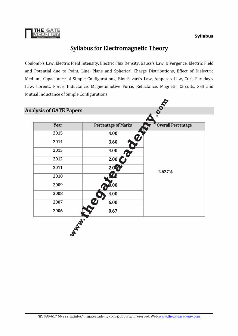
Syllabus for Electromagnetic Theory
Coulomb's Law, Electric Field Intensity, Electric Flux Density, Gauss's Law, Divergence, Electric Field
and Potential due to Point, Line, Plane and Spherical Charge Distributions, Effect of Dielectric
Medium, Capacitance of Simple Configurations, Biot‐Savart’s Law, Ampere’s Law, Curl, Faraday’s
Law, Lorentz Force, Inductance, Magnetomotive Force, Reluctance, Magnetic Circuits, Self and
Mutual Inductance of Simple Configurations.
Analysis of GATE Papers
Year Percentage of Marks Overall Percentage
2015 4.00
2.627%
2014 3.60
2013 4.00
2012 2.00
2011 2.00
2010 0.00
2009 0.00
2008 4.00
2007 6.00
2006 0.67
Contents
: 080-617 66 222, [email protected] ©Copyright reserved. Web:www.thegateacademy.com i
CCoonntteennttss
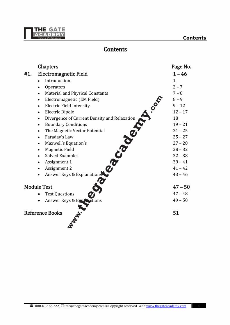
Chapters Page No.
#1. Electromagnetic Field 1 – 46 Introduction 1
Operators 2 – 7
Material and Physical Constants 7 – 8
Electromagnetic (EM Field) 8 – 9
Electric Field Intensity 9 – 12
Electric Dipole 12 – 17
Divergence of Current Density and Relaxation 18
Boundary Conditions 19 – 21
The Magnetic Vector Potential 21 – 25
Faraday’s Law 25 – 27
Maxwell’s Equation’s 27 – 28
Magnetic Field 28 – 32
Solved Examples 32 – 38
Assignment 1 39 – 41
Assignment 2 41 – 42
Answer Keys & Explanations 43 – 46
Module Test 47 – 50
Test Questions 47 – 48
Answer Keys & Explanations 49 – 50
Reference Books 51
:080-617 66 222, [email protected] ©Copyright reserved. Web:www.thegateacademy.com 1
“Picture yourself vividly as winning and that
alone will contribute immeasurably to success."
…Harry Fosdick
Electromagnetic
Field
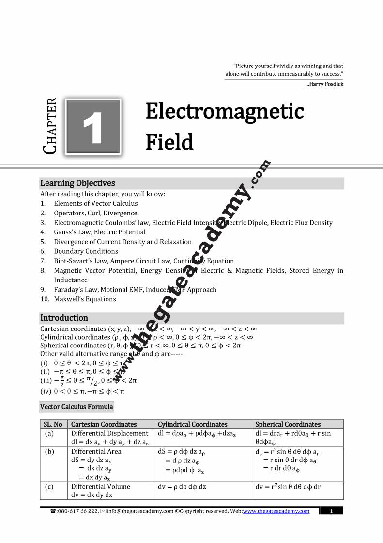
Learning Objectives After reading this chapter, you will know:
1. Elements of Vector Calculus
2. Operators, Curl, Divergence
3. Electromagnetic Coulombs’ law, Electric Field Intensity, Electric Dipole, Electric Flux Density
4. Gauss's Law, Electric Potential
5. Divergence of Current Density and Relaxation
6. Boundary Conditions
7. Biot-Savart’s Law, Ampere Circuit Law, Continuity Equation
8. Magnetic Vector Potential, Energy Density of Electric & Magnetic Fields, Stored Energy in
Inductance
9. Faraday’s Law, Motional EMF, Induced EMF Approach
10. Maxwell’s Equations
Introduction Cartesian coordinates (x, y, z), −∞ < x < ∞, −∞ < y < ∞, −∞ < z < ∞ Cylindrical coordinates (ρ , ϕ, z), 0 ≤ ρ < ∞, 0 ≤ ϕ < 2π, −∞ < z < ∞ Spherical coordinates (r, θ, ϕ ) , 0 ≤ r < ∞, 0 ≤ θ ≤ π, 0 ≤ ϕ < 2π Other valid alternative range of θ and ϕ are-----
(i) 0 ≤ θ < 2π, 0 ≤ ϕ ≤ π (ii) −π ≤ θ ≤ π, 0 ≤ ϕ ≤ π
(iii) −π
2≤ θ ≤ π
2⁄ , 0 ≤ ϕ < 2π
(iv) 0 < θ ≤ π,−π ≤ ϕ < π
Vector Calculus Formula
SL. No Cartesian Coordinates Cylindrical Coordinates Spherical Coordinates
(a) Differential Displacement dl = dx ax + dy ay + dz az
dl = dρaρ + ρdϕaϕ +dzaz dl = drar + rdθaθ + r sin θdϕaϕ
(b) Differential Area dS = dy dz ax = dx dz ay
= dx dy az
dS = ρ dϕ dz aρ
= d ρ dz aϕ
= ρdρd ϕ az
ds = r2sin θ dθ dϕ ar = r sin θ dr dϕ aθ = r dr dθ aϕ
(c) Differential Volume dv = dx dy dz
dv = ρ dρ dϕ dz dv = r2sin θ dθ dϕ dr
CH
AP
TE
R
1
Electromagnetic Field
: 080-617 66 222, [email protected] ©Copyright reserved. Web:www.thegateacademy.com 2
Operators 1) ∇ V – Gradient, of a Scalar V
2) ∇ V – Divergence, of a Vector V
3) ∇ × V – Curl, of a Vector V
4) ∇2 V – Laplacian, of a Scalar V
DEL Operator:
∇ =∂
∂xax +
∂
∂yay +
∂
∂z az(Cartesian)
= ∂
∂ρaρ +
1
ρ
∂
∂ϕaϕ +
∂
∂z az(Cylindrical)
=∂
∂rar +
1
r
∂
∂θaθ +
1
rsi n θ ∂
∂ϕ aϕ(Spherical)
Gradient of a Scalar field
V is a vector that represents both the magnitude and the direction of maximum space rate of
increase of V.
∇V =∂V
∂xax +
∂V
∂yay +
∂V
∂z az For Cartisian Coordinates
=∂V
∂ρaρ +
1
ρ
∂V
∂ϕaϕ +
∂V
∂z az For Spherical Coordinates
=∂V
∂rar +
1
r
∂V
∂θaθ +
1
rsi n θ ∂V
∂ϕ aϕ For Cylindrical Coordinates
The following are the fundamental properties of the gradient of a scalar field V
1. The magnitude of ∇V equals the maximum rate of change in V per unit distance.
2. ∇V points in the direction of the maximum rate of change in V.
3. ∇V at any point is perpendicular to the constant V surface that passes through that point.
4. If A = ∇V, V is said to be the scalar potential of A.
5. The projection of ∇V in the direction of a unit vector a is ∇V. a and is called the directional
derivative of V along a. This is the rate of change of V in direction of a.
Example: Find the Gradient of the following scalar fields:
(a) V = e−z sin 2x cosh y
(b) U = ρ2z cos 2ϕ
(c) W = 10r sin2θ cos ϕ
Solution:
(a) ∇V =∂V
∂xax +
∂V
∂yay +
∂V
∂zaz
= 2e−z cos 2x cosh y ax + e−z sin 2x sinh y ay − e−z sin 2x cosh y az
(b) ∇U =∂U
∂ρaρ +
1
ρ
∂U
∂ϕaϕ +
∂U
∂zaz
= 2ρz cos 2ϕ aρ − 2ρz sin 2ϕ aϕ + ρ2 cos 2 ϕ az
(c) ∇W =∂W
∂rar +
1
r
∂W
∂θaθ +
1
r sinθ
∂W
∂ϕaϕ
= 10 sin2θ cos ϕ ar + 10 sin 2θ cos ϕ aθ − 10 sin θ sinϕ aϕ
Electromagnetic Field
: 080-617 66 222, [email protected] ©Copyright reserved. Web:www.thegateacademy.com 3
Divergence of a Vector
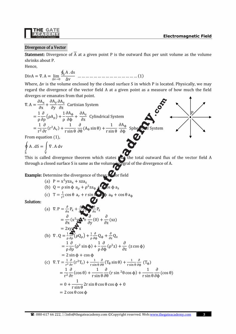
Statement: Divergence of A at a given point P is the outward flux per unit volume as the volume
shrinks about P.
Hence,
DivA = ∇. A = lim∆v→0
∮ A . ds
S
∆v ………… ………………………… …(1)
Where, ∆v is the volume enclosed by the closed surface S in which P is located. Physically, we may
regard the divergence of the vector field A at a given point as a measure of how much the field
diverges or emanates from that point.
∇. A =∂Ax
∂x+
∂Ay
∂y
∂Az
∂z Cartisian System
=1
ρ
∂
∂ρ(ρAρ) +
1
ρ
∂Aϕ
∂ϕ+
∂Az
∂z Cylindrical System
=1
r2
∂
∂r(r2Ar) +
1
r sin θ ∂
∂θ(Aθ sinθ) +
1
r sin θ ∂Aϕ
∂ϕ Sphearical System
From equation (1),
∮A . dS
S
= ∫∇ . A dv
V
This is called divergence theorem which states that the total outward flux of the vector field A
through a closed surface S is same as the volume integral of the divergence of A.
Example: Determine the divergence of these vector field
(a) P = x2yzax + xzaz
(b) Q = ρ sinϕ aρ + ρ2zaϕ + z cos ϕ az
(c) T =1
r2 cos θ ar + r sin θ cos ϕ aθ + cosθ aϕ
Solution:
(a) ∇. P =∂
∂xPx +
∂
∂yPy +
∂
∂zPz
=∂
∂x(x2yz) +
∂
∂y(0) +
∂
∂z(xz)
= 2xyz + x
(b) ∇ . Q =1
ρ
∂
∂ρ(ρQρ) +
1
ρ
∂
∂ϕQϕ +
∂
∂zQz
=1
ρ
∂
∂ρ(ρ2 sinϕ) +
1
ρ
∂
∂ϕ(ρ2z) +
∂
∂z (z cos ϕ)
= 2 sinϕ + cos ϕ
(c) ∇. T =1
r2
∂
∂r(r2Tr) +
1
r sinθ
∂
∂θ(Tθ sinθ) +
1
r sin θ
∂
∂ϕ (Tϕ)
=1
r2
∂
∂r(cos θ) +
1
r sin θ
∂
∂θ(r sin 2θ cos ϕ) +
1
r sin θ
∂
∂ϕ(cos θ)
= 0 +1
r sinθ2r sin θ cos θ cos ϕ + 0
= 2cos θ cosϕ
P
Electromagnetic Field
: 080-617 66 222, [email protected] ©Copyright reserved. Web:www.thegateacademy.com 4
Curl of a Vector
Curl of a Vector field provides the maximum value of the circulation of the field per unit area and
indicates the direction along which this maximum value occurs.
That is,
Curl A = ∇ × A = limΔS→0
(∮ A . dl
L
∆S)
max
an ……… ………… . . (2)
∇ × A = ||
ax ay az
∂
∂x
∂
∂y
∂
∂zAx Ay Az
||
= 1
ρ ||
aρ ρaϕ az
∂
∂ρ
∂
∂ϕ
∂
∂zAρ ρAϕ Az
||
= 1
r2 sinθ ||
aρ raθ r sin θ aϕ
∂
∂r
∂
∂θ
∂
∂ϕAr rAθ r sin θAϕ
||
From equation (2) we may expect that
∮ A dl = ∫(∇ × A
S
) . ds
L
This is called stoke’s theorem, which states that the circulation of a vector field A around a (closed)
path L is equal to the surface integral of the curl of A over the open surface S bounded by L, Provided
A and Δ × A are continuous no s.
Example: Determine the curl of each of the vector fields.
(a) P = x2yz ax + xzaz
(b) Q = ρ sinϕaρ + ρ2 zaϕ + z cosϕaz
(c) T =1
r2 cos θ ar + r sinθ cos ϕaθ + cosϕ aϕ
Solution:
(a) ∇ × P = (∂Pz
∂y−
∂Py
∂z) ax + (
∂Px
∂z−
∂Pz
∂x) ay + (
∂Py
∂x−
∂Px
∂y) az
= (0 − 0)ax + (x2y − z)ay + (0 − x2z)az
= (x2y − z)ay − x2zaz
(b) ∇ × Q = [1
ρ
∂Qz
∂ϕ−
∂Qϕ
∂z] aρ + [
∂Qρ
∂z−
∂Qz
∂ρ] aϕ +
1
ρ [
∂
∂ρ(ρQϕ) −
∂Qρ
∂ϕ] az
= (−z
ρsinϕ − ρ2) aρ + (0 − 0)aϕ +
1
ρ(3ρ2z − ρ cos ϕ)az
= −1
ρ(z sinϕ + ρ3)aρ + (3ρz − cos ϕ)az
Electromagnetic Field
: 080-617 66 222, [email protected] ©Copyright reserved. Web:www.thegateacademy.com 5
(c) ∇ × T =1
r sin θ[∂
∂θ(Tϕ sinθ) −
∂
∂ϕTθ] ar
+1
r[
1
sin θ
∂
∂ϕTr −
∂
∂r(rTϕ)] aθ +
1
r [
∂
∂r(rTθ) −
∂
∂θTr] aϕ
=1
r sin θ[∂
∂θ(cos θ sin θ) −
∂
∂ϕ(r sin θ cos ϕ)] ar
+1
r [
1
sin θ
∂
∂ϕ
(cos θ)
r2−
∂
∂r(r cos θ)] aθ
+1
r[∂
∂r(r2 sinθ cos ϕ) −
∂
∂θ
(cos θ)
r2] aϕ
=1
r sin θ(cos 2θ + r sin θ sinϕ)ar +
1
r(0 − cos θ)aθ
+1
r(2r sinθ cos ϕ +
sinθ
r2) aϕ
= (cos 2θ
r sin θ+ sinϕ)ar −
cos θ
raθ + (2cos ϕ +
1
r3) sinθ aϕ
Laplacian
(a) Laplacian of a scalar field V, is the divergence of the gradient of V and is written as ∇2V.
∇2V =∂2V
∂x2+
∂2V
∂y2+
∂2V
∂z2→ For Cartisian Coordinates
∇2V =1
ρ
∂
∂ρ(ρ
∂V
∂ρ) +
1
ρ2
∂2V
∂ϕ2+
∂2V
∂z2→ For Cylindrical Coordinates
=1
r2
∂
∂r(r2
∂V
∂r) +
1
r2 sin θ
∂
∂θ(sin θ
∂V
∂θ) +
1
r2 sin θ
∂2V
∂ϕ2→ For Spherical Coordinates
If ∇2V = 0, V is said to be harmonic in the region.
A vector field is solenoid if ∇.A = 0; it is irrotational or conservative if ∇ × A = 0
∇. (∇ × A) = 0
∇ × (∇V) = 0
(b) Laplacian of Vector A
∇2A = ⋯ is always a vector quantity
∇2A = (∇2Ax)ax + (∇2Ay)ay + (∇2Az)az
∇2Ax → Scalar quantity
∇2Ay → Scalar quantity
∇2Az → Scalar quantity
∇2V =−p
ϵ........Poission’s E.q.
∇2V = 0 ........Laplace E.q.
∇2E = μσ ∂E
∂t+ μE
∂2E
∂t2. . . . . . . wave E. q.
Electromagnetic Field
: 080-617 66 222, [email protected] ©Copyright reserved. Web:www.thegateacademy.com 6
Example: The potential (scalar) distribution in free space is given as V = 10y4 + 20x3.
If ε0: permittivity of free space what is the charge density ρ at the point (2,0)?
𝐒𝐨𝐥𝐮𝐭𝐢𝐨𝐧: Poission’s Equation ∇2 V = −ρ
ε
(∂2
∂x2+
∂2
∂y2+
∂2
∂z2)(10 y4 + 20x3) =
−ρ
ε0
∵ ε = εr ε0[ε = ε0 as εr = 1]
20 × 3 × 2x + 10 × 4 × 3y2 =−ρ
ε0
At pt(2, 10) ⇒ 20 × 3 × 2 × 2 =−ρ
ε0ρ = −240ε0
Example: Find the Laplacian of the following scalar fields
(a) V = e−z sin 2x cosh y
(b) U = ρ2z cos 2ϕ
(c) W = 10r sin2 θ cos ϕ
Solution: The Laplacian in the Cartesian system can be found by taking the first derivative and later
the second derivative.
(a) ∇2V =∂2V
∂x2+
∂2V
∂y2+
∂2V
∂z2
=∂
∂x(2e−z cos 2x cosh y) +
∂
∂y(e−z sin2x sinhy) +
∂
∂z(−e−z sin 2x cosh y)
= −4e−z sin 2x cosh y + e−z sin 2x cosh y + e−z sin 2x cosh y
= −2e−z sin 2x cosh y
(b) ∇2U =1
ρ
∂
∂ρ(ρ
∂U
∂ρ) +
1
ρ2
∂2U
∂ϕ2+
∂2U
∂z2
=1
ρ
∂
∂ρ(2ρ2z cos 2ϕ) −
1
ρ24ρ2z cos 2ϕ + 0
= 4z cos 2ϕ − 4z cos 2ϕ
= 0
(c) ∇2W =1
r2
∂
∂r (r2
∂W
∂r) +
1
r2 sin θ
∂
∂θ(sin θ
∂W
∂θ) +
1
r2 sin2θ
∂2W
∂ϕ2
=1
r2
∂
∂r(10 r2 sin2θ cos ϕ) +
1
r2 sinθ
∂
∂θ(10r sin 2θ sinθ cos ϕ) −
10r sin2θ cosϕ
r2 sin2θ
=20 sin2 θ cos ϕ
r+
20r cos 2θ sin θ cos ϕ
r2 sin θ+
10r sin 2θ cos θ cos ϕ
r2 sin θ−
10 cos ϕ
r
=10 cos ϕ
r (2 sin2 θ + 2 cos 2θ + 2 cos2 θ − 1)
=10 cos ϕ
r(1 + 2 cos 2θ)
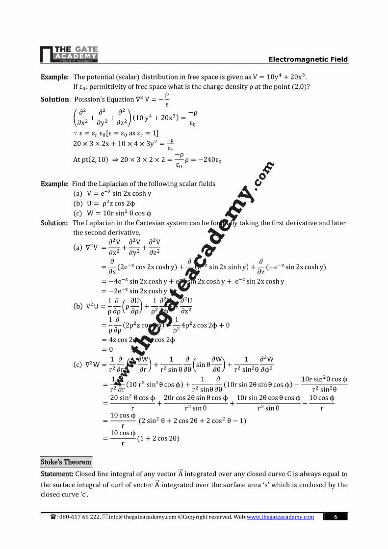
Stoke’s Theorem
Statement: Closed line integral of any vector A integrated over any closed curve C is always equal to
the surface integral of curl of vector A integrated over the surface area ‘s’ which is enclosed by the
closed curve ‘c’.
Electromagnetic Field
: 080-617 66 222, [email protected] ©Copyright reserved. Web:www.thegateacademy.com 7
∮ A . dL = ∫ ∫(∇ × A )
S
dS
The theorem is valid irrespective of
(i) Shape of closed curve ‘C’
(ii) Type of vector ‘A’
(iii) Type of co-ordinate system
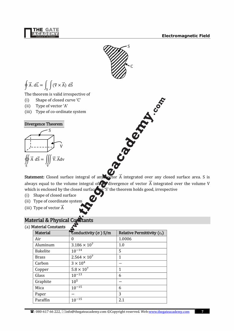
Divergence Theorem
∯A
S
dS = ∭V . A dv
V
Statement: Closed surface integral of any vector A integrated over any closed surface area. S is
always equal to the volume integral of the divergence of vector A integrated over the volume V
which is enclosed by the closed surface are ‘S’ the theorem holds good, irrespective
(i) Shape of closed surface
(ii) Type of coordinate system
(iii) Type of vector A
Material & Physical Constants (a) Material Constants
Material Conductivity (σ ) S/m Relative Permittivity (εr)
Air 0 1.0006
Aluminum 3.186 × 10⁷ 1.0
Bakelite 10−14 5
Brass 2.564 × 10⁷ 1
Carbon 3 × 10⁴ −
Copper 5.8 × 10⁷ 1
Glass 10−13 6
Graphite 105 −
Mica 10−15 6
Paper − 3
Paraffin 10−15 2.1
S
V
S
C