efï¬cient enumeration of phylogenetically informative substrings

JOURNAL OF COMPUTATIONAL BIOLOGY

Volume 14, Number 6, 2007

© Mary Ann Liebert, Inc.

Pp. 701–723

DOI: 10.1089/cmb.2007.R011

Efficient Enumeration of Phylogenetically

Informative Substrings

STANISLAV ANGELOV,1 BOULOS HARB,1 SAMPATH KANNAN,1

SANJEEV KHANNA,1 and JUNHYONG KIM2

ABSTRACT

We study the problem of enumerating substrings that are common amongst genomes thatshare evolutionary descent. For example, one might want to enumerate all identical (there-fore conserved) substrings that are shared between all mammals and not found in non-mammals. Such collection of substrings may be used to identify conserved subsequencesor to construct sets of identifying substrings for branches of a phylogenetic tree. For twodisjoint sets of genomes on a phylogenetic tree, a substring is called a tag if it is found in allof the genomes of one set and none of the genomes of the other set. We present a near-lineartime algorithm that finds all tags in a given phylogeny; and a sublinear space algorithm (atthe expense of running time) that is more suited for very large data sets. Under a stochasticmodel of evolution, we show that a simple process of tag-generation essentially capturesall possible ways of generating tags. We use this insight to develop a faster tag discoveryalgorithm with a small chance of error. However, since tags are not guaranteed to exist in agiven data set, we generalize the notion of a tag from a single substring to a set of substrings.We present a linear programming-based approach for finding approximate generalized tagsets. Finally, we use our tag enumeration algorithm to analyze a phylogeny containing 57

whole microbial genomes. We find tags for all nodes in the phylogeny except the root forwhich we find generalized tag sets.

Key words: design and analysis of algorithms, phylogenetically informative substring, phylogeny,stochastic analysis, suffix tree.

1. INTRODUCTION

GENOMES ARE RELATED to each other by evolutionary descent. Thus, two genomes share sequenceidentities in regions that have not experienced mutational changes; i.e., the genomes share common

subsequences. While common subsequences can also arise by chance, sufficiently long common sequencesare homologous (identity by descent) with high probability. The pattern of common subsequences in a set of

1Department of Computer and Information Science, University of Pennsylvania, Philadelphia, Pennsylvania.2Department of Biology, University of Pennsylvania, Philadelphia, Pennsylvania.

701

702 ANGELOV ET AL.

genomes can be informative for reconstructing the evolutionary history of the genomes. Furthermore, sincestabilizing selection for important functions can suppress fixed mutational differences between genomes,long common subsequences can be indicative of important biological function. This hypothesis has beenextensively used in comparative genomics to scan genomes for novel putatively functional sequences(Bejerano et al., 2004, 2005; Siepel et al., 2005).

Typical approaches for obtaining such subsequences involve extensive pairwise comparison of sequencesusing BLAST-like approaches along with additional modifications. Alternatively, one can use a dictionary-based approach, scanning the genomes for presence of common k-mers (which is also the base approachfor BLAST heuristics). The presence and absence of such k-mers can be also used to identify unlabeledgenomes or reconstruct the evolutionary history. Detection of particular k-mers can be experimentallyimplemented using oligonucleotide microarrays leading to a laboratory genome identification device.

For detecting functionally important common subsequences or for identifying unlabeled genomes, it isimportant that k is sufficiently large to ensure homologous presence with high probability. However, therequired address space increases exponentially with k. Furthermore, not all patterns of k-mer presence areinformative for detecting common subsequences. If the phylogenetic relationship of the genomes is known,then the phylogeny can become a guide to delineating the most informative common subsequences. Forany given branch of the tree, there will be substrings common to all genomes on one side of the branchand not present on the other side. For example, there will be a collection of common substrings uniqueto the mammalian lineage of the Vertebrates. Such substrings will be parts of larger subsequences that areconserved in the mammalian genomes; and, such substrings will be indicators of mammalian genomes.If we had an enumeration of all such informative common substrings, we can apply the information toefficiently detect conserved subsequences or to an experimental detection protocol to identify unlabeledgenomes. In this paper, we describe a procedure to efficiently enumerate all such informative commonsubstrings (which we call “sequence tags”) with respect to a guide phylogeny. In particular, here we explorethe application to the construction of an identification oligonucleotide detection array, which can be appliedto high-throughput genome identification and reconstructing the tree of life.

More specifically, given complete genomes for a set of organisms S and the binary phylogenetic treethat describes their evolution, we would like to be able to detect all discriminating oligo tags. We will saythat a substring t is discriminating at some node u of the phylogeny if all genomes under one branch of ucontain t while none of the genomes under any other branch of u contains t . Thus, a set of discriminatingtags, or simply tags, for all the nodes of a phylogeny allows us to place a genome that is not necessarily

sequenced in the phylogeny by a series of binary decisions starting from the root. This procedure canbe implemented experimentally as a microarray hybridization assay, enabling a rapid determination ofthe position of an unidentified organism in a predetermined phylogeny or classification. It is noteworthythat heuristic construction of short sequence tags has been used before for identification and classification(Amann and Ludwig, 2000), but no algorithm has been presented for data driven tag design.

Our results

! We first present an efficient algorithm for enumerating substrings common to the extant sequences underevery node of a given phylogeny. The algorithm runs in linear time and space.

! We use our common-substrings algorithm to develop a near-linear time algorithm for generating thediscriminating substrings for every node of the phylogeny. Specifically, if S is the set of given genomes,the discriminating-substrings algorithm runs in time O.njS j log jS j/ where n is the average length ofthe genomes. This improves the analysis of Angelov et al. (2006) and an earlier bound of O.njS j2/given in Angelov et al. (2004).

! Even though all the above algorithms require linear space, due to physical memory limitations theymay be impractical for analyzing very large genomic data sets. We therefore give a sublinear spacealgorithm for finding all discriminating substrings (or all common substrings). The space complexity ofthe algorithm is O.n=d/ and its running time is O.dnjS j2/ assuming each genome size is O.n/. Thetradeoff between the time and space complexities is controlled by the parameter d .

! We demonstrate the existence of tags in the prokaryotes data set of Wolf et al. (2002). The genomesrepresented in the data set span two of the three recognized domains of life. We find that either left orright tags exist for all nodes of the phylogeny except the root.

EFFICIENT ENUMERATION OF PHYLOGENETICALLY INFORMATIVE SUBSTRINGS 703

! Motivated by our results on the microbial genomes, we study the potential application to arbitrary scalephylogenetic problems using the Jukes-Cantor model of molecular evolution (Jukes and Cantor, 1969).We assume that the given species set S is generated according to this model. We first analyze the casewhere the phylogeny is a balanced binary tree with a uniform probability of change on all its edges. We

show that in this setting, if t is a tag that discriminates a set S 0 of species from set NS 0, then w.h.p. that

increases with the number of species—probability " 1= .1 C O.ln.n/=jS j//—t is present in the common

ancestor of S 0 (occurs early in the evolution) and is absent from the common ancestor of NS 0 (is absent

from the beginning). Our study of the stochastic model allows us to design faster algorithms for taggeneration with small error. Even when we allow arbitrary binary trees, we show that this probabilityis " 1=2.

! As observed in our experiments and subsequent analysis, tags are not guaranteed to exist in a givendata set. We consider a relaxed notion of tags to deal with such a scenario. Given a partition .S 0; NS 0/ ofspecies, we say that a set T of tags is an .˛; ˇ/-generalized tag set for some ˛ > ˇ, if every species in S 0

contains at least an ˛ fraction of the strings in T and every species in NS 0 contains at most a ˇ fraction ofthem. Clearly, such a tag set can still be used to decide whether a genome belongs to S 0 or to NS 0. We showthat the problem of computing generalized tag sets may be viewed as a set cover problem with certain“coverage” constraints. We also show that this generalization of tags is both NP-hard and LOGSNP–hardwhen .˛; ˇ/ D .2

3; 1

3/. However, if jT j D !.log m/, a simple linear programming based approach can

be used to compute approximate generalized tag sets. As an example, we find .23; 1

3/-generalized tag

sets for the root of the prokaryotes phylogeny (where we did not find tags).

2. PRELIMINARIES

Formally, the problems we consider are the following:

Hierarchical common substring problem (HCS)

Input: A set of strings S D fs1; : : : ; smg drawn from a bounded-size alphabet with total lengthPm

iD1 jsi j # nm, where n denotes the average length of the strings; and an m-leaf binary tree P whoseleaves are labeled s1; : : : ; sm sequentially from left to right.

Goal: For all u 2 P , find the set of (right-)maximal substrings common to the strings in Su, where Su

is the set of all the input strings in the subtree rooted at u.

A substring t common to a set of strings is right-maximal if for any non-empty string ˛, t˛ is no longera common substring, i.e., t is not a proper prefix of a common substring. The substring t is maximalif it is not a substring of another common substring. Given a set of strings, (right-)maximal commonsubstrings compactly encode all common substrings. Here, we focus on finding right-maximal commonsubstrings. The obtained result generalizes to maximal substrings in a straightforward manner (Gusfield,1997; Angelov et al., 2004).

Discriminating substrings. A substring t is said to be a discriminating substring or a tag for a nodeu in a phylogeny if all strings under one branch of u contain t while none of the strings under the otherbranch contain t . The input to the discriminating substring problem is the same as that for the first problem.

Discriminating substring problem

Input: A set of strings S and a binary tree P .Goal: Find sets Du for all nodes u 2 P , such that Du contains all discriminating substrings for u.

We will also need the notion of a generalized tag set.

.˛; ˇ/-generalized tag set. Given a partition .S 0; NS 0/ of species, we say that a set T of tags is an.˛; ˇ/-generalized tag set for some ˛ > ˇ, if every species in S 0 contains at least an ˛ fraction of thestrings in T and every species in NS 0 contains at most a ˇ fraction of them.

704 ANGELOV ET AL.

Suffix trees. Suffix trees, introduced in Weiner (1973), play a central role in our algorithms. A suffixtree T of a string s is a trie-like data structure that represents all suffixes of s. We adopt the followingdefinitions from Gusfield (1997). The path-label of a node v in T is the string formed by following thepath from the root to v. The path-labels of the jsj leaves of T spell out the suffixes of s, and the path-labelsof internal nodes spell out substrings of s. Furthermore, the suffix tree ensures that there is a unique pathfrom the root, not necessarily ending at an internal node, that represents each substring of s. We also saythat the path-label of node v is the string corresponding to v in the tree.

The algorithms we present are based on generalized suffix trees (Gusfield, 1997). A generalized suffixtree extends the idea of a suffix tree for a string to a suffix tree for a set of strings. Conceptually, it canbe built by appending a unique terminating marker to each string, then concatenating all the strings andbuilding a suffix tree for the resultant string. The tree is post-processed so that each path-label of a leaf inthe tree spells a suffix of one of the strings in the set and, hence, is terminated with that string’s uniquemarker.

Proposition 1 (McCreight, 1976; Ukkonen, 1995). Given a string of length n drawn from a bounded-

size alphabet, we can construct its suffix tree in O.n/ time and space.

3. THE HIERARCHICAL COMMON SUBSTRING PROBLEM

Long common substrings among genomes can be indicative of important biological functions. In thissection we give a linear time/linear space algorithm that enumerates substrings common to all sequencesunder every node of a given binary phylogeny. This is a significant improvement over naively running thelinear time common substrings algorithm of Hui (1992) for every node of the phylogeny. By carefullymerging sets of common substrings along the nodes of the phylogeny and eliminating redundancies weare able to achieve the desired running time. Note that for a given node, there may be quadratically manysubstrings common to its child sequences. The algorithm will therefore list all right-maximal commonsubstrings. Such substrings efficiently encode all common substrings. The formal problem description isgiven in Section 2. We start with two definitions.

Definition 1. Let C be a collection of nodes of a suffix tree. A node p 2 C is said to be redundant if

its path-label is empty or it is the prefix of some other node in C .

Definition 2. For a tree T , let o.v/ be the postorder index of node v 2 T .

Algorithm HCS. We preprocess the input as follows: (a) Build a generalized suffix tree T for thestrings in S by using two copies of every si 2 S , each with a unique terminating marker: s1#1a s1#1b

! ! !sm#masm#mb

; (b) Process T so that lowest common ancestor (lca) queries can be answered in constanttime; and, (c) Label the nodes of T with their postorder index.

1. For each node u 2 P , build a list Cu of nodes in T with the following properties:(P1) A substring t is common to the strings in Su if and only if t is a prefix of the path-label of a

node in Cu.(P2) The elements of Cu are sorted based on their postorder index.(P3) No element p of Cu is redundant.The lists are built bottom-up starting with the leaves of P :(a) For each leaf u 2 P , since jSuj D 1, compute Cu by removing the redundant suffixes of s 2 Su.(b) For each internal node u 2 P , let l.u/ and r.u/ be the left and right children of u respectively.

We compute Cu D Cl.u/ u Cr.u/, where

A u B D fp D lca.a; b/ W a 2 A; b 2 B; p not redundantg :

2. For each u 2 P , output Cu.


Analysis. The time and space complexities of the preprocessing phase are O.nm/ (see Proposition 1)(Harel and Tarjan, 1984; Schieber and Vishkin, 1988). We note that the tree T is obtained by concatenatingtwo copies of each input string terminated with different end markers. This ensures that each suffix ofan input string terminates at an internal node of T and simplifies our presentation. The construction isonly conceptual and the above property can be emulated using the standard generalized suffix tree methodwhere each string appears only once.

We now analyze Step 1. The lists Cu for the leaves of P are first simultaneously built in Step 1(a) byperforming a postorder walk on T . Assuming Su D fsi g, node p ¤ root.T / is appended to list Cu if ithas an outgoing edge labeled “#ia .” Suffix tree properties guarantee that Cu will consist of all of the jsi jsuffixes of si . Since the list was constructed via a postorder walk on T , it will also possess P2. PropertyP3 is obtained by scanning each list from left to right and removing redundant nodes. Observe that if pis an ancestor of q, then p is an ancestor of all q0 satisfying o.q/ ! o.q0/ ! o.p/. Hence, we can removeredundancies from each Cu in time linear in jsi j by examining only adjacent entries in the list. Since everysubstring of si is a prefix of some suffix of si , and we removed only redundant suffixes, Cu possesses P1.We obtain the following lemma.

Lemma 1. Cu possesses properties P1, P2, and P3 for each leaf u 2 P .

We now show how to compute the lists Cu for the internal nodes of P . We first show that the operationu as defined in Step 1(b) preserves P1.

Lemma 2. Let u 2 P be the parent of l.u/ and r.u/. If Cl.u/ and Cr.u/ possess P1, then Cu DCl.u/ u Cr.u/ also possesses P1.

Proof. The string t is a common substring to the strings in Su if and only if t is common to the stringsin Sl.u/ and Sr.u/. This is equivalent to the existence of p 2 Cl.u/ and q 2 Cr.u/ such that t is a prefix ofthe path-labels of both p and q. That is, t is a prefix of the path-label of lca.p; q/ as required.

For each internal node u 2 P , we construct a merged sorted list Yu containing all the elements of Cl.u/

and Cr.u/ with repetitions. Let src.a/ be the source list of node a 2 Yu. When computing Cl.u/ u Cr.u/,the following lemma allows us to only consider the lca of consecutive nodes in Yu whose sources aredifferent.

Lemma 3. If a; a0; b; b0 2 T satisfy o.a0/ ! o.a/ ! o.b/ ! o.b0/, then lca.a0; b0/ is an ancestor of

lca.a; b/.

Proof. By postorder properties, lca.a0; b0/ is an ancestor of both a and b so it is an ancestor oflca.a; b/.

Let a; a0; b; b0 2 Yu, where o.a0/ ! o.a/ ! o.b/ ! o.b0/. If src.a/ ¤ src.b/ and src.a0/ ¤ src.b0/, then,since lca.a0; b0/ is an ancestor of lca.a; b/, the former is redundant. This suggests the following procedurefor computing the list Cu starting from the empty list. Suppose at step i 2 f1; : : : ; jYuj " 1g, a D YuŒi !and b D YuŒi C 1!: If src.a/ D src.b/, proceed to next step; else, let p0 D lca.a; b/. If p0 D root.T / thenwe discard it and proceed to the next step. In order to avoid redundancies before appending p0 to Cu, wecompute lca.p; p0/ where p is the last node appended to Cu. If lca.p; p0/ D p0 we discard p0, and iflca.p; p0/ D p we replace p with p0.

Each step of the above procedure requires constant time. Hence, since jYuj ! jCl.u/j C jCr.u/j, theprocedure runs in O.jCl.u/j C jCr.u/j/ time. The next lemma shows the correctness of the procedure.

Lemma 4. For an internal node u 2 P , the above procedure correctly computes Cu D Cl.u/ u Cr.u/.

Furthermore, the list Cu is sorted and jCuj ! minfjCl.u/j; jCr.u/jg.

706 ANGELOV ET AL.

Proof. Since the above procedure performs all necessary lca computations, we only need to show thatit maintains P2 and P3 for the resulting list. The proof for properties P2 and P3 proceeds by induction onthe steps of the procedure. Let u be an internal node of P . After the first step, jCuj ! 1, and Cu triviallypossesses P2 and P3. Now assume that the two properties are maintained for all i < k. We prove that theyalso hold for i D k. Let p be the last node appended to Cu, and let p0 be the newly computed node. Notethat, by the inductive hypothesis, o.p/ " o.q/, 8q 2 Cu. We proceed by cases.

1. o.p0/ " o.p/ and p0 is an ancestor of p. Then, p0 is redundant and we do not append to Cu.2. o.p0/ > o.p/ and p0 is not an ancestor of p. Then, by appending p0 to Cu, Cu remains sorted and

none of the nodes in Cu will be redundant. Assume, for contradiction, there is a node q such thato.q/ < o.p/ and p0 is an ancestor of q. Then p0 is also an ancestor of p; a contradiction.

3. o.p0/ < o.p/ and p is an ancestor of p0. Then, p is redundant and is removed from the list. We nowshow that Cu will remain sorted after adding p0. Assume it is not. Then, there exists q 2 Cu such thato.p0/ < o.q/ < o.p/. It follows that p is also an ancestor of q; a contradiction. Finally, since p0 isdescendant of p, by the inductive hypothesis, it cannot be an ancestor of any other node in Cu.

4. o.p0/ < o.p/ and p is not an ancestor of p0. This case is impossible. Assume o.p0/ < o.p/ and p isnot an ancestor of p0, and let p D lca.a; b/ and p0 D lca.a0; b0/ where a; a0; b; b0 2 Yu. Since p0 isgenerated at a later stage than p, it follows that o.p/ > o.p0/ " maxfo.a0/; o.b0/g " maxfo.a/; o.b/g.But then p is an ancestor of p0; a contradiction.

Finally, jCuj ! jCl.u/j since !q; q0 2 Cu, q ¤ q0 where q and q0 are ancestors of the same node inCl.u/. If they were, one would be redundant. Since P3 ensures that Cu has no redundant nodes, we havethat jCuj ! jCl.u/j. Similarly, we have jCuj ! jCr.u/j.

We are now ready to state the following theorem.

Theorem 1. The Hierarchical Common Substring Problem can be solved in O.nm/ time and O.nm/space.

Proof. The correctness of the algorithm follows from Lemmas 1, 2, 3, and 4. The time and spacerequirements for Step 1(a) are bounded by O.nm/ C

P

jsi j D O.nm/ since to compute all lists Cu

when u is a leaf of P we need to walk T once, and postprocess each list in time proportional to jsi j.For Step 1(b), we need time and space proportional to

P

internal u jCuj. From Lemma 4, we have jCuj !minfjCl.u/j; jCr.u/jg for all internal nodes u 2 P . Hence, jCuj ! jCvj where v is the rightmost leaf of u’sleft subtree; therefore since each leaf node accounts for at most one internal node,

X

internal u

jCuj !X

leaf v

jCvj ! nm:

The theorem follows.

4. THE DISCRIMINATING SUBSTRING PROBLEM

In this section, we will use the phylogeny for extracting the most informative substrings common to thechild sequences of every node in the phylogeny. Suppose we know that a sequence belongs to a certainsubtree of the phylogeny that is rooted at u. We wish to know whether the sequence belongs to the left orright branch of u. If we knew the substrings common to the left subtree of u but not present in the rightsubtree (or vice versa), then we would know to which of the two subtrees the sequence belongs. Hence fora given node, the substrings that are common to its children but not present in the children of its siblingare more informative than only the common ones. Below we show two methods with certain tradeoffs forfinding such discriminating substrings or tags, for every node in the phylogeny. It is easy to see that the setof tags obtained by selecting a tag from each node on a root-leaf path uniquely distinguishes the sequence

at the leaf from all other sequences in the phylogeny.


4.1. A near-linear time algorithm

The HCS algorithm finds all common substrings for each node in P . The common substrings are encodedas the prefixes of the path-labels of the nodes in Cu for each u 2 P . However, these substrings may notbe discriminating. That is, the prefix of the path-label of a node p 2 Cl.u/ (symmetrically Cr.u/) may alsobe a substring of one of the strings in Sr.u/ (Sl.u/). The following algorithm finds for each node in Cl.u/

its longest path-label prefix that is not discriminating.

Algorithm. Let Cu for all u 2 P be the output of the HCS algorithm and let T be the computed suffixtree.

1. For each u 2 P , build a list Au of nodes in T with the following properties:(P4) A string t is a substring of a string in Su if and only if t is a prefix of the path-label of a node

in Au.(P5) The elements of Au are sorted based on their postorder index.The lists are built bottom-up starting from the leaves of P :(a) For each leaf node u 2 P , Au D Cu.(b) For each internal node u 2 P n froot.P /g, compute Au D Al.u/ [ Ar.u/.

2. For each internal node u 2 P , compute the set of discriminating substrings encoded with Du, where,

Du D

(

.p; w/ W p 2 Cl.u/; o.p/ < o.w/; w D lca

p; arg minq2Ar.u/

Œo.lca.p; q//!

!)

:

In the above expression for Du, w is the node in the suffix tree whose path-label is the longest properprefix of the path-label of p that is present in some string in the right subtree of u. For all q 2 Ar.u/,arg minq2Ar.u/

Œo.lca.p; q//! finds the q that has the deepest lowest common ancestor with p, i.e., the qwhose path-label shares the longest prefix with that of p. The condition o.p/ < o.w/ guarantees that theleast common ancestor found is a proper ancestor to p.

Analysis. We first show how each Du encodes all discriminating substrings for u 2 P .

Lemma 5. A string t is discriminating for an internal node u 2 P if and only if 9.p; w/ 2 Du such

that the path-label of w is a proper prefix of t and t is a prefix of the path-label of p.

Proof. (if) Let .p; w/ 2 Du, and suppose t is a string such that the path-label of w is a proper prefixof t and t is a prefix of the path-label of p. By P1, t is a common substring of the strings in Sl.u/. Assumefor contradiction that t is a substring of some string in Sr.u/. Then, by P4, 9q 2 Ar.u/ such that t is aprefix of the path-label of q. But then, since w is a proper prefix of t , it is a proper prefix of the path-labelsof both p and q. Hence, o.w/ > o.lca.p; q//; a contradiction.

(only-if) Suppose t is a discriminating string for u. Then, 9p 2 Cl.u/ such that t is a prefix of thepath-label of p, and, by P4, !q 2 Ar .u/ such that t is a prefix of the path-label of q. Hence, the path-label

of w D lca!

p; arg minq2Ar.u/Œo.lca.p; q//!

"

is a proper prefix of t .

The next corollary, following from the definition of Du and Lemma 3, will allow us to efficientlycompute w as defined in Du for a given p 2 Cl.u/.

Corollary 1. Given p 2 Cl.u/ . Let q0; q00 2 Ar.u/ be such that

q0 D arg maxq2Ar.u/Wo.q/!o.p/

Œo.q/!; q00 D arg minq2Ar.u/Wo.q/>o.p/

Œo.q/!:

If there is no such q0 (resp. q00), we set q0 D q00 (resp. q00 D q0). Let

w D arg minq2flca.q0;p/;lca.q00;p/g

Œo.q/!:

Then, .p; w/ 2 Du if and only if o.p/ < o.w/, or equivalently, lca.q0; p/ ¤ p.

708 ANGELOV ET AL.

We next show how to compute the lists Au for the internal nodes of P . Note that for a leaf u 2 P ,since jSuj D 1 and Cu is sorted, Au D Cu trivially possesses both P4 and P5. Furthermore, for an internalnode u 2 P , the union operation maintains P4. Now merging two sorted lists of sizes N and M , withM ! N , requires at least dlog

!

NCMN

"

e D ‚.M log NM

/ comparisons to distinguish among the!

NCMN

"

possible placements of the elements of the larger list in the output. We can use the results of Brown andTarjan (1980, 1979) and Pugh (1990), for example, to match this lower bound. The analysis assumes thatthe Au lists are represented as linked-level 2-3 trees (Brown and Tarjan, 1980). Conversion of these liststo 2-3 trees for the leaves is direct since they are sorted.

Lemma 6. The lists Au, for all u 2 P , can be computed in O.nm log m/ time.

Proof. For the purpose of analysis we assume that the elements in the sets Au for the leaf nodes ofP are all distinct, i.e., jAroot.P /j D

P

leaf u jAuj D O.nm/. Therefore these elements define an universe ofelements, call it U , and Au " U , for all u 2 P . Furthermore, note that an element a 2 Au, where u is aleaf of P , occurs only in lists Av , where v is an ancestor of u.

Given an internal node u 2 P , let Su (resp. Lu) be the smaller (resp. larger) list of Al.u/ and Ar.u/

breaking ties arbitrarily and define xu D jLuj=jSuj. Since at each internal node, we merge the smaller list(Su) into the larger one (Lu), the running time to compute the lists Au’s is proportional to

X

internal u

jSuj logxu:

We obtain a bound on the above quantity in terms of n and m by bounding the contribution of eachelement of U to the running time. That is, consider an element a 2 U —for each node u such that a 2 Su,we can charge the element a, O.log xu/ credits to the running time. We compute the total charge to allelements of U as follows.

Given a leaf node u 2 P , let Xu be the set of ancestral nodes of u in P such that Au " Sv and jSvj # nfor all v 2 Xu. (Note that the size of Sv only increases as the distance between v and root.P / decreases.)Let w 2 Xu be the closest node to u. Since jAvj # jSvj.xv C 1/ # jSvjxv, we have jSw j

Q

v2Xuxv !

jAroot.P /j ! nm; henceQ

v2Xuxv ! m. Therefore, the contribution of each element a 2 Au to the running

time with respect to Xu is proportional to

X

v2Xu

log xv D log

0

@

Y

v2Xu

xv

1

A ! log m:

Therefore, each element a 2 U contributes at most O.log m/ to the running time of all merges wherejSuj # n. Since jU j D O.nm/, the total contribution is O.nm log m/.

Now, consider a node u where jSuj < n. Since jLuj ! nm, it takes O.jSuj log nmjSuj

/ D O.n log m/ timeto compute the list Au. Since there are at most m $ 1 internal nodes, the total contribution of such mergesto the running time is O.nm log m/. The lemma follows.

Now, we can compute Du for an internal node u 2 P by finding the position of each p 2 Cl.u/ in thesorted Ar.u/, determining its immediate neighbors q0 and q00, and computing w as in Corollary 1. If weconsider the elements of Cl.u/ in their sorted order, then by Brown and Tarjan (1980), and since jAr.u/j DO.nm/, finding the positions of all the elements of Cl.u/ in Ar.u/ takes O

!

jCl.u/j log.nm=jCl.u/ j/"

time.Moreover, finding the neighbors of each one of these elements takes constant time. This leads to thefollowing lemma.

Lemma 7. Given the lists Au, for all nodes u 2 P , the lists Du, for all internal nodes u 2 P , can be

computed in O.nm log m/ time.

Proof. The running time to compute the lists Du, for all internal nodes u 2 P , is proportional to

X

internal u

jCl.u/j log.nm=jCl.u/ j/:


From the proof of Theorem 1, we have thatP

internal u jCl.u/j !P

u2P jCuj D O.nm/. The runningtime is maximized when all of the m"1 lists Cl.u/ are as large as possible and have equal sizes. Therefore,setting jCl.u/j D O.n/ we obtain the stated running time.

Note that we can simultaneously compute the lists Cu, Au, and Du, for each internal node u 2 P ,in a bottom-up fashion discarding Al.u/ and Ar.u/ at the end of the computation for each u. Hence, thetotal size of the Au lists we store at any point is no more than

P

leaf v Av D O.nm/. Finally, since, bydefinition, jDuj ! jCl.u/j, the space required to store Cu and Du for all u 2 P is O.nm/. We, therefore,obtain the following theorem.

Theorem 2. The Discriminating Substring Problem can be solved in O.nm log m/ time and O.nm/space.

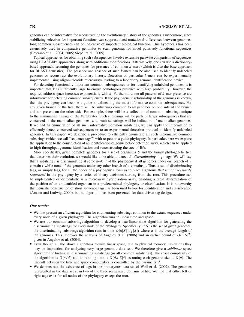
Example. We illustrate the HCS algorithm and the discriminating substring algorithm presented in theprevious sections through a concrete example. Consider the phylogeny P and the set of strings S givenin Figure 1a. The generalized suffix tree T obtained in the preprocessing phase of the HCS algorithm isgiven in Figure 1b. Recall that the tree T has the property that every suffix of an input string terminatesat an internal node of T .

We first describe how the lists Cv in step 1 of the HCS algorithm are computed for all nodes v 2 P .For the leaf nodes, we have C1 D f1; 7; 12; 15g, C2 D f2; 8; 13g, and C3 D f4; 9; 10; 14g. These lists arecomposed of indices from the suffix tree that encode the non-redundant suffixes of strings s1, s2, and s3

respectively. Note that node 6 is not in C2 because it is an ancestor (prefix) of node 2 and therefore itis redundant. To obtain Cu D C1 u C2, we first compute the union Yu of C1 and C2 maintaining thesource of each element: Yu D f1; 2; 7; 8; 12; 13; 15g; here, underlined elements have C2 as a source list.Scanning Yu from left to right, we consider adjacent elements with different source lists and their lowestcommon ancestors: lca.1; 2/ D 3, lca.2; 7/ D 16, lca.7; 8/ D 9, lca.8; 12/ D 16, lca.12; 13/ D 14, andlca.13; 15/ D 16. We obtain Cu D f3; 9; 14g by removing redundancies (none in this case) and the rootof the suffix tree (which represents the empty string). The list Cu encodes the common substrings of s1

and s2; i.e., the strings ACG, CG, G, and all of their proper prefixes: AC, A, and C. Similarly, we haveYr D f3; 4; 9; 9; 10; 14; 14g and Cr D f5; 9; 14g.

The discriminating substrings algorithm then prunes the set of common substrings for each node asfollows. In step 1, the algorithm computes the lists Av for all nodes v 2 P n frg. We have A1 D C1,

FIG. 1. An example phylogeny P with extant species S D fs1; s2; s3g, and their corresponding generalized suffixtree. (a) The phylogeny P whose leaf nodes are associated with the strings s1 D ACGT, s2 D ACGA, and s3 D ACCG.

Leaf nodes are labeled with 1, 2, and 3, and the internal nodes with u and r (the root). (b) The generalized suffix

tree T for the strings s1, s2, and s3 constructed from s1#1as1#1bs2#2as2#2b

s3#3a s3#3b. Leaf nodes (with incoming

edges labeled #1a ; #1b; #2a ; #2b

; #3a ; #3b) are omitted for clarity of presentation. Internal nodes are labeled with their

postorder index. The index of the root node is 16.

710 ANGELOV ET AL.

A2 D C2, A3 D C3, and Au D C1 [ C2. To reduce the space requirement, once Au is computed, lists A1

and A2 are discarded. Now to compute the discriminating substrings for, say, node r , we need to prune Cu

using A3 to obtain the left tags, and we need to prune C3 using Au to obtain the right tags. The calculationsfor the left tags are as follows. For each element of Cu we efficiently find its immediate neighbors in A3.For node 3, the neighbor is 4; for node 9, the neighbors are 9 and 10; for node 14, the neighbor is 14.Applying the calculations in Corollary 1, we obtain Du D f.3; 5/g. The pair .3; 5/ encodes all prefixes ofACG (node 3) that are longer than AC (node 5); i.e., it identifies the single discriminating tag ACG.

4.2. A sublinear space algorithm

The above algorithms are optimal or near optimal in terms of their running times and they require onlylinear space. For very large genomes, even linear space might not fit in primary memory. It is important tofurther reduce the algorithms’ space requirements for such situations to avoid expensive access to secondarystorage. Intuitively, it seems that we should be able to run the algorithms on chunks of the data at a timein order to reduce the space complexity. Below we describe such a sublinear space algorithm, with a time-space tradeoff, for finding all discriminating substrings (or all common substrings). The precise tradeoffis stated in Theorem 3. The running time of the algorithm will also depend on the underlying structureof the input phylogeny, specifically its height. Recall that the height of a tree P is equal to the maximumnumber of edges on a simple root-leaf path.

In this section, we assume that the maximum genome length is O.n/ where n is the average genomelength. Such an assumption is reasonable when dealing with genome data from relatively close species.When this condition does not hold, the running time of the stated algorithm increases by an additionalfactor proportional to the ratio of the maximum to average genome length in the input.

Algorithm outline and analysis. The algorithm proceeds by considering each node of the phylogenyP independently. For a node u 2 P , we can find the set of discriminating substrings Du by using thematching statistics algorithm introduced in Chang and Lawler (1994). Given strings s and s0, the algorithmcomputes the length m.s; j; s0/ of the longest substring of s starting at position j in s and matching somesubstring of s0. This is done by first constructing the suffix tree for s0 and then walking the tree using s.The algorithm requires O.js0j/ time and space for the construction of the suffix tree, and O.jsj/ additionaltime and space to compute and store m.s; j; s0/ for all j .

Let Su be the union of two disjoint sets Lu and Ru D SunLu where Lu and Ru are the sets of stringsunder the two branches of u 2 P . A substring starting at position j of s 2 Lu is discriminating for u ifand only if

mins02Lu

m.s; j; s0/ ! maxs02Ru

m.s; j; s0/ > 0: (1)

That is, there exists a substring of s starting at j that is common to all strings in Lu and is sufficientlylong so that it does not occur in any string in Ru. If a position j satisfies (1), then a substring t startingat j such that maxs02Ru m.s; j; s0/ < jt j " mins02Lu m.s; j; s0/ is discriminating. Clearly, all tags aresubstrings of s and thus the outlined procedure computes Du. The running time of the algorithm isP

s02SuO.jsj C js0j/ D O.nm/ and requires O.maxs02Su js0j/ D O.n/ space. Computing the set of tags

for all nodes of P with tree height h requires O.nmh/ time and O.n/ space matching the running time ofAngelov et al. (2004). By limiting the maximum allowed length of a tag, we can obtain a tradeoff betweenthe running time and memory required by the algorithm as stated in the following theorem.

Theorem 3. The Discriminating Substring Problem for tags of length O.n=d/, for some threshold

parameter d , 1 " d " n, can be solved in time O.dnmh/ and O.n=d/ space, where h is the height of P .

Proof. We will show the required modifications to the above algorithm in order to include the desiredtime-space tradeoff parameter d . Given the length of tags of interest is at most n=d , the algorithm can beadapted to use O.n=d/ memory and O.dnm/ time to compute the set of all discriminating tags Du for anode u of P by virtually chopping each input string in O.d/ overlapping segments of length 2n=d . Fora string s 2 Su and an integer i 2 Œ0; jsj=d/, let s.i/ denote the segment that starts at position n

di C 1.


Note that the overlap between consecutive segments s.i/ and s.i C 1/ ensures that each substring of swith length at most n=d is contained in some segment. Since tags must occur in all strings in Lu, we picka representative string s 2 Lu and find tags contained within each of its segments. For a segment s.i/,we can find all its discriminating tags by computing m.s.i/; j; s0/ D maxs0.k/ m.s.i/; j; s0.k// instead ofm.s; j; s0/ in expression (1) above. Computing m.s.i/; j; s0/ for all positions j in s.i/ takes O.n/ time sincethere are O.d/ segments in each string s0 each with length O.n=d/. This implies that the computation ofexpression (1) for each s.i/ takes O.nm/ time as there are O.m/ strings in Lu and Ru. Once we processthe current segment of s and produce the tags that are contained within it, we add that segment to the setRu to avoid generation of duplicate tags. We then repeat the procedure for the remaining segments of s.The total running time per node is then O.dnm/ as, again, there are O.d/ segments in s.

Since we need to process only two segments at a time, we need only O.n=d/ space.

Remark. Since a tag may occur more than once in a segment, we can further eliminate duplicatesby maintaining the relevant matching statistics information at the nodes of the suffix tree for the currentsegment. Then, non-redundant tags can then be output in a bottom-up fashion. Note that the generalizedsuffix tree of two strings can be obtained by augmenting the suffix tree of the first sequence (Ukkonen,1995). This allows for quickly identifying the correspondence between the nodes of the two trees. Therefore,the modification does not affect the asymptotic time and space requirements.

5. DISCRIMINATING TAGS UNDER A STOCHASTIC MODEL OF EVOLUTION

We now analyze statistical properties of tags using a simplified assumption of molecular evolution.We make the first steps toward understanding the capability of tags to place new sequences in a givenphylogeny and their application to arbitrary scale phylogenetic problems. We show that there is a primary

mechanism for generating tags which suggests that tags are indicative of shared evolutionary history.We use the Jukes-Cantor model (Jukes and Cantor, 1969) for our analysis. In this model each position

in the genome evolves independently according to an identical stochastic process where the probability ofa mutation occurring per unit time is given by a parameter !. Further, it is assumed that the probability! of change is distributed equally between the 3 possible changes at a site. Thus if a site currentlyhas the nucleotide A, then it has probability !=3 of changing to C , for example, in unit time. Whenbranching occurs at a node in a phylogeny, then the two branches start with identical sequences but evolveindependently according to the stochastic process. Finally, we assume that the sequence at the root of thephylogeny is a random sequence of length n. Since we only allow substitutions all genomes will have thesame length. Given the actual time durations between evolutionary events, it is possible to represent theJukes-Cantor model by specifying the probabilities of change along each edge in the phylogeny wherethese probabilities depend on the time duration represented by the edge (e.g., if an edge is infinitely long,the probability of change is 3=4).

All of the current phylogeny models are some version of continuous time homogeneous Markov chainmodels. From an event point of view, these are all Poisson counting processes with event rates determined assome function of the model parameters and the different models only determining the marginal probabilityof state transitions. For our purposes the main determinants of the tags are where in the trees the events occurso the analysis on the Jukes-Cantor model should be reflective of the general cases.1 Even with this simplemodel, obtaining a closed-form representation of tag length distribution as a function of the probabilitiesof change along each edge is a complex task. We therefore start with a simplifying assumption—thephylogeny is a complete binary tree and the probability of change along each edge is p. We let h bethe height of our tree and label the sequences at its leaves with s1; : : : ; s2h . We label the sequence at theroot with r . We will focus on tags present in the left subtree of the root, which we call left tags. Similaranalysis holds for right tags and for other nodes in the tree. In Section 5.3, we generalize the analysis toarbitrary binary tree topologies and probabilities of change along the edges.

1Our simulation results can be reviewed at: www.cis.upenn.edu/!angelov/phylogeny/experiments/simulation/.

712 ANGELOV ET AL.

5.1. The primary mechanism for generating tags

Given the stochastic model of evolution we show that there is a dominant process by which tags aregenerated. We first prove that if the probability of change p along an edge is more than ln.n/=.2h!2k/,we do not expect tags to be generated. Using this bound on p, we show in Theorem 4 that the primarymechanism by which a tag t that discriminates a set S 0 of species from set NS 0 arises is one where t ispresent in the common ancestor of the species in S 0 and is absent from the common ancestor of thosein NS 0. In particular, if we let T denote the set of all tags and T 0 the set of tags generated by the primarymechanism, then we show that jT j ! jT 0j.1 C O. ln n

jS 0[ NS 0j//. Thus the error term decays inversely in the

number of species. We start with the following two lemmas bounding the minimum tag length and themaximum probability of change p.

Lemma 8. Tags have length greater than .1 " !/ log4 n w.h.p. where 0 < ! < 1.

Proof. Consider a sequence s in the right subtree of r . The sequence s is uniformly distributed since itevolved from a random sequence under the Jukes-Cantor model. Now let k ! .1 " !/ log4 n and considera k-mer t . If we partition s into strings of length k, then the probability that t does not appear in s

is at most .1 " 4!k/n=k ! e! n!

.1!!/ log4 n . Summing this probability over all possible k-mers, we get that

the probability some k-mer does not appear in s is upper bounded by e!n!

.1!!/ log4 n C.1!!/ ln n, which is

negligible.

Lemma 9. If p > 3 ln nk.2h!2/

, the expected number of tags of length k is < 1.

Proof. The left subtree has 2h!1 leaves. Consider the character at i th position of the leaf s1. Theprobability that a leaf sj , j ¤ 1, has the same character at position i is upper bounded by 1 " 2p=3. Theprobability that all leaves in the left subtree agree in the i th position is thus bounded by

.1 " 2p=3/k.2h!1!1/ ! exp."2pk.2h!1 " 1/=3/;

which is less than 1=n when p > 3 lnn=.k.2h " 2//.

Henceforth, we will assume that p ! 3 ln.n/=.k.2h " 2//. Let Ai for 1 ! i ! n " k C 1 be the eventthat position i in the root sequence, r , is good. Position i is said to be good if the k-mer starting at i inthe left child of r differs from that in the right child. Therefore, PrŒAi D 1" D 1 " .p2=3 C .1 " p/2/k .If the event Ai results in a tag being generated, we will say that this tag is a type–I tag. The followingtheorem shows that type–I tags are dominant.

Theorem 4. Let t be a sequence that either does not occur at the left child of the root or occurs at

the right child of the root. Then the probability that any such t is a left tag is negligible compared to theprobability of type–I tags.

Proof. Suppose that t is a left tag that appears in the i th position of all the sequences at the leaves ofthe root’s left subtree. Let tl and tr be the i th k-mers in the root’s left and right children respectively.

First, we will show that PrŒt D tl j t is a left tag"= PrŒt ¤ tl j t is a left tag" # 3=.8p/. We will assumethat when t ¤ tl , the two k-mers differ in exactly one position. (The above ratio only gets better if thenumber of differing positions is more than one.) Hence, independent of the value of the i th k-mer in theroot, PrŒt D tl "= PrŒt ¤ tl " # p=3.

The tag t can be generated by two processes, one starting with t D tl and the other starting with t ¤ tl .In the latter case, consider the position j that causes t to differ from tl , i.e., tl.j / ¤ t.j /. Let E be the setof maximal edges (closest to the root) such that for each edge e 2 E , the j th position becomes equal tot.j / for the first time at the node below e. Now let N.i/ be the number of ways of having such i maximalchanges. We know that N.2/ D 1 and N.3/ D 2. In general, N.i/ D 2N.i " 1/ C

Pi!2j D2 N.j /N.i " j /.


Hence, the probability that the j th position in every leaf is equal to t.j / is at mostP

i

!p3

"iN.i/. Note

that N.i C 1/ is the i th Catalan number Ci (see, for example, Stanley [1999]); therefore,

X

i

#p

3

$iN.i/ D

p

3

X

i

#p

3

$iCi ! 1

!

D1 !

p

1 ! 4p=3 ! 2p=3

2"

4p2

9:

The corresponding probability for the case when tl D t is lower bounded by .1 ! p/2h!2, which is theprobability of no changes in the left subtree to the j th position. Assuming t has length !.ln n/ and using

Lemma 9 we find that this lower bound is at least 1=2. Hence, the desired ratio is at least .p=3/ 1=24p2=9

D 38p .

It remains to show a similar result for the right side; namely, that PrŒt ¤ tr j t is a left tag"= PrŒt Dtr j t is a left tag" D O.2h/. We will start with the assumption that tl D t since we showed that this isthe predominant way for generating left tags. Let p0 be the probability of some change along an edge ina given k-mer. That is, p0 D 1 ! .1 ! p/k " pk. Now, PrŒt ¤ tr "= PrŒt D tr " # 1 ! ..1 ! p/2 C p2=3/k #1 ! .1 ! p/k D p0. Using an argument similar to that above, we have that when t D tr , the probabilityt does not appear in the sequences at the leaves of the root’s right subtree is at most 4p02. Further, when

t ¤ tr , the probability that the discriminating position is preserved is at least .1!p/2h!2 # 1=2 by making

the same assumption on the length of t . Hence, the desired ratio is at least p0 1=24p02 # 1=.8pk/.

Expected number of length k tags. Define Bi for 1 " i " n ! k C 1 to be the event that the i th k-merat each leaf of the left subtree agrees with that at the root of the left subtree. A lower bound on PrŒBi D 1"is obtained when there are no changes in the left subtree. That is,

PrŒBi D 1" # .1 ! p/#fedges in the left subtree of rg"k D .1 ! p/.2h!2/k

One way a type–I tag is generated is if Ai occurs, the k-mer does not change anywhere in the left subtreeand a position that changed due to the occurrence of Ai remained unchanged in the right subtree. Let therandom variable Xi indicate if a type–I tag of length k occurs at position i . Then,

EŒXi " # PrŒAi D 1" PrŒBi D 1".1 ! p/2h!2:

Finally, let the random variable X equal the number of tags of length k. Then, X #Pn!kC1

iD1 Xi ,implying that,

EŒX " # .n ! k C 1/EŒXi ":

5.2. A sampling based approach

Consider the phylogeny described above, and suppose event Bi occurred. That is, suppose that the k-merstarting at position i is common to all the sequences in the left branch of the root. Call this k-mer ti .Let R D fs2h!1C1; : : : ; s2hg be the set of sequences at the leaves of the right subtree of r . For ti to bediscriminating, it should not occur in any of the sequences in R. Instead of testing the occurrence of ti inevery one of those sequences, we will only test a sample of those sequences. Let M be the sample wepick. We will consider ti to be a tag if it does not occur in any of the sequences in M. If ti is a tag, thenour test will succeed. However, we need to bound the probability that we err. Specifically, we bound theratio of the expected number of false positive tags to the expected number of tags our algorithm produces.

Algorithm. We use the sampling idea to speed up our tag detection algorithm:

1. Run the HCS algorithm to compute Cu for all u in our phylogeny P .2. For each u 2 P ,

$ Pick a set Mu of sequences from the right subtree of u.$ For each s 2 Mu, trim Cl.u/ as in Step 2 of the algorithm in Section 4.1.

Assuming M is the sample of maximum size, then the running time of the above algorithm is O.nmjMj/.

714 ANGELOV ET AL.

Sampling error. How well does the sampling based approach work? Even with a sample of constantsize, the probability that we err decreases with the tag size k. Theorem 4 shows that if t occurs at the rightchild of the root, then t is not a left tag w.h.p. Hence, assuming that the k-mer t is a left tag at position i ,we need only consider the case when the right child of the root contains a k-mer t 0 ¤ t at position i . We

do not err when a differentiating bit in t 0 is preserved in the right subtree which is at most .1 ! p/2h!2

implying the following theorem.

Theorem 5. The sampling algorithm errs with probability < 1=2 for k D !.ln n/.

5.3. General tree topologies

We generalize our stochastic analysis to arbitrary binary topologies and probabilities of change alongedges of the phylogeny. Given a phylogeny P with root r , let L (resp. R) be the total length of the edgesin the left (resp. right) subtree of r , and let E be the total length of the two edges incident on r . Recallthat at a given site a nucleotide changes to one of the three remaining nucleotides with a rate of " peryear. Hence, the position i will experience x number of mutations on a branch of length ` with probabilitye!!`."`/x =xŠ. Again, we will focus on left tags occurring at homologous sites. The following is the analogof Lemma 9.

Lemma 10. Let k > $ log4 n where $ < 2 is a constant. If "L >" log4 n

k, the expected number of left

tags of length k is less than 1.

Proof. A necessary condition for a left tag of length k to exist at position i is the agreement of allthe i th k-mers at the leaves of the left subtree of r . Clearly, the results of this section hold for right tagsalso. Let Ai be the event that the leaves of the left subtree agree at position i . Then,

PrŒAi % " e!!L C1

3.1 ! .1 C "L/e!!L/ D OP .Ai /:

The first term of the upper bound OP .Ai / is the probability the i th position will not experience any changesin the left subtree, while the second term is the probability that it will experience at least two changes thatresult in agreement. Note that two or more changes lead to agreement with probability at most 1=3. Sincethe left subtree has more than one branch, one change in the subtree cannot result into an agreement. If. OP .Ai //

k , is bounded from above by 1=n, then .PrŒAi %/k < 1=n implying that we do not expect any tags.

Hence, we wish to find the range of "L such that

!

OP .Ai /"k

<1

n:

Let $ D#

log4

#

3e1Ce

$$!1 ' 1:77. We know that k, the length of the tag, satisfies,

k D c log4 n; (2)

where c > 1. If we restrict c > $, and if "L # $=c, then OP .Ai / " 1=cp

4 implying from (2) that. OP .Ai //

k < 1=n, i.e., we do not expect tags.

Assuming that both left and right tags occur in the given phylogeny, we show that type–I tags constitutethe majority of tags if "E D !.1=k/.

Theorem 6. The probability that a tag t is of type–I is > 1=2 if "E D !.1=k/.

Proof. Suppose both left and right tags exist in the phylogeny P . Consider a left tag t of length koccurring at position i , and let tl and tr be the i th k-mers in the root’s left and right children respectively.We show that with probability greater than 1=2, t D tl and t ¤ tr .


In order to show the desired probability we will show that under certain assumptions on !E ,

PrŒ.t ¤ tl _ t D tr/ ^ t is a left tag"

PrŒt D tl ^ t ¤ tr ^ t is a left tag"! 1: (3)

We call the k-mer starting at position i of a leaf sequence in the left subtree a possible left tag (p-left tag)if it is present at the i th position in every leaf of the left subtree. Now let,

R1 DPrŒt ¤ tl j t is a p-left tag"

PrŒt D tl j t is a p-left tag"; and

R2 DPrŒt D tr ^ t is a left tag j t D tl ^ t is a p-left tag"

PrŒt ¤ tr ^ t is a left tag j t D tl ^ t is a p-left tag":

Then, in order to show (3), it suffices to show,

1

PrŒt ¤ tr ^ t is a left tag j t D tl ^ t is a p-left tag"R1 C R2 ! 1: (4)

We will assume that when t ¤ tl , the two k-mers differ in exactly one position. The ratio R1 only getsbetter if the number of differing positions is more than one. Hence,

R1 !.1=3/.1 " e!!L=2/2

e!!L; and R2 !

e!!Ek.1 " e!!Rk=2/2

.1 " e!!Ek / e!!R:

Substituting into (4) we obtain

!E # k!1 ln

"

e!!R C .1 " e!!Rk=2/2

e!!R " .1=3/.e!L=2 " 1/2

#

:

The right-hand side of the above lower bound is maximized when !L and !R are maximized. Setting!L D !R D 1, we get !E # k!1 lnŒ.e!1 C1/=.e!1 " .

pe "1/2=3/" ' 1:794=k. This lower bound on !E

is a constant factor away from the best possible bound if n # 2. The upper bound on the logarithmic termis minimum when !L and !R equal their least upper bounds. That is, setting !L D !R D .# log4 n/=k,we have !E > 0:2=k when evaluated at n D 2.

6. GENERALIZED TAG SETS

The stochastic analysis in Section 5 shows that tags may not always exist even in data sets generated bystochastic evolutionary processes. When tags are not present, we can relax the definition of discriminatingsubstrings and still be able to distinguish if a genome comes from a node’s left or right subtree. Recallthat given a partition .S 0; NS 0/ of species, we say that a set T of tags is an .˛; ˇ/-generalized tag set forsome ˛ > ˇ, if every species in S 0 contains at least an ˛ fraction of the strings in T and every species inNS 0 contains at most a ˇ fraction of them. Hence, given a tag set T , we can determine whether a species

s belongs to S 0 or to NS 0 by counting the number of tags in T which s contains. We next show that theproblem of computing generalized tag sets may be viewed as a set cover problem with certain “coverage”constraints. W.l.o.g. assume we are computing generalized tag sets at the root.

.˛; ˇ/–Set Cover problem

Input: A universe U D U 0 [ U 00 of m elements and a collection S of subsets of U .Goal: Find a minimum size subcollection C of S such that each element of U 0 is contained in at least

˛jCj sets in C, and each element of U 00 is contained in at most ˇjCj sets in C.

In the problem definition above, the set U corresponds to the m input strings each of length n, with U 0

and U 00 being the strings in the left and right subtrees of the root of the given phylogeny. Each Si 2 S

716 ANGELOV ET AL.

represents the set of strings that share a substring ti drawn from a suitable collection of substrings withcardinality O.n2m/. In Angelov et al. (2004), it was shown how to efficiently compute and represent thecorresponding sets of all substrings in O.nm2/ time and space with the help of a generalized suffix tree.A biologically motivated pruning sub-step may be applied to reduce their number (Matveeva et al., 2003).Note that the pruning should be performed on the input rather than the output since removing elements fromthe solution set may decrease its ability to discriminate. We also note that the Discriminating SubstringProblem corresponds to the .1; 0/–Set Cover Problem when the objective is to maximize the size of C

since we find all tags.The next theorem follows via a reduction from the decision version of Set Cover. In the reduction, the size

of all feasible subcollections C is the same, hence the result holds even for the existence and maximization

versions of the problem. The reduction relies on the construction of a collection Q of subsets of U 00 such

that for each proper subcollection of Q, there is an element that appears in more than .ˇ˛

/ fraction of

the sets while each element occurs in exactly .ˇ˛

/ fraction of the sets in Q. By suitably padding Q withelements of U 0, we are able to show that any feasible solution should include all of Q together with a setcover of the original instance; thus, we obtain a guarantee on the solution size. For ease of presentation,the theorem is shown for .˛; ˇ/ D .2=3; 1=3/. The analysis extends in a natural way for rational ˛ and ˇsuch that ˛ D 1 ! ˇ and ˇ D 1=c for a fixed integer c > 2.

Theorem 7. .23 ; 1

3 /-Set Cover is NP-hard.

Proof. Let hS; ki be an instance of Set Cover. Let U denote the universe and let a 62 U be an additionalelement. We construct a collection S 0 D S [ Q where Q is a collection Q D fQ0; : : : ; Qq!1g of size

q D 2=31!2=3

k D 2k. Assume w.l.o.g. that k is a power of 2 and therefore q D 2z for some integer z " 1.

Let U 0 D U [ fag be the set of positive elements and let U 00 with size jU 00j DPz

iD1 2i D 2zC1 ! 2 be theset of negative elements. Collection Q is such that Qi \ U 0 D U [ fag, for i > 0, and Q0 \ U 0 D fag.Furthermore, each negative element is distributed in exactly q=2 sets of Q such that for each non-emptyproper subcollection Q0 # Q, there is a negative element contained in > jQ0j=2 of the sets of Q0. Weobtain an instance of the .2

3; 1

3/-Set Cover problem hS 0; k C qi.

Any solution to the constructed instance must include q0 " 1 sets of Q since a 2 U 0 is only presentin the sets of Q. Thus, any solution has size no more than 3

2q0. Since for any q0 < q there is a negative

element present in more than q0=2 of the sets of Q0, a feasible solution must include all of Q. Finally,each element of U is covered by q ! 1 D 2

3 .q C k/ ! 1 sets of Q; therefore, the .23 ; 1

3 /-Set Cover instanceis a YES instance if and only if there is a Set Cover of U with at most k sets of S D S 0 n Q.

It remains to show how the negative elements of U 00 are distributed among the sets of Q. Recall thatq D 2z. Denote the negative elements by bij , for 1 $ i $ z and 0 $ j < 2i . For a given i , we addelement bij to sets of Q with indices (Table 1),

j C .2i x C y/ mod q;

for x 2 Œ0; 2z!i /, and y 2 Œ0; 2i!1/. In other words, the element bij is included in sets of Q with indicesthat span 2z!i index intervals each of length 2i!1. The offset of the first interval of bij is j and thedistance between the consecutive intervals is equal to 2i!1. Note that each bij is contained in exactly q=2of the sets.

Claim 1. Let Q be constructed as above. For any non-empty Q0 # Q, there exists a negative elementpresent in more than jQ0j=2 sets of Q0.

TABLE 1. DISTRIBUTION OF THE NEGATIVE

ELEMENTS IN THE COLLECTION Q OF

THEOREM 7 (FOR z D 2)

Q0 \ U 00 D f b10, b20, b23 }Q1 \ U 00 D f b11, b20, b21, }

Q2 \ U 00 D f b10, b21, b22, }

Q3 \ U 00 D f b11, b22, b23 }


Proof. Let q0 D jQ0j. We show by reverse induction on i , 1 ! i ! z; 0 ! j < 2i , that if everynegative element is present in at most bq0=2c sets then Q0 D Q. The inductive hypothesis for i states thatif we pick a set Qp 2 Q0 then we should also pick sets with indices p C2i!1x mod q for x 2 .0; 2z!iC1!.Therefore at i D 1, we must pick 2z sets, or all of Q.

Hereonafter, all arithmetic on indices is modulo q. For the base case set i D z. It is easy to see thatq0 " 0 .mod 2/. Furthermore, the element bzj , for all j , should be picked in exactly q0=2 sets since theelements bzj and bz.j C2z!1/ partition the sets of Q (and therefore Q0) into two equal parts. Now lookat the elements bzp and bz.pC1/ where p is the index of a picked set. The interval of indices they spanoverlap except for p and p C 2z!1. Since Qp is picked, it follows that QpC2z!1 is also picked in orderbz.pC1/ to be covered by the same number of sets as bzp. Suppose the inductive hypothesis is true forsome i > 1, then we show that it also holds for i # 1 by a similar argument considering the overlappingintervals of the elements b.i!1/j .

The theorem follows.

Theorem 8. .23 ; 1

3 /-Set Cover is LOGSNP-hard.

Proof. We show that the .23; 1

3/-Set Cover Problem restricted to solutions of size O.log m/ or O.log n/,

where m is the size of the universe and n is the number of sets, is LOGSNP-hard by reduction fromTournament Dominating Set (Megiddo and Vishkin, 1988; Papadimitriou and Yannakakis, 1996). Given atournament and an integer k, the Tournament Dominating Set Problem asks if there is a dominating set ofsize at most k. The problem can be restricted to k ! dlog ne—where n is the number of vertices—sincea greedy strategy always returns a solution of size at most dlog ne.

We first show how to encode an instance of the Tournament Dominating Set Problem as a Set Coverinstance which would imply the reduction to the .2

3; 1

3/-Set Cover Problem. Let G D .V; E/ be the given

tournament where V D Œn!. Denote by ".i/ the set of vertices dominated by i 2 V . We create a collectionS D fS1; : : : ; Sng over the universe U D V , where Si D ".i/ [ fig. Since our construction of the .2

3; 1

3/-

Set cover instance is restricted to k being power of 2 we add a sufficient number of dummy sets to S eachcontaining a distinct element. We now construct the .2

3; 1

3/-Set Cover Instance hS 0; 3k0i as in Theorem 7,

where k0 is a power of 2 and k ! k0 < 2k. Instance hG; ki of the Tournament Dominating Set Problemis a YES instance if and only if hS 0; 3k0i is a YES instance of the .2

3 ; 13 /-Set Cover Problem. Since the

number of sets in S 0 is at most .n C k/ C 2k0 D ‚.n/ and the number of elements (positive and negative)is at most n C k C 2.k0 # 1/ D ‚.n/, it follows that the .2

3; 1

3/-Set Cover Problem restricted to solutions

of size O.log m/ or O.log n/ is LOGSNP-hard.

The .˛; ˇ/–Set Cover problem can be formulated as an Integer Linear Program in a straightforwardmanner. When there exists an optimal solution of size #.log m/, standard randomized rounding of thefractional solution can be used to derive from it an .˛0; ˇ0/-cover where ˛0 $ .1 # $/˛ and ˇ0 ! .1 C $/ˇfor some small $.

6.1. LP based approach

We describe a natural LP relaxation to the .˛; ˇ/-Set Cover Problem. For each Si 2 S, we introduce abinary variable xi that is 1 if Si is chosen in the cover, and 0 otherwise. Let jSj D n and jU j D m.

minimizeX

i

xi

subject toX

i Wa2Si

xi $ ˛X

i

xi 8a 2 U 0 (5a)

X

i Wb2Si

xi ! ˇX

i

xi 8b 2 U 00 (5b)

X

i Wa2Si

xi $ 1 8a 2 U 0 (5c)

xi 2 f0; 1g 8i: (5d)

718 ANGELOV ET AL.

The LP relaxation is obtained by substituting the integrality constraint (5d) with 0 ! xi ! 1 for all i .Theorem 8 shows that we do not know how to find small solutions in polynomial time. Hence, we wouldlike to ensure that the solution returned by the linear program is of size !.log m/. This can be done byadding the condition

X

i

xi " k D !.log m/: (5c0)

Since ˛ is a constant that does not depend on m, condition (5c0) subsumes (5c).A natural idea for rounding an optimal fractional solution is to view the fraction xi as the probability

that set Si 2 S is chosen. Let OPTf DP

i xi be the size of the optimal fractional solution, and let C bethe collection of sets we choose after the randomized rounding. We wish to show that jCj is very close toOPTf and that conditions (5a) and (5b) are roughly satisfied. More specifically, we will show (w.h.p.) thatfor some 0 < ı < 1,

jjCj # OPTf j ! ıOPTf ; (6a)

8a 2 U 0; jCaj ".1 # ı/

.1 C ı/˛jCj; and (6b)

8b 2 U 00; jCbj !.1 C ı/

.1 # ı/ˇjCj; (6c)

where Ca and Cb are the collections of chosen sets that cover a 2 U 0 and b 2 U 00 respectively. Note thatcondition (5c0) ensures OPTf D k. We will determine the exact value k in the course of the analysis.

Analysis. The expected size of C is,

EŒjCj" DX

i

PrŒSi is picked" DX

i

xi D OPTf :

Let # D fjjCj # OPTf j " ıOPTf g be the event that jCj exceeds our desired bound (6a); by the Chernoff-Hoeffding bound,

PrŒ#" ! Pr!

jCj " .1 C ı/OPTf " C PrŒjCj < .1 # ı/OPTf

"

D e!ı2k=3 C e!ı2k=2 (7)

Next, in order to compute the probabilities of an element a 2 U 0 being covered by at least an ˛ fraction ofthe chosen sets and an element b 2 U 00 being covered by at most ˇjCj sets, we will bound the probabilitiesof the bad events:

#a D fjCaj < .1 # ı/˛OPTf g; and #b D fjCbj > .1 C ı/ˇOPTf g;

for all a and b. Note that if #a does not occur for some a and if # does not occur, then

jCaj " .1 # ı/˛OPTf ".1 # ı/

.1 C ı/˛jCj

and the bound (6b) will hold for a.It is clear that EŒCa" " ˛OPTf and EŒCb" ! ˇOPTf . Now, for any a 2 U 0,

PrŒ#a" D PrŒjCaj < .1 # ı/EŒjCaj"" ! e!ı2EŒjCa j!=2 ! e!ı2˛k=2: (8)

Let ı0 D .1Cı/ˇOPTf

EŒjCb j!# 1. For any b 2 U 00,

PrŒ#b" D PrŒjCbj > .1 C ı0/EŒjCbj"" !

8

ˆ

ˆ

ˆ

ˆ

<

ˆ

ˆ

ˆ

ˆ

:

exp

#

#.ı0/2EŒjCaj".2 C ı0/

$

! e!ıˇk=3 if ı0 " 1

exp

#

#.ı0/2EŒjCaj"3

$

! e!ı2ˇk=3 otherwise


where the second case follows from the fact that .ı0/2EŒjCbj! ! ı2ˇOPTf . Since ı < 1,

PrŒ"b! " e!ı2ˇk=3: (9)

Using the Union bound, inequalities (7), (8), and (9) show that the probability of some bad event occurringis at most

m.e!ı2ˇk=3 C e!ı2˛k=2/ C e!ı2k=3 C e!ı2k=2:

Finally, setting k D 6 log mı2˛ˇ

we have that (6a), (6b), and (6c) hold w.h.p. as desired.

Multiset solutions. One caveat of the linear program is that no feasible solution of size k D #.log m/may exist (even when there exists a small solution). We can overcome this problem if we relax constraint(5d) further so that for all i , xi can be any non-negative real number. Now if a small solution (of sizeO.log m/) exists, the linear program can always scale this solution to satisfy condition (5c0). Again, thiscondition will be satisfied tightly, so we have that for all i , xi " k. Hence, in order to perform therandomized rounding as above, we can create k new variables xij , 1 " j " k, for each xi such that,

xij D xi=k; 8j:

The analysis above now holds; however, the resulting solution C will be a multiset. The number of timesSi is added to C is the number of coins whose outcome is 1 out of the k coins that are flipped with biasesxi1; : : : ; xik . We can think of the multiplicity of Si as the weight of the set Si in the solution.

6.2. Heuristics

The LP approach given above might be impractical when the number of sets induced by candidatesubstrings is large. In this section, we briefly outline two natural heuristics that can be used to findgeneralized (left) tag sets for a given node which we assume, w.l.o.g., to be the root r of the phylogeny P .

The first approach is to find all substrings that appear in at least an ˛ fraction of the sequences in theleft subtree of r and at most a ˇ fraction of the sequences in the right subtree of r . This can be done inlinear time by slightly modifying the algorithms given in Angelov et al. (2004). We can then sample fromthese substrings to construct a generalized tag set T . The hope would be that each substring selected inT appears in a random subset of the input strings with the above constraints. Then, we expect that eachsequence in the left subtree will contain at least an ˛ fraction of the substrings in T and each sequence inthe right subtree will contain at most a ˇ fraction of the strings in T . Therefore, given a sufficiently largesample, the set T will be an approximate generalized tag set.

Alternatively, we can construct multiple instances of the discriminating substring problem by takingindependent random samples of an ˛ fraction of the sequences in the left subtree and a .1 # ˇ/ fraction ofthe sequences in the right subtree of r . If we find discriminating tags in most of the instances, by takingone discriminating tag from each instance, we can construct an approximate generalized tag set. In fact,this is how we obtained the generalized tag sets in Section 7 for the Prokaryotes data set (Table 2). Therunning time of the method is also linear assuming that the number of instances is constant.

We note that neither approach is guaranteed to produce a solution, even if one exists, since a generalizedtag set may include substrings that are present in less than ˛ fraction of the left sequences or in morethan ˇ fraction of the right sequences. Consider the following example: Let T D ft1; t2; t3g be a .2

3; 1

3/-

generalized tag set for S 0 D fs1; s2; s3g and NS 0 D fs4; s5g. The set T is such that s1 and s2 contain onlyt1 and t2, and s3 contains t1 and t3. On the other hand, both s4 and s5 contain t3 but not t1 or t2. Clearly,T is a generalized tag set even though t3 is present in only one sequence of S 0 and in all sequences of NS 0.

7. EXPERIMENTAL RESULTS

The existence of tags in small (relative to the full genomes) homologous data sets was demonstrated onthe CFTR data set (Thomas et al., 2003) and the RDP-II data set (Maidak et al., 2001) in Angelov et al.(2004). However, we are interested in finding tags in whole genomes. Further, the existence of tags in

720 ANGELOV ET AL.

TABLE 2. LEFT AND RIGHT . 23 ; 1

3 /-GENERALIZED

TAG SETS FOR THE ROOT OF THE PROKARYOTES

TREE SHOWN IN WOLF ET AL. (2002)

Left tag set Right tag set

CCGGGATTTGAACC CCAACTGAGCTA

GTTCAAATCCCGGC GTACGAGAGGAC

GGGATTTGAACCCG TGCTTCTAAGCC

Tags in the left (resp. right) tag set have length 14 (resp. 12).

Left tag set: Nine genomes in the left clade contain all 3 left

tags and 2 genomes contain 2 tags, while 3 genomes in the

right clade contain 1 tag from the set and the remaining 43

contain no left tags. Right tag set: 21 genomes in the right

clade contain all right tags and 25 genomes contain 2 of the

tags, while 5 genomes in the left clade contain 1 tag and the

remaining 6 genomes contain no tags.

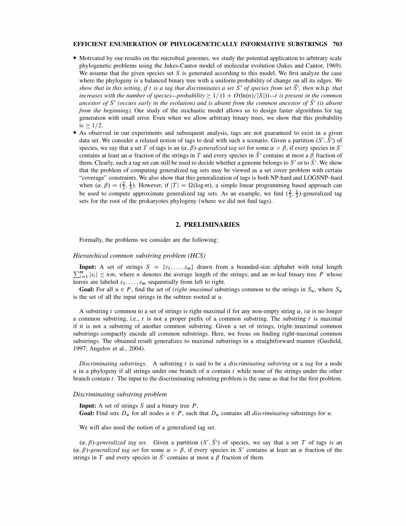
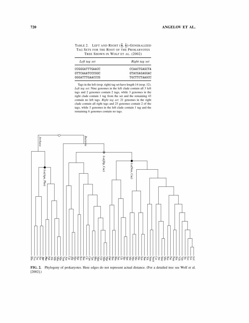
FIG. 2. Phylogeny of prokaryotes. Here edges do not represent actual distance. (For a detailed tree see Wolf et al.

[2002].)


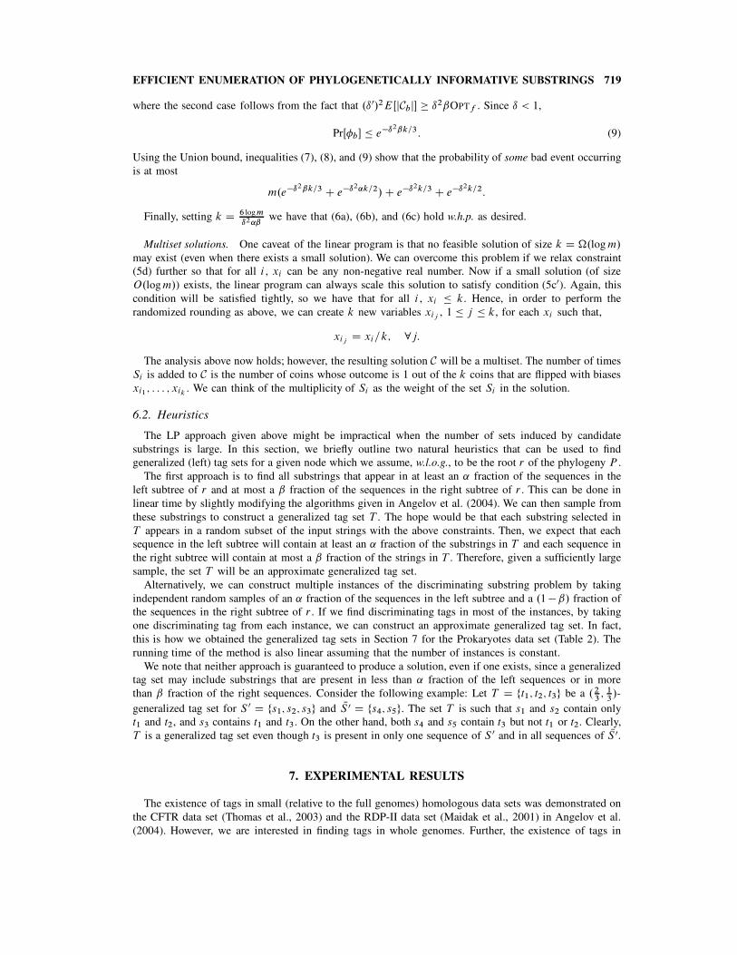
FIG. 3. Length (log-scale) distribution of tags and common substrings for two nodes of the prokaryotes phylogeny

of Wolf et al. (2002). The left (right) panel displays discriminating tags present in the left (right) subtree of thecorresponding node. (a) Tags and common substrings for the lowest common ancestor of Ape (Aeropyrum pernix)

and Pho (Pyrococcus horikoshii). (b) Tags and common substrings for the lowest common ancestor of Nos (Nostoc

sp. PCC 7120) and Cac (Clostridium acetobutylicum).

subsequences of a given set of strings does not necessarily imply the existence of tags in the strings. Herethe existence of tags in data sets containing whole genomes is confirmed on the prokaryotes phylogenyobtained from Wolf et al. (2002).2 The genomes represented in the data set span a broad evolutionarydistance, at the level of one of the three recognized domains of life. But these genomes are also some ofthe smallest (1000-fold smaller than the human genome), allowing less sampling space for tags. Thus, theyrepresent cases on the hard extremes of potential applications. We find left and right tags for all nodes ofthe phylogeny except for the root and the lowest common ancestor of Cac (Clostridium acetobutylicum)and jHp (Helicobacter pylori), where for the latter node only left tags are found. Relaxing the definition ofa tag set as in Section 2, we show two .2

3; 1

3/-generalized tag sets for the root as examples. The prokaryotes

phylogeny consists of 57 genomes where the average genome length is roughly 2:75 Mbp and the totallength is about 157 Mbp. There are 11 sequences in the root’s left subtree (Archaea) and 43 sequencesin its right subtree (Bacteria). For convenience, Figure 2 illustrates the structure of the phylogeny (seeFig. 1 in Wolf et al. [2002]). We implemented the sublinear space algorithm described in Section 4.2 tofind all tags for every node in the tree if they exist. Figure 3a shows both left and right tags for the lowestcommon ancestor of Ape (Aeropyrum pernix) and Pho (Pyrococcus horikoshii), and Figure 3b shows the

2Our experimental results can be found at: www.cis.upenn.edu/!angelov/phylogeny.

722 ANGELOV ET AL.

tags for lowest common ancestor of Nos (Nostoc sp. PCC 7120) and Cac (Clostridium acetobutylicum).As mentioned earlier, we did not find tags for the root of the phylogeny. Hence we generated two .2

3; 1

3/-

generalized tag sets for the root using a heuristic approach described in Section 6.2. Table 2 displaysthose two sets. We also enumerated the common substrings for this phylogeny as shown in Figure 3. Asexpected, longer common substrings are also discriminating tags; i.e., the longer the shared substrings,the more likely they are shared by evolutionary descent (what we call type–I tags in the analysis below).The experimental data suggests that, at least for this range of diversity, our approach will be successful atrecovering informative substrings.

8. DISCUSSION

The data-driven approach to choosing discriminating oligonucleotide sequences appears to be novel. Inthis paper we have described how such sequences can be chosen given a “complete” data set consisting ofa phylogeny where all the input sequences are present at the leaves. In this situation when our algorithmsproduce tags we can use them for high-throughput identification of an unlabeled sequence which is knownto be one of the sequences in the input. Each tag found (at any node in the phylogeny) identifies an exactlyconserved sequence shared by a clade. Such conserved segments can be used as seeds (in a BLAST-likefashion) to identify longer segments with high-similarity multiple alignments. When our algorithm failsto find tags, or even sufficiently long, shared sequences this is also informative. We learn that there is nostrong conservation of segments within the clade. A natural extension of the problem considered here isto the situation where our knowledge is less complete. For example, how can one generalize to the casewhen the phylogeny is not fully known? If we attempt to place a new sequence in the phylogeny usingthe tags to guide us, how good is the placement as a function of the position of the new sequence in thephylogeny vis a vis the sequences from which the tag set was built? These are some of the directions thatwe plan to explore.

ACKNOWLEDGMENTS

We would like to thank Sheng Guo for his help with the simulation experiments and the anonymousreferees for valuable comments and suggestions. This work was supported in part by NIGMS (grant1P20GM69121).

REFERENCES

Amann, R., and Ludwig, W. 2000. Ribosomal RNA-targeted nucleic acid probes for studies in microbial ecology.FEMS Microbiol. Rev. 24, 555–565.

Angelov, S., Harb, B., Kannan, S., et al. 2004. Genome identification and classification by short oligo arrays. Lect.

Notes Comput. Sci. 3240, 400–411.Angelov, S., Harb, B., Kannan, S., et al. 2006. Efficient enumeration of phylogenetically informative substrings. Lect.

Notes Comput. Sci. 3909, 248–264.

Bejerano, G., Pheasant, M., Makunin, I., et al. 2004. Ultraconserved elements in the human genome. Science 304,1321–1325.

Bejerano, G., Siepel, A., Kent, W., et al. 2005. Computational screening of conserved genomic DNA in search of

functional noncoding elements. Nat. Methods 2, 535–545.Brown, M.R., and Tarjan, R.E. 1979. A fast merging algorithm. J. ACM 26, 211–226.

Brown, M.R., and Tarjan, R.E. 1980. Design and analysis of data structures for representing sorted lists. SIAM J.

Comput. 9, 594–614.Chang, W.I., and Lawler, E.L. 1994. Sublinear approximate string matching and biological applications. Algorithmica

12, 327–344.

Gusfield, D. 1997. Algorithms on Strings, Trees, and Sequences. Cambridge University Press, New York.Harel, D., and Tarjan, R.E. 1984. Fast algorithms for finding nearest common ancestors. SIAM J. Comput. 13, 338–355.

Hui, L. 1992. Color set size problem with applications to string matching. Lect. Notes Comput. Sci. 644, 227–240.


Jukes, T.H., and Cantor, C. 1969. Mammalian Protein Metabolism. Academic Press, New York.

Maidak, B.L., Cole, J.R., Lilburn, T.G., et al. 2001. The RDP-II (ribosomal database project). Nucleic Acids Res. 29,173–174.

Matveeva, O.V., Shabalina, S.A., Nemtsov, V.A., et al. 2003. Thermodynamic calculations and statistical correlations

for oligo-probes design. Nucleic Acids Res. 31, 4211–4217.McCreight, E.M. 1976. A space-economical suffix tree construction algorithm. J. ACM 23, 262–272.

Megiddo, N., and Vishkin, U. 1988. On finding a minimum dominating set in a tournament (note). Theoret. Comput.

Sci. 61, 307–316.Papadimitriou, C.H., and Yannakakis, M. 1996. On limited nondeterminism and the complexity of the V-C dimension.

J. Comput. Syst. Sci. 53, 161–170.

Pugh, W. 1990. A skip list cookbook [Technical Report CS-TR-2286.1]. University of Maryland Institute for AdvancedComputer Studies.

Schieber, B., and Vishkin, U. 1988. On finding lowest common ancestors: simplifications and parallelization. SIAM J.

Comput. 17, 1253–1262.Siepel, A., Bejerano, G., Pedersen, J., et al. 2005. Evolutionarily conserved elements in vertebrate, insect, worm, and

yeast genomes. Genome Res. 15, 1034–1050.

Stanley, R.P. 1999. Enumerative Combinatorics. Volume 2. Cambridge University Press, Cambridge, UK.Thomas, J., Touchman, J., Blakesley, R., et al. 2003. Comparative analyses of multi-species sequences from targeted

genomic regions. Nature 424, 788–793.

Ukkonen, E. 1995. On-line construction of suffix trees. Algorithmica 14, 249–260.Weiner, P. 1973. Linear pattern matching algorithms. Proc. 14th IEEE Symp. Switching Automata Theory, 1–11.

Wolf, Y.I., Rogozin, I.B., Grishin, N.V., et al. 2002. Genome trees and the tree of life. Trends Genet. 18, 472–479.

Address reprint requests to:Dr. Stanislav Angelov

Department of Computer and Information Science

University of Pennsylvania

3330 Walnut St.

Philadelphia, PA 19104

E-mail: [email protected]

efï¬cient enumeration of phylogenetically informative substrings

Documents