1

Efficient Serial and Parallel Algorithms for

Querying Large Scale Multidimensional Time

Series Data

Joseph JaJa,Fellow, IEEE,Jusub Kim, and Qin Wang,

Authors are with the Institute for Advanced Computer Studies, Department of Electrical and Computer Engineering, University

of Maryland, College Park, MD 20742, E-mail:{joseph, jusub, qinwang}@umiacs.umd.edu

July 6, 2004 DRAFT

2

Abstract

We consider the problem of querying large scale multidimensional time series data to discover

events of interest, test and validate hypotheses, or to associate temporal patterns with specific events.

Multidimensional time series data is growing at an extremely fast rate due to a number of trends including

a recent strong interest in collecting and analyzing time series of business, scientific, demographic, and

simulation data. The ability to explore such collections interactively, even at a coarse level, will be critical

to the process of extracting some of the information and knowledge embedded in such collections. We

develop indexing techniques and search algorithms to efficiently handle temporal range value querying

of multidimensional time series data. Our indexing uses linear space data structures that enable the

handling of queries very efficiently, invoking in the worst case a logarithmic number of queries to single

time steps. We also show that our algorithm is ideally suited for parallel implementation on clusters of

processors achieving a linear speedup in the number of available processors. A particularly simple data

structure with provably good bounds is also presented for the case when the number of multidimensional

objects is relatively small. These techniques improve significantly over previous techniques for either

the serial or the parallel case, and are evaluated by extensive experimental results that confirm their

superior performance. In particular, we achieve query times in the order of hundreds of milliseconds on

a (relatively outdated) cluster of16 processors for 140GB of data consisting of160, 000 distinct time

series of16-dimensional points, each time series being of length10, 000.

Index Terms

Indexing methods, range query processing, multidimensional time series, spatial query processing,

interactive data exploration and discovery.

I. I NTRODUCTION

While considerable work has been performed on indexing multidimensional data (see for

example [1]), relatively little efforts have been made for developing techniques that specifically

deal with time series of multidimensional data. However, such type of data is abundantly

available, and is currently being generated at an unprecedent rate in a wide variety of applications

that include environmental monitoring, scientific simulations, medical and financial databases,

and demographic studies. For example, the remotely sensed data generated by the NASA satellites

alone is expected to exceed several terabytes per day in the next couple of years. This type of

spatio-temporal data constitutes large scale multidimensional time series data that are currently

very hard to manipulate or analyze. Another example involves the tens of thousands of weather

July 6, 2004 DRAFT

3

stations around the world which provide hourly or daily surface data such as precipitation,

temperature, winds, pressure, and snowfall. Such data can be used to model and predict short-

term and long-term weather patterns or correlate spatio-temporal patterns with phenomena such

as storms, hurricanes, or tornados. Similarly, in the stock market, each stock can be characterized

by its daily opening price, closing price, and trading volume, and hence the collection of long

time series of such data for various stocks can be used to understand short and long term financial

trends.

Our general framework consists of a collection ofN time series such that each time series

describes the evolution of an object (point) in multidimensional space as a function of time. A

possible approach for exploring such data can be based on determining which objects behave

in a certain way over some time window. Such exploration can be used for example to test

a hypothesis relating patterns to specific events that happened during that time window or

classifying objects based on their behavior within that time window. Since quite often, we will

be experimenting with many variations of a pattern to determine appropriate correlations to an

event of interest, or experimenting with many variations of the parameters of a certain hypothesis

to test its validity, it is critical that each exploration be achieved interactively, preferably on the

available large scale multidimensional data without sampling or summarization. This approach

should be viewed as complementary to the standard data exploration approach, which is based

on extracting statistical and summary information about subsets of the data. We focus in this

paper on techniques that minimize the overall number of I/O accesses and that are suited for

sequential implementation as well as parallel implementation on clusters of processors.

Current multidimensional access techniques handle two types of multidimensional objects,

points and extended objects such as lines, polygons, or polyhedra. In this paper we restrict

ourselves to multidimensional point data and address the temporal extensions of the orthogonal

range value queries, which constitute the most fundamental type of queries for multidimensional

data. This type of queries is introduced next.1

Given N objects, each specified by a set ofd attributes, letOi(l) indicate thelth attribute

value of objecti.

1In the remainder of this paper, an object refers to a multidimensional point.

July 6, 2004 DRAFT

4

Query 1-1. (Orthogonal Range Value Query in Multidimensional Space)Given d value

ranges[al, bl], 1 ≤ l ≤ d, determine the set of objects that fall within the query rectangle defined

by these ranges.

RangeQ={Oi| al ≤ Oi(l) ≤ bl, for ∀l, 1 ≤ l ≤ d}.For the case of multidimensional time-series data, we are primarily interested in addressing the

multidimensional data trends along the time axis. By incorporating the time-interval component,

we can extend the above types of queries into two special cases and a more general case.

Given m time snapshots ofN d-dimensional objects at time instancest1, t2, · · · , tm, let Oji (l)

denote thelth attribute value of objecti at time tj.

Query 2-1. (Conjunctive Temporal Range Value Query)Given d value ranges[al, bl], 1 ≤l ≤ d, and a time interval[ts, te], determine the set of objects that fall within the query range

values during every time instance that appears in the interval[ts, te].

TRangeQ1={Oi| al ≤ Oji (l) ≤ bl, for ∀l, 1 ≤ l ≤ d at ∀j time stamps,ts ≤ tj ≤ te}.

Query 2-2. (Disjunctive Temporal Range Value Query)Givend value ranges[al, bl], 1 ≤ l ≤d, and a time interval[ts, te], determine the set of objects that fall within the query range values

at some time instance within[ts, te].

TRangeQ2={Oi| al ≤ Oji (l) ≤ bl, for ∀l, 1 ≤ l ≤ d for somej, ts ≤ tj ≤ te}.

Query 2-3. (General Temporal Range Value Query)Givend value ranges[al, bl], 1 ≤ l ≤ d,

a time interval[ts, te], and a fraction0 < p ≤ 1, determine the set of objects, each of which

falls within the query range values in at least a certain fractionp of time steps during the query

time interval.

TRangeQ3={Oi| al ≤ Oji (l) ≤ bl, for ∀l, 1 ≤ l ≤ d for at least a fractionp, (0 < p ≤ 1), of

time steps during the time interval[ts, te]}.In this paper, we focus on Query 2-1 and introduce very efficient strategies to handle such

queries. The performance of our techniques is confirmed by extensive simulation results on

widely different types of synthetic data. Both the sequential and parallel performances are shown

to be substantially superior to what can be achieved with standard techniques.

July 6, 2004 DRAFT

5

A. Possible Approaches Based on Standard Techniques

A special case of our problem is the well-studied orthogonal range search problem. There

are two straightforward ways to extend related multidimensional access technique to handle the

above queries. The first consists of viewing the multidimensional time series data in(d + 1)

dimensions, and use existing techniques to handle the temporal range queries. This implies that

object i at time tj is represented by the coordinates(Oji (1), Oj

i (2), · · · , Oji (d), tj) in (d + 1)

dimensional space, i.e., the evolution of an object alongm time instances is represented bym

points in(d+1)-dimensional space. Such an approach can also be couched within the framework

explored forgeneralized intersection searching[2], which translates into coloring each point in

(d + 1)-dimensional space with its object id. Hence them points describing the evolution of

object i are colored with colori. As a result, the temporal range queries are transformed into

determining the distinct colors that appear at a certain frequency within the query rectangle. For

example, Query 2-2 amounts to determining the number of distinct colors (and hence object ids)

of the points that fall within the(d + 1)-dimensional query rectangle. The best known internal

memory algorithms for special cases of this problem appear in [3] but no external memory

algorithms are known to the authors best knowledge.

There are two main disadvantages with such an approach. The first is the fact that, for any

time window of sizew, the search algorithm, based on any technique to solve the orthogonal

range value problem, will identify some subset of the correspondingw points of each object,

which fall within the query range values. Hence, the number of candidate points explored can

be arbitrarily larger than the output size (consisting of the indices of the objects that satisfy the

query), which is undesirable especially for large time windows. The second disadvantage is the

fact that the resulting data structure, say an R-tree[4] or any of its variants [5], [6], [7], [8],

cannot be easily handled on a cluster of processors and corresponding parallel search algorithms

tend to be complex and not linearly scalable. Our simulation results will illustrate the substantial

inferior performance of such an approach relative to our new approach, even for the case of a

single processor.

The second straightforward approach would be to build a multidimensional indexing data

structure for thed-dimensional points at each time instance, and then sequentially search each

of the data structures for each time instance of the query interval. This approach, while easy to

July 6, 2004 DRAFT

6

implement, can be quite inefficient and will generate, as we proceed along the time axis, many

possible candidates most of which will be ruled out by the end of the process. Moreover, while

this strategy leads to a fast parallel implementation by analyzing all the time steps in parallel, the

number of processors required will grow linearly with the length of the query interval, as opposed

to our strategy that will linearly scale with any constant number of processors, independent of

the length of the time interval, and will report each proper object only once.

A more involved approach can be based on more sophisticated data structures such as MR-

tree[8], Historical R-tree(HR-tree)[9][10], and RT-tree[8]. These data structures focus on reducing

the redundancy in a series of R-trees built along the time axis by making use of identical branches

in consecutive R-trees. None of these techniques are appropriate for our problem since the only

possible strategy seems to involve proceeding sequentially in time through the different temporal

versions, which amounts in the worst case to at least the same amount of work as that required

by the second straightforward approach.

A related class of problems that have been studied in the literature, especially the database

literature, deals with time series data by appending a timestamp (or a time interval) to each piece

of data separately, thus treating each record, rather than each object, as an individual entity. As

far as we can tell, none of these techniques yield efficient solutions to the problems addressed

here. Examples of such techniques include the Multiversion B-tree [11], Multiversion Access

Methods [12], and the Overlapping B+-trees [13].

We should note that special cases of our problem were addressed in [14] in the case of internal

memory algorithms.

B. Computational Model

Before proceeding further, we introduce our computational model, which is (more or less) the

standard I/O model used in the literature [15]. This model is defined by the following parameters:

n, the size of the input;M , the size of the internal memory; andB, the size of a disk block. An

I/O operation is defined as the transfer of one block of contiguously stored data between disk

and internal memory. Hence, scanningn contiguously stored items takesO(n/B) I/O operations.

In the parallel domain, we assume the presence ofp processors, each with its own disk drive,

such that thep processors are connected through a commodity interconnection network. Each

July 6, 2004 DRAFT

7

I/O operation by a processor involves the transfer of a block ofB consecutive words. Forp = 1,

we obtain the standard I/O model.

II. OVERALL STRATEGY FORTEMPORAL RANGE QUERYING

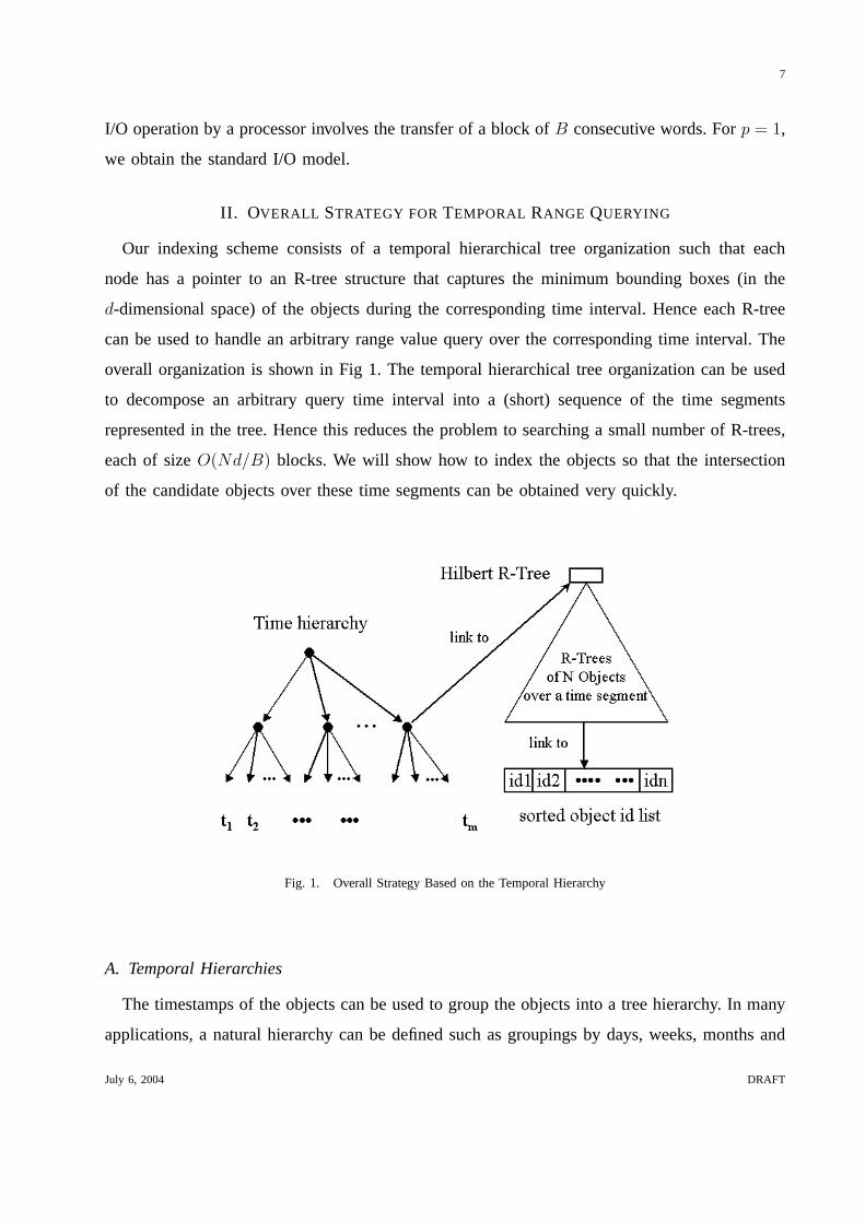
Our indexing scheme consists of a temporal hierarchical tree organization such that each

node has a pointer to an R-tree structure that captures the minimum bounding boxes (in the

d-dimensional space) of the objects during the corresponding time interval. Hence each R-tree

can be used to handle an arbitrary range value query over the corresponding time interval. The

overall organization is shown in Fig 1. The temporal hierarchical tree organization can be used

to decompose an arbitrary query time interval into a (short) sequence of the time segments

represented in the tree. Hence this reduces the problem to searching a small number of R-trees,

each of sizeO(Nd/B) blocks. We will show how to index the objects so that the intersection

of the candidate objects over these time segments can be obtained very quickly.

Fig. 1. Overall Strategy Based on the Temporal Hierarchy

A. Temporal Hierarchies

The timestamps of the objects can be used to group the objects into a tree hierarchy. In many

applications, a natural hierarchy can be defined such as groupings by days, weeks, months and

July 6, 2004 DRAFT

8

years. If no such natural hierarchy exists, we can use a balancedk-ary tree for some value ofk

that depends on the application. Once the hierarchy is set, any temporal range can be decomposed

into a series of time segments (days, weeks, months, for instance) represented by the nodes in

the tree hierarchy. Therefore, a temporal range query can be answered by issuing a series of

temporal range queries on the corresponding time segments. For the remainder of the paper, we

take k = 2, in which case one can easily show that the number of nodes in the binary tree

needed to accommodate any time window is logarithmic in the size of the time window. The

qualified objects consist of the intersection or union of the results at the corresponding nodes,

depending on the type of the query. Given any node in the tree hierarchy, the non-temporal data

attributes of the objects can be aggregated over the corresponding time segment into an auxiliary

structure attached to the node corresponding to that time segment. In our case, the minimum

and maximum attribute values for each object over the time segment are computed and stored.

B. Rectangle Containment Query

For a fixed time segment, the attributes of each object lie within the rectangle defined by

the minimum and the maximum values of each attribute over this time segment. The handling

of Query 2-1 comes down to determining the objects whose rectangles are fully contained in

the query rectangle (defined by the range values). Given that we expect the number of objects

to be very large (with the number of attributes ranging typically between 1 and 20), the data

corresponding to each time step is typically too large to fit in main memory. We will represent

the set of rectangles stored at each node of the time hierarchy by an R-tree that makes use of

Hilbert space filling curves. Such R-trees seem to work well in practice even for a moderately

high number of dimensions. We adapt such a strategy to our problem as follows.

Each leaf of the time hierarchy requires an R-tree to represent the correspondingN d-

dimensional points, and hence this can be built using the standard Hilbert R-tree. Each interior

node of the time hierarchy requires an R-tree that represents the correspondingN rectangles in

d dimensions. Such an R-tree can be built by sorting the rectangles according to their Hilbert

indices (properly defined), and proceeding in a sequence of hierarchical groupings as in the

standard way to build a Hilbert R-tree. However we attach additional information at each node

as follows.

We associate with each internal R-tree node a pointer to an ID list corresponding to the objects

July 6, 2004 DRAFT

9

stored in its subtree. We make use of this ID list as follows. Suppose that, during the search,

a minimum bounding rectangle in the R-Tree is found to be fully enclosed within the query

rectangle. This means that all the objects contained inside this minimum bounding rectangle

satisfy the query relative to the time window. Hence we can use the list of IDs to determine

these objects, without having to proceed further down the R-tree as in the standard search process.

In fact, based on the way we constructed the R-tree, we can create an overall list of IDs sorted by

their Hilbert indices, and then represent each Id list at a node by two pointers to the overall list.

All consecutive objects between these two pointers fall within the Minimum Bounding Rectangle

(MBR) of that node. Since the size of object ID list is small, multiple consecutive accesses can

be carried out through buffering in memory, which substantially improves our R-Ttree search

time, almost independent of the number of qualified objects.

C. Query Algorithm

We first focus on the algorithm to handle Query 2-1, assuming a single processor.

We start by determining the minimum number of nodes in the temporal hierarchy required to

handle the query time window. Our time hierarchy is a balanced binary tree stored as a linear

array in internal memory, and hence this step is quite simple and can be carried out very quickly.

At the end of this step, we identifyO(log m) nodes, each with a pointer to an R-tree.

Starting with the node representing the longest time segment in the time query window, we

search the corresponding R-tree that was already augmented by the appropriate sorted ID list.

The IDs of objects satisfying the query are returned. The same search process can be performed

on the remaining nodes.

The output list of IDs is generated incrementally by intersecting the returned ID lists from

the various R-tree searches.

D. Parallel Implementation

We now consider the case when there is a cluster ofp processors available, wherep is naturally

much smaller than the total numberN of objects and each processor has its own disk pool. We

divide the correspondingN time series equally among thep processors, and build a separate

indexing for each set ofNp

objects as before, but with a unified time hierarchy of sizeO(m).

July 6, 2004 DRAFT

10

The handling of a query begins with the quick internal memory step to identify the appropriate

nodes of the temporal hierarchy, followed by searching the appropriate R-trees residing in thep

processors. The final step consists of simply merging the non-overlapping sets of indices returned

by the various processors, which can be done on a single processor. It is clear that all the major

computational steps are performed on thep processors in parallel, each working on an indexing

structure forN/p objects, and hence the parallel implementation is linearly scalable in terms of

the number of objects.

This parallel algorithm is ideally suited for the distributed disk model introduced earlier.

However for the case when we have a centralized disk pool, interconnected with a high speed

network to a cluster of processors, the following parallel algorithm will be more suitable. All

the full-size R-trees are stored in the centralized disk pool and the R-trees corresponding to each

level of the temporal hierarchy are allocated to a processor. The handling of a query is reduced

to O(log m/p) full R-tree searches conducted by each of thep processors in parallel. In this case,

the availability of anO(log m) processors will reduce the complexity of the problem to that of

handling an R-tree corresponding to a single time step. These two approaches are complementary

and can be combined to lead to a very efficient parallel implementation on clusters of SMPs

(Shared Memory Symmetric Multiprocessors), where each SMP has a pool of disks. In this

paper, we focus on the distributed disk model.

E. Time and Space Complexity

The space requirement of our overall data structure is clearly linear in the input size since

we haveO(m) R-trees, each is built onN rectangles ind-dimensional space. Handling a query

on a single processor will require the search through at mostO(log m) R-trees, each of size

O(Nd). For the case when we have a cluster ofp processors, our I/O complexity reduces to at

mostO(log m) R-tree searches, each of sizeO(Ndp

), and as we will see later each such R-tree

search can be completed with a speedup of factorp. Hence the overall query algorithm will be

linearly scalable.

July 6, 2004 DRAFT

11

���������������������������

��� ������ ������ ���

���������������

��� ������ ������ ���

���������������������������

��� ������ ������ ���

���������������

��� ������ ������ �����������

��

���������������������������

������������������������������

������������������������������

������������������������������

���������������������������

������������������������������

������������������������������

������������������������������

�� ��� ���

�������

Fig. 2. The minmaxB+-tree data structure. Each key in an interior node holds the minimum and the maximum values of each

attribute of the corresponding child node.

III. E FFICIENT STRATEGIES FOR ASMALL NUMBER OF OBJECTS

In this section, we consider the case when the number of objects is relatively small and provide

a provably good solution to Query 2-1. Our solution builds the time hierarchy on a B+-tree,

whose interior nodes have been augmented with auxiliary information. Specifically, we use a

k-ary tree on the ordered time stamps such that each leaf contains the data corresponding to all

the objects fork consecutive time stamps, all stored inO(Ndk/B) consecutive blocks. For an

interior node, we store in addition to the key splitters, the minimum and maximum values of

each attribute of each object, over the time interval corresponding to each child of the node. We

call such a structure the minmaxB+-tree, which is illustrated in Fig. 2 for the case of a single

object. It is easy to verify that each node is of sizeO(Ndk/B) blocks, the height of the tree is

O(logkm), and the overall size is linear.

The handling of a Query 2-1 proceeds as follows:

1. Determine the lowest common ancestorQ of the leaves of the minmaxB+-tree corresponding

to the start and end time stamps of the query temporal window[ts, te]. Note that this can be done

in internal memory without any I/O accesses.

July 6, 2004 DRAFT

12

2. Let the ith and jth children of Q be those children that are on the paths fromQ to

ts and te respectively. We begin by determining, for each key betweeni and j, the objects

whose minimum and maximum values fall within the query range values. These objects are now

potential candidates for our query. We proceed to check whether there are some objects that also

satisfy the query bounds ati andj. These can be immediately declared as satisfying the query.

We then proceed with the remaining candidates, fromQ along the paths leading tots and te.

3. At each interior node along the paths tots and te, we refine the list of candidates by

checking whether all the attributes’ minimum and maximum values of the children that have

time stamps greater thants or less thante lie within the query range values. If necessary, we

repeat this step until we reach the leaf nodes.

4. At the two leaf nodes to whichts and te belong, we complete the refinement of the list of

the candidates thereby generating a list of the objects that satisfy the query.

Notice that the I/O complexity is proportional to the height of the tree, and hence is of

O(logk m). Each step will takeO(Ndk/B) I/O steps because each node consists ofO(Ndk/B)

blocks. Clearly this is only efficient for small values ofN .

We will present experimental results comparing this approach to the simple approach of using

the standard B+-tree for a single object (which clearly favors the standard B+-tree approach).

Even for this case, our approach is shown to be significantly superior especially for large query

time windows. We also provide experimental results comparing our minmaxB+-tree approach to

our scheme for the general case that uses R-trees. Note that the minmaxB+-tree has provably

optimal bounds wheneverNdk ≤ cB, for some constantc, and the main practical issue is

to determine the highest value ofc for which the approach of this section is superior. The

experimental results show that this approach will indeed be superior whenever the number of

objects is in the thousands. Otherwise, our general approach is superior.

IV. EXPERIMENTAL RESULTS

Our experimental results make use of synthetic data sets generated by a software package

developed at the University of Maryland. We can specify N, d, m, and one of 4 possible

distributions, to generate the corresponding data set. Given the extensive number of experiments

that we needed to conduct and the substantial amounts of data involved, we used three distinct

platforms for our experiments. For the sequential algorithm of the general case, the processor

July 6, 2004 DRAFT

13

used is a Sun Ultrasparc 359 MHz with 512MB main memory, and each of the disks used

is a 9GB disk, 7200 RPM, with I/O throughput of 20 MB/s. For the case of a small number

of objects, we used a Sun Fire-280R 1.2 GHz with 8G main memory, with 10,000RPM disk

whose advertised peak performance is 40 MB/s I/O throughput. For the parallel case, we used

a Linux cluster of 30 IBM Netfinity nodes, each node has a Pentium-III (650 MHz) processor,

768MB memory, and two 80GB disks with I/O transfer rate around 15MB/s. The nodes are

interconnected through 100Mb/s Fast Ethernet.

We start by presenting our main sequential results for the general case, followed by a brief

description of the experimental results corresponding to the case when we have a small number

of objects. The experimental results obtained for the case of a cluster of processors are discussed

last.

A. Sequential Performance for the General Case

For the general case, we tookN = 10, 000 objects, each with a time series of length

m = 10, 000. The value ofd was set to2, 4, 8, and the distributions used were the Gaussian and

the uniform distributions. Our time hierarchy is a balanced binary tree stored in an integer array

of length 19, 999 . For a given input, the performance is measured in terms of the number of

blocks interchanged between the disk and the internal memory, and in terms of the query time.

Given that the performance will depend on the query time window and the query range values,

we describe our results in two parts, the first focusing on the query performance when the size of

the time window changes, and the second focusing on the query performance when the attribute

range values change. We also compare our results to those obtained by incorporating the time

dimension as an additional dimension using a single Hilbert R-tree, and to the sequential scan

over the time window, where we use a Hilbert R-tree for each time instance. The comparison

shows substantial gains achieved by our scheme over these two schemes, even forp = 1. With

more processors, our scheme will achieve even stronger performance relative to the standard

approaches.

1) Performance as a Function of Time Window Length:We conducted a series of tests based

on queries with fixed spatial range values but increasing time windows from a single time step

to a time window of size1000. The results on the 4-D dataset are shown in Fig. 3 through

July 6, 2004 DRAFT

14

Fig. 3. Number of Page Block Accesses vs. Query Time Window Size

Fig. 5, using Gaussian distributions for the first two dimensions and uniform distributions for

the remaining two. Note that each R-Tree takes 256 pages, each page of size 2K. In each case, we

measure the number of accessed page blocks, query time, and the number of R-trees searched.

For these graphs, the starting time used was5001, but the results of other possible starting times

are very similar.

These results clearly indicate that the number of pages accessed and the number of R-trees

searched follow each a logarithmic pattern as a function of the query time window size. The

relative variations from a logarithmic curve fit are small. Another immediate result is that the

query time follows the same logarithmic pattern.

Fig. 6 and Fig. 7 are the performance results of using a single R-tree with the same series of

queries on the same input. Notice that as the time window size increases, the query rectangle

overlaps with more MBRs in the single R-tree, and hence the search algorithm explores many

more paths in the R-tree. This observation is confirmed by the experimental results, which show

a substantial increase in the number of pages accessed and in the query time as the temporal

window size increases.

2) Performance As a Function of the Query Range Values:We now fix the temporal window

size and change the spatial range values gradually until nearly all the objects are included. The

July 6, 2004 DRAFT

15

Fig. 4. Query Time vs. Query Time Window Size

Fig. 5. Number of Qualified Objects vs. Query Time Window Size

July 6, 2004 DRAFT

16

Fig. 6. Number of Accessed Page Blocks vs. Query Time Window Size When Using a Single R-Tree

Fig. 7. Query Time vs. Query Time Window Size When Using a Single R-Tree

July 6, 2004 DRAFT

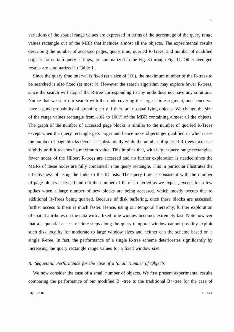
17

variations of the spatial range values are expressed in terms of the percentage of the query range

values rectangle out of the MBR that includes almost all the objects. The experimental results

describing the number of accessed pages, query time, queried R-Trees, and number of qualified

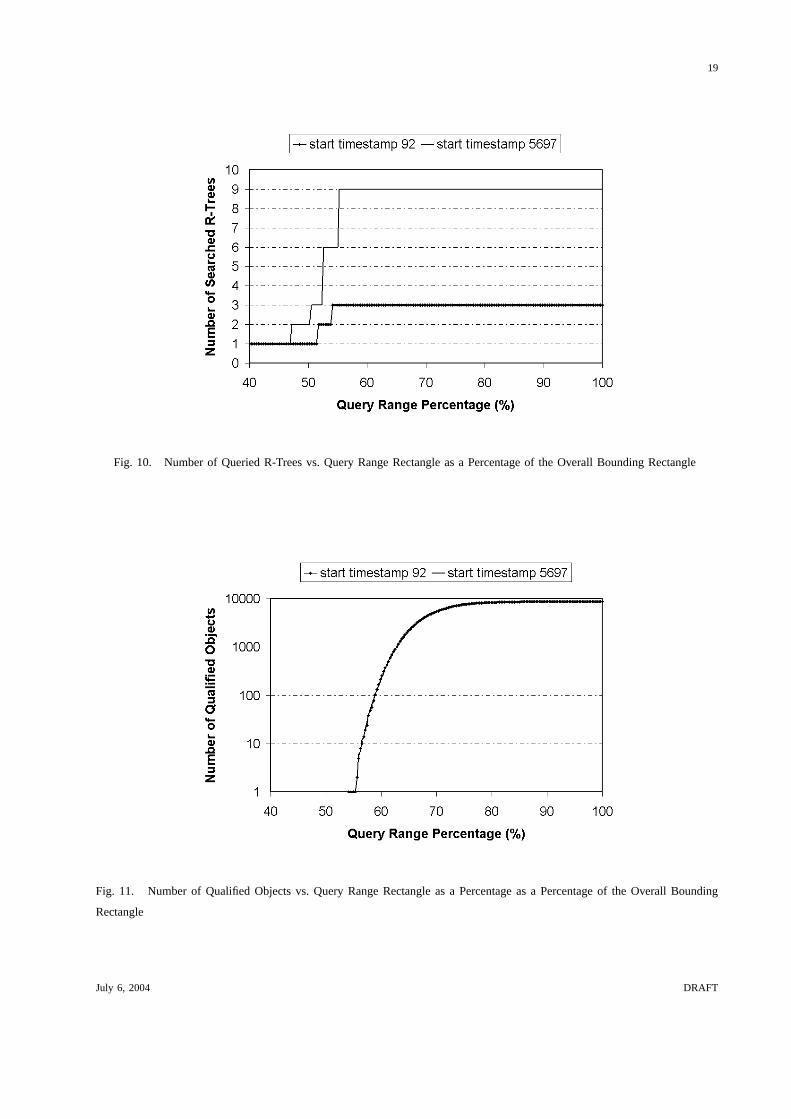
objects, for certain query settings, are summarized in the Fig. 8 through Fig. 11. Other averaged

results are summarized in Table I .

Since the query time interval is fixed (at a size of100), the maximum number of the R-trees to

be searched is also fixed (at most9). However the search algorithm may explore fewer R-trees,

since the search will stop if the R-tree corresponding to any node does not have any solutions.

Notice that we start our search with the node covering the largest time segment, and hence we

have a good probability of stopping early if there are no qualifying objects. We change the size

of the range values rectangle from40% to 100% of the MBR containing almost all the objects.

The graph of the number of accessed page blocks is similar to the number of queried R-Trees

except when the query rectangle gets larger and hence more objects get qualified in which case

the number of page blocks decreases substantially while the number of queried R-trees increases

slightly until it reaches its maximum value. This implies that, with larger query range rectangles,

fewer nodes of the Hilbert R-trees are accessed and no further exploration is needed since the

MBRs of these nodes are fully contained in the query rectangle. This in particular illustrates the

effectiveness of using the links to the ID lists. The query time is consistent with the number

of page blocks accessed and not the number of R-trees queried as we expect, except for a few

spikes when a large number of new blocks are being accessed, which mostly occurs due to

additional R-Trees being queried. Because of disk buffering, once these blocks are accessed,

further access to them is much faster. Hence, using our temporal hierarchy, further exploration

of spatial attributes on the data with a fixed time window becomes extremely fast. Note however

that a sequential access of time steps along the query temporal window cannot possibly exploit

such disk locality for moderate to large window sizes and neither can the scheme based on a

single R-tree. In fact, the performance of a single R-tree scheme deteriorates significantly by

increasing the query rectangle range values for a fixed window size.

B. Sequential Performance for the case of a Small Number of Objects

We now consider the case of a small number of objects. We first present experimental results

comparing the performance of our modified B+-tree to the traditional B+-tree for the case of

July 6, 2004 DRAFT

18

Fig. 8. Number of Accessed Page Blocks vs. Query Range Values Rectangle as a Percentage of the Overall Bounding Rectangle

Fig. 9. Query Time vs. Query Range Rectangle as a Percentage of the Overall Bounding Rectangle

July 6, 2004 DRAFT

19

Fig. 10. Number of Queried R-Trees vs. Query Range Rectangle as a Percentage of the Overall Bounding Rectangle

Fig. 11. Number of Qualified Objects vs. Query Range Rectangle as a Percentage as a Percentage of the Overall Bounding

Rectangle

July 6, 2004 DRAFT

20

Dimension 4 8

Interval length 100 1000 100 1000

Ave. Query Time (ms) 160 275 200 350

Ave. Queried R-Trees 6 10 6 10

TABLE I

AVERAGE QUERY TIME AND NUMBER OF QUERIED R-TREES AT VARIOUS QUERY INTERVAL SITUATIONS UNDER RANGE

CHANGING

a single object, which clearly favors the latter. After that, we will present comparison results

between our R-tree based approach and the B+-tree based approach.

For the first experiment, our test data consists of 200,000 time stamps and four attributes at

each time stamp, where the values of each attribute are generated using a gaussian distribution.

A sample of the data generated is shown in Fig. 12. Both the original B+-tree and the new

minmaxB+ tree were built on the same data set. The block size was set to 8 KB and both

versions of the B+tree were of height3.

Fig. 12. A sample synthetic time series data used in the experiment.

The primary benefit of our proposed data structure is that query response time does not depend

on the query time window size. Fig. 13 shows the relationship between the query response time

and query time window size. As seen in the figure, the query time of the traditional B+-tree

increases as the query time window increases. The same figure shows that the query response

time of our proposed minmaxB+-tree is around 20 msec regardless of the size of the query time

window. Note that the average number of blocks accessed using the minmaxB+-tree is between

just 1 and 3 regardless of the query time window size, while the number of blocks accessed

July 6, 2004 DRAFT

21

increases from 3 to 498 as the query time window increases when using the original B+tree.

Fig. 13. Response time versus query time window size, with query range fixed at 80%. Both the original B+tree and the

minmaxB+tree are built on 200,000 time stamps and have three levels.

We should note that the size of our data structure and the construction time are almost the

same as those for the B+ tree. This is due to the fact that we only added some extra information

to the nonleaf nodes which are typically a small part of the total indexing structure. For example,

in this experiment, our indexing structure was larger by 38KB compared to the original B+-tree

that was of size 4MB.

As mentioned earlier, a practical concern is to determine the case for which the approach

is superior to the general approach. Fig. 14 compares the performance of the two approaches

for N = 5, 000, N = 10, 000, d = 8, 16, andm = 10, 000. Fig. 14 demonstrates the superior

performance of the minmaxB+-tree approach whenever the number of objects is in the thousands,

especially when the number of dimensions is high, regardless of the value ofm (since both

approaches use a time hierarchy over them time steps).

C. Performance on a Cluster of Processors

We use two sets of test data, each of which consisting of160, 000 objects over10, 000 time

steps such that the data values are generated by alternating between the Gaussian and Uniform

distributions along the different dimensions. The objects in the first test data set are8-dimensional

July 6, 2004 DRAFT

22

Fig. 14. Comparison between the two approaches in response time: Each series is represented by

[numberofobjects][dimension][blocksize] and all series have 10,000 time stamps.

objects, while those of the second data set are16-dimensional. Hence the sizes of the two data

sets are respectively70GB and140GB.

We ran our experiments using temporal window sizes1, 62, and 1022. As described earlier,

our parallel strategy consists of partitioning160, 000 objects equally among the numberp of

available processors, where in our casep = 1, 2, 4, 16. A unified temporal hierarchy on10, 000

time steps was created, and each processor built the R-trees corresponding to its set of objects.

The query is broadcast to all the processors, followed by each processor conducting the search

on its local R-trees. The final result is obtained by merging the separate lists of indices returned

on a single processor. We measured the average execution time, for each window size, number

of processors, and each data set. The results are summarized in Figures 15, and 16 for the

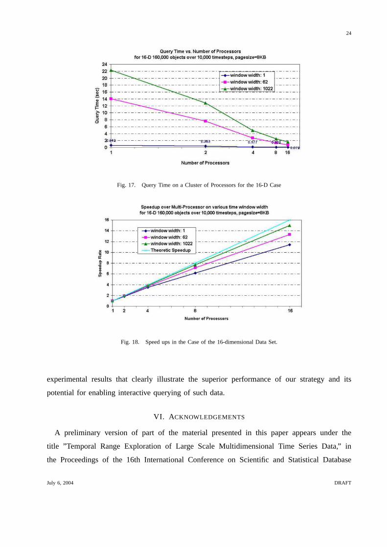
8-dimensional data set, and in Figures 17, and 18 for the16-dimensional data set.

These experimental results illustrate the linear speedups achieved by our algorithm, and the

ability to achieve query execution times in the order of hundreds of milliseconds for140GB of

16-dimensional data on a relatively outdated cluster of16 processors. Note that the superlinear

speedup that occurs when we move from2 processors to4 can be explained by the non-linear

behavior of R-tree searches, especially in our case where a search can terminate very quickly

July 6, 2004 DRAFT

23

Fig. 15. Query Time on a Cluster of Processors

Fig. 16. Speed ups in the Case of the 8-dimensional Data Set.

near the root of the R-tree.

V. CONCLUSION

We considered in this paper the problem of temporal range value querying of large scale

multidimensional time series data. We developed a strategy that reduces the overall problem to

handlingO(log m) versions of single time steps, which also can be mapped onto a cluster of

processors with very little communication overhead. We reported on some of our extensive

July 6, 2004 DRAFT

24

Fig. 17. Query Time on a Cluster of Processors for the 16-D Case

Fig. 18. Speed ups in the Case of the 16-dimensional Data Set.

experimental results that clearly illustrate the superior performance of our strategy and its

potential for enabling interactive querying of such data.

VI. A CKNOWLEDGEMENTS

A preliminary version of part of the material presented in this paper appears under the

title ”Temporal Range Exploration of Large Scale Multidimensional Time Series Data,” in

the Proceedings of the 16th International Conference on Scientific and Statistical Database

July 6, 2004 DRAFT

25

Management, Santorini, Greece, June 2004. This work was supported by the National Science

Foundation through the National Partnership for Advanced Computational Infrastructure under

the PACI Program, and NASA under the ESIP Program NCC5300.

REFERENCES

[1] V. Gaede and O. G̈unther, “Multidimensional access methods,”ACM Computing Surveys, vol. 30, no. 2, pp. 170–231,

1998. [Online]. Available: citeseer.nj.nec.com/gaede97multidimensional.html

[2] R. Janardan and M. Lopez, “Generalized intersection searching problems,”International Journal of Computational

Geometry & Applications, vol. 3, no. 1, pp. 39–69, 1993.

[3] Q. Shi and J. JaJa, “Optimal and near-optimal algorithms for generalized intersection reporting on pointer machines,” in

Technical Report CS-TR-4542, Institute for Advanced Computer Studies, University of Maryland, 2003.

[4] A. Guttman, “R-trees:a dynamic index structure for spatial searching,”ACMSIGMOD, pp. 47–57, 1984.

[5] T. K. Sellis, N. Roussopoulos, and C. Faloutsos, “The r+-tree: A dynamic index for multi-dimensional objects,” inThe

VLDB Journal, 1987, pp. 507–518. [Online]. Available: citeseer.nj.nec.com/sellis87rtree.html

[6] I. Kamel and C. Faloutsos, “Hilbert R-tree: An Improved R-tree using Fractals,” inProceedings of the Twentieth

International Conference on Very Large Databases, Santiago, Chile, 1994, pp. 500–509. [Online]. Available:

citeseer.nj.nec.com/kamel94hilbert.html

[7] N. Beckmann, H.-P. Kriegel, R. Schneider, and B. Seeger, “The r*-tree: an efficient and robust access method for points

and rectangles,” inProceedings of the 1990 ACM SIGMOD international conference on Management of data. ACM

Press, 1990, pp. 322–331.

[8] X. X. J. Han and W. Lu, “RT-tree: An Improved R-tree Index Structure for Spatiotemporal Databases,” inProceedings of

the 4th International Symposium on Spatial Data Handling, 1990, pp. 1040–1049.

[9] M. Nascimento and J. Silva, “Towards Historical Rtrees,” inProceedings of ACM Symposium on Applied Computing

(ACM-SAC), 1998, pp. 235–240.

[10] Y. Tao and D. Papadias, “Efficient Historical R-trees,” inProceedings of the 13th IEEE Conference on

Scientific and Statistical Database Management(SSDBM), Fairfax Virginia, 2001, pp. 223 –232. [Online]. Available:

http://www.cs.ust.hk/faculty/dimitris/PAPERS/ssdbm01.pdf

[11] S. Lanka and E. Mays, “Fully persistent b+-trees,” inProceedings of the ACM SIGMOD International Conference on

Management Data, 1991, pp. 426–435.

[12] P. Varman and R. M. Verma, “An efficient multiversion access structure,”IEEE Transactions on Knowledge and Data

Engineering, vol. 9.

[13] Y. Manolopoulos and G. Kapetanakis, “Overlapping b+-trees for temporal data,” inProceedings of the 5th Jerusalem

Conference on Information Technology, 1990, pp. 491–498.

[14] Q. Shi and J. JaJa, “Fast Algorithms for a Class of Temporal Range Queries,” inProceedings of Workshop on Algorithms

and Data Structures, 2003, pp. 91–102.

[15] J. S. Vitter, “External memory algorithms and data structures: dealing with massive data,”ACM Computing Surveys,

vol. 33, no. 2, pp. 209–271, 2001. [Online]. Available: citeseer.nj.nec.com/vitter00external.html

July 6, 2004 DRAFT