efficient similarity join and search on multi-attribute...
TRANSCRIPT

Efficient Similarity Join and Search on Multi-Attribute Data
Guoliang Li† Jian He† Dong Deng† Jian Li‡†Department of Computer Science, Tsinghua University, Beijing, China
‡Institute for Interdisciplinary Information Sciences, Tsinghua University, Beijing, China{liguoliang, lijian83}@tsinghua.edu.cn; {hejian13, dd11}@mails.tsinghua.edu.cn
ABSTRACTIn this paper we study similarity join and search on multi-attribute data. Traditional methods on single-attribute datahave pruning power only on single attributes and cannote�ciently support multi-attribute data. To address thisproblem, we propose a prefix tree index which has holis-tic pruning ability on multiple attributes. We propose acost model to quantify the prefix tree which can guide theprefix tree construction. Based on the prefix tree, we devisea filter-verification framework to support similarity searchand join on multi-attribute data. The filter step prunes alarge number of dissimilar results and identifies some candi-dates using the prefix tree and the verification step verifiesthe candidates to generate the final answer. For similar-ity join, we prove that constructing an optimal prefix treeis NP-complete and develop a greedy algorithm to achievehigh performance. For similarity search, since one prefixtree cannot support all possible search queries, we extendthe cost model to support similarity search and devise abudget-based algorithm to construct multiple high-qualityprefix trees. We also devise a hybrid verification algorithmto improve the verification step. Experimental results showour method significantly outperforms baseline approaches.
Categories and Subject DescriptorsH.2 [Database Management]: Database applications;H.3.3 [Information Search and Retrieval]: Search process
KeywordsSimilarity Search; Similarity Join; Multi-Attribute Data
1. INTRODUCTIONReal-world data is rather dirty due to typographical errors
and di↵erent representations of the same entity [11]. Tra-ditional exact-matching join and search operations cannottolerate the dirty data and thus similarity join and searchare recently proposed to tolerate the dirty data. Given twomulti-attribute tables (e.g., products and movies), similar-ity join finds all similar pairs from the two tables, where thesimilarity can be quantified by similarity functions, e.g., edit
Permission to make digital or hard copies of all or part of this work for personal or
classroom use is granted without fee provided that copies are not made or distributed
for profit or commercial advantage and that copies bear this notice and the full cita-
tion on the first page. Copyrights for components of this work owned by others than
ACM must be honored. Abstracting with credit is permitted. To copy otherwise, or re-
publish, to post on servers or to redistribute to lists, requires prior specific permission
and/or a fee. Request permissions from [email protected].
SIGMOD’15, May 31–June 4, 2015, Melbourne, Victoria, Australia.
Copyright
c� 2015 ACM 978-1-4503-2758-9/15/05 ...$15.00.
http://dx.doi.org/10.1145/2723372.2723733.
distance and Jaccard. Given a table with multiple attributesand a query, similarity search finds the records from the ta-ble that are similar to the query. Similarity join and searchare two important operations in data cleaning and integra-tion and have many real-world applications, e.g., duplicatedetection, data fusion, and spell checking [11]. For exam-ple, in the event of plane crash like Malaysia airlines flightMH17, there are many data sources about passengers onMH17, e.g., tables from Malaysia airlines, departure coun-try, destination county, and passengers’ countries. We re-quire to integrate them to generate high-quality data. Asanother example, a user wants to search movies directedby “James Cameron” and acted by “Arnold Schwarzenegger”from a movie database with actors, directors, and movienames. However the user does not know the exact spellingof “Arnold Schwarzenegger” and inputs a query with ty-pos. Obviously exact-matching search cannot find any re-sults while similarity search can alleviate this problem andhelp the user to find the relevant answers.
Existing algorithms on string similarity join [20,26,28,29]and search [9,14,15,22,30] have pruning power only on singleattributes. For similarity join and search with constraints onmultiple attributes, they have to first use a single attributeto identify candidates and then check whether the candi-dates satisfy the constraints on other attributes. Obviouslythese algorithms are rather expensive because they have nopruning power on other attributes and generate many in-termediate results. It calls for e↵ective methods to supportholistic similarity join and search on multi-attribute data.
To address this problem, we propose a prefix tree indexwhich has holistic pruning power on multiple attributes.Based on the prefix tree, we devise a filter-verification frame-work. The filter step prunes a large number of dissimilarresults and identifies some candidates using the prefix treeand the verification step verifies the candidates to gener-ate the final answer. For similarity join, we propose a costmodel to quantify the prefix tree. We prove that construct-ing an optimal prefix tree is NP-complete and we developa greedy algorithm to achieve high performance. Di↵erentfrom similarity join, one prefix tree cannot support all pos-sible search queries with di↵erent similarity functions andthresholds. To address this issue, we extend the cost modelto support similarity search. We develop a budge-based al-gorithm to build high-quality prefix trees to achieve highsearch performance. Since the similarity join and searchqueries contain multiple attributes, the verification order onattributes has a significant e↵ect on the verification perfor-mance. In addition, many filtering algorithms can be used
to verify the candidates which also have a great e↵ect onthe performance. To this end, we devise a hybrid algorithmto improve the verification performance. To summarize, wemake the following contributions. (1) We propose a prefixtree index which has holistic pruning power on multiple at-tributes and can be utilized to support both similarity joinand search queries. (2) For similarity join, we develop a costmodel to quantify the prefix tree. We prove that construct-ing an optimal prefix tree is NP-complete and we develop agreedy algorithm to construct a high-quality prefix tree (seeSection 3). (3) For similarity search, we devise a budget-based method to construct multiple high-quality prefix treesto support similarity search queries (see Section 4). (4) Wepropose a hybrid verification algorithm to improve the ver-ification performance (see Section 5). (5) Experimental re-sults on real-world datasets show our method significantlyoutperforms baseline approaches (see Section 6).
2. PRELIMINARIESWe first formally define the problem in Section 2.1 and
then briefly introduce a well-known technique – prefix filterin Section 2.2. Lastly, we review related works in Section 2.3.
2.1 Problem DefinitionConsider two multi-attribute tables R and S. Table R has
x attributes R1
,R2
, · · · ,Rx and m rows r1
, r
2
, · · · , rm
. Ta-ble S has y attributes S1
,S2
, · · · ,Sy and n rows s1
, s
2
, · · · , sn
.Let r
p
= [r1p
, r
2
p
, · · · , rxp
] where r
i
p
denotes the value of rp
onattribute Ri, and s
q
= [s1q
, s
2
q
, · · · , syq
] where s
j
q
denotes thevalue of s
q
on attribute Sj .An atomic similarity join operation Ri ⇠ Sj returns all
similar pairs {(rp
2 R, s
q
2 S)} such that rip
⇠ s
j
q
, where ⇠is a similarity operator which will be defined later.A complex similarity join operation is composed by more
than one atomic similarity join operation, e.g., � = Ri1 ⇠Sj1 ^ Ri2 ⇠ Sj2 ^ · · · ^ Rik ⇠ Sjk , which finds all similarpairs {(r
p
2R, s
q
2S)} such that ri1p
⇠ s
j1q
^ r
i2p
⇠ s
j2q
^ · · · ^r
ikp
⇠ s
jkq
where 8t2[1, k], i
t
2[1, x] and j
t
2[1, y]. We call�
t
=Rit⇠Sjt a predicate or attribute if the context is clear.We utilize similarity measures to define the similarity op-
erator ⇠, which can be broadly classified into two categories,character-based similarity and token-based similarity.Character-based Similarity. It defines the similarity be-tween two strings based on character transformations. Thewell-known character-based similarity is edit distance. Con-sider two string values ri
p
and s
j
q
. The edit distance ED(rip
, s
j
q
)is the minimum number of single-character edit operations(including insertion, deletion and substitution) needed totransform r
i
p
to s
j
q
. The edit similarity extends edit distanceby taking into account the string length, which is defined
as ES(rip
, s
j
q
) = 1 � ED(r
ip,s
jq)
max(|rip|,|sjq |)
, where |rip
| is the length of
r
i
p
. Two strings r
i
p
and s
j
q
are similar with respect to editsimilarity if their similarity exceeds a given threshold ⌧ , i.e.,
r
i
p
ES,⌧⇠ s
j
q
i↵. ES(rip
, s
j
q
) � ⌧.
For example, given the Name attribute of table R in Fig-ure 1, r1
1
= ‘Jeffery Ullman’, r14
=‘Jeffer Ullman’. We haveED(r1
1
, r
1
4
) = 1 and ES(r11
, r
1
4
) = 1� 1
14
= 13
14
.Token-based Similarity. It first splits each string into aset of tokens by white spaces and then utilizes the set-basedsimilarity functions to quantify the similarity. The well-
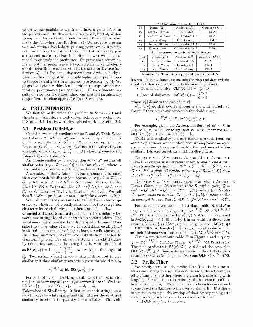
R : Customer records of BOA
Id Name (R1) Address (R2) Country (R3)
r1 Je↵ery Ullman EE UCLA USA
r2 Jennifer Widom CS Stanford CA USA
r3 Jerry Wang CS Berkeley ENG
r4 Je↵er Ullman CS Stanford CA USA
r5 Don Antenio CS Stanford CA USA
S : Customer records of Wells Fargo
Id Name (S1) Address (S2) Country (S3)
s1 Je↵ery Ullman Stanford CA USA
s2 Herry Wang Berkeley CA ENG
s3 Don Ertenio CS Berkeley ENG
Figure 1: Two example tables: R and S.known similarity functions include Overlap and Jaccard, de-fined as below (see Appendix B for more functions).
• Overlap similarity: OLP(rip
, s
j
q
) = |rip
\ s
j
q
|• Jaccard similarity: JAC(ri
p
, s
j
q
) =|rip\s
jq |
|rip[s
jq |
where |rip
| denotes the size of set rip
.r
i
p
and s
j
q
are similar with respect to the token-based sim-ilarity if their similarity exceeds a threshold ⌧ , e.g.,
r
i
p
JAC,⌧⇠ s
j
q
i↵. JAC(rip
, s
j
q
) � ⌧.
For example, given the Address attribute of table R inFigure 1, r
2
3
=‘CS Berkeley’ and r
2
4
=‘CS Stanford CA’.OLP(r2
3
, r
2
4
) = 1 and JAC(r23
, r
2
4
) = 1
4
.Traditional similarity join and search methods focus on
atomic operations, while in this paper we emphasize on com-plex operations. Next, we formalize the problems of stringsimilarly join and search on multi-attribute data.
Definition 1. (Similarity Join on Multi-AttributeData) Given two multi-attribute tables R and S and a com-plex similarity operation � = Ri1 ⇠ Sj1 ^Ri2 ⇠ Sj2 ^ · · ·^Rik ⇠ Sjk , it finds all similar pairs {(r
p
2 R, s
q
2 S)} such
that ri1p
⇠ s
j1q
^ r
i2p
⇠ s
j2q
^ · · · ^ r
ikp
⇠ s
jkq
.
Definition 2. (Similarity Search on Multi-AttributeData) Given a multi-attribute table R and a query Q =(Ri1 ⇠ Qi1
,Ri2 ⇠ Qi2, · · · ,Rik ⇠ Qik ), where Qit denotes
the query value on attribute Rit for t 2 [1, k], it finds similar
strings rp
2 R such that ri1p
⇠Qi1 ^ri2p
⇠Qi2 ^ · · ·^ rikp
⇠Qik .
For example, given two multi-attribute tables R and S in
Figure 1 and a complex operation R1
ES,0.8⇠ S1 ^R2
JAC,0.5⇠S2. The first predicate is ES(r1
p
, s
1
q
) � 0.8 and the secondis JAC(r2
p
, s
2
q
) � 0.5. Similarity join on multi-attribute datareturns {(r
4
, s
1
)} as ES(r14
, s
1
1
) = 0.93 � 0.8 and JAC(r24
, s
2
1
)= 0.67 � 0.5. Although r
1
1
= s
1
1
, (r1
, s
1
) is not a similar pair,as their Address values are not similar (JAC(r2
1
, s
2
1
)=00.5).Given a multi-attribute table R in Figure 1 and a query
Q = (R1
ES,0.8⇠ ‘Jenifer Widom’, R2
OLP,2⇠ ‘CS Stanford’).The first predicate is ES(r1
p
,Q1) � 0.8 and the second isOLP(r2
p
,Q2) � 2. Similarity search on multi-attribute datareturns {r
2
} as ES(r12
,Q1)=0.93�0.8 and OLP(r22
,Q2)=2�2.
2.2 Prefix FilterWe briefly introduce the prefix filter [1,2]. It first trans-
forms each string to a set. For edit distance, the set containsall q-grams of the string where a q-gram is a substring withlength q. For token-based similarity, the set contains all to-kens in the string. Then it converts character-based andtoken-based similarities to the overlap similarity: if string s
is similar to string r, the overlap of their corresponding setsmust exceed o, where o can be deduced as below.
• If OLP(r, s) � ⌧ then o = ⌧ .
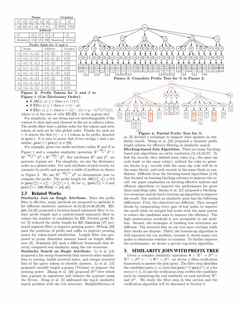
Name Country
e11 e12 e13 e14 e15 e16 ...
an do ef en er fe ...
e31 e32
ENG USA
Address
e21 e22 e23 e24 e25 e26
Berkeley CA CS EE Stanford UCLA
Prefix Table for R and SName Address Country
r1 {e11, e13, e
15} {e24, e
26} {e32}
r2 {e12, e14, e
15} {e22, e
23, e
25} {e32}
r3 {e11, e15, e
111} {e21, e
23} {e31}
r4 {e11, e13, e
15} {e22, e
23, e
25} {e32}
r5 {e11, e12, e
14} {e22, e
23, e
25} {e32}
s1 {e11, e13, e
15} {e25, e
22} {e32}
s2 {e11, e15, e
110} {e21, e
22} {e31}
s3 {e12, e14, e
15} {e21, e
23} {e31}
Figure 2: Prefix Tokens for R and S inFigure 1 (Use Dictionary Order).
r4r5
LR4
root
e12 e13 e14 e15 e111
e22 e23 e24 e25 e26
r4r5
r3 r4r5
r1
e22 e23 e25
r2r5
r2r5
e22 e23 e25
r4r4 r4
e22 e23 e25
r2r5
e22 e23 e25 e21 e23
LR10LR
2 LR3 LR
6 LR7 LR
9 LR11 LR
12 LR14 LR
16
r2r5
LR17
r2r5
LR18
r2r4
LR20
r3
LR21
r2r4
LR24
r3
LR26
r3
LR27
e32 e31 e32 e32 e32 e32 e32 e32 e32 e32 e32 e32 e32 e32 e31 e32 e31 e31
r1
LR5
e32
r2r5
LR8
e32
e26
e32
r1
LR15
e26
e32
r1
LR25
e24
r1
LR13
e32
e24
e32
r1
LR23
e21
r3
LR1
e31
e21
e31
r3
LR19
e32
r2r4
LR22
e11
Figure 3: Complete Prefix Tree for R in Figure 2.
• If JAC(r, s) � ⌧ then o = d⌧ |r|e.• If ED(r, s) ⌧ then o = |r|� q⌧ .
• If ES(r, s) � ⌧ , then o = d|r|� (|r|+ q � 1) (1�⌧)
⌧
|r|)e.where |r| is the size of r(for ED/ES, r is the q-gram set).
For simplicity, we use string and set interchangeably if thecontext is clear and each element in the set is called a token.The prefix filter fixes a global order for the tokens and sortstokens of each set by this global order. Finally for each setr, it selects the first |r|� o+ 1 tokens as its prefix, denotedas pre(r). It is easy to prove that if two strings r and s aresimilar, pre(r) \ pre(s) 6= � [29].
For example, given two multi-attribute tables R and S in
Figure 1 and a complex similarity operation R1
ED,1⇠ S1 ^R2
JAC,0.3⇠ S2 ^ R3
OLP,1⇠ S3. For attributes R1 and S1, wegenerate 2-gram set. For simplicity, we use the dictionaryorder as a global order. For each attribute of each record, wecompute its prefix and generate a table of prefixes as shown
in Figure 2. We use R2
JAC,0.3⇠ S2 to demonstrate how tocompute the prefix. The prefix length for JAC(r2
p
, s
2
q
) � 0.3is |pre(r2
p
)| = |r2p
|� d|r2p
|⌧e+1. So for r2
, |pre(r21
)| = 2 andpre(r2
1
) = {EE, UCLA} = {e24, e26}.
2.3 Related WorksSimilarity Join on Single Attribute. Since the prefixfilter is e↵ective, many methods are proposed to optimize itfor di↵erent similarity operators [6,16,20,24,26,28,29]. ED-join [12,28] proposed a location-based mismatch filter to re-duce prefix length and a content-based mismatch filter toreduce the number of candidates for ED. Pivotal prefix fil-ter [4] reduced the prefix length for ED. PassJoin [17] pro-posed segment filter to improve pruning power. PPJoin [29]used the positions of prefix and su�x to improve pruningpower for token-based similarities. Length filter was pro-posed to prune dissimilar answers based on length di↵er-ence [8]. TrieJoin [23] used a di↵erent framework that di-rectly computed real similarity using the trie structure.Similarity Search on Single Attribute. Li et al. [14]proposed a list-merge framework that converts other similar-ities to overlap, builds inverted index, and merges invertedlists of the query tokens to identify answers. Li et al. [15]proposed variable length q-grams (VGram) to improve thepruning power. Zhang et al. [30] proposed B
ed-tree whichuses q-grams as signatures and indexes the q-grams usingthe B-tree. Deng et al. [5] addressed the top-k similaritysearch problem with the trie structure. Hadjieleftheriou et
r4r5
L4
root
an do ef en er er
CA CS EE Stanford UCLA
r4r5
r3
r4r5
r1
r2r5
L8
L2
L3
L6 L7
r2r5
L10
r2r4
L12r2r4
L15
r3
L17
h1 h2r1
L5r1
L16
r1r4
L9
r1
L14
Berkeley
r3
L1
r3
L11r2r3r4
L13
CA CS EE Stanford UCLABerkeley
Figure 4: Partial Prefix Tree for R.al. [9] devised a technique to support data updates in sim-ilarity search. Wang et al. [25] proposed a dynamic prefixlength scheme for e↵ective filtering in similarity search.Blocking-based Join Algorithm. There are many blocking-based join algorithms on entity resolution [11,13,19,27]. Tolink the records, they defined some rules (e.g., the same zipcode leads to the same entity), utilized the rules to gener-ate blocks (e.g., records with the same zip code will be inthe same block), and took records in the same block as can-didates. Di↵erent from the blocking-based algorithms [3,18]that focused on learning blocking schemes to improve the re-call, our paper emphasizes on devising e↵ective indexes ande�cient algorithms to improve the performance for givenfuzzy-matching rules. Sarma et al. [21] proposed a blocking-tree structure and devised a bottom-up algorithm to improvethe recall. Our method on similarity joins has the followingdi↵erences. First, the objectives are di↵erent. They mergedblocks by enumerating every pair of leaf nodes to improvethe recall while we merged leaf nodes with the same parentto reduce the candidate sizes to improve the e�ciency. Thehigh enumeration overhead is not acceptable in our prob-lem. Second, the strategies of building tree structures aredi↵erent. The inverted lists on our tree have overlaps whiletheir blocks are disjoint. Third, the bottom-up algorithm isstill expensive for our problem, because it checks many treenodes to determine whether to combine. To further improvethe performance, we devise a greedy top-down algorithm.
3. SIMILARITY JOIN WITH PREFIX TREEGiven a complex similarity operation � = Ri1 ⇠ Sj1 ^
Ri2 ⇠ Sj2 ^ · · · ^Rik ⇠ Sjk , we devise a filter-verificationframework to answer the join query. The filter step identifiesthe candidate pairs hr, si such that pre(rit)\pre(sjt) 6= � forevery t 2 [1, k] and the verification step verifies the candidateparis by computing the real similarity on each attribute Rit
and Sjt . We study the filter step in this section and theverification algorithm will be discussed in Section 5.

Algorithm 1: PrefixTree-Join (R, S, �)Input: R, S: Two multi-attribute tables
�: A complex similarity operationOutput: A: AnswerBuild one prefix tree with two tables R and S;1
for each leaf node do2
if there are two inverted lists LR and LS then3
for each (r, s) 2 LR ⇥ LS do4
Verify(r, s);5
if r is similar to s then6
Add hr, si to A;7
3.1 Prefix TreeTo e�ciently identify the candidates, we build a com-
plete prefix tree. Given a similarity operation �, we firstsort the predicates in �. Suppose the sorted predicates areRi1 ⇠ Sj1 ^ Ri2 ⇠ Sj2 ^ · · · ^ Rik ⇠ Sjk (the details onsorting the attributes will be discussed in Section 3.2.3). Forsimplicity, we first discuss how to construct a complete prefixtree for R with the attribute order Ri1
,Ri2, · · · ,Rik as fol-
lows. For each record r 2 R, each prefix token combinationhe1, e2, · · · , eki where e
t 2 pre(rit) corresponds to a pathfrom the root to a leaf node, and each token e
t correspondsto a tree node. At the leaf node, we keep an inverted list ofrecords that contain this token combination. For example,Figure 3 shows the complete prefix tree for R in Figure 2.
Next we discuss how to utilize the complete prefix treeto support similarity joins. We extend the complete prefixtree to support two tables, where two inverted lists on eachleaf node l are maintained, LR
l
for R and LSl
for S. Foreach record r 2 R, we append it to the inverted list LR ofthe corresponding leaf node, and for each record s 2 S, weappend it to inverted list LS . Obviously, for each leaf nodel, the pair (r, s) 2 LR
l
⇥ LSl
must be a candidate becauser and s share a prefix token on every predicate. On theother hand, if (r, s) is a candidate, they must appear on theinverted lists of the same leaf node, because the completeprefix tree contains all prefix token combinations.Algorithm 1 shows the pseudo-code. PrefixTree-Join
first constructs one prefix tree for tables R and S, and agiven predicate order of the complex similarity operation �(line 1). On each leaf node, it maintains two inverted lists:LR for R and LS for S. Then it identifies all leaf nodes,and for each leaf node, if there are two inverted lists (line 3),it enumerates the candidate pairs in these two lists (line 4).Next it verifies them (line 5), and if they are actually similar,it adds this pair to the result set (line 7).For example, given two tables R and S with a complex
similarity operationR3
OLP,1⇠ S3^R2
JAC,0.3⇠ S2. We first con-struct a complete prefix tree as shown in Figure 5. Then weenumerate all leaf nodes to generate candidate pairs. Takethe leaf node e
2
1
as an example. We add the pairs from itstwo inverted lists LR
1
⇥ LS1
, i.e., {(r3
, s
2
), (r3
, s
3
)}, to thecandidate set. Finally, there are 9 candidate pairs. If we usethe brute-force enumeration, there are 3 · 5 = 15 candidatepairs. After verification, the results are {(r
4
, s
1
), (r3
, s
2
)}.However the complete prefix tree has a rather large index
size (see space complexity in Appendix D), because it re-quires to enumerate every token combination for each record,especially for records with long prefixes. To address this is-sue, we propose a partial prefix tree which is a shrunk com-plete prefix tree. Di↵erent from complete prefix tree, we donot maintain every path. Instead, we select some subtrees
root
e21
e32e31
s2s3
LS1
r3
LR1
s1
LS4
r2r4r5
LR4
e22 e25
s1
LS7LR
7
r2r4r5
e23
s3
LS3
r3
LR3
e22 e23 e24 e26
s2
LS2 LR
6
r1
LR8
r1r2r4r5
LR5 LS
5 LS6LR
2 LS8
Figure 5: Prefix Tree for Tables R and S in Figure 2(LR(LS): inverted list for R (S)).and for each subtree, we shrink it as a leaf node, and mergethe inverted lists of its leaf descendants as the inverted listof the new leaf node.
For example, Figure 4 shows a partial prefix tree for Rin Figure 2. Compared to the complete prefix tree in Fig-ure 3, the partial prefix tree shrinks the subtrees rootedat {e1
2
,e13
,e14
,e111
} and removes many unnecessary branches.Obviously the partial prefix tree is much smaller than thecomplete prefix tree since the partial prefix tree does notmaintain every token combination. However there may bemany possible partial prefix trees and next we discuss howto construct an optimal partial tree.
3.2 Optimal Prefix TreeFor simplicity, we use prefix tree and partial prefix inter-
changeably if the context is clear. To construct an optimalprefix tree, we first define a cost model to evaluate a prefixtree in Section 3.2.1. Then we discuss how to construct anoptimal prefix tree with a specific predicate order in Sec-tion 3.2.2. Next, we prove that the problem of selectingthe optimal predicate order is NP complete and propose agreedy algorithm in Section 3.2.3.
3.2.1 Join Cost Model with Prefix TreeSince the join algorithm enumerates all pairs in the two
inverted lists, our goal is to minimize the Cartesian productof the inverted lists. Next we define the cost model.
Definition 3 (Prefix tree Join Cost). Given a pre-fix tree T built with two tables R and S, the join cost is
⇥(T ) =X
l2Leaf(T )
|LRl
||LSl
|costv
(1)
where Leaf(T ) is the leaf node set of the prefix tree, LRl
andLS
l
are respectively the inverted lists of R and S on the leafnode l and cost
v
is the average cost of verifying a candidate.
For example, consider the prefix tree built with tables Rand S in Figure 5. The join cost of prefix tree ⇥(T ) =P
8
i=1
|LRi
||LSi
|costv
= 9 ⇤ costv
. 1
Then we define the optimal prefix tree.
Definition 4. (Optimal Prefix Tree with A Pred-icate Order) Given a similarity operation with a predicateorder and two tables R and S, a partial prefix tree is an opti-mal prefix tree with the predicate order if it has the minimumjoin cost among all prefix trees with this predicate order.
For example, Figure 6 shows an optimal prefix tree of thecomplete prefix tree in Figure 5.1
Our cost model does not consider the duplicate candidate pairs indi↵erent leaf nodes. For example, (r4, s1) will be counted 2 times un-der di↵erent leaves in Figure 5. In practice, we only verify a candidatepair once by utilizing a hash table to avoid the duplicate verification.

Algorithm 2: Optimal-BottomUp (R, S, �, ⇡)Input: R, S: Two multi-attribute data tables
�: A sorted complex similarity operationOutput: T : Optimal prefix treeConstruct a complete prefix tree T with R,S and �;1
for each node v 2 T from bottom to top do2
if v is a leaf then ⇥(v) = |LRv
||LSv
| else3
LRv
= [c2Child(v)LR
c
;4
LSv
= [c2Child(v)LS
c
;5
ifP
c2Child(v)⇥(c) < |LRv
||LSv
| then6
⇥(v) =P
c2Child(v)⇥(c) ;7
else8
⇥(v) = |LRv
||LSv
| ;9
Mark v as leaf and remove its children;10
return T ;11
root
e32e31
s2s3
LS1
r3
LR1
s1
LS2LR
2
r2r4r5
Figure 6: Optimal Prefix Tree for Tables R and S.3.2.2 Optimal Prefix Tree with A Predicate OrderGiven a complex similarity operation with a specified or-
der of predicates, we show how to construct an optimal prefixtree with the minimum join cost. The basic idea is that wefirst build a complete prefix tree and then determine if wecombine some paths in the complete prefix tree in a bottom-up manner based on the join cost model. We devise a two-step algorithm to construct the optimal prefix tree as shownin Algorithm 2. In the first step, it constructs a completeprefix tree given a specific predicate order (line 1). In thesecond step, it revisits nodes from bottom to top to prunesubtrees (line 3). When checking each node, it comparesthe cost of the subtree (|LR
v
||LSv
|) and the cost of merg-ing its children (
Pc2Child(v)⇥(c))
2. If the latter is smaller,we keep its children (line 7); otherwise we merge its chil-dren(lines 9-10). As it visits nodes in a bottom-up manner,it guarantees the subtree rooted at each node is optimal.
For example, given two tables R and S in Figure 1, and
a complex similarity operation with an order R3
OLP,1⇠ S3 ^R2
JAC,0.3⇠ S2. We first construct the complete tree as shownin Figure 5. Then we enumerate all the nodes from bottomto top to prune branches. Taking node e
3
1
as an example,the cost of its subtree is |LR
1
||LS1
|+ |LR2
||LS2
|+ |LR3
||LS3
| = 3,which is larger than the merging cost |LR
1
[LR2
[LR3
||LS1
[LS
2
[ LS3
| = 2. Thus we remove the children of e31
and marke
3
1
as a leaf node. Similarly, we prune the subtree of node e
3
2
and all nodes with an empty list and construct an optimalprefix tree as shown in Figure 6. The join cost with theoptimal prefix tree is 5 while that of the complete tree is 9.The Optimal-BottomUp algorithm can find the optimal
tree correctly as shown in Lemma 1.
Lemma 1. The partial tree built by Optimal-BottomUpis an optimal prefix tree with the given predicate order.
2For ease of presentation we omit the same coe�cient costv
Algorithm 3: Greedy-TopDown (R, S, �)Input: R, S: Two multi-attribute tables
�: A sorted complex similarity operationOutput: T : A prefix treeInitialize F with (root, �
1
); /* �1
: the 1st operation*/1
for each (v,�i
) 2 F do2
Split v to generate children Child(v) with �i+1
;3
ifP
c2Child(v) |LRc
||LSc
| < |LRv
||LSv
| then4
Add all (c, �i+1
) to F for each c 2 Child(v);5
else6
Mark v as a leaf;7
return T ;8
Though Algorithm 2 can build the optimal prefix treewith a specified ordered complex similarity operation, itsconstruction cost is expensive (see the complexity in Ap-pendix D). To address this issue we propose a greedy al-gorithm to construct a partial prefix tree. Di↵erent fromthe optimal solution which directly builds the complete pre-fix tree, we construct a prefix tree in a top-down manner.For each node, we compare the cost of splitting the subtreerooted at it and that of not splitting the subtree. If the for-mer is better, we split the node; otherwise we take it as aleaf node. The pseudo-code is shown in Algorithm 3. Givena complex operation �, it first initializes a queue F with theroot and the first similarity predicate �
1
(line 1). Then foreach record in the queue F , it splits the node and generatesits children (line 3). If
Pc2Child(v) |LR
c
||LSc
| < |LRv
||LSv
|, itsplits the node and adds its children into F (line 5); other-wise, it takes this node as a leaf node (line 7).
For example, consider the prefix tree in Figure 5. Givennode e1
3
, the cost of splitting node e13
is |LR1
||LS1
|+|LR2
||LS2
| =3, and the cost of not splitting node e
1
3
is |LR1
[ LR2
||LS1
[LS
2
| = 2. Thus we do not split e13
.
3.2.3 Optimal Prefix Tree without A Predicate OrderGiven a similarity operation with |�| atomic predicates,
there are |�|! predicate order, and for each order, there isan optimal prefix tree. We would like to find the optimalprefix tree among these prefix trees.
Definition 5. (Optimal Prefix Tree) Given a sim-ilarity operation and two tables R and S, a partial prefixtree is an optimal prefix tree if it has the minimum join costamong all partial prefix trees.
However, the problem of finding the optimal prefix tree isNP-Hard as formalized in Lemma 2.
Lemma 2. Given two tables R and S, a complex similar-ity operation �, finding the optimal prefix tree is NP-Hard.
Since find the optimal prefix tree is NP-Hard, we proposean approximation algorithm. We first evaluate the cost ofeach predicate on the whole table as follows
Cost(�i
) =X
c2Child(root)
|LRc
||LSc
| (2)
where �i
is the i
th operation of �. Then it sorts the predi-cates by Cost(�
i
) and constructs a prefix tree based on thesorted order. For example, given tables in Figure 1 and a
complex operation R1
ED,1⇠ S1 ^R2
JAC,0.3⇠ S2 ^R3
OLP,1⇠ S3.We first evaluate the cost of each predicate. The size of theinverted list built with �
3
is |LR1
| = 1, |LS1
| = 2, |LR2
| =4, |LS
2
| = 1. Cost(�3
) =P
2
c=1
|LRc
||LSc
| = 6. Similarly, wecomputeCost(�
2
) = 15 andCost(�1
) = 26. AsCost(�3
) <Cost(�
2
) < Cost(�1
), the predicate order is h�3
,�2
,�1
i.
4. SIMILARITY SEARCH WITH PREFIX TREEWe extend the prefix tree to support similarity search
on multi-attribute data. We first give an overview in Sec-tion 4.1. Then we discuss how to utilize the prefix tree toanswer a search query in Section 4.2. Finally we propose tobuild the prefix trees for similarity search in Section 4.3.
4.1 OverviewFor a similarity join query, the cost of constructing a prefix
tree is less than the join cost. However for a similarity searchquery, the construction cost is much more expensive thanthe cost of answering a search query. Thus for a similaritysearch query, we want to construct the prefix tree o✏ine soas to utilize it to answer online search queries. To utilizeprefix trees to support similarity search queries, we need toanswer the following questions.
First, di↵erent search queries have various similarity func-tions and thresholds. For example, given the table in Fig-ure 1, a user is familiar with the address but is not sure
how to spell the name, and issues a query (NameES,0.6⇠
‘Jenifer Ullman’, AddressJAC,0.8⇠ ‘CS Stanford’). An-
other user knows the name but is not familiar with the ad-dress, and issues a query (Name
ES,0.9⇠ ‘Jeffery Ullman’,
AddressJAC,0.7⇠ ‘EE Stanford’). Obviously the two queries
involve di↵erent functions and thresholds. Since the prefixesdepend on the similarity functions and thresholds, can westill use prefix trees to support similarity search? The an-swer is yes. A common technique is to set a smallest possiblesimilarity threshold that a system can tolerate, e.g., 0.6, andwe utilize this threshold to construct prefix trees. An alter-native is to build delta prefix trees. That is we build a prefixtree for each threshold range, e.g., [1, 0.9], (0.9, 0.8], (0.8, 0.7],(0.7, 0.6]. Given a query threshold 0.8, we use the first twoprefix trees to answer the query. For simplicity, we take thefirst method as an example. To support various functions,we transform them to the overlap similarity and use thesmallest threshold o to generate the prefix (see Section 2.2).
Second, since there are many search queries and di↵er-ent queries involve di↵erent attribute combinations, a singleprefix tree cannot e�ciently answer all search queries andwe have to construct multiple prefix trees to answer searchqueries. There are two issues we need to address. Thefirst is how to construct multiple high-quality prefix treesto answer search queries? Since search queries are not givenand di↵erent queries have di↵erent similarity functions andthresholds, the cost model for similarity joins cannot sup-port search queries. To address this issue, we propose anew model to support similarity search in Section 4.3. Thesecond is that given multiple prefix trees, how to e�cientlyutilize them to answer a search query? We propose e�cientalgorithms to address this issue in Section 4.2.
Based on these questions, we devise a framework to sup-port similarity search queries on multi-attribute data. Firstwe construct multiple prefix trees o✏ine (see Section 4.3).Then given an online query, we devise e�cient algorithms toanswer the query using these prefix trees (see Section 4.2).
4.2 Prefix-Tree-Based Search AlgorithmsUsing A Single Prefix Tree T to Answer A QueryQ. If the first-level attribute of T appears in Q, we canuse T to answer Q. The basic idea is to find the leaf nodesof T such that the tokens on the path from the root to
root
e32e31
r3
LR1
r1r2r4r5
LR2
root
e13 e15e12 e14e11
r2r5
LR2
r3
LR6
r1r3r4r5
LR1
r1r4
LR3
r2r5
LR4
r1r2r3r4
LR5
e111
root
e23 e25e22 e24 e26e21
r2r4r5
LR2
r2r4r5
LR4
r2r4r5
LR6
r3
LR1
r3
LR3
r3
LR5
r3
LR7e31 e32
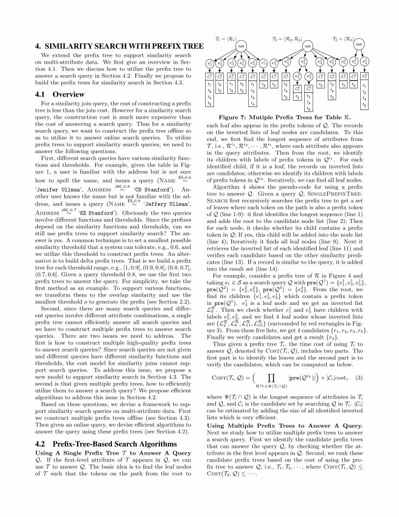
T1 = hR1i T2 = hR2,R3i T3 = hR3i
Figure 7: Mutiple Prefix Trees for Table R.
each leaf also appear in the prefix tokens of Q. The recordson the inverted lists of leaf nodes are candidates. To thisend, we first find the longest sequence of attributes fromT , i.e., Ri1
,Ri2, · · · ,Rit , where each attribute also appears
in the query attributes. Then from the root, we identifyits children with labels of prefix tokens in Qi1 . For eachidentified child, if it is a leaf, the records on inverted listsare candidates; otherwise we identify its children with labelsof prefix tokens in Qi2 . Iteratively, we can find all leaf nodes.
Algorithm 4 shows the pseudo-code for using a prefixtree to answer Q. Given a query Q, SinglePrefixTree-Search first recursively searches the prefix tree to get a setof leaves where each token on the path is also a prefix tokenof Q (line 1-9): it first identifies the longest sequence (line 1)and adds the root to the candidate node list (line 2); Thenfor each node, it checks whether its child contains a prefixtoken in Q; If yes, this child will be added into the node list(line 4); Iteratively it finds all leaf nodes (line 9). Next itretrieves the inverted list of each identified leaf (line 11) andverifies each candidate based on the other similarity predi-cates (line 13). If a record is similar to the query, it is addedinto the result set (line 14).
For example, consider a prefix tree of R in Figure 4 andtaking s
1
2 S as a search queryQ with pre(Q1) = {e11
, e
1
3
, e
1
5
},pre(Q2) = {e2
2
, e
2
5
}, pre(Q3) = {e32
}. From the root, wefind its children {e1
1
, e
1
3
, e
1
5
} which contain a prefix tokenin pre(Q1). e
1
3
is a leaf node and we get an inverted listLR
9
. Then we check whether e
1
1
and e
1
5
have children withlabels e
2
5
, e
2
2
, and we find 4 leaf nodes whose inverted listsare {LR
2
,LR6
,LR11
,LR15
} (surrounded by red rectangles in Fig-ure 3). From these five lists, we get 4 candidates {r
1
, r
2
, r
4
, r
5
}.Finally we verify candidates and get a result {r
4
}.Thus given a prefix tree T
i
, the time cost of using Ti
toanswer Q, denoted by Cost(T
i
,Q), includes two parts. Thefirst part is to identify the leaves and the second part is toverify the candidates, which can be computed as below.
Cost(Ti
,Q) =⇣ Y
Rjk2 (Ti\Q)
|pre(Qjk )|⌘+ |C
i
|costv
(3)
where (Ti
\Q) is the longest sequence of attributes in Ti
and Q, and Ci
is the candidate set by searching Q in Ti
. |Ci
|can be estimated by adding the size of all identified invertedlists which is very e�cient.
Using Multiple Prefix Trees to Answer A Query.Next we study how to utilize multiple prefix trees to answera search query. First we identify the candidate prefix treesthat can answer the query Q, by checking whether the at-tribute in the first level appears in Q. Second, we rank thesecandidate prefix trees based on the cost of using the pre-fix tree to answer Q, i.e., T
1
, T2
, · · · , where Cost(T1
,Q) Cost(T
2
,Q) · · · .

Algorithm 4: SinglePrefixTree-Search (T , Q, �)
Input: T : Prefix treeQ: Search query�: A complex similarity operation
Output: A: Answer setIdentify the longest sequence of attributes1
Ri1,Ri2
, · · · ,Rit of T that also appear in Q;NodeSet = {root};2
for j = 1 to t do3
for node in NodeSet do4
NodeSet0 = �;5
for e
j in prefix of Qij do6
if node has a child n
j
with label ej then7
if n
j
is a leaf then LeafSet n
j
else8
NodeSet0 n
j
NodeSet = NodeSet0;9
for each leaf l 2 LeafSet do10
Retrive its inverted list L(l);11
for each candidate c 2 L(l) do12
Verify (c, Q);13
if c is simlar to Q then Add c to A;14
Then we have two strategies to answer the query. Thefirst one is that we use the prefix tree T
1
with the minimumcost to generate a candidate set C
1
and verify the candi-dates using other attributes. The second one is that weutilize another tree T
i
to identify another candidate set Ci
and intersect C1
and Ci
. Based on the new candidate setC1
\ Ci
, we can still utilize these two strategies to computethe answer. Iteratively, we can find all the results.
Next we define a cost model to select a better strategy.The cost of the first strategy is
Cost1
= Cost(T1
,Q). (4)
The cost of the second strategy is
Cost2
=Y
Rjk2 (T1\Q)
|pre(Qjk )|+Y
Rjk2 (Ti\Q)
|pre(Qjk )|
+ |C1
|+ |Ci
|+ |C1
\ Ci
|costv
.
(5)
where |C1
\ Ci
| can be obtained through sampling.If Cost
1
Cost2
, we select the first strategy; otherwisewe select the second strategy.
The pseudo code is shown in Algorithm 5. It first retrievesprefix trees that can answer Q from W (line 1). Then itestimates Cost(T
i
,Q) and sorts Ti
(line 2). It estimatesthe cost of the two methods (line 4-7). If the intersection-based method is better, it intersects the two candidates anditeratively decides to verify or intersect two candidate sets(line 9-11). Otherwise, it verifies the candidates (line 12).
4.3 Multiple Prefix-Trees ConstructionThe cost of searching prefix trees depends on two factors.
The first is the query distribution, e.g. which attributes orattribute combinations are frequently searched. The secondis data distribution, e.g. some attributes have more uniquevalues than other attributes. Since we do not know thedistribution of search queries, in this paper we only considerthe data distribution.
As there are at least x prefix trees, we first build x treesusing each attribute at the first level. We can use these treesto answer any query. If there is more space, we optimize
Algorithm 5: MultiTreeSearch (R, Q, �, W)
Input: R: Multi-attribute data tableQ: Search queryW: Multiple prefix trees T
1
, T2
..Tm
Output: A: Answer setWQ {T
i
|Ti
2W,Ri1 2 Q} ;1
Sort Ti
2WQ by Cost(Ti
,Q);2
A Candidates using T1
;3
Cost1
= Cost(T1
,Q) + |C1
|costv
;4
for each Ti
2WQ do5
Estimate Cost2
(Ti
) by Equation(5) ;6
Choose Tp
with smallest Cost2
(Tp
) ;7
if Cost2
(Tp
) < Cost1
then8
Cp
Candidates using Tp
;9
A = A \ Cp
;10
Decide to verify A or further intersect;11
else Verify all records in A;12
return A;13
these prefix trees and propose a cost-based method. Nextwe define the cost and benefit of adding an attribute Rj tocurrent tree T
i
. The cost is the space increase by adding Rj
to Ti
and the benefit is query performance improvement.As the new prefix tree shares many tree nodes with T
i
, weonly consider the cost of new inverted lists by adding Rj toTi
. As each record in T appears |pre(rRj )| times in the newtree and thus the space cost can be computed as below.
CostSpace(Ti
,Rj) =X
l2Leaf(Ti)
X
r2LRl
(|pre(rRj )|) (6)
The benefit is hard to measure and di↵erent queries havedi↵erent benefits. Here our objective is to avoid slow queries,i.e., there are no rather long inverted lists on the prefix tree.Thus we want to make inverted lists evenly distributed afteradding Rj . To achieve this goal, we use a modified Shannonentropy to capture this information.
Definition 6. The entropy of prefix tree T in search is
H(T ) =X
l2Leaf(T )
�P(l) logP(l) (7)
where Leaf(T ) is the leaf set of T and P(l) is the ratio ofinverted-list size of node l to the sum of inverted-list sizes,
P(l) =|LR
l
|Pl
02Leaf(Ti)|LR
l
0 |. (8)
Obviously, the larger entropy, the smaller average searchcost of using prefix tree to answer a query. With this entropycost model, we can define the benefit of adding Rj ,
Benefit(Ti
,Rj) = H(Ti
,Rj)�H(Ti
) (9)
where H(Ti
,Rj) denotes the entropy of the new tree byadding Rj to T
i
.Using the cost and benefit, our goal is to achieve the max-
imum benefit with a given space budget B. However, thisgeneralizes the classical knapsack problem, which is NP-Hard. To this end, we devise a greedy algorithm to buildthe prefix trees. We select the attribute Rj and T
i
with the
largest value Benefit(Ti,Rj)
CostSpace(Ti,Rj)
, and insert the new tree into the
tree set. The algorithm terminates until there is no spaceto accommodate any prefix tree. Algorithm 6 shows pseudocode. It first creates one-level prefix trees for each attribute(lines 1-2). Then it greedily adds a new prefix tree (lines 6-9). It terminates when meeting the space budget (line 6).

Algorithm 6: BuildMultipleTrees (R, B)Input: R: Multi-attribute table
B: Space budgetOutput: W: A set of prefix treesfor each attribute Ri do1
Construct Ti
with Ri and add Ti
to W;2
while B > 0 do3
for each Ti
2W do4
for each Rj do5
Compute CostSpace(Ti
,Rj) with Equation 6;6
Compute Benefit(Ti
,Rj) with Equation 9;7
Expand Ti
using Rj with largest Benefit(Ti,Rj)
CostSpace(Ti,Rj)
;8
W T (Ti
,Rj);9
B B �CostSpace(Ti
,Rj) ;10
return W ;11
For example, consider adding an attribute to T1
in Fig-ure 7. If we add attributeR3, the benifit Benefit(T
1
,R3) =0.298 and the cost CostSpace(T1
,R3) = 4. Similarly we canestimate Benefit(T
1
,R2) = 1.057 and CostSpace(T1
,R2) =
39. Benefit(T1,R3)
CostSpace(T1,R3)
= 0.0745 and Benefit(T1,R2)
CostSpace(T1,R2)
= 0.0271,
As Benefit(T1,R3)
CostSpace(T1,R3)
>
Benefit(T1,R2)
CostSpace(T1,R2)
, we expend T1
with R3.
5. HYBRID VERIFICATIONIn this section, we study how to e�ciently verify a candi-
date pair. There are two challenges in verifying a pair. Thefirst is to determine the order of verifying di↵erent predi-cates. The second is to decide the order of using di↵erentfiltering algorithms. To address these challenges, we proposea hybrid verification framework and prove its optimality.
5.1 Hybrid-based Verification FrameworkGiven a complex similarity operation � and a candidate
pair hr, si, we check whether hr, si satisfies each predicate in�. A straightforward way is to examine each predicate oneby one through computing the real similarity. However thismethod has two weaknesses. First, directly computing thesimilarity is expensive. For example, the cost to verify hr, sion the token-based function is |r|+ |s| while the cost on thecharacter-based function is (2⌧ + 1) · min(|r|, |s|). Second,the pruning power of each predicate is also di↵erent andit is important to select an appropriate order of predicatesto verify candidates. For example, given a candidate pair
hr1
, s
1
i and a complex similarity operation R1
ED,1⇠ S1 ^R2
JAC,0.3⇠ S2 ^R3
OLP,1⇠ S3, if we verify them with the orderh�
1
,�3
,�2
i. The cost is (3 · 14) + (1 + 1) + (2 + 2) = 48.However, if we use the order h�
2
,�1
,�3
i, then the pair failsin predicate �
2
, and thus the cost is only 2 + 2 = 4.To reduce the verification cost, we can use lightweight
filters instead of computing the actual similarity. If the paircannot pass the filter, we prune it; otherwise we use otherfilters or compute the actual similarity. For example, thelength filter can prune those pairs with length di↵erencelarger than ⌧ for edit distance. However di↵erent filters havedi↵erent cost and pruning power and it is also important toselect an appropriate order for using filtering algorithms.
Formally, suppose a similarity operation � has k similaritypredicates �
1
,�2
, · · · ,�k
, v filters �1
,�2
, · · · ,�v
, and eachpredicate �
i
also has a best verification algorithm ⇤i
. Thereare many possible ways to verify the pair. A naive way thatdoes not use any filter is h�
1
,⇤1
i, h�2
,⇤2
i, · · · , h�k
,⇤k
i.
Algorithm 7: HybridVerification (C, Q, �, F)
Input: C: Candidate after prefix tree; Q: Search query�: A complex similarity operation,F : A set of filters and verification algorithms
Output: A: AnswerCompute and sort verification methods by ⇥(h�,�i)
P(h�,�i) ;1
for each hr, si 2 C do2
for each h�,�i do3
if (r, s) does not pass h�,�i then4
break;5
Add hr, si to A;6
Update ⇥(h�,�i)P(h�,�i) ;7
return A;8
Another solution that uses all possible filters is h�1
,�11
i,h�
1
,�12
i, · · · , h�1
,⇤1
i, h�2
,�21
i, h�2
,�22
i, · · · , h�2
,⇤2
i,h�
k
,�k1
i, h�k
,�k2
i, · · · , h�k
,⇤k
i. We require to find an or-der with the minimum cost to verify the pair. Suppose eachfilter h�
i
,�j
i (or each verification algorithm h�i
,⇤i
i) has atime cost ⇥ to preform the filter (or the algorithm) and apruning probability P to prune the pair. We discuss how tocompute the time cost and pruning ability in Section 5.2.
Given a verification sequence = {h�1
,�1
i, h�2
,�2
i, · · · },we compute its expected verification cost as follows.
Cost( ) =X
h�,�i2
⇥(h�,�i) · P
(h�,�i), (10)
where ⇥(h�,�i) is the cost to use the filter � to verify pred-icate � and P
(h�,�i) is the probability that h�,�i is usedto verify the pair given the sequence , that is the probabil-ity the verification methods before h�,�i in cannot prunethe pair, which can be computed as
P
(h�,�i) =Y
h�0,�
0i is before h�,�i
1� P(h�0,�0i), (11)
where P(h�0,�0i) is the probability that the filter �0 on �0
can prune a pair.We design a hybrid verification algorithm to address this
problem. Algorithm 7 gives the pseudo code of the algo-rithm. It first computes ⇥(h�,�i)
P(h�,�i) for each pair of filter and
attribute, and sorts them in an ascending order (line 1).Then it utilizes this order to verify each candidate pair. Ifthe candidate passes the filter, it selects the next filter orverification algorithm; otherwise terminates (lines 2 - 5). Fi-nally it adds the pair which passes all verification algorithmsto the answer set (line 6). Then it updates the expected costfor other verification methods based on Equation 11 (line 7).Iteratively, the algorithm can find a verification order.
Note that the above greedy algorithm is known to be op-timal (see e.g., [10]), and for the sake of completeness, weprovide a simple proof of this fact in Appendix C.
For example, given a filter �1
, a verification algorithm ⇤2
and two similarity predicates �1
, �2
with the following ex-pected cost ⇥(h�,�i)
P(h�,�i) . h�1
,�1
i: 1.0
0.4
= 2.5, h�1
,⇤2
i: 8.30.9
= 9.2,
h�2
,�1
i: 1.0
0.25
= 4.0, h�2
,⇤2
i: 2.20.6
= 3.7. We sort verifica-
tion methods by ⇥(h�,�i)P(h�,�i) and get an order h�
1
,�1
i, h�2
,⇤2
i,h�
2
,�1
i, h�1
,⇤2
i. Then we compute P(h�,�i| ) iterativelyby Equation (11) and get a sequence P(h�
1
,�1
i| ) = 1,P(h�
2
,⇤2
i| ) = 0.6,P(h�2
,�1
i| ) = 0.24,P(h�1
,⇤2
i| ) =0.18. ThusCost( ) =
Ph�i,�ji2 ⇥(h�i
,�j
i)·P(h�i
,�j
i| ) =2.5 · 1+ 2.2 · 0.6+ 4.0 · 0.24+ 8.3 · 0.18 = 6.274. If we chooseorder h�
1
,⇤2
i, h�2
,�1
i, h�2
,⇤2
i, h�1
,�1
i, Cost( ) = 8.64.

5.2 Verification Cost and Pruning ProbabilityWe first discuss the verification cost of various filters. Here
we only take important filters as examples. It is worth notingthat our method is orthogonal to the filtering techniques andour method can be easily extended to support any filter.
Length Filter. It prunes hr, si if their length di↵erence islarger than ⌧ for ED and |r| 1�⌧
⌧
for JAC. The time cost ⇥is O(1) for the search problem, since the length/size can bematerialized; but for the join problem, the cost is O(1) forthe attribute in the similarity operation as we can get thelength when computing the prefixes; O(|r|+ |s|) otherwise.Prefix Filter. It prunes hr, si if their prefixes have no com-mon token. The time cost ⇥ is O(pre(r) + pre(s)). (If theprefix filter is used in the filtering step for this attribute, wewill not use it again and set its pruning probability as 0.)
Count Filter. It is useful only for character-based func-tions. If two strings are similar, they must share max(|r|, |s|)�q+1� ⌧q common q grams. The time cost ⇥ is O(|r|+ |s|).Content Filter. It is useful only for character-based simi-larity functions. For example, for ED, it computes the sumof the number of character di↵erence and if the di↵erence islarger than 2⌧ , it prunes the pair. The cost is O(|r|+ |s|).
The well-known verification algorithm for ED is the dynamic-programming algorithm with time cost of O(2⌧ min(|r|, |s|)).The verification algorithm for JAC is O(|r|+ |s|).
Next we analyze the filtering probability. Initially, we canutilize a sampling-based method to compute the pruningprobability of each filter. Then, after verifying each record,we update the pruning probability of each filter. However itis not free to get the pruning probability and it is expensiveto compute an appropriate order for every pair. Instead,we periodically update the order. For similarity join, wegroup the candidates based on a record in R and use thesame order for candidates in the same group; for similaritysearch, we can use the same order for all candidates.
6. EXPERIMENTWe have implemented our techniques to support similarity
join and search on multi-attribute data and our goal is toevaluate the e�ciency. We used two real datasets DBLP andIMDB in the experiments, as shown in Table 1.DBLP: It is a publication dataset (dblp.uni-trier.de/xml/).We ran self-join on DBLP with 4 attributes {title, journal,author, year}. The similarity operation was title
COS,⌧⇠ title
^journalJAC,⌧⇠ journal^authorES,⌧⇠ author^yearES,⌧⇠ year byvarying ⌧ in [0.75, 0.95].IMDB: It is a movie database (imdb.com). We ran self-join on IMDB with 4 attributes {title, genres, director,writer}. The similarity operation was title
ES,⌧⇠ title ^genres
JAC,⌧⇠ genres ^directorES,⌧⇠ director^writerES,⌧⇠ writer
by varying ⌧ in [0.75, 0.95].All the algorithms were implemented in C++ and com-
piled using GCC 4.7 with the -O3 flag. All the experimentswere conducted on a machine running 64bit Ubuntu 14.04with Intel Xeon E2650 2.0GHz processor and 16GB RAM.
6.1 Evaluation on Prefix Trees for JoinIn this section, we evaluated our prefix trees for similar-
ity join. We first compared our optimal prefix tree and thegreedy prefix tree with CBlockTree [21], which was used tomerge blocks to improve the recall of the blocking-basedscheme (see Appendix C for details). Figure 8 shows the
Table 1: Datasets.Datasets # Records # Attributes SizeDBLP 1M 4 174MBIMDB 400K 4 159MB
candidate numbers and join time, where the bars from bot-tom to top respectively denote the time of building trees,filtering time and verification time. We had the followingobservations. First, CBlockTree reduced the number of can-didates, because it enumerated every two leaves and mergedthe leaves with the join cost on the merged node smallerthan the cost on two individual leaves, while our methodonly checked whether to combine the leaf nodes with thesame parent. However, enumerating every pair of leaf nodeshad expensive overhead, and thus CBlockTree had worseperformance than our method. Second, our greedy prefixtree nearly had the same number of candidates with the op-timal prefix tree, because if merging a subtree had a largebenefit, our greedy prefix tree would not split the subtreeand our cost model can e↵ectively decide whether to split anode or not. Third, our greedy prefix tree had much betterjoin performance than the optimal prefix tree. The reason isobvious that it took less time to construct the greedy prefixtree, and the optimal tree generated a large complete pre-fix tree and then merged many subtrees, which was rathertime consuming, especially for large datasets. Another rea-son was that the greedy tree had similar pruning power withthe optimal tree and thus it did not loss much performance.
Then, we compared di↵erent orders of predicates in con-structing the prefix trees. We compared the random orderwith our greedy order. Figure 9 shows the results. We cansee that our greedy order significantly outperformed the ran-dom order, even by 1-2 orders of magnitude. This is becauseif we used predicates with large cost in top levels, then bothindexing and filtering took much time. Our greedy algo-rithm selected an appropriate order of predicates and madeinverted lists on leaf nodes much shorter. For example, onDBLP, for ⌧ = 0.8, the random order took nearly 1000 sec-onds while our greedy order took less than 80 seconds.
6.2 Evaluation on Prefix Trees on SearchWe generated 100K search queries based on the same simi-
larity operations, varied the thresholds, and reported the av-erage search time. To build prefix index, we set a thresholdbound (0.7) for each predicate and built our multiple prefixtrees with the bound. We first evaluated our techniques byusing multiple prefix trees to answer a query (proposed inSection 4.2). Suppose the size of the multiple prefix tree withthe first level was 1. We set B = 2 in this experiment. Weimplemented three methods. (1) Intersection-based Method:It computed the candidates using each predicate and thenintersected them. (2) Pipeline-based Method: It selected thebest predicate and utilized this predicate to generate can-didates. (3) Cost-based Method: It used our cost model togenerate the candidates. Figure 10 shows the results (bot-tom/top bars denote filtering/verification time).
We had the following observations. First, on DBLP, thepipeline-based method was better than the intersection-basedmethod, because the pipeline-based method first used a highlyselective attribute to identify less candidates and then ver-ified the candidates, and thus achieved rather high per-formance. However, the intersection-based method usedeach predicate to identify many candidates and thus was
expensive. For example, consider a query (AuthorES,0.8⇠
‘Dieter Baum, Vladimir V. Kalashnikov’, JournalJAC,0.8⇠

1e+06
1e+07
1e+08
0.95 0.9 0.85 0.8 0.75
Candid
ate
Num
ber
Threshold
GreedyPrefixTreeOptimalPrefixTree
CBlockTree
(a) Candidate Number (DBLP)
1e+06
1e+07
1e+08
1e+09
0.95 0.9 0.85 0.8 0.75
Candid
ate
Num
ber
Threshold
GreedyPrefixTreeOptimalPrefixTree
CBlockTree
(b) Candidate Number (IMDB)
0
50
100
150
200
250
0.95 0.9 0.85 0.8 0.75
Tim
e(s
)
Threshold
GreedyPrefixTreeOptimalPrefixTree
CBlockTree
(c) E�ciency (DBLP)
0
200
400
600
800
1000
1200
1400
0.95 0.9 0.85 0.8 0.75
Tim
e(s
)
Threshold
GreedyPrefixTreeOptimalPrefixTree
CBlockTree
(d) E�ciency (IMDB)Figure 8: Evaluation on Prefix Trees for Similarity Join: Optimal vs Greedy vs CBlockTree
10
100
1000
0.95 0.9 0.85 0.8 0.75
Tim
e(s
)
Threshold
GreedyOrderRandomOrder
(a) E�ciency (DBLP)
10
100
1000
0.95 0.9 0.85 0.8 0.75
Tim
e(s
)
Threshold
GreedyOrderRandomOrder
(b) E�ciency (IMDB)Figure 9: Evaluation on Predicate Order for Join
0
1
2
3
4
5
0.95 0.9 0.85 0.8 0.75
Tim
e(m
s)
Threshold
CostBasedSearchSearch-Pipeline
Search-Intersection
(a) E�ciency (DBLP)
0
0.2
0.4
0.6
0.8
1
0.95 0.9 0.85 0.8 0.75
Tim
e(m
s)
Threshold
CostBasedSearchSearch-Pipeline
Search-Intersection
(b) E�ciency (IMDB)Figure 10: Evaluation on Prefix Trees for Search.
‘University Trier, Mathematik/Informatik’). Attributejournal only generated 300 candidates (by prefix filter-ing), while attribute author generated over 10K candi-dates. The intersection-based method identified 10K can-didates from attribute author and 300 candidates fromjournal while the pipeline-based method only identified300 candidates and then verified them. Obviously, the latterwas faster. Second, on IMDB, the intersection-based methodwas better than the pipeline-based method because everypredicate generated nearly the same number of answers andthe intersection-based method can further reduce the can-didate number by intersecting them, which had lower costthan directly verifying each candidate. For example, a querygenerated 1000 candidates on attribute Title and 1000 can-didates on attribute Director, and there were 100 results.The pipeline-based method identified 1000 candidates andverified 1000 candidates while the intersection-based methodidentified 2000 candidates and verified 150 candidates (therewere 150 candidates after the intersection). As the verifica-tion cost was much more expensive than the filtering cost,the intersection-based method was better. Third, our cost-based method always achieved the best performance becauseit judiciously selected appropriate predicates to generate thecandidates. If the best predicate generated a small num-ber of candidates, it directly verified the candidates; oth-erwise it selected another predicate to further reduce thenumber of candidates. For example, on DBLP, for ⌧ = 0.75,the intersection-based method took 4.6 milliseconds for eachquery, and the pipeline-based method took 2.3 milliseconds,while our cost-based method improved it to 0.4 milliseconds.
Then we evaluated the performance by varying the givenbudget B. Suppose the size of all the 1-level prefix trees was1. We varied B in 1.0, 1.5, 2.0, 2.5, and 3.0, and evaluated
0
0.1
0.2
0.3
0.4
0.5
0.6
0.7
1.00 1.5 2.0 2.5 3.0
Tim
e(m
s)
BufferSize
BuildMultiTrees
(a) E�ciency (DBLP)
0
0.05
0.1
0.15
0.2
0.25
0.3
0.35
0.4
0.45
1.00 1.5 2.0 2.5 3.0
Tim
e(m
s)
BufferSize
BuildMultiTrees
(b) E�ciency (IMDB)Figure 11: Evaluation on Search by Varying Budgets
0
50
100
150
200
250
300
350
400
0.95 0.9 0.85 0.8 0.75
Tim
e(s
)
Threshold
HybridVerificationSortedVerification
RandomVerification
(a) E�ciency (DBLP)
0
100
200
300
400
500
600
700
800
0.95 0.9 0.85 0.8 0.75
Tim
e(s
)
Threshold
HybridVerificationSortedVerification
RandomVerification
(b) E�ciency (IMDB)Figure 12: Evaluation on Verification Algorithms.
the average search performance. Figure 11 shows the results.We can see with the increase of B, our method achievedhigher performance, this is because we can use more prefixtrees to answer search queries, which obviously can improvethe performance. Especially, if each query attribute was con-tained by a prefix tree, then the prefix tree can significantlyimprove the performance than the 1-level prefix tree.
6.3 Evaluation on Verification TechniquesWe evaluated our verification techniques. We compared
three methods. (1) Random Verification: we randomly veri-fied a candidate. (2) Sorted Verification: we sorted the pred-icates based on our techniques in Section 5.1. (3) HybridVerification: we used our cost model in Section 5.1 to verifya candidate. We used the length filter, prefix filter, countfilter, and content filter in the experiment. Figure 12 showsthe results. We can see that the hybrid verification outper-formed the other two methods. This is because our hybridverification method always judiciously selected appropriateorders of predicates to verify a candidate and used the ap-propriate filtering algorithms to prune dissimilar pairs. Ourhybrid verification algorithm was better than the sorted ver-ification method, especially for a small threshold. This is be-cause selecting a predicate order was not enough to achievehigh performance and our hybrid verification method canalso utilize lightweight filters to prune many candidates. Forexample, our method can utilize the length filter and countfilter on some attributes to prune many candidate with lit-tle cost. The improvement of our hybrid method over thesorted-based method on IMDB was significant because therewere many candidates in IMDB and our hybrid can utilize dif-ferent filters to e↵ectively prune these candidates. However,on DBLP, there were few candidates using an appropriatepredicate and thus the improvement was not significant.

10
100
1000
10000
0.95 0.9 0.85 0.8 0.75
Tim
e(s
)
Threshold
PrefixTreePipeline
Intersection
2Selective2Concatenate
(a) Varying ⌧ (DBLP)
10
100
1000
10000
0.95 0.9 0.85 0.8 0.75
Tim
e(s
)
Threshold
PrefixTreePipeline
Intersection
2Selective2Concatenate
(b) Varying ⌧ (IMDB)
100
1000
10000
100000
2 3 4
Tim
e(s
)
Similarity predicate Number
PrefixTreePipeline
Intersection
2Selective2Concatenate
(c) Varying # Predicates(DBLP)
100
1000
10000
100000
2 3 4
Tim
e(s
)
Similarity predicate Number
PrefixTreePipeline
Intersection
2Selective2Concatenate
(d) Varying # Predicates(IMDB)Figure 13: Comparison on Similarity Joins.
6.4 Comparison with BaselinesWe compared our method with state-of-the-art q-gram-
based methods, PPJoin [29] for token-based similarity andED-join [28] for character-based similarity. For fair compar-ison, we used the same filters with these two algorithms,including length filter, count filter, content filter, and prefixfilter. We extended them and took them as baseline ap-proaches (see Appendix C for details): (1) Intersection:It used PPJoin or ED-join to identify the candidates on ev-ery predicate, intersected the candidates, and verified theintersected candidates. (2) Pipeline: It selected the bestpredicate using our model and used PPJoin or ED-join toidentify the candidates, and then verified the candidates.(3) 2Selective: It first identified candidates for two mostselective attributes and then intersected them. (4) 2Con-catenate: It concatenated two selective attributes as a sin-gle attribute and then used PPJoin or ED-join to identify thecandidates. We also extended them to support search by us-ing the threshold 0.7 (which was the same as our method).
6.4.1 Comparison on Similarity JoinsWe compared the performance by varying the thresholds
and the number of similarity predicates, and the result isshown in Figure 13. We had the following observations.First, with the decrease of ⌧ , the performance of all themethods become worse because a small threshold will gener-ate more results and thus all the algorithms generated morecandidates and involved more verification time. Second, thequery with more predicate numbers may not have worse per-formance, because a “lightweight” attribute will improve theperformance. For example, on DBLP, answering the querywith attributes title, journal, author was easier than an-swering query with attributes title, author, because theattribute journal can prune many dissimilar pairs. Third,the intersection-based method was always worse because itwas very expensive to identify candidates for every predi-cate. Fourth, 2Concatenate achieved the lowest perfor-mance because it generated many more candidates than In-tersection. Actually, the candidate set obtained by con-catenating two attributes is a super set of the candidate setobtained by intersecting two attributes, because if r is acandidate of intersecting two attributes, then the concate-nated attribute of r must satisfy the combined constraintand thus r is a candidate of concatenating two attributes(see Appendix C for more details). Fifth, alghouth 2Se-
0
5
10
15
20
25
30
0.95 0.9 0.85 0.8 0.75
Tim
e(m
s)
Threshold
PrefixTreePipeline
Intersection2Selective
2Concatenate
(a) Varying ⌧ (DBLP)
0.5
1
1.5
2
2.5
3
3.5
4
0.95 0.9 0.85 0.8 0.75
Tim
e(m
s)
Threshold
PrefixTreePipeline
Intersection2Selective
2Concatenate
(b) Varying ⌧ (IMDB)
0.01
0.1
1
10
100
2 3 4
Tim
e(m
s)
Similarity predicate number
PrefixTreePipeline
Intersection2Selective
2Concatenate
(c) Varying # Predicates(DBLP)
0.01
0.1
1
10
100
2 3 4
Tim
e(m
s)
Similarity predicate number
PrefixTreePipeline
Intersection2Selective
2Concatenate
(d) Varying # Predicates(IMDB)
0
5
10
15
20
25
1 1.5 2.0 2.5 3.0
Tim
e(m
s)
Buffer Size
PrefixTreePipeline
Intersection
2Selective2Concatenate
(e) DBLP
0.5
1
1.5
2
2.5
3
3.5
4
1 1.5 2.0 2.5 3.0
Tim
e(m
s)
Buffer Size
PrefixTreePipeline
Intersection
2Selective2Concatenate
(f) IMDBFigure 14: Comparison on Similarity Search withBaselines (Including filtering&verification)
lective was better than Intersection, it was still worsethan our method, because it only used two attributes andcannot adaptively select a better strategy for queries withmore than two attributes. Sixth, our method always out-performed the baseline approaches. This was attributed tothe pruning power of our prefix tree and the e↵ectiveness ofour hybrid verification algorithm. The first technique canprune a large number of dissimilar results and the secondtechnique can e�ciently verify each candidate pair.
6.4.2 Comparison on Similarity SearchWe compared the search performance by varying the thresh-
olds, the number of similarity predicates, and the budge B.The result is shown in Figure 14. We had the following ob-servations. First, our method was still much better than thefour baselines for di↵erent bu↵er sizes, even the same bu↵ersize with existing methods. This is because our algorithmselected a better search strategy to reduce the number ofcandidates and utilized a cost-based verification algorithmto improve the verification performance. Second, similar tosimilarity join, with the decrease of thresholds, the perfor-mance was also decreased because there will be more candi-dates and answers. Third, with the increase of the bu↵er B,the baseline kept the same performance and our method be-came better, because our method can utilize the budget togenerate more prefix trees. Fourth, the search time actuallydecreased when we used more similarity predicates. This isbecause the last two similarity predicates actually had veryhigh pruning power and cheap filtering cost.
6.5 ScalabilityWe evaluated the scalability of di↵erent methods by vary-
ing the dataset sizes. Figure 15 shows the scalability onjoin and Figure 16 shows the scalability on search. We cansee that with the increase of the dataset sizes, our method

0
200
400
600
800
1000
1200
1400
1600
1800
200k 400k 600k 800k 1000k
Tim
e(s
)
Table Size
PrefixTreePipeline
Intersection2Selective
2Concatenate
(a) Scalability (DBLP)
0
500
1000
1500
2000
2500
3000
100k 200k 300k 400k
Tim
e(s
)
Table Size
PrefixTreePipeline
Intersection2Selective
2Concatenate
(b) Scalability (IMDB)Figure 15: Scalability on Joins.
2
4
6
8
10
12
14
16
18
20
200k 400k 600k 800k 1000k
Tim
e(m
s)
Table Size
PrefixTreePipeline
Intersection2Selective
2Concatenate
(a) Scalability (DBLP)
0.5
1
1.5
2
2.5
3
3.5
100k 200k 300k 400k
Tim
e(m
s)
Table Size
PrefixTreePipeline
Intersection2Selective
2Concatenate
(b) Scalability (IMDB)Figure 16: Scalability on Search.
Table 2: Scalability of index size# of records (DBLP) 400k 600k 800k 1M
Index Size 39MB 52MB 81MB 95MB# of records (IMDB) 100k 200k 300k 400k
Index Size 100MB 150MB 230MB 309MB
scaled well and always outperformed the baselines. On sim-ilarity joins, with the increase of dataset sizes, our methodincreased linearly. For example, on DBLP, our method took10 seconds to join 200K records, and 50 seconds for 1Mrecords. On similarity search, our method also increasedlinearly with the increase of dataset sizes on both of the twodatasets. This is attributed to the high pruning power ofour prefix trees which can prune a large number of dissimi-lar results and the e�cient verification algorithms which cane�ciently verify each candidate pair.
We also evaluated the index size, which included two parts:prefix tree nodes and inverted lists. Since the index size canbe controlled by B for search, here we reported the index sizeof similarity joins on the DBLP dataset in Table 2, wherewe indexed all the four attributes with ⌧ = 0.8. We can seethe index size scaled well as the dataset sizes increased.
7. CONCLUSIONWe have studied similarity search and join on multi-attribute
data. We devised a prefix tree index structure and utilized itto support similarity search and join. For similarity join, weproposed a cost model to quantify the prefix tree and provedthat finding the optimal prefix tree is NP-complete and wedevised a greedy algorithm to construct a high-quality pre-fix tree. We extended the prefix tree to support similar-ity search and constructed multiple prefix trees to answersearch queries. We devised a hybrid verification algorithmby finding an appropriate order of predicates and filteringalgorithms to improve the verification performance. Exper-imental results on two real datasets show that our methodsignificantly outperformed baseline approaches.Acknowledgement. This work was partly supported bythe 973 Program of China (2015CB358700 and 2011CB302206),and the NSFC project (61373024, 61422205, 61472198), Ten-cent, Huawei, SAP, YETP0105, the “NExT Research Cen-ter”(WBS: R-252-300-001-490), and the FDCT/106/2012/A3.
8. REFERENCES[1] R. J. Bayardo, Y. Ma, and R. Srikant. Scaling up all pairs
similarity search. In WWW, pages 131–140, 2007.[2] S. Chaudhuri, V. Ganti, and R. Kaushik. A primitive operator
for similarity joins in data cleaning. In ICDE, pages 5–16, 2006.[3] N. N. Dalvi, V. Rastogi, A. Dasgupta, A. D. Sarma, and
T. Sarlos. Optimal hashing schemes for entity matching. InWWW, pages 295–306, 2013.
[4] D. Deng, G. Li, and J. Feng. A pivotal prefix based filteringalgorithm for string similarity search. In SIGMOD Conference,pages 673–684, 2014.
[5] D. Deng, G. Li, J. Feng, and W.-S. Li. Top-k string similaritysearch with edit-distance constraints. In ICDE, pages 925–936,2013.
[6] D. Deng, G. Li, S. Hao, J. Wang, and J. Feng. Massjoin: Amapreduce-based method for scalable string similarity joins. InICDE, pages 340–351, 2014.
[7] M. Garey and D. Johnson. A guide to the theory ofNP-completeness. WH Freeman and Company, 1979.
[8] L. Gravano, P. G. Ipeirotis, H. V. Jagadish, N. Koudas,S. Muthukrishnan, and D. Srivastava. Approximate string joinsin a database (almost) for free. In VLDB, pages 491–500, 2001.
[9] M. Hadjieleftheriou, N. Koudas, and D. Srivastava. Incrementalmaintenance of length normalized indexes for approximatestring matching. In SIGMOD Conference, pages 429–440, 2009.
[10] J. M. Hellerstein and M. Stonebraker. Predicate migration:Optimizing queries with expensive predicates. In SIGMODConference, pages 267–276, 1993.
[11] M. A. Hernandez and S. J. Stolfo. Real-world data is dirty:Data cleansing and the merge/purge problem. Data Min.Knowl. Discov., 2(1):9–37, 1998.
[12] Y. Jiang, G. Li, J. Feng, and W. Li. String similarity joins: Anexperimental evaluation. PVLDB, 7(8):625–636, 2014.
[13] N. Koudas, S. Sarawagi, and D. Srivastava. Record linkage:similarity measures and algorithms. In SIGMOD Conference,pages 802–803, 2006.
[14] C. Li, J. Lu, and Y. Lu. E�cient merging and filteringalgorithms for approximate string searches. In ICDE, pages257–266, 2008.
[15] C. Li, B. Wang, and X. Yang. Vgram: Improving performanceof approximate queries on string collections usingvariable-length grams. In VLDB, pages 303–314, 2007.
[16] G. Li, D. Deng, and J. Feng. A partition-based method forstring similarity joins with edit-distance constraints. ACMTrans. Database Syst., 38(2):9, 2013.
[17] G. Li, D. Deng, J. Wang, and J. Feng. Pass-join: Apartition-based method for similarity joins. PVLDB,5(3):253–264, 2011.
[18] A. McCallum, K. Nigam, and L. H. Ungar. E�cient clusteringof high-dimensional data sets with application to referencematching. In SIGKDD, pages 169–178, 2000.
[19] M. Michelson and C. A. Knoblock. Learning blocking schemesfor record linkage. In AAAI, pages 440–445, 2006.
[20] J. Qin, W. Wang, Y. Lu, C. Xiao, and X. Lin. E�cient exactedit similarity query processing with the asymmetric signaturescheme. In SIGMOD Conference, pages 1033–1044, 2011.
[21] A. D. Sarma, A. Jain, A. Machanavajjhala, and P. Bohannon.An automatic blocking mechanism for large-scalede-duplication tasks. In CIKM, pages 1055–1064, 2012.
[22] J. Wang, G. Li, D. Deng, Y. Zhang, and J. Feng. Two birdswith one stone: An e�cient hierarchical framework for top-kand threshold-based string similarity search. In ICDE, 2015.
[23] J. Wang, G. Li, and J. Feng. Trie-join: E�cient trie-basedstring similarity joins with edit-distance constraints. PVLDB,3(1):1219–1230, 2010.
[24] J. Wang, G. Li, and J. Feng. Fast-join: An e�cient method forfuzzy token matching based string similarity join. In ICDE,pages 458–469, 2011.
[25] J. Wang, G. Li, and J. Feng. Can we beat the prefix filtering?:an adaptive framework for similarity join and search. InSIGMOD Conference, pages 85–96, 2012.
[26] W. Wang, J. Qin, C. Xiao, X. Lin, and H. T. Shen. Vchunkjoin:An e�cient algorithm for edit similarity joins. IEEE Trans.Knowl. Data Eng., 25(8):1916–1929, 2013.
[27] S. E. Whang, D. Menestrina, G. Koutrika, M. Theobald, andH. Garcia-Molina. Entity resolution with iterative blocking. InSIGMOD Conference, pages 219–232, 2009.
[28] C. Xiao, W. Wang, and X. Lin. Ed-join: an e�cient algorithmfor similarity joins with edit distance constraints. PVLDB,1(1):933–944, 2008.
[29] C. Xiao, W. Wang, X. Lin, and J. X. Yu. E�cient similarityjoins for near duplicate detection. In WWW, pages 131–140,2008.
[30] Z. Zhang, M. Hadjieleftheriou, B. C. Ooi, and D. Srivastava.Bed-tree: an all-purpose index structure for string similaritysearch based on edit distance. In SIGMOD, pages 915–926,2010.

APPENDIXA. PROOF
A.1 Proof of Lemma 1
Lemma 1. The partial tree built by the Optimal-BottomUpis optimal.
Proof. Given any two tables R and S, a complex simi-larity operation � with i atomic operations and a specifiedattribute order, we want to prove that the partial tree builtby the Optimal-BottomUp is optimal. We prove it by re-duction. For i = 1, there is only one atomic operation in �.There are only two prefix trees for this situation, one con-tains only one root node and the other one is a complete pre-fix tree. The Optimal-BottomUp selects the optimal onefrom these two prefix trees by comparing their costs. Thusthe partial tree built by Optimal-BottomUp is optimal.Suppose for i = n � 1 the Optimal-BottomUp can findthe optimal prefix tree. For i = n, for any prefix tree withdepth larger than 0, the optimal one must be the one thatall the subtrees rooted at the first level nodes are gotten bythe Optimal-BottomUp method (when i = n � 1). Thenthe Optimal-BottomUp will compare the cost of this pre-fix tree with that of the prefix tree with only one root nodeand select the optimal one. As there is only one prefix treewith depth equal to 0 that is the one only contains a rootnode, the Optimal-BottomUp can find the optimal prefixtree when i = n.
A.2 Proof of Lemma 2To prove Lemma 2, we first introduce the problem of exact
set cover as follows.
Definition 1 (Exact-Cover). We are given a set Uand a collection C of subsets of U . Each set S
i
2 C containsexactly 3 elements of U . The Exact-Cover problem asks
if there exist |U|3
subsets in C which exactly covers the set U(i.e., each element of U is covered exactly once).
The Exact-Cover problem is a well known NP-Completeproblem [7].
Definition 2. (Optimal Partial Prefix Tree Prob-lem (Partial)). Given two tables R and S and a complexsimilarity operation �, the Partial problem is to find theoptimal prefix tree with the minimum join cost.
Lemma 2. The Partial problem is NP-hard.
Proof. We present a reduction from the Exact-Coverproblem, which is NP-Complete. In our reduction, the twotables are the same, i.e., R = S. Given an instance (U ={1, . . . , n}, C = {S
1
, . . . , S
m
}) of Exact-Cover, we con-struct a Partial instance (�,R) as follows. The com-plex similarity operation � contains m atomic operations�
1
,�2
, . . . ,�m
and the tableR contains n+1 records r0
, r
1
, . . . , r
n
.Each �
i
corresponds to subset S
i
2 C and record r
i
corre-sponds to element i 2 U for 1 i n. r
0
is a specialrecord. For each 3-size subset S
i
= {x, y, z}(1 i m,1 x, y, z n), let pre(ri
x
) = {ex
}, pre(riy
) = {ey
},pre(ri
z
) = {ez
} and pre(riw
) = {e} where w 62 S
i
. Notee
x
, e
y
, e
z
and e are all di↵erent tokens. For the special recordr
0
, let pre(ri0
) = {e, ei0
} where e
i
0
is another di↵erent token.See Table 1 for an example.
R pre(R1) pre(R2) pre(R3) pre(R4)
r
0
{e10
, e} {e20
, e} {e30
, e} {e40
, e}r
1
{e1
} {e} {e} {e}r
2
{e2
} {e2
} {e} {e}r
3
{e3
} {e3
} {e3
} {e}r
4
{e} {e4
} {e4
} {e4
}r
5
{e} {e} {e5
} {e5
}r
6
{e} {e} {e} {e6
}
Table 1: The table R (R = S) constructedfrom Exact-Cover instance (U = {1, . . . , 6}), C ={S
1
, . . . , S
4
}, where S
1
= {1, 2, 3}, S
2
= {2, 3, 4}, S
3
={3, 4, 5}, S
4
= {4, 5, 6}.
Next we show that the Exact-Cover instance has anexact cover if and only if there is a partial prefix tree forthe corresponding Partial instance with cost n + n
3
+ 1.Suppose we can find n
3
subsets T1
, T
2
, . . . , T
n3from C which
can exactly cover U , we build a prefix tree with n
3
+1 levels.Each internal node (including the root) corresponding to achosen subset T
i
and each leaf corresponds to an element.Level 1 is the root node, which corresponds to T
1
. Theinternal node at level i corresponds to T
i
. For each i 2 [1, n
3
],suppose T
i
= {x, y, z}. Then, we can see T
i
has five childnodes e, e
x
, e
y
, e
z
, e
i
0
. For ease of exposition, we alwaysarrange e as the leftmost child of any internal node. Hence,all nodes on leftmost path (except the root) are labeled withtoken e and the rests are leaves. Moreover, each leaf nodecorresponds to a record in R (namely, e
x
corresponds to r
x
,..., ei
0
corresponds to r
0
). We say a leaf corresponding to r
0
aspecial leaf. Therefore each leaf is associated with two sameinverted lists (since R = S) with exactly one (the same)record. Each r
i
for 1 i n appears exactly once and thespecial record r
0
appears n
3
+1 times as special leaves (eachinternal node has a special leaf, except that the last levelhas two special leaves, see Figure 1). This tree has a cost ofn+ n
3
+ 1.Now we show the other direction: If there is a prefix tree
with cost n + n
3
+ 1, the corresponding Exact-Cover in-stance has an exact cover. Consider an arbitrary prefix tree.Suppose the set of internal nodes corresponds to a collectionQ of subsets of C. Suppose k elements are covered by Q. Wecan see the cost of the tree is |Q| (each internal node has aspecial leaf r
0
) +k (each non-special leaf)+ (n� k+1)2 (alluncovered elements and r
0
are all in the leftmost leaf). Weknow that |Q| � k/3. There are three cases:
1. If k n�1, the above quantity is larger than 4n/3+1,which does not satisfy the assumption.
2. If k = n and |Q| > n/3, the above quantity is largerthan 4n/3 + 1, which does not satisfy the assumption.
3. If k = n and |Q| = n/3, the above quantity is equal to4n/3 + 1 and the n/3 subsets in Q is an exact cover ofU .
This concludes that Partial is NP-hard.

root
e
e e1 e2 e3 e10
e4 e5 e6 e40
r0 r4 r5 r6 r0
r1 r2 r3 r0
Figure 1: The optimal prefix tree built based on anexact cover T
1
= S
1
and T
2
= S
4
of the Exact-Coverinstance in Table 1.
B. OTHER SIMILARITY FUNCTIONSWe give the definitions of COS and DICE.
• Cosine similarity: COS(rip
, s
j
q
) =|rip\s
jq |q
|rip|·|sjq |.
• Dice similarity: DICE(rip
, s
j
q
) =2|rip\s
jq |
|rip|+|sjq |.
We compute the threshold o for COS and DICE.
• If COS(r, s) � ⌧ then o = d⌧2|r|e.• If DICE(r, s) � ⌧ then o = d ⌧
2�⌧
|r|e.
C. BASELINE APPROACHESGiven an atomic similarity operation Ri ⇠ Sj , the prefix
filter identifies the pairs of records whose prefixes on the twoattributes overlap as the candidates. To e�ciently computethe candidate, we can build an inverted index on top of thetokens. Each token is associated with an inverted list ofrecords whose prefixes on the attribute contain the token.Then we can utilize the inverted lists to identify candidates.
Baseline Approaches. We extend prefix filtering to sup-port complex similarity operations and give the followingbaselines.
(1) Intersection-based Method. For each predicate, weuse existing algorithms to identify the similar answers onthis predicate, and then intersect them to compute the finalanswers. This method has two weaknesses. First, it is ratherexpensive to compute the similar results for every predicate,especially there are many predicates. Second, there maybe large numbers of candidates for each predicate and it istime- and space-consuming to maintain and intersect theintermediate results.
(2) Pipeline-based Method. It first computes the re-sults for a predicate and then verifies these candidates usingother similarity predicates. Since the candidates are recordpairs, we cannot utilize existing indexes to do further prun-ing and have to verify them by computing their similaritieson other predicates. This method has the following disad-vantages. First, a single attribute has low pruning powerand it will generate a large number of candidates. Second,it is important to determine an appropriate order of predi-cates as di↵erent orders have di↵erent pruning power. It ischallenging to select the best order.(3) 2Concatenate Method. It concatenates two selectiveattributes as a single attribute. However it is nontrivial to
root
e21
e32e31
s2s3
LS1
r3
LR1
s1
LS4
r2r4r5
LR4
e22 e25
s1
LS7LR
7
r2r4r5
e23
s3
LS3
r3
LR3
e22 e23 e24 e26
s2
LS2 LR
6
r1
LR8
r1r2r4r5
LR5 LS
5 LS6LR
2 LS8
{e21, e23} {e22, e25}
s2s3
LS9
r3
LR9
s1
LS10LR
10
r2r4r5
Figure 2: Merge leaves in Prefix Tree to furtherreduce cost. (Tables R and S from Figure 2)
concatenate two attributes, because di↵erent attributes mayuse di↵erent similarity functions, e.g., edit distance and Jac-card. To address this issue, we first transform them to theoverlap similarity. Then given the two most selective at-tributes, we calculate the overlap thresholds o
1 and o
2 forthe two attributes. Next we concatenate tokens of the twoattributes, use o = o
1+o
2 as the new overlap threshold, andgenerate the signatures for the concatenated attribute. Thismethod would generate large numbers of candidates. Actu-ally the candidate set obtained by the concatenate-basedmethod is a super set of the candidate set obtained by theintersection-based method.3
(4) 2Selective Method. Given a simlarity operation, itfirst selectes two most selective attributes, identifies the can-didates of the two attributes, and then intersects them.
(5) Extending The Roll-up Algorithm [21] to Gener-ate CBlockTree. We extended the roll up algorithm [21]to construct a CBlockTree so as to reduce the join cost ofour prefix tree. Figure 2 illustrates a CBlockTree. It firstbuilds a complete prefix tree, then enumerates every pairof leaf nodes and merges any two leaves with the join coston the merged node smaller than the join cost on the twoindividual leaves. Although this method can reduce the can-didate size, it has a large overhead to enumerate every pairof leaves. Since a prefix has many leaves, checking every pairof leaves is rather expensive. Moreover, our problem focuseson improving the performance, and thus this method is note�cient to address our problem.
3Consider a record with two attributes, {a, b, c, d} and{↵,�, �, �}, where the token orders are a < b < c < d and↵ < � < � < � respectively. Suppose o
1
= 2 and o
2
= 1.The prefixes of the two attributes are {a, b} and {↵}. Theintersection-based method takes (L(a)[L(b))\L(↵) as can-didates, where L(a) is the inverted list of a. The pipeline-based method takes L(a) [ L(b) or L(↵) as candidates.The concatenated attribute is {a, b, c, d,↵,�, �, �}. Then theprefix filtering selects 3 signatures from {a, b, c, d,↵,�, �, �}in order. Based on the order, there are 4 possible cases:{a, b, c}, {a, b,↵}, {a,↵,�}, {↵,�, �}. The candidatesare respectively L(a) [ L(b) [ L(c), L(a) [ L(b) [ L(↵),L(a)[L(↵)[L(�), L(↵)[L(�)[L(�). In any case, the resultis a super set of the candidates obtained by the intersection-based method. In addition, in most cases, the concatenate-based method is even worse than the pipeline-based method.

D. COMPLEXITY
D.1 Time Complexity of Constructing The Op-timal Prefix Tree
Time Complexity: Given two tables R and S and a com-plex similarity operation � = Ri1 ⇠ Sj1 ^ Ri2 ⇠ Sj2 ^· · · ^Rik ⇠ Sjk . The Optimal-BottomUp builds the op-timal prefix tree by two steps. The first step of building
the complete prefix tree has a time complexity of O⇣(|R|+
|S|) ˆ|pre|k
⌘, where ˆ|pre| is the maximal prefix length of an
attribute. (It is worth noting that ˆ|pre| is not large, whichis not larger than the size of the corresponding token set).The second step of generating the optimal tree has a time
complexity of O⇣k(|R| + |S|) ˆ|pre|
k
⌘), where k is the num-
ber of predicates in the complex similarity operation. This
is because there are at most (|R|+ |S|) ˆ|pre|k
records in in-verted lists of all leaves, and each record will be checked atmost k times to build the optimal tree.
D.2 Time Complexity of Constructing The GreedyPrefix Tree
Time Complexity: In the worst case, the greedy prefixtree is exactly the same as the complete prefix tree, andthus the time complexity of building the greedy prefix tree
is O⇣(|R| + |S|) ˆ|pre|
k
⌘. In practice, many internal nodes
will not split and the greedy algorithm can be very e�cient.
D.3 Space Complexity of Prefix TreeSpace Complexity: In the worst case, the optimal prefixtree is exactly the same as the complete prefix tree. Thesize of the prefix tree consists two parts. The first part isthe number of records on inverted lists of leaf nodes, i.e.,
O⇣(|R| + |S|) ˆ|pre|
k
⌘, where ˆ|pre| is the maximal prefix
length of an attribute. The second part is the number of tree
nodes, which is O⇣|pre(R)|k + |pre(S)|k
⌘, where |pre(R)|
is the number of unique prefix tokens in an attribute. Thus
the total space cost is O⇣(|R| + |S|) ˆ|pre|
k
+ |pre(R)|k +
|pre(S)|k⌘. In practice, the size of the optimal prefix tree
is much smaller than the size of the complete prefix tree,because many internal nodes will not split.
E. OPTIMALITY OF THE GREEDY VERI-FICATION ALGORITHM
For simplicity, we use c
i
to denote ⇥(h�i
,�i
i) and p
i
todenote P(h�
i
,�i
i). Our goal is to find an order ⇡ such thatCost(⇡) =
Pi
c
⇡(i)
·Q
i�1
j=1
(1�p
⇡(j)
) is minimized. We needto prove the optimal order is the increasing order of c
i
/p
i
.We prove by contradiction. Suppose ⇡ is an optimal orderbut c
⇡(k)
/p
⇡(k)
> c
⇡(k+1)
/p
⇡(k+1)
for some k. Consider theorder ⇡
0 obtained by swapping ⇡(k) and ⇡(k + 1). We cansee that
Cost(⇡)�Cost(⇡0) =k�1Y
j=1
(1� p
⇡(j)
)⇥
�c
⇡(k)
+ c
⇡(k+1)
(1� p
k
)� (c⇡(k+1)
+ c
⇡(k)
· (1� p
⇡(k+1)
)�
=k�1Y
j=1
(1� p
⇡(j)
)�c
⇡(k)
p
⇡(k+1)
� c
⇡(k+1)
p
⇡(k)
�> 0.
This contradicts that ⇡ is the optimal order. Thus ourgreedy verification algorithm is optimal.