Efficient solution of quadratically constrainedquadratic subproblems within the MADS

algorithm ∗

Nadir Amaioua† Charles Audet‡ Andrew R. Conn§

Sebastien Le Digabel¶

November 22, 2016

Abstract. The Mesh Adaptive Direct Search algorithm (MADS) is an iterative methodfor constrained blackbox optimization problems. One of the optional MADS features isa versatile search step in which quadratic models are built leading to a series of quadrat-ically constrained quadratic subproblems. This work explores different algorithms thatexploit the structure of the quadratic models: the first one applies an l1 exact penaltyfunction, the second uses an augmented Lagrangian and the third one combines theformer two, resulting in a new algorithm. These methods are implemented within theNOMAD software package and their impact are assessed through computational exper-iments on 65 analytical test problems and 4 simulation-based engineering applications.

Keywords. Derivative-free optimization; Quadratic programming; Trust-region sub-problem; Mesh Adaptive Direct Search.

∗This work is supported by the NSERC CRD RDCPJ 490744-15 grant in collaboration with Hydro-Quebec and Rio Tinto.

†GERAD and Departement de mathematiques et genie industriel, Ecole Polytechnique de Montreal,C.P. 6079, Succ. Centre-ville, Montreal, Quebec, Canada H3C 3A7, nadir.amaioua@gerad.ca.

‡GERAD and Departement de mathematiques et genie industriel, Ecole Polytechnique de Montreal,C.P. 6079, Succ. Centre-ville, Montreal, Quebec, Canada H3C 3A7, www.gerad.ca/Charles.Audet.

§IBM T. J. Watson Research Center, www.research.ibm.com/people/a/arconn/.¶GERAD and Departement de mathematiques et genie industriel, Ecole Polytechnique de Montreal,

C.P. 6079, Succ. Centre-ville, Montreal, Quebec, Canada H3C 3A7, www.gerad.ca/Sebastien.Le.Digabel.

1

1 IntroductionWe consider the following constrained optimization problem:

minx∈X

f (x)

subject to c j(x)≤ 0, j ∈ J1,mK(1)

where m is a positive integer, X is a subset of Rn, f and (c j) j∈J1,mK are real-valuedfunctions, possibly evaluated by a computer simulation, seen as a blackbox with the fol-lowing characteristics: function evaluations take a long time to compute, the simulationmay fail for some input values, the derivatives are not available and their approximationsmay be unreliable. The set X is often defined by bound on the variables.

Derivative-free optimization (DFO, [19]) algorithms are designed to handle this typeof problems. DFO methods do not use or try to approximate derivatives of the prob-lems. Instead, they either rely on a direct search approach which uses a discretization ofthe solution space and generates directions to test trial points, or they use model-basedmethods by constructing polynomial approximations to mimic the functions over somespecified trust-region.

The present work focuses on the Mesh Adaptive Direct Search algorithm (MADS) [4]with quadratic models [18]. MADS principally relies on a pair of steps, called the searchand the poll, to explore the space of variables and a third step to update its parameters.Both the search and the poll are complementary: the search allows local and global ex-ploration while the poll is local and ensures convergence. We consider a model-basedapproach in the search step that has no impact on the theoretical convergence analysisof MADS, but improves its practical performance. At each iteration k, the search buildslocal quadratic models near the current iterate xk for the objective function f and foreach of the m inequality constraints. This leads to a quadratically constrained quadraticsubproblem over an infinity norm trust-region:

minx∈X

f k(x)

subject to ckj ≤ 0, j ∈ J1,mK∥∥x− xk

∥∥∞≤ ∆k

(2)

where the scalar ∆k≥ 0 defines the trust-region, f k is the quadratic model of the objectivefunction near the current iterate xk and the (ck

j) j∈J1,mK are the quadratic models of the minequality constraints.

In [18], to solve Problem (1), a series of subproblems of the type (2) are createdand each of them is solved with a new instance of MADS. The paper concludes bystating that the quadratic structure of the subproblems is not exploited and that a black-box optimization solver is certainly not the appropriate choice to solve a quadraticallyconstrained quadratic problem. The main purpose of this paper is to test dedicated algo-rithms to solve Problem (2). We choose two widely known methods from the literature:

2

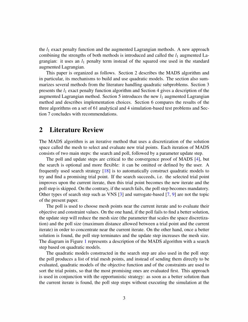
the l1 exact penalty function and the augmented Lagrangian methods. A new approachcombining the strengths of both methods is introduced and called the l1 augmented La-grangian: it uses an l1 penalty term instead of the squared one used in the standardaugmented Lagrangian.

This paper is organized as follows. Section 2 describes the MADS algorithm andin particular, its mechanisms to build and use quadratic models. The section also sum-marizes several methods from the literature handling quadratic subproblems. Section 3presents the l1 exact penalty function algorithm and Section 4 gives a description of theaugmented Lagrangian method. Section 5 introduces the new l1 augmented Lagrangianmethod and describes implementation choices. Section 6 compares the results of thethree algorithms on a set of 61 analytical and 4 simulation-based test problems and Sec-tion 7 concludes with recommendations.

2 Literature ReviewThe MADS algorithm is an iterative method that uses a discretization of the solutionspace called the mesh to select and evaluate new trial points. Each iteration of MADSconsists of two main steps: the search and poll, followed by a parameter update step.

The poll and update steps are critical to the convergence proof of MADS [4], butthe search is optional and more flexible: it can be omitted or defined by the user. Afrequently used search strategy [18] is to automatically construct quadratic models totry and find a promising trial point. If the search succeeds, i.e. the selected trial pointimproves upon the current iterate, then this trial point becomes the new iterate and thepoll step is skipped. On the contrary, if the search fails, the poll step becomes mandatory.Other types of search step such as VNS [3] and surrogate-based [7, 9] are not the topicof the present paper.

The poll is used to choose mesh points near the current iterate and to evaluate theirobjective and constraint values. On the one hand, if the poll fails to find a better solution,the update step will reduce the mesh size (the parameter that scales the space discretiza-tion) and the poll size (maximum distance allowed between a trial point and the currentiterate) in order to concentrate near the current iterate. On the other hand, once a bettersolution is found, the poll step terminates and the update step increases the mesh size.The diagram in Figure 1 represents a description of the MADS algorithm with a searchstep based on quadratic models.

The quadratic models constructed in the search step are also used in the poll step:the poll produces a list of trial mesh points, and instead of sending them directly to beevaluated, quadratic models of the objective function and of the constraints are used tosort the trial points, so that the most promising ones are evaluated first. This approachis used in conjunction with the opportunistic strategy: as soon as a better solution thanthe current iterate is found, the poll step stops without executing the simulation at the

3

Figure 1: An overview of the MADS algorithm with a search step based on quadraticmodels.

remaining trial points. Using quadratic models in both the search and poll steps greatlyimproves the MADS performance, as reported in [18].

At each iteration of MADS, a quadratic subproblem of the form (2) is constructed andsolved within the search step. The resulting solution is projected on the mesh to providea starting point that satisfies the convergence requirements of MADS. The subproblemis similar to those arising in trust-region methods called trust-region subproblems. Sincethe early eighties, many algorithms have been developed specifically to solve this kindof quadratic problems. The More & Sorenson algorithm (MS) [40] is one of the first al-gorithms used specifically for quadratic problems subject to an ellipsoidal constraint. Itis based on solving the optimality conditions via the Newton algorithm with backtrack-ing. The downside of this algorithm is that it uses Cholesky factorizations that becomeexpensive for large matrices. Later, the Generalized Lanczos Trust-Region algorithm(GLTR) [23] was implemented by using the MS algorithm on Krylov subspaces. How-ever, GLTR could not handle hard cases (see chapter 7 in [17]) of the trust-region sub-problems. The same principle is applied by the Sequential Subspace Method (SSM) [28]that creates four dimensional subspaces instead of using the Krylov subspaces. Even ifthe SSM algorithm handles the hard case of the trust-region subproblem, it still solvesquadratic problems over a sphere. The Gould-Robinson & Thorne algorithm [25] im-proved the MS algorithm by using some high dimensional polynomial approximationsthat allow the Newton method to converge in fewer iterations. Another algorithm, thattreats specifically quadratic problems over a convex quadratic constraint, is the Rendl

4

& Wolkowicz algorithm [21, 46] which rewrites the problem into an eigenvalue sub-problem that can be handled by the Newton method combined with Armijo-Goldsteinconditions. This algorithm is suitable for large-scale matrix problems.All the algorithms above are used for a quadratic objective over a unique constraint defin-ing the trust-region. In our case, Problem (2) is additionally constrained by m quadraticconstraints and, recently, one method was developed specifically for this kind of prob-lems using an extension of the Rendl & Wolkowicz algorithm [44]. Solving Problem (2)can also be done by nonlinear optimization tools such as exact penalty functions andaugmented Lagrangians. These two approaches are discussed further in the next twosections.

3 The l1 exact penalty function (l1EPF algorithm)The l1 exact penalty function starts by transforming Problem (2) into the followingbound-constrained problem:

minx∈X

f k(x)+ 1µ

m∑j=1

max(0,ckj(x))

subject to∥∥x− xk

∥∥∞≤ ∆k

(3)

where µ∈R+ is the penalty coefficient. This method was introduced by Zangwill in [52]and Pietrzykowski showed in [49] that, for µ sufficiently small, if the objective functionand the constraints are continuously differentiable, any local minimum of a nonlinearproblem would also be a minimizer of the l1 penalty function of that problem. In [35]and [52], it is shown that, in the convex case, there exists a threshold µ0 such as when µis smaller than µ0, a minimizer of the l1 penalty function would also be a minimizer ofthe nonlinear problem. Charalambous [10] generalizes this results under second orderconditions. In [11], Coleman and Conn explore optimality conditions of the l1 penaltyfunction. For our implementation, we concentrate on the approach provided by Colemanand Conn in [12, 13].

The objective function of (3) is not differentiable on the boundary of the domaindefined by ck(x)≤ 0. We introduce two subsets of indices at some point x ∈ X :

Aε ={

j ∈ J1,mK : |ckj(x)| ≤ ε

}and Vε =

{j ∈ J1,mK : ck

j(x) > ε

}. (4)

The set Aε contains the indices of ε-active constraints at x, and Vε regroups all the indicesof the ε-violated constraints at x. The remaining constraints whose indices are in { j ∈J1,mK : ck

j(x)≤−ε} (ε-satisfied) do not contribute locally to the objective function due tothe l1 term. Thus, for some neighborhood N (x)⊆ X of x, Problem (3) may be rewritten

5

as:

minx∈N (x)

pk(x,µ)+ 1µ ∑

j∈Aε

max(0,ckj(x))

subject to∥∥x− xk

∥∥∞≤ ∆k

(5)

where the penalty function pk(x,µ) := f k(x) + 1µ ∑

j∈Vε

max(0,ckj(x)) is differentiable at

x ∈ N (x). The second part of the objective function of (5) is not locally differentiable.In order to overcome this difficulty, we would like to find a descent direction h ∈ Rn

that would prevent any change in the ε-active constraints up to the second order whileminimizing the variation in the penalty function:

minh∈Rn

∇x pk(x,µ)>h+ 12h>∇xx pk(x,µ)h

subject to ∇ckj(x)>h+ 1

2h>∇2ckj(x)h = 0, j ∈ Aε.

(6)

Solving (6) approximately is detailed by Coleman and Conn in [13] and this processcircumvents the differentiability issues and explores a subspace where all the constraintsare far from being satisfied. We call h a range space minimization direction and it isused to reduce the penalty function while keeping the ε-active constraints constant. Thatis why each time x + h is close to a point x∗ that satisfies second-order sufficiency con-ditions, a null space minimization direction v is also needed and is used to improve theaction of the ε-active constraints:

φkAε

(x+h+ v) = 0 (7)

with φkAε

(x) = [ckj(x)] j∈Aε

the vector of ε-active constraints values at x. Using a Taylorexpansion up to the first order, the expression becomes:

φkAε

(x+h)+ JkAε

(x)>v≈ 0 (8)

with JkAε

(x) = [∇ckj(x)] j∈Aε

the matrix of ε-active constraints gradients. Then v can becomputed by solving the linear system:

JkAε

(x)>v =−φkAε

(x+h). (9)

When v is computed, the iterate is updated along the direction h + v with a stepsizeof 1 only if it presents a sufficient decrease. Algorithm 1 summarizes the inner iterationof the l1EPF algorithm.

Algorithm 1 provides an overview of the methodology used to select a descent di-rection (See [13] for the complete description). A line-search algorithm tailored forpiecewise differentiable functions is described in [13]. The overall algorithm tries sim-ply, at each iteration, to find a minimizer of the penalty function for a fixed value ofµ (Algorithm 1) and then proceeds to reduce µ if the selected minimizer is infeasible

6

Algorithm 1: l1EPF algorithm (inner iteration) [13]1: Initialization of ε, x, Aε and Vε

2: If the stopping criteria are met: STOPOtherwise go to 3

3: Compute h (by approximately solving (6))4: if x is close to a point satisfying the 2nd order sufficiency conditions then5: Compute v (by solving (9))6: if x+h+ v decreases p sufficiently then7: x← x+h+ v8: else9: Update ε, Aε and Vε

10: Compute h (by approximately solving (6))11: Compute the step size β (Line-search algorithm)12: x← x+βh13: end if14: else15: Compute the step size β (Line-search algorithm)16: x← x+βh17: end if18: Go to 2.

for (2) in order to put more weight on the constraints. Algorithm 2 describes the outeriteration of the l1EPF method.

Algorithm 2: l1EPF algorithm (outer iteration) [13]1: Initialization of µ and x2: while x is not feasible do3: Minimize p to find new iterate x (Algorithm 1)4: Update: µ = µ/105: end while

4 Augmented Lagrangian (AugLag)The augmented Lagrangian method was introduced by Powell [45] and Hestenes [30] inthe late sixties. Since that time, the method was widely studied, improved and supportedby convergence analyses [27, 43] and different versions of the algorithm were imple-mented. A well-known implementation is the LANCELOT package [14, 16]. Whenusing slack variables in the implementation, it is possible to exploit the structure of

7

these variables to increase the efficiency of the algorithm [15, 20]. An augmented La-grangian for constrained blackbox problems is designed in [26]. The paper [8] introducesa derivative-free trust-region algorithm (DFTR) that uses the augmented Lagrangian ap-proach to solve quadratically constrained quadratic subproblems and provides a methodto update the trust-region radius. In the present work, we follow the approach describedin [2] which is similar to the LANCELOT implementation.

First, slack variables s ∈ Rm are added to Problem (2):

minx∈X , s∈Rm

f k(x)

subject to ckj(x)+ s j = 0, j ∈ J1,mK∥∥x− xk

∥∥∞≤ ∆k,

s j ≥ 0, j ∈ J1,mK

(10)

and the bound constrained augmented Lagrangian is defined as follows:

minx∈X , s∈Rm

Lka(x,s,λ,µ) = f k(x)−

m∑j=1

λ j(ckj(x)+ s j)+ 1

2µ

m∑j=1

(ckj(x)+ s j)2

subject to∥∥x− xk

∥∥∞

≤ ∆k,s j ≥ 0, j ∈ J1,mK

(11)

where λ ∈ Rm and µ ∈ R+. The augmented Lagrangian algorithm solves (11) at eachiteration l of the outer algorithm for fixed values λl and µl to compute the next iterate(xl+1,sl+1). The index l counts the outer iterations of the augmented Lagrangian methodwhile the index k characterizes the subproblem (2). The outer iteration proceeds to up-date one of the parameters λl or µl: when all the constraints values are below a giventolerance value, ηl , the iterate is judged locally feasible and the algorithm proceeds toupdate the multipliers λl . In the other case, the penalty parameter µ is reduced in order togive more importance to the constraints and try to satisfy them on the next iteration. Al-gorithm 3 gives an overview of the outer iteration of the augmented Lagrangian method:

To compute the next iterate in step 3 of Algorithm 3, a quadratic model is used toapproximate (11) at each iteration l of the outer loop:

mindx∈Rn, ds∈Rm

∇xLka(xl,sl,λl,µl)>dx + 1

2dx>∇xxLka(xl,sl,λl,µl)dx+

∇sLka(xl,sl,λl,µl)>ds + 1

2ds>∇ssLka(xl,sl,λl,µl)ds

subject to∥∥xl +dx− xk

∥∥∞≤ ∆k,

sl +ds ≥ 0,‖dx‖

∞≤ δl,

‖ds‖∞≤ δl

(12)

with δl the trust-region of the model. To simplify, let d ∈ Rn+m be the concatenation ofdx and ds (d> = [dx>ds>]) and y ∈ Rn+m the concatenation of x and s (y> = [x>s>]).

8

Algorithm 3: Augmented Lagrangian to solve Problem (10): outer iteration [2]

1: Initializations: l = 0, λl, µl, ηl, xl, sl

2: If the stopping criteria are met: STOPOtherwise go to 3

3: Compute the next iterate: (xl+1,sl+1) by solving (11)for fixed values of λl and µl (Algorithm 5)

4: if∥∥c(xl+1)+ sl+1

∥∥∞≤ ηl then

5: λl+1← λl− 1µl (ck(xl)+ sl)

6: ηl+1← ηl(µl)0.9

7: else8: µl+1← µl

10

9: ηl+1← (µl+1)0.1

1010: end if11: l← l +112: Go to 2.

Since the constraints of (12) form a box B , it is possible to define lower and upperbounds l ∈ Rn+m and u ∈ Rn+m and define the feasible set:

B = {d ∈ Rn+m : l ≤ d ≤ u}. (13)

Problem (12) is rewritten as:

mind∈B

∇yLka(yl,λl,µl)>d + 1

2d>∇yyLka(yl,λl,µl)d. (14)

Solving (14) relies on an iterative method developed by More & Toraldo to treatbox constrained quadratic problems (see [2, 41]). We chose this approach due to somepreliminary results on unconstrained problems that favored this trust-region method overthe line-search method used in the previous section. The More & Toraldo algorithmmanipulates the active-set A(d) = {i∈ J1,n+mK : di = `i or di = ui} to look for a descentdirection p that would be used to update its current iterate d via a line-search. In the firststage of the algorithm, a promising face containing d is selected via a projected gradientmethod. A face of B is defined as a set of vectors for which active-set A(d) coordinatescoincide with d:

F = {w ∈ B : wi = di for i ∈ A(d)}. (15)

The second part of the More & Toraldo method concentrates on finding a descentdirection p on the selected face with a conjugate gradient algorithm and update d. Algo-rithm 4 summarizes the More & Toraldo method to compute the solution d to (14):

9

Algorithm 4: algorithm PG/CG [41]1: while no solution d is found do2: Use the projected gradient (PG) method to select a promising face of the

feasible set B .3: Use the conjugate gradient (CG) method to explore the selected face and

find a descent direction p.4: Use a projected line-search alongside p to choose the next iterate d.5: end while

Once a direction d is computed, the inner iteration of the augmented Lagrangianmethod uses a typical trust-region approach: the ratio r (defined in Step 4 of Algorithm 5)determines whether the model fits the augmented Lagrangian function well. If the ratiois close to 1, the model fits the function well and, in that case, the trust-region radiusmust increase. On the contrary, if the ratio is negative or close to zero, the trust-regionmust be reduced. The ratio r also allows one to decide if the iterate x gets updated ornot. Algorithm 5 describes the inner iteration of the augmented Lagrangian method.

Algorithm 5: Augmented Lagrangian: inner iteration [2]1: Initializations: 0 < ε1 ≤ ε2 < 1, d and 0 < γ1 < 1 < γ22: If the stopping criteria are met: STOP

Otherwise go to 33: Solve (14) to find d

4: Compute the ratio : r =Lk

a(yl +d,λl,µl)−Lka(yl,λl,µl)

∇Lka(yl,λl,µl)>d + 1

2d>∇2Lka(yl,λl,µl)d

5: if r ≥ ε1 then6: xl ← xl +d7: if r ≥ ε2 then8: δ← γ2 max(‖d‖

∞,δ)

9: end if10: else11: δ← γ1 ‖d‖∞

12: end if13: Go to 2.

5 Augmented Lagrangian with l1 penalty term (l1AugLag)The present section proposes a new method that combines the algorithms from the previ-ous two sections. Since the constraints in Problem (2) are quadratic rather than general

10

nonlinear, the augmented Lagrangian loses the quadratic structure of the subproblemdue to the squared penalty term. The idea is to replace this part with a l1 penalty termin order to get a piecewise quadratic function. We define the l1 augmented Lagrangianproblem in the following manner:

minx∈X

f k(x)−m∑j=1

λ jckj(x)+ 1

µ

m∑j=1

max{0,ckj(x)}

subject to∥∥x− xk

∥∥∞≤ ∆k.

(16)

By using the same definition as in Equation (4) of ε-active and ε-violated sets fora point x = xl (at iteration l of the outer approximation), it is possible to restrict theanalysis of Problem (16) in a neighborhood N (xl)⊆ X of xl (same approach as in (5)):

minx∈N (xl)

Dk(x,λ,µ)+ 1µ ∑

j∈Aε

max{0,ckj(x)}

subject to∥∥x− xk

∥∥∞≤ ∆k

(17)

where Dk(x,λ,µ) = f k(x)−m∑j=1

λ jckj(x) + 1

µ ∑j∈Vε

ckj(x) is differentiable, but the second

term involving Aε is not. This is similar to the l1 exact penalty approach: At eachiteration l, we need to handle the differentiability issues by concentrating on computinga direction that minimizes the variation in the l1 augmented Lagrangian expression andkeeps the ε-active constraints from varying for fixed values of λ and µ:

minh∈Rn

∇xDk(xl,λl,µl)>h+ 12h>∇xxDk(xl,λl,µl)h

subject to ∇ckj(x

l)>h+ 12h>∇2ck

j(xl)h = 0, j ∈ Aε.

(18)

To further satisfy the ε-active constraints, we can use (9) to compute a null spaceminimization direction v. Algorithm 1 still applies: we just have to compute the rangespace minimization direction h in Steps 3 and 10 by solving (18) instead. The outer it-eration algorithm has to update either λ or µ which is why the l1 exact penalty approachalone is not preferred. Instead, we can use a method similar to the outer iteration algo-rithm of the augmented Lagrangian: we can keep updating the penalty parameter µ inthe same way, but the λ update needs some adjustment. We can determine how to updateλ by using the optimality test:

∇kxL(xl,λl) = 0 (19)

with L(x,λ) = f (x)−m∑j=1

λ jckj(x), the Lagrangian of Problem (2). So, at iteration l, if

xl+1 is a minimizer of (17), then there exists a vector λ for which:

∇ f k(xl+1)−m

∑j=1

λ j∇ckj(x

l+1)+1µ ∑

j∈Vε

∇ckj(x

l+1)− ∑j∈Aε

λ j∇ckj(x

l+1) = 0. (20)

11

If we define λl+1 to be:

λl+1 =

λl

j + λ j, if j ∈ Aε

λlj−

1µ , if j ∈Vε

λlj, if j 6∈ Aε∪Vε

(21)

then the optimality test (19) becomes:

∇xL(xl+1,λl+1) = ∇ f k(xl+1)−m∑j=1

λl+1j ∇ck

j(xl+1)

= ∇ f k(xl+1)− ∑j 6∈Aε∪Vε

λlj∇ck

j(xl+1)

− ∑j∈Vε

(λlj−

1µ)∇ck

j(xl+1)− ∑

j∈Aε

(λlj + λ j)∇ck

j(xl+1)

= ∇ f k(xl+1)−m∑j=1

λ j∇ckj(x

l+1)+ 1µ ∑

j∈Vε

∇ckj(x

l+1)

− ∑j∈Aε

λ j∇ckj(x

l+1)

= 0

(22)

which confirms our update method of λ. The only remaining issue is how to compute λ.Equation (20) is rewritten as:

∑j∈Aε

λ j∇ckj(x

l+1) = ∇ f k(xl+1)−m

∑j=1

λ j∇ckj(x

l+1)+1µ ∑

j∈Vε

∇ckj(x

l+1). (23)

By using matrix notations, Equation (23) becomes:

JkAε

λ = ∇Dk(xl+1,λl+1,µl+1) (24)

where JkAε

is the matrix of ε-active constraint gradients defined in Section 3. By using aQR decomposition, there exists an orthogonal matrix Q and an upper triangular matrixU such that:

JkAε

= QR = [Q1 Q2][

U0

]= Q1U (25)

where the number of columns of Q1 is the same as the number of rows of U and corre-sponds to the number of ε-active constraints near x. We can use this to transform (24)into:

U λ = Q>1 ∇Dk(xl+1,λl+1,µl+1). (26)

It is now easy to get λ by using a backward substitution algorithm. Algorithm 6 displaysthe outer iteration of the l1AUGLAG method:

12

Algorithm 6: l1 augmented Lagrangian: outer iteration

1: Initializations: l = 0, λl, µl, ηl, xl, sl

2: If the stopping criteria are met: STOPOtherwise go to 3

3: Compute the next iterate: xl+1 by minimizing (17)for fixed values of λl and µl .

4: if ckj(x

l+1)≤ ηl for all j ∈Vε then

5: λl+1←

λl

j + λ j, j ∈ Aε

λlj−

1µ , j ∈Vε

λlj, j 6∈ Aε & j 6∈Vε

6: ηl+1← ηl(µl)0.9

7: else8: µl+1← µl

10

9: ηl+1← (µl+1)0.1

1010: end if11: l← l +112: Go to 2.

6 Computational resultsIn this section, we introduce three sets of test problems for the comparison between fivevariants of NOMAD: each version uses a different approach to solve Subproblem (2).The results of this comparison are detailed in Subsections 6.2, 6.3 and 6.4.

6.1 Test problemsWe use three sets of optimization problems of the form (1): the first set is composed of42 unconstrained problems, the second consists of 19 constrained problems and the thirdcontains 4 simulation-based applications: two MDO problems called AIRCRAFT RAN-GE and SIMPLIFIED WING, a structural engineering design problem of a welded beamcalled WELDED and a blackbox optimization problem (LOCKWOOD) which mini-mizes the cost of managing wells in the Lockwood Solvent Groundwater Plume Site(Montana) that prevents the contamination of the Yellowstone River. Table 1 regroupsthe name, dimension and number of constraints of the 65 test problems.

We implemented the three methods of Sections 3, 4 and 5 into the NOMAD pack-age [34] (www.gerad.ca/nomad) and compare five algorithmic variants. The first vari-ant is denoted MADS and uses the current version of NOMAD (version 3.7) to solveSubproblem (2). The three variants l1EPF, AUGLAG and l1AUGLAG respectively use thel1 exact penalty function, the augmented Lagrangian and the l1 augmented Lagrangian

13

Table 1: Description of the test problems.Name n m Source Name n m Source Name n m Source

Unconstrained ConstrainedACKLEY 10 0 [29] POWELLSG 12 0 [24] CRESCENT10 10 2 [5]

ARWHEAD 10 0 [24] POWELLSG 20 0 [24] DISK10 10 1 [5]ARWHEAD 20 0 [24] RADAR 7 0 [39] G1 13 9 [38]BDQRTIC 10 0 [24] RANA 2 0 [32] G2 10 2 [38]BDQRTIC 20 0 [24] RASTRIGIN 2 0 [29] G2 20 2 [38]BIGGS6 6 0 [24] RHEOLOGY 3 0 [6] G4 5 6 [38]BRANIN 2 0 [29] ROSENBROCK 2 0 [32] G6 2 2 [38]

BROWNAL 10 0 [24] SCHWEFEL 2 0 [47] G7 10 8 [38]BROWNAL 20 0 [24] SHOR 5 0 [36] G8 2 2 [38]

DIFF2 2 0 [18] SROSENBR 10 0 [24] G9 7 4 [38]ELATTAR 6 0 [36] SROSENBR 20 0 [24] G10 8 6 [38]

EVD61 6 0 [36] TREFETHEN 2 0 [32] HS44 4 6 [31]FILTER 9 0 [36] TRIDIA 10 0 [24] HS64 3 1 [31]

GRIEWANK 2 0 [29] TRIDIA 20 0 [24] HS93 6 2 [31]GRIEWANK 10 0 [29] VARDIM 10 0 [24] HS108 9 13 [31]

HS78 5 0 [36] VARDIM 20 0 [24] HS114 9 6 [36]OSBORNE2 11 0 [36] WATSON 12 0 [32] MAD6 5 7 [36]

PBC1 5 0 [36] WONG1 7 0 [36] PENTAGON 6 15 [36]PENALTY1 10 0 [24] WONG2 10 0 [36] SNAKE 2 2 [5]PENALTY1 20 0 [24] WOODS 12 0 [24]

POLAK2 10 0 [36] WOODS 20 0 [24]Simulation-based MDO applications

AIRCRAFT RANGE 10 10 [1, 48] SIMPLIFIED WING 7 3 [50] WELDED 4 6 [22]LOCKWOOD 6 4 [33, 37]

to treat (2). Finally, the last variant uses the IPOPT package [51] which is software fornonlinear optimization. The tests were conducted on a Linux machine with an Intel(R)Core(TM) i7-2600 (3.40 GHz) processor.

To compare these five methods, we rely on the More & Wild performance and dataprofiles [42] by considering the following formula as the main convergence test:

f (x f )− f (x)≥ (1− τ)( f (x f )− f ∗) (27)

where τ is the convergence precision, f ∗ is the best solution found by all solvers for aspecific problem and a given budget (of either evaluations or time) and x f is the first fea-sible point of the problem found by any solver. If a solver cannot find a feasible solution,the convergence test will always fail which will favor all the solvers that find at least onefeasible point. Performance profiles show the ratio of solved problems according to aperformance ratio α defined as the upper bound of the number of evaluations neededto satisfy the convergence test. These profiles allow one to compare the relative perfor-mances of the algorithms. Data profiles, on the other hand, indicate which algorithms isbest for a fixed number of function evaluations: they show the ratio of solved problemsto groups of n+1 function evaluations.

14

6.2 Unconstrained test setProblems of the first test set are unconstrained. It implies that penalty parameters andLagrange multipliers are not necessary and our methods reduce to their inner iterations:the l1EPF and l1AUGLAG become an iterative line-search method that uses matrix de-compositions to select the descent direction, while the AUGLAG method solves a trust-region subproblem with a combination of projected and conjugate gradient methods.Figure 2(a) regroups performance profiles for the unconstrained set with τ = 10−3. Itis difficult to set a winner apart from this graph: for example, IPOPT starts slowly, butemerges on top for a performance ratio α = 3. Figures 2(b) and 2(c) represent perfor-mance and data profiles for the first set of problems with a precision τ = 10−7. AUGLAGclearly outperforms the other methods in this case.

Figure 2(d) regroups time data profiles: they show the ratio of solved problems withprecision τ = 10−7 for a given time budget. This figure takes into account the effortdeployed to solve the quadratic subproblems and confirms the superiority of AUGLAG forunconstrained optimization. We conclude that a trust-region is preferable to a line-searchmethod to solve the augmented Lagrangian subproblem in the absence of constraints inProblem (2).

Even if the l1EPF and l1AUGLAG reduce to the same inner iteration, we can see thatthere are differences in the profiles because these algorithms choose different startingpoints for the subproblem. This implementation choice was done after several prelim-inary tests on constrained problems and was kept for the unconstrained case. Still, thevariations between l1EPF and l1AUGLAG are small and the two methods seem equiva-lent.

6.3 Constrained test setThe problems of the second set are constrained. Figure 3 shows performance and dataprofiles for precisions τ = 10−3 and τ = 10−7. For this set of problems, all the new meth-ods outperform MADS, especially l1AUGLAG which gives the best results and solvesalmost 95% of the problems while the MADS-based NOMAD solves only 75% whenτ = 10−7 as illustrated in the performance profiles of Figure 3(a).

Figure 3(d) represents time data profiles for the second set of test problems: usingIPOPT to solve subproblems seems to be efficient timewise, but still, the figure confirmsthat l1AUGLAG is the best approach for the constrained case.

6.4 Simulation-based applicationsFor the last set, we create 50 different instances for each of the four applications: fora given problem, a Latin hypercube sampling generates 50 starting points and each ofthese instances is solved by the five variants of NOMAD. Some of these starting points

15

(a) Performance profiles for τ = 10−3. (b) Performance profiles for τ = 10−7.

(c) Data profiles for τ = 10−7. (d) Time data profiles for τ = 10−7.

Figure 2: Performance and data profiles on the unconstrained test set.

are feasible, others are not. These simulated-based problems tend to be timewise compu-tationally expensive: the 750 tests of AIRCRAFT RANGE, SIMPLIFIED WING andWELDED ran for over five days and the 250 runs of LOCKWOOD, took almost twoweeks of execution time.For each application, we draw data and performance profiles to compare the differentmethods (we consider that all the instances are different problems). It is importantto carefully select an appropriate value of the precision parameter τ for each problemsince, on one hand, if τ is too small, the profiles tends to pile up with a small proportionof problems solved. On the other hand, if τ is too large, the curves converge to 100%problem solved quickly. For clarity, we chose values of τ as the power of 10 that spreads

16

(a) Performance profiles for τ = 10−3. (b) Performance profiles for τ = 10−7.

(c) Data profiles for τ = 10−7. (d) Time data profiles for τ = 10−7.

Figure 3: Performance and data profiles on the constrained test set.

out as much as possible the profiles.In Figures 4 and 5, we can immediately see that l1AUGLAG is the best approach for

the AIRCRAFT RANGE and LOCKWOOD problems. But, while l1EPF and IPOPTseem to give good results on the AIRCRAFT RANGE application (they are even over-lapping l1AUGLAG for α ≤ 1.3), AUGLAG and MADS are more efficient on the LOCK-WOOD problem.

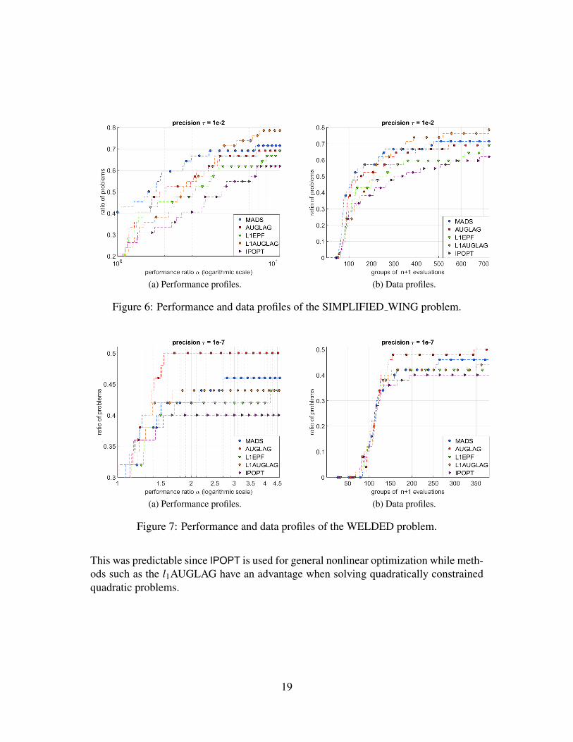
In Figure 6, MADS shows some good results when α≤ 4.5 and the budget is limitedto 300 (n + 1) evaluations. When we allow more evaluation budget, l1AUGLAG canalmost reach 80% of problems solved.

In Figure 7, the AUGLAG approach outperforms the rest of the algorithms with

17

(a) Performance profiles. (b) Data profiles.

Figure 4: Performance and data profiles of the AIRCRAFT RANGE problem.

(a) Performance profiles. (b) Data profiles.

Figure 5: Performance and data profiles of the LOCKWOOD problem.

IPOPT coming last again.These profiles suggest that IPOPT should be discarded as a replacement for MADS

in solving the quadratic subproblem. To recommend an alternative for MADS amongthe three proposed methods, we build performance and data profiles with τ = 10−2 andτ = 10−5 for the combined 200 instances of the four simulation-based applications.

In Figure 8, l1AUGLAG seems to be the clear winner. As suspected, IPOPT is nota viable option to solve the subproblem, while the three remaining approaches, MADS,l1EPF and AUGLAG, are competitive with each other on the simulation-based problems.

18

(a) Performance profiles. (b) Data profiles.

Figure 6: Performance and data profiles of the SIMPLIFIED WING problem.

(a) Performance profiles. (b) Data profiles.

Figure 7: Performance and data profiles of the WELDED problem.

This was predictable since IPOPT is used for general nonlinear optimization while meth-ods such as the l1AUGLAG have an advantage when solving quadratically constrainedquadratic problems.

19

(a) Performance profiles. (b) Data profiles.

(c) Performance profiles. (d) Data profiles.

Figure 8: Performance and data profiles for all 200 instances of the simulation-basedapplications.

7 DiscussionThis work details the implementation of two existing nonlinear optimization methods(l1EPF and AUGLAG) and the development of a new algorithm called the l1 augmentedLagrangian method (l1AUGLAG). These methods are used within a derivative-free opti-mization framework to solve quadratically constrained quadratic subproblems that arisewhen using quadratic models of the objective function and of the constraints. It wouldbe possible to use the implemented methods within algorithms that rely on treating sub-problems to solve general nonlinear problems with derivatives. Another avenue would

20

be to use the augmented Lagrangian method to transform a DFO problem with generalequality constraints into an unconstrained problem that MADS can deal with.

This paper shows that using a dedicated algorithm to solve quadratic subproblemsimproves the overall performance of MADS with quadratic models. The results showthat, in the unconstrained case, using a trust-region approach (inner iteration of the aug-mented Lagrangian) yields better result than line-search method (which is the case forboth the l1 exact penalty function and the l1 augmented Lagrangian).

The l1AUGLAG approach gives the best results in the constrained case as, we be-lieve, it combines the strengths of both AUGLAG and l1EPF methods: the Lagrangemultipliers terms improve the computation performances and the l1 penalty term allowsProblem (16) to have a piecewise quadratic structure.

In all cases, there is at least one method that improves over MADS in regards of bothresults and time and this is the main goal of the paper. The computational results showalso that at least one of the three suggested methods is performing better than IPOPTwhich validates the choice of implementing a dedicated method for NOMAD.

We conclude with recommendations for the NOMAD software package. For solv-ing quadratic subproblems in the search step, NOMAD should use the More & Toraldoaugmented Lagrangian algorithm in the unconstrained case and the l1 augmented La-grangian method for constrained problems.

References[1] J.S. Agte, J. Sobieszczanski-Sobieski, and R.R.J. Sandusky. Supersonic business

jet design through bilevel integrated system synthesis. In Proceedings of the WorldAviation Conference, volume SAE Paper No. 1999-01-5622, San Francisco, CA,1999. MCB University Press, Bradford, UK.

[2] S. Arreckx, A. Lambe, J.R.R.A. Martins, and D. Orban. A matrix-free augmentedlagrangian algorithm with application to large-scale structural design optimization.Optimization and Engineering, 17(2):359–384, 2016.

[3] C. Audet, V. Bechard, and S. Le Digabel. Nonsmooth optimization through meshadaptive direct search and variable neighborhood search. Journal of Global Opti-mization, 41(2):299–318, 2008.

[4] C. Audet and J.E. Dennis, Jr. Mesh adaptive direct search algorithms for con-strained optimization. SIAM Journal on Optimization, 17(1):188–217, 2006.

[5] C. Audet and J.E. Dennis, Jr. A Progressive Barrier for Derivative-Free NonlinearProgramming. SIAM Journal on Optimization, 20(1):445–472, 2009.

[6] C. Audet and W. Hare. Derivative-Free and Blackbox Optimization, In preparation.

21

[7] C. Audet, M. Kokkolaras, S. Le Digabel, and B. Talgorn. Order-based error formanaging ensembles of surrogates in derivative-free optimization. Technical Re-port G-2016-36, Les cahiers du GERAD, 2016.

[8] C. Audet, S. Le Digabel, and M. Peyrega. A derivative-free trust-region augmentedLagrangian algorithm. Technical Report G-2016-53, Les cahiers du GERAD, 2016.

[9] A.J. Booker, J.E. Dennis, Jr., P.D. Frank, D.B. Serafini, V. Torczon, and M.W.Trosset. A Rigorous Framework for Optimization of Expensive Functions by Sur-rogates. Structural and Multidisciplinary Optimization, 17(1):1–13, 1999.

[10] C. Charalambous. A lower bound for the controlling parameters of the exactpenalty functions. Mathematical programming, 15(1):278–290, 1978.

[11] T.F. Coleman and A.R. Conn. Second-order conditions for an exact penalty func-tion. Mathematical Programming, 19(1):178–185, 1980.

[12] T.F. Coleman and A.R. Conn. Nonlinear programming via an exact penalty func-tion: Asymptotic analysis. Mathematical programming, 24(1):123–136, 1982.

[13] T.F. Coleman and A.R. Conn. Nonlinear programming via an exact penalty func-tion: Global analysis. Mathematical Programming, 24(1):137–161, 1982.

[14] A.R. Conn, N.I.M. Gould, and Ph.L. Toint. LANCELOT: a Fortran package forlarge-scale nonlinear optimization (release A). Springer, New-York, 1992.

[15] A.R. Conn, N.I.M. Gould, and Ph.L. Toint. A note on exploiting structure whenusing slack variables. Mathematical Programming, 67(1):89–97, 1994.

[16] A.R. Conn, N.I.M. Gould, and Ph.L. Toint. Numerical experiments with theLANCELOT package (release A) for large-scale nonlinear optimization. Math-ematical Programming, 73(1):73–110, 1996.

[17] A.R. Conn, N.I.M. Gould, and Ph.L. Toint. Trust region methods. SIAM, 2000.

[18] A.R. Conn and S. Le Digabel. Use of quadratic models with mesh-adaptive directsearch for constrained black box optimization. Optimization Methods and Soft-ware, 28(1):139–158, 2013.

[19] A.R. Conn, K. Scheinberg, and L.N. Vicente. Introduction to Derivative-Free Op-timization. MOS-SIAM Series on Optimization. SIAM, Philadelphia, 2009.

[20] A.R. Conn, L.N. Vicente, and C. Visweswariah. Two-step algorithms for non-linear optimization with structured applications. SIAM Journal on Optimization,9(4):924–947, 1999.

22

[21] C. Fortin and H. Wolkowicz. The trust region subproblem and semidefinite pro-gramming. Optimization Methods and Software, 19(1):41–67, 2004.

[22] H. Garg. Solving structural engineering design optimization problems using an ar-tificial bee colony algorithm. Journal of Industrial and Management Optimization,10(3):777–794, 2014.

[23] N.I.M. Gould, S. Lucidi, and Ph.L. Toint. Solving the trust-region subproblemusing the Lanczos method. SIAM Journal on Optimization, 9(2):504–525, 1999.

[24] N.I.M. Gould, D. Orban, and Ph.L. Toint. CUTEr (and SifDec): A constrained andunconstrained testing environment, revisited. ACM Transactions on MathematicalSoftware, 29(4):373–394, 2003.

[25] N.I.M. Gould, D.P. Robinson, and H.S. Thorne. On solving trust-region and otherregularised subproblems in optimization. Mathematical Programming Computa-tion, 2(1):21–57, 2010.

[26] R.B. Gramacy, G.A. Gray, S. Le Digabel, H.K.H. Lee, P. Ranjan, G. Wells, andS.M. Wild. Modeling an Augmented Lagrangian for Blackbox Constrained Opti-mization. Technometrics, 58(1):1–11, 2016.

[27] I. Griva, S.G. Nash, and A. Sofer. Linear and Nonlinear Optimization. Society forIndustrial and Applied Mathematics, 2009.

[28] W.W. Hager. Minimizing a quadratic over a sphere. SIAM Journal on Optimization,12(1):188–208, 2001.

[29] A.-R. Hedar. Global optimization test problems. http://www-optima.amp.i.kyoto-u.ac.jp/member/student/hedar/Hedar_files/TestGO.htm.

[30] M.R. Hestenes. Multiplier and gradient methods. Journal of Optimization Theoryand Applications, 4(5):303–320, 1969.

[31] W. Hock and K. Schittkowski. Test Examples for Nonlinear Programming Codes,volume 187 of Lecture Notes in Economics and Mathematical Systems. Springer,Berlin, Germany, 1981.

[32] M. Jamil and X.-S. Yang. A literature survey of benchmark functions for globaloptimisation problems. International Journal of Mathematical Modelling and Nu-merical Optimisation, 4(2):150–194, 2013.

[33] A. Kannan and S.M. Wild. Benefits of Deeper Analysis in Simulation-basedGroundwater Optimization Problems. In Proceedings of the XIX InternationalConference on Computational Methods in Water Resources (CMWR 2012), June2012.

23

[34] S. Le Digabel. Algorithm 909: NOMAD: Nonlinear Optimization with the MADSalgorithm. ACM Transactions on Mathematical Software, 37(4):44:1–44:15, 2011.

[35] D.G. Luenberger. Control problems with kinks. IEEE Transactions on AutomaticControl, 15(5):570–575, 1970.

[36] L. Luksan and J. Vlcek. Test problems for nonsmooth unconstrained and linearlyconstrained optimization. Technical Report V-798, ICS AS CR, 2000.

[37] L.S. Matott, A.J. Rabideau, and J.R. Craig. Pump-and-treat optimization usinganalytic element method flow models. Advances in Water Resources, 29(5):760–775, 2006.

[38] Z. Michalewicz and M. Schoenauer. Evolutionary algorithms for constrained pa-rameter optimization problems. Evolutionary computation, 4(1):1–32, 1996.

[39] N. Mladenovic, J. Petrovic, V. Kovacevic-Vujcic, and M. Cangalovic. Solvingspread spectrum radar polyphase code design problem by tabu search and variableneighbourhood search. European Journal of Operational Research, 151(2):389–399, 2003.

[40] J.J. More and D.C. Sorensen. Computing a trust region step. SIAM Journal onScientific Computing, 4(3):553–572, 1983.

[41] J.J. More and G. Toraldo. On the solution of large quadratic programming problemswith bound constraints. SIAM Journal on Optimization, 1(1):93–113, 1991.

[42] J.J. More and S.M. Wild. Benchmarking derivative-free optimization algorithms.SIAM Journal on Optimization, 20(1):172–191, 2009.

[43] J. Nocedal and S.J. Wright. Numerical Optimization. Springer Series in OperationsResearch. Springer, New York, 1999.

[44] T.K. Pong and H. Wolkowicz. The generalized trust region subproblem. Compu-tational Optimization and Applications, 58(2):273–322, 2014.

[45] M.J.D. Powell. A method for nonlinear constraints in minimization problems.In R. Fletcher, editor, Optimization, pages 283–298. Academic Press, New York,1969.

[46] F. Rendl and H. Wolkowicz. A semidefinite framework for trust region subprob-lems with applications to large scale minimization. Mathematical Programming,77(1):273–299, 1997.

[47] H.-P. Schwefel. Numerical Optimization of Computer Models. John Wiley & Sons,Inc., New York, NY, USA, 1981.

24

[48] J. Sobieszczanski-Sobieski, J.S. Agte, and R.R. Sandusky, Jr. Bi-Level IntegratedSystem Synthesis (BLISS). Technical Report NASA/TM-1998-208715, NASA,Langley Research Center, 1998.

[49] T. Pietrzykowski. An exact potential method for constrained maxima. SIAM Jour-nal on numerical analysis, 6(2):299–304, 1969.

[50] C. Tribes, J.-F. Dube, and J.-Y. Trepanier. Decomposition of multidisciplinaryoptimization problems: formulations and application to a simplified wing design.Engineering Optimization, 37(8):775–796, 2005.

[51] A. Wachter and L. T. Biegler. On the implementation of a primal-dual interior pointfilter line search algorithm for large-scale nonlinear programming. MathematicalProgramming, 106(1):25–57, 2006.

[52] W.I. Zangwill. Non-linear programming via penalty functions. Management sci-ence, 13(5):344–358, 1967.

25