efficient techniques for depth video compression using...
TRANSCRIPT

1
Efficient Techniques for Depth Video Compression
Using Weighted Mode FilteringViet-Anh Nguyen, Dongbo Min, Member, IEEE, and Minh N. Do, Senior Member, IEEE
Abstract— This paper proposes efficient techniques to com-press a depth video by taking into account coding artifacts, spatialresolution, and dynamic range of the depth data. Due to abruptsignal changes on object boundaries, a depth video compressedby conventional video coding standards often introduces seriouscoding artifacts over object boundaries, which severely affect thequality of a synthesized view. We suppress the coding artifactsby proposing an efficient post-processing method based on aweighted mode filtering and utilizing it as an in-loop filter.In addition, the proposed filter is also tailored to reconstructefficiently the depth video from the reduced spatial resolution andthe low dynamic range. The down/upsampling coding approachesfor the spatial resolution and the dynamic range are used togetherwith the proposed filter in order to further reduce the bit rate.We verify the proposed techniques by applying to an efficientcompression of multiview-plus-depth data, which has emergedas an efficient data representation for 3D video. Experimentalresults show that the proposed techniques significantly reducethe bit rate while achieving a better quality of the synthesizedview in terms of both objective and subjective measures.
Index Terms— Weighted mode filtering, depthdown/upsampling, depth dynamic range, depth coding, 3Dvideo
I. INTRODUCTION
With the recent development of 3D multimedia/display tech-
nologies and the increasing demand for realistic multimedia,
3D video has gained more attentions as one of the most
dominant video formats with a variety of applications such as
3-dimensional TV (3DTV) or freeview point TV (FTV). 3DTV
aims to provide users with 3D depth perception by rendering
two (or more) views on stereoscopic (or auto-stereoscopic)
3D display. FTV can give users the freedom of selecting a
viewpoint, different from conventional TV where the view-
point is determined by an acquisition camera. 3D freeview
video can also be provided by synthesizing multiple views at
the selected viewpoint according to a user preference [1]. For
successful development of 3D video systems, many technical
issues should be resolved, e.g. capturing and analyzing the
stereo or multiview images, compressing and transmitting the
data, and rendering multiple images on various 3D displays.
The main challenging issues of 3DTV and FTV are depth
estimation, virtual view synthesis, and 3D video coding. The
This study is supported by the research grant for the Human Sixth SenseProgramme at the Advanced Digital Sciences Center from Singapore’s Agencyfor Science, Technology and Research (A*STAR).
V.-A. Nguyen and D. Min are with the Advanced Digital Sciences Center,Singapore 138632 (email: [email protected]; [email protected]).
M. N. Do is with the University of Illinois at Urbana-Champaign, Urbana,IL 61820-5711 USA (email: [email protected]).
depth maps are used to synthesize the virtual view at the
receiver side, so accurate depth maps should be estimated in
an efficient manner for ensuring a seamless view synthesis.
Since the performance of 3DTV and FTV heavily depends
on the number of multiple views, virtual view synthesis is an
important technique in 3D video systems as well. In other
words, synthesizing virtual view with the limited number
of original views leads to reducing the cost and bandwidth
required to capture a number of viewpoints and to transmit
the huge amount of data over network.
For 3D video coding, Joint Video Team (JVT) from the
Moving Pictures Experts Group (MPEG) of ISO/IEC and
the Video Coding Experts Group (VCEG) of ITU-T jointly
standardized multiview video coding (MVC) with an extension
of H.264/AVC standard [2], [3]. The MPEG-FTV division, an
adhoc group of MPEG, has made a new standard for FTV [4],
[5]. Also, a multiview-plus-depth data format was proposed to
make the 3D video systems more flexible [6], [7]. The depth
maps are pre-calculated at the transmitter side and encoded
with the corresponding color images together. At the receiver
side, the decoded multiview-plus-depth data are utilized to
synthesize the virtual view. While a number of methods have
been proposed to efficiently compress the multiview video
using view redundancies, the depth video coding has not been
studied extensively. The depth video coding aims to reduce a
depth bit rate as much as possible while ensuring the quality of
the synthesized view. Thus, its performance is determined by
the quality of the synthesized view, not the depth map itself.
In general, the depth map contains a per-pixel distance
between camera and object, and it is usually represented by 8-
bit grayscale value. The depth map has unique characteristics
such that: 1) the depth value varies smoothly except object
boundaries or edges, 2) the edges of the depth map usually
coincide with those of the corresponding color image, and
3) object boundaries should be preserved in order to provide
the high-quality synthesized view. Thus, the straightforward
compression of the depth video using the existing video coding
standards such as H.264/AVC may cause serious coding arti-
facts along the depth discontinuities, which ultimately affect
the synthesized view quality.
The depth video coding approaches can be classified into
two categories according to coding algorithms: transform
based coding and post-processing based coding. Morvan et
al. proposed a platelet-based method that models depth maps
by estimating piecewise-linear functions in the sub-divisions
of quadtree with variable sizes under a global rate-distortion
constraint. They showed that the proposed method outper-
forms JPEG-2000 encoder with a 1-3 dB gain [8], [9].

2
Maitre and Do proposed a depth compression method based
on a shape-adaptive wavelet transform by generating small
wavelet coefficients along depth edges [10]. Although these
methods have better performance than the existing image
compression methods, they are difficult to be extended into
video domain for exploiting temporal redundancies, and are
not compatible with the conventional video coding standards
such as H.264/AVC. New intra prediction in H.264/AVC was
proposed to encode depth maps by designing an edge-aware
intra prediction scheme that can reduce a prediction error in
macroblocks [11]. Different from the platelet or wavelet based
coding methods [8], [10], this scheme can be easily integrated
with H.264/AVC. However, the performance of the coding
algorithm was evaluated by measuring the depth map itself,
not the synthesized view.
In order to meet the compatibility to the advanced
H.264/AVC standard, depth video coding algorithms have
moved interest on reducing compression artifacts that may
exist on depth video which is encoded by H.264/AVC. Kim et
al. proposed a new distortion metric that considers camera
parameters and global video characteristics, and then used
the metric in the rate-distortion optimized mode selection to
quantify the effects of depth video compression on the syn-
thesized view quality [12]. Lai et al. showed that a rendering
error in the synthesized view is a monotonic function of the
coding error, and presented a method to suppress compression
artifacts using a sparsity-based de-artifacting filter [13]. Some
approaches have been proposed to encode a downsampled
depth map and to use a special upsampling filter after decoding
to recover the depth edge information [14]–[16]. The work
proposed in [14] exploited an adaptive depth map upsampling
algorithm with a corresponding color image in order to obtain
coding gain while maintaining the quality of the synthesized
view. Oh et al. proposed a new coding scheme based on a
depth boundary reconstruction filter which considers occur-
rence frequency, similarity, and closeness of pixels [17], [18].
Liu et al. utilized a trilateral filter, which is a variant of
bilateral filter, as an in-loop filter in H.264/AVC and a sparse
dyadic mode as an intra-mode to reconstruct depth map with
sparse representations [19].
In this paper, we propose a novel scheme that compresses
the depth video efficiently using the framework of a conven-
tional video codec. In particular, an efficient post-processing
method for the compressed depth map is proposed in a
generalized framework, which considers compression artifacts,
spatial resolution, and dynamic range of the depth data. The
proposed post-processing method utilizes additional guided
information from the corresponding color video to reconstruct
the depth map while preserving the original depth edge. The
depth video is encoded by a typical transform-based motion
compensated video encoder, and compression artifacts are
addressed by utilizing the post-processing method as an in-
loop filter. In addition, we design a down/upsampling coding
approach for both the spatial resolution and the dynamic range
of the depth data. The basic idea is to reduce the bit rate by
encoding the depth data on the reduced spatial resolution and
depth dynamic range. The proposed post-processing filter is
then utilized to efficiently reconstruct the depth video.
For the post-processing of the compressed depth map, we
utilize a weighted mode filtering (WMF) [20], which was
proposed to enhance the depth video obtained from depth
sensors such as Time-of-Flight (ToF) camera. Given an input
noisy depth map, a joint histogram is generated by first
calculating the weight based on spatial and range kernels and
then counting each bin on the histogram of the depth map. The
final solution is obtained by seeking a mode with the maximum
value on the histogram. In this paper, we introduce the concept
of the weighted mode filtering in generic formulation tailored
to the depth image compression. We will also describe the
relation with the bilateral and trilateral filtering methods [19],
which have been used in depth video coding, and show
the effectiveness of the proposed method with a variety of
experiments. The main contributions of this work over [20]
can be summarized as follows.
• Theoretically analyze the relation between the WMF and
the existing approaches in a localized histogram frame-
work to justify its superior performance in the perspective
of robust estimation.
• Effectively utilize the WMF in various proposed schemes
for depth coding by considering important depth proper-
ties for a better synthesized view quality.
• Thoroughly evaluate the effectiveness of the WMF in the
depth coding context, where the noise characteristics and
the objective measure are different from [20].
The remainder of this paper is organized as follows. Section
II briefly introduces the weighted mode filtering concept.
Section III presents the proposed techniques for depth video
compression based on the weighted mode filtering. Experimen-
tal results of the proposed coding techniques are presented
in Section IV. In Section V, we conclude the paper by
summarizing the main contributions.
II. WEIGHTED MODE FILTERING ON HISTOGRAM
Weighted mode filtering was introduced in [20] to enhance
the depth map acquired from depth sensors. In this paper, we
utilize such a filter in an effective manner for depth compres-
sion. This section provides an insight of the weighted mode
filtering over [20] in relations with the existing filters such
as the frequent occurrence filter and the bilateral filter, which
have been recently used in the post-processing based depth
coding [17]–[19]. Specifically, we shall mathematically show
the existing filters are the special cases of the weighted mode
filtering and justify the superior performance of the weighted
mode filtering for depth compression. For completeness, we
also provide a brief redefinition of the weighted mode filtering
based on the localized histogram concept.
A localized histogram H(p, d) for a reference pixel p and
dth bin is computed using a set of its neighboring pixels
inside a window, which was introduced by Weijer et al. [21].
Specifically, given a discrete function f(p) whose value ranges
0 to L − 1, the localized histogram H(p, d) is defined at the
pixel p and dth bin (d ∈ [0, L − 1]). The localized histogram
means that each bin has a likelihood value which represents an
occurrence of neighboring pixels q inside rectangular (or any
shape) regions. The likelihood value is measured by adaptively

3
counting a weighting value computed with a kernel function
w(p, q) as
H(p, d) =∑
q∈N(p)
w(p, q)Er(d − f(q)) , (1)
where w(p, q) is a non-negative function which defines the
correlation between the pixels p and q. N(p) is the set of
neighboring pixels in a window centered at p. The weighting
function represents the influence of the neighboring pixels
on the localized histogram. In essence, the neighboring pixel
which exhibits a stronger correlation with the reference pixel
p has a larger weighting value w(p, q). Such correlation
is generally described by the geometric closeness and the
photometric similarity between different pixels. A spreading
function Er models errors that may exist on the input data
f(p). A weighted mode filtering is then obtained by seeking
the highest mode of the weighted distribution H(p, d), where
the final filtered solution f̂(p) is calculated by
f̂(p) = arg maxd
H(p, d). (2)
Note that unlike [21], the final solution here is obtained
by seeking the highest mode rather than the local mode on
the localized histogram. In addition, various filter designs
can be realized with different selections of the weighting
and spreading functions. In what follows, we shall show the
relations of the weighted mode filtering with the existing filters
recently used for depth compression by examining different
weighting and spreading functions on the localized histogram.
A. Frequent Occurrence Filter
Consider the case where all the neighboring pixels have the
equal weights, i.e., w(p, q) = 1. Let the spreading function
Er(m) be represented by a Dirac function δr(m) where δr(m)is 1 if m = 0, and 0 otherwise. The filtered result for the
weighted mode filtering will be computed as
f̂(p) = arg maxd
∑
q∈N(p)
δ(d − f(q)) . (3)
In this case, the traditional mode is found, where the
reference pixel is replaced with the value with the most
frequent occurrence within the neighborhood. Interestingly, it
is easy to show that the most frequent occurrence is optimal
with respect to L0 norm minimization, in which the error norm
is defined as
f̂(p) = arg mind
limα→0
∑
q∈N(p)
|d − f(q)|α . (4)
The occurrence frequency is utilized in the depth boundary
reconstruction filter for suppressing coding artifacts in com-
pressed depth [17], [18]. However, such operation is very noise
dependent and unstable due to the noisy samples in a small
neighborhood, which may not be able to preserve the original
information of the signal.
B. Bilateral Filter
To reduce the noise dependence and stabilize the mode
operation, the spreading function is utilized to partially relate
to the neighboring values. Let the spreading function Er(m)be represented by a quadratic function EB(m) = C − am2,
where C and a represent arbitrary constant values satisfying
a > 0. The weighted mode filtering can be rewritten as
HB(p, d) =∑
q∈N(p)
w(p, q)(C − a(d − f(q))2)
f̂(p) = arg maxd
HB(p, d) . (5)
This equation has some similarities with the weighted least
square optimization, which is optimal with respect to L2 norm
minimization. To maximize Eq. (5), we take the first derivative
with respect to d.
∂HB(p, d)
∂d= −2a
∑
q∈N(p)
w(p, q)(d − f(q)) (6)
Assuming w(p, q) > 0, the value of d that maximizes
HB(p, d) can be found by solving∂HB(p, d)
∂d= 0. Thus,
we obtain the filtered result as
f̂(p) =
∑
q∈N(p)
w(p, q)f(q)
∑
q∈N(p)
w(p, q). (7)
Consider w(p, q) = Gs(p−q)Gf (f(p)−f(q)), where Gs is
the spatial Gaussian kernel to describe the geometric closeness
between two pixels, while Gf is the range Gaussian kernel to
measure the photometric similarity. The final solution can be
formulated as
f̂(p) =
∑
q∈N(p)
Gs(p − q)Gf (f(p) − f(q))f(q)
∑
q∈N(p)
Gs(p − q)Gf (f(p) − f(q)). (8)
This equation is in fact the bilateral filtering expression,
which can be considered as a special case of the weighted
mode filtering by using a quadratic function to model the
input error. Obviously, by computing an appropriate weighting
function w(p, q) with an associated function g(p) different
from the function f(p) to be filtered, the joint bilateral and
trilateral filtering in [19] can be realized by the weighted mode
filtering concept. However, the joint bilateral (or trilateral)
filtering for depth denoising may still result in unnecessary
blur due to its summation [19].
C. Weighted Mode Filter
In this paper, we adopt a Gaussian function Gr(m) =e−m2/2σ2
r to represent the spreading function Er(m) as
H(p, d) =∑
q∈N(p)
w(p, q)Gr(d − f(q))
f̂(p) = arg maxd
H(p, d) . (9)
The Gaussian parameter σr is determined by the amount
of noise in the input data f(p). For σr → 0 the spreading
function becomes the Dirac function and the most frequent
occurrence value is found. In addition, using a Taylor series
4
expansion of an exponential function, we can represent
Gr(d − f(q)) =
∞∑
n=0
(−1)n 1
n!
(
(d − f(q))2
2σ2r
)n
(10)
Consider the case when σr →∞. As limσr→∞
(
(d−f(q))2
2σ2r
)n
=
0, by keeping only the two most significant terms in the Taylor
series expansion, the localized histogram can be approximated
as
H(p, d) ≈∑
q∈N(p)
w(p, q)
{
1 −(d − f(q))2
2σ2r
}
. (11)
By setting a =1
2σ2r
and C = 1 in Eq. (5), the representation
of H(p, d) in Eq. (11) is in fact similar to HB(p, d) of Eq.
(5). Thus, for σr → ∞ the filtered solution of the bilateral
filter, which can be obtained through Eq. (5) as mentioned in
Section II-B, will be the same as that obtained by the weighted
mode filtering through Eqs. (2) and (11). In other words, the
bilateral filter is a special case of the weighted mode filtering
employing the Gaussian spreading function when the Gaussian
parameter σr → ∞.
Er
m
Weighted Mode Filter
Bilateral Filter
FrequencyOccurrence Filter
(a) Spreading function Er(m)
0 8 16 24 320
100
200
300
Grayscale level d
Lo
ca
lize
d h
isto
gra
m
H(p,d)
Bilateral filteringsolution
WMF solution
Frequencyoccurence solution
HB(p,d)
(b) Localized histograms and the final filtered solu-tions
Fig. 1. The realization of various existing filtering approaches byusing different spreading functions in the localized histogram.
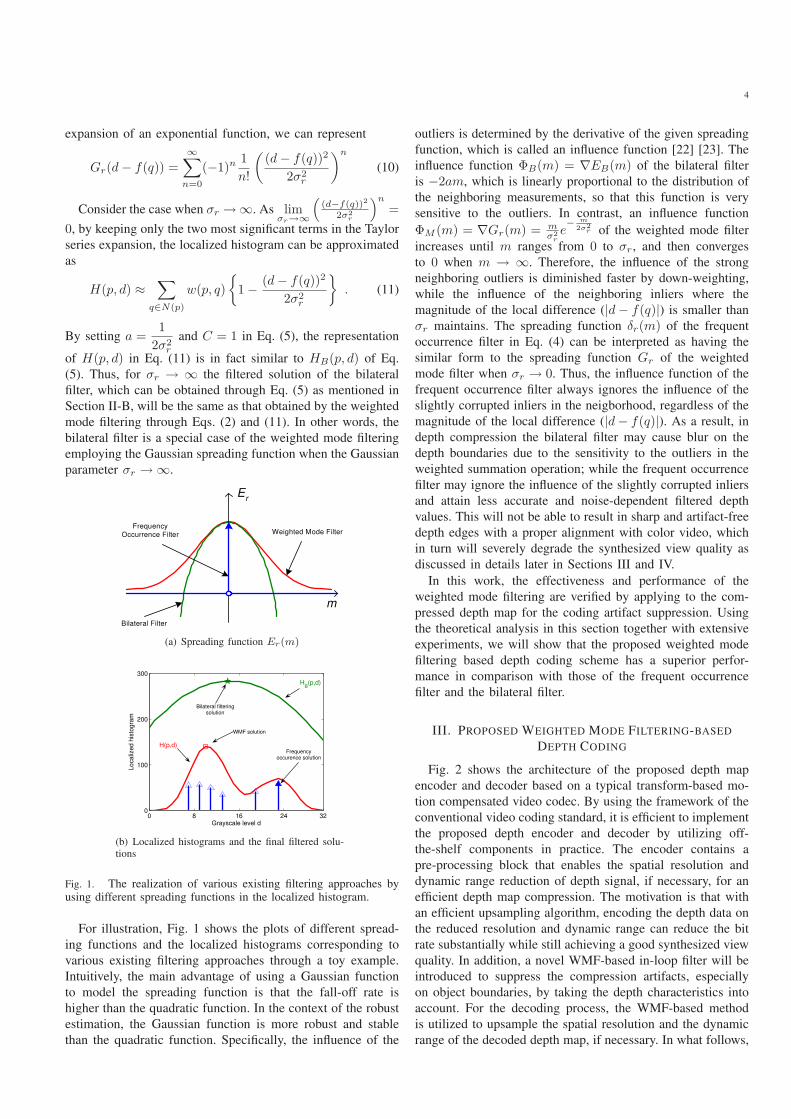
For illustration, Fig. 1 shows the plots of different spread-
ing functions and the localized histograms corresponding to
various existing filtering approaches through a toy example.
Intuitively, the main advantage of using a Gaussian function
to model the spreading function is that the fall-off rate is
higher than the quadratic function. In the context of the robust
estimation, the Gaussian function is more robust and stable
than the quadratic function. Specifically, the influence of the
outliers is determined by the derivative of the given spreading
function, which is called an influence function [22] [23]. The
influence function ΦB(m) = ∇EB(m) of the bilateral filter
is −2am, which is linearly proportional to the distribution of
the neighboring measurements, so that this function is very
sensitive to the outliers. In contrast, an influence function
ΦM (m) = ∇Gr(m) = mσ2
r
e−
m
2σ2r of the weighted mode filter
increases until m ranges from 0 to σr, and then converges
to 0 when m → ∞. Therefore, the influence of the strong
neighboring outliers is diminished faster by down-weighting,
while the influence of the neighboring inliers where the
magnitude of the local difference (|d − f(q)|) is smaller than
σr maintains. The spreading function δr(m) of the frequent
occurrence filter in Eq. (4) can be interpreted as having the
similar form to the spreading function Gr of the weighted
mode filter when σr → 0. Thus, the influence function of the
frequent occurrence filter always ignores the influence of the
slightly corrupted inliers in the neigborhood, regardless of the
magnitude of the local difference (|d − f(q)|). As a result, in
depth compression the bilateral filter may cause blur on the
depth boundaries due to the sensitivity to the outliers in the
weighted summation operation; while the frequent occurrence
filter may ignore the influence of the slightly corrupted inliers
and attain less accurate and noise-dependent filtered depth
values. This will not be able to result in sharp and artifact-free
depth edges with a proper alignment with color video, which
in turn will severely degrade the synthesized view quality as
discussed in details later in Sections III and IV.
In this work, the effectiveness and performance of the
weighted mode filtering are verified by applying to the com-
pressed depth map for the coding artifact suppression. Using
the theoretical analysis in this section together with extensive
experiments, we will show that the proposed weighted mode
filtering based depth coding scheme has a superior perfor-
mance in comparison with those of the frequent occurrence
filter and the bilateral filter.
III. PROPOSED WEIGHTED MODE FILTERING-BASED
DEPTH CODING
Fig. 2 shows the architecture of the proposed depth map
encoder and decoder based on a typical transform-based mo-
tion compensated video codec. By using the framework of the
conventional video coding standard, it is efficient to implement
the proposed depth encoder and decoder by utilizing off-
the-shelf components in practice. The encoder contains a
pre-processing block that enables the spatial resolution and
dynamic range reduction of depth signal, if necessary, for an
efficient depth map compression. The motivation is that with
an efficient upsampling algorithm, encoding the depth data on
the reduced resolution and dynamic range can reduce the bit
rate substantially while still achieving a good synthesized view
quality. In addition, a novel WMF-based in-loop filter will be
introduced to suppress the compression artifacts, especially
on object boundaries, by taking the depth characteristics into
account. For the decoding process, the WMF-based method
is utilized to upsample the spatial resolution and the dynamic
range of the decoded depth map, if necessary. In what follows,

5
Spatial Down
Sampling
Dynamic Range
Reduction
Transform
Proposed In-
loop Filter
Motion
Compensation
Intra-frame
Prediction
Entropy
Coding
Motion
Estimation
Intra/Inter
Quantization
Inverse
Transform
Inverse
Quantization
Memory
Motio
n In
form
atio
n
Depth map
Color video
Preprocessing
M bitsN bits
(M > N)
Encoder
(a) Encoder
EntropyDecoding
Inverse
Quantization
Inverse
Transform
MotionCompensation
Frame
Memory
Compresseddepth
Decoder
Proposed In-loop Filter
WMF-Based
Upsampling
Dynamic RangeIncrease
Postprocessing
Ouput depth
Color video
M bitsN bits
(M > N)
(b) Decoder
Fig. 2. Block diagrams of the proposed weighted mode filteringbased depth map encoder and decoder using a typical transform-basedmotion compensated coding scheme.
we present the three key components of our proposed depth
map encoder and decoder: (1) WMF-based in-loop filter, (2)
WMF-based spatial resolution upsampling, and (3) WMF-
based dynamic range upsampling.
A. In-loop Filter
Containing homogeneous regions separated by sharp edges,
transform-based compressed depth map often exhibits large
coding artifacts such as ringing artifacts and blurriness along
the depth boundaries. These artifacts in turn severely degrade
the visual quality of the synthesized view. Fig. 3 shows the
sample frames of the depth video compressed at different
quantization parameters (QPs) and the corresponding syn-
thesized view. Obviously, coding artifacts introduced in the
compressed depth create many annoying visual artifacts in the
virtual view, especially along the object boundaries.
Existing in-loop filters such as the H.264/AVC deblocking
filter and Wiener filter [24], which are mainly designed for
the color video, may not be suitable for the depth map
compression with different characteristics. In this paper, the
weighted mode filtering concept is employed to design an
in-loop edge-preserving denoising filter. In addition, we also
Fig. 3. Sample frames of the depth video compressed at differentQPs and the corresponding synthesized view.
extend the concept to use a guided function g(p) different
from the function f(p) to be filtered in the weighting term as
follows:
H(p, d) =∑
q∈N(p)
w(p, q)Gr(d − f(q)) (12)
w(p, q) = Gg(g(p) − g(q))Gf (f(p) − f(q))Gs(p − q)
where two range kernels Gg and Gf are introduced here to
measure a similarity between data of two pixels p and q, Gs
is the spatial kernel to indicate the geometric closeness. By
selecting such weighting function, the weighted mode filtering
is contextually similar to joint bilateral and trilateral filtering
methods [26], [27], since the guided function g(p) and the
original function f(p) is used to calculate the weighting value.
Liu et al. has observed that the weighting functions Gg and
Gf may still cause unnecessary blur on the depth boundaries
due to its summation [19]. In contrast, by selecting the global
mode on the localized histogram, it may help to reduce an
unnecessary blur along the object boundaries observed in the
case of the bilateral filtering. We will show the depth video
coding based on the weighted mode filtering outperforms the
existing post-processing based coding methods.
In general, the compressed depth map is often transmitted
together with the associate color video in order to synthesize
the virtual view at the receiver side. In addition, two corre-
lated depth pixels along the depth boundaries usually exhibit
a strong photometric similarity in the corresponding video
pixels. Inspired by this observation, we utilize the color video
pixels I(p) as the guided function g(p) to denoise the depth
data D(p) of the original function f(p). It should be noted that
both color and depth video information can be used as guided
information in the weighting term to measure the similarity
of pixels p and q. However, through extensive experiments
it is observed that using the color video information only as
guided information generally provides a better performance in
comparison with incorporating the guided depth information in
the weighting term. This can be explained by the fact that the
input depth map already contains more serious coding artifacts
around the sharp edges than the color videos. Thus, using the
noisy input depth to guide the noise filtering of its own signal
may not be effective. In contrast, color frame consistently

6
1 3 5 7 9 1137
38
39
40
41
42
43
41.9
42.3 42.3 42.242.0
41.9
40.8
41.3 41.2 41.342.1 40.9
39.539.7 39.8 39.7 39.7 39.6
38.4
38.8 38.938.7
38.938.7
Ballet
Range sigma
Synth
esiz
ed v
iew
qualit
y(d
B)
QP = 22
QP = 25
QP = 28
QP = 31
Fig. 4. PSNR (dB) results of the synthesized view obtained byencoding the depth video at different QPs using the proposed in-loopfilter with different values of range sigma σr .
provides an effective guided information even when it is
encoded heavily lossy as shown later in the experimental
results. Furthermore, in view synthesis, the distortion in depth
pixels will result in a rendering position error. By using the
similarity of color pixels to guide the filtering process, it may
diminish the quality degradation of the synthesized view due
to the rendering position error.
In our work, we shall only utilize the color video informa-
tion as guided information in the proposed weighted mode
filtering. Specifically, the localized histogram using guided
color information can be formulated as
HI(p, d) =∑
q∈N(p)
wI(p, q)Gr(d − D(q)) (13)
where the weighting term, wI , incorporates the photometric
similarity in the corresponding color video and is defined as
wI(p, q) = GI(I(p) − I(q))Gs(p − q) (14)
The range filter of the color video, GI , is chosen as a Gaussian
filter. For a fast computation, look-up tables may be utilized
for approximating float values of Gaussian filters. Note that
the “bell” width of the spreading function Gr is controlled
by the filter parameter σr. To reduce the complexity, when
the localized histogram is computed using (13), only the dth
bin satisfying |d − D(q)| ≤ B should be updated for each
neighboring pixel q, where the threshold B is determined to
meet the condition Gr(B/2) = 0.3.
As mentioned in Section II, the width (↔ σr) is determined
by the amount of noise in the input data f(p). In addition,
the larger the value of σr is, the higher the computational
complexity is. Furthermore, too large value of σr may cause
blur on the object boundaries due to the fact that the weighted
mode filtering approaches to the solution of the bilateral
filtering as mentioned in Section II. To select an optimal value
of σr, we compressed the depth video at different QPs by
using the proposed in-loop filter in the encoder with different
values of σr. An objective performance is measured indirectly
by analyzing the quality of the synthesized view (refer to
Section IV for the simulation setup details). Fig. 4 shows
the peak-signal-to-noise ratio (PSNR) of the synthesized view
obtained by using different values of σr. The results show that
with different amounts of noise introduced by the quantization
artifact, setting σr to 3 generally provides the best synthesized
(a) Edge pixels (b) Edge blocks
Fig. 5. The edge maps obtained from the depth map of the Ballettest sequence based on the classified edge pixels and edge blocks.
view quality while maintaining low computational complexity.
Meanwhile, serious coding artifacts generally appear around
sharp edges. Thus, it may be more efficient to detect and apply
the proposed in-loop filter only to these regions for an efficient
implementation. Basically, it is adequate to determine regions
containing strong edges rather than accurate edges in the depth
video. Hence, we propose to use a simple first-order method
to detect the depth discontinuities by calculating an image
gradient. Specifically, the estimates of first-oder derivatives,
Dx and Dy , and the gradient magnitude of a pixel in the
depth map D are computed as:
Dx(m,n) = D(m,n + 1) − D(m,n − 1)
Dy(m,n) = D(m + 1, n) − D(m − 1, n) (15)
|∇D(m,n)| =√
Dx(m,n)2 + Dy(m,n)2
Each pixel of the depth map is then classified as an edge
pixel if the gradient magnitude |∇D(m,n)| is greater than a
certain threshold. We then partition the depth map into non-
overlapping blocks of N × N pixels. A block is classified
as an edge block if there exists at least a certain number of
edge pixels in the block. The proposed in-loop filter is then
applied only for the pixels in these edge blocks to reduce the
computational complexity.
Fig. 5 shows the classification of edge pixels and edge
blocks obtained by the proposed method for a depth image
of the Ballet test sequence. Conceivably, the computational
complexity gain would likely depend on the size of partitioned
blocks. Intuitively, partitioning the depth map into blocks of
smaller size would result in less total number of pixels inside
the classified edge blocks that need to be filtered. Thus, it is
expected to achieve a higher gain in complexity reduction,
but may reduce the noise removal performance. Note that
the smallest transform block size in the conventional video
coding standard is a 4 × 4 integer transform in H.264/AVC,
thus the size of partitioned blocks should not be less than 4.
In our simulation, different partitioned block sizes are used to
select an optimal trade-off between the complexity gain and
the effectiveness of artifact suppression.
B. Depth Down/Upsampling
It has been shown that a downsampled video when
compressed and later upsampled, visually beats the video
compressed directly on high resolution at a certain tar-
get bit rate [28], [29]. Based on this observation, many
have proposed to encode a resolution-reduced depth video

7
to reduce the bit rate substantially [14]–[16]. However,
down/upsampling process also introduces the serious distortion
as some high frequency information is discarded. Without a
proper down/upsampling scheme, important depth information
in the object boundary regions will be distorted and affect the
visual quality of the synthesized view. In this section, we show
how to employ the filtering scheme proposed in Section III-
A to upsample the decoded depth map while recovering the
original depth edge information.
Depth Downsampling: Traditional downsampling filter,
consisting of a low-pass filter and an interpolation filter, will
smooth the sharp edges in depth map. Here, we employ a
simple median downsampling filter proposed in [15] as:
Ddown(p) = median(Ws×s) (16)
where s is a downsampling factor and each pixel value in
the downsampled depth is selected as the median value of the
corresponding block Ws×s of size s× s in the original depth.
Depth Upsampling: The proposed weighted mode filtering
is tailored to upsample the decoded depth video. Coarse-
to-fine upsampling approach proposed in our previous work
for the depth superesolution task is employed here [20]. The
advantage of the multiscale upsampling approach is to prevent
an aliasing effect in the final depth map. For simplicity, let s =2K and the upsampling will be performed in K steps. Initially,
only pixels at position p | p%2K = 0 in the upsampled depth
will be initialized from the downsampled depth as:
Dup(p | p%2K = 0) = Ddown(p/2K) (17)
The other missing pixels will be gradually initialized and
refined in every step by applying the proposed weighted mode
filtering scheme. Specifically, at step 0 ≤ k ≤ K − 1, pixels
at positions p | p%2k = 0 will be updated. Note that only
pixel q in the neighboring pixels N(p) that is initialized in
the previous steps will be re-used to compute the localized
histogram. In addition, the size of the neighboring window
N(p) will be reduced by half in each step.
C. Depth Dynamic Range Reduction
For the dynamic range of the depth map, we propose to
design a similar approach to the spatial down/upsampling
method to further reduce the encoding bit rate. The basic idea
is to first reduce the number of bits per depth sample prior to
encoding and then reconstruct the original dynamic range after
decoding. The main motivation is that the depth map consists
of less texture details compared with the color video, enabling
us to reconstruct efficiently the original dynamic range of the
depth map from the lower dynamic range data. In addition,
there exists a close relationship among depth sample, camera
baseline, and image resolution. For instance, small number of
bits per sample is sufficient to represent the depth map well
at low spatial resolution and provide a seamless synthesized
view [33]. As dynamic range reduction will severely reduce the
depth precision, an appropriate upscaling technique is required
to retain the important depth information (e.g., precision on
the depth edge) without spreading the coding artifacts from
the compressed range-reduced depth map.
Considering the above, we design a new down/upscaling
approach for the dynamic range compression. In the down-
scaling process, a simple linear tone mapping is employed to
reduce the number of bits per depth sample prior to encoding
as shown in the pre-processing block of Fig. 2. The new depth
sample value is computed as:
DN bits(p) =
⌊
DM bits(p)
2M−N
⌋
(18)
where ⌊·⌋ denotes the floor operator, M and N specify the
original and new number of bits per depth sample, respectively.
In our simulation, M is equal to 8.
The upscaling process consists of two parts; an initialization
of the downscaled depth map and the weighted mode filtering
based upscaling scheme. At first, a linear inverse tone mapping
is used to obtain an initial depth map with the original dynamic
range as follows:
DrecM bits(p) = Drec
N bits(p) ∗ 2M−N (19)
The weighted mode filtering is then applied to reconstruct
a final solution f̂(p) with the original dynamic range. By
using the guided color information, the weighted mode fil-
tering may suppress the distortion from the dynamic range
down/upscaling process by filtering the upscaling depth value
based on the neighborhood information without degrading
much the synthesized view quality. In addition, the weighted
mode filtering will also reduce the spread of any coding
artifacts in the compressed range-reduced depth map into the
reconstructed depth map at the original dynamic range. Note
that since less information is presented in the low dynamic
range, we also apply the upscaling process in the multiscale
manner. Specifically, we increase the number of bits per depth
sample by only 1 in each step and apply the proposed weighted
mode filtering. For example, we obtain 7-bit depth data in
an immediate step when reconstructing 8-bit depth from 6-bit
depth.
IV. EXPERIMENTAL RESULTS
We have conducted a series of experiments to evaluate
the performance of the proposed depth compression tech-
niques. We have tested with the Breakdancers and Ballet test
sequences with resolutions of 1024 × 768, of which both
the color video and depth map are provided from Microsoft
Research [30].
The experiments were conducted by using the H.264/AVC
Joint Model Reference Software JM17.2 to encode the depth
map of each view independently [31]. The conventional
H.264/AVC deblocking filter in the reference software was re-
placed with the proposed in-loop filter. For each test sequence,
we encoded two (left and right) views for both color and depth
videos using various QPs.
To measure the performance of the proposed method, we an-
alyzed the quality of the color information for the synthesized
intermediate view. Among 8 views, view 3 and view 5 were
selected as reference views and a virtual view 4 was generated
using the View Synthesis Reference Software (VSRS) 3.0
provided by MPEG [32]. For an objective comparison, the
8
PSNR of each virtual view generated using compressed depth
maps was computed with respect to that generated using the
original depth map. Rate distortion (RD) curves were obtained
by the total bit rate required to encode the depth maps of both
reference views and the PSNR of the synthesized view. Note
that the captured original view at the synthesis position was
not used here as a reference to measure the quality of the
virtual view since such measure generally incorporates more
than one source of distortion. For instance, there are a lot of
distortion sources such as slightly different camera response
function, exposure time, and lighting condition among multi-
view images. It has also been shown in [34] that the distortion
introduced by VSRS widely masks those due to depth map
compression, which can result in a misleading study in order
to justify the effectiveness of depth compression.
A. In-loop Filter
In the first set of experiments, we evaluated the performance
of the proposed in-loop filter in comparison with the existing
in-loop filters. Besides the conventional H.264/AVC deblock-
ing filter, we have also compared with the depth boundary
reconstruction filter [17] and the trilateral filter [19], which
are also utilized as the in-loop filter. In addition, to evaluate
the effectiveness of using the weighted mode filtering as an
in-loop filter, we have also implemented it as an out-loop
filter, in which the weighted mode filtering is applied to
the decoded depth map at the receiver side. Note that the
H.264/AVC deblocking filter was completely replaced by the
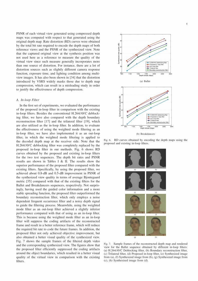
proposed in-loop filter in our methods. Fig. 6 shows RD
curves obtained by the proposed and existing in-loop filters
for the two test sequences. The depth bit rates and PSNR
results are shown in Tables I & II. The results show the
superior performance of the proposed filter compared with the
existing filters. Specifically, by using the proposed filter, we
achieved about 0.8-dB and 0.5-dB improvement in PSNR of
the synthesized view quality in terms of average Bjontegaard
metric [35] compared with that of the existing filters for the
Ballet and Breakdancers sequences, respectively. Not surpris-
ingly, having used the guided color information and a more
stable spreading function, the proposed filter outperformed the
boundary reconstruction filter, which only employs a noise
dependent frequent occurrence filter and a noisy depth signal
to guide the filtering process. Meanwhile, using the weighted
mode filter as an out-loop filter achieved a slightly inferior
performance compared with that of using as an in-loop filter.
This is because using the weighted mode filter as an in-loop
filter will suppress the coding artifacts of the reconstructed
frame and result in a better reference frame, which will reduce
the required bit rate to code the future frames. In addition, the
proposed filter not only achieved objective improvement, but
also obtained a better visual quality of the synthesized view.
Fig. 7 shows the sample frames of the filtered depth video
and the corresponding synthesized view. The figures show that
the proposed filter efficiently suppressed the coding artifacts
around the object boundaries, which resulted in a better visual
quality of the virtual view in comparison with the existing
filters.
800 1100 1400 1700 2000 2300 260037
38
39
40
41
42
43
Depth bitrate (kbps)
Synth
esiz
ed v
iew
qualit
y (
dB
)
H.264/AVC deblocking filter
Proposed in−loop filter
Out−loop filter
Trilateral filter
Boundary reconstruction filter
(a) Ballet
800 1100 1400 1700 2000 2300 260040
41
42
43
44
45
Depth bitrate (kbps)
Synth
esiz
ed v
iew
qualit
y (
dB
)
H.264/AVC deblocking filter
Proposed in−loop filter
Out−loop filter
Trilateral filter
Boundary reconstruction filter
(b) Breakdancers
Fig. 6. RD curves obtained by encoding the depth maps using theproposed and existing in-loop filters.
(a) (b)
(c) (d)
(e) (f)
(g) (h)
Fig. 7. Sample frames of the reconstructed depth map and renderedview for the Ballet sequence obtained by different in-loop filters:(a) H.264/AVC Deblocking filter, (b) Boundary reconstruction filter,(c) Trilateral filter, (d) Proposed in-loop filter, (e) Synthesized imagefrom (a), (f) Synthesized image from (b), (g) Synthesized image from(c), (h) Synthesized image from (d).
9
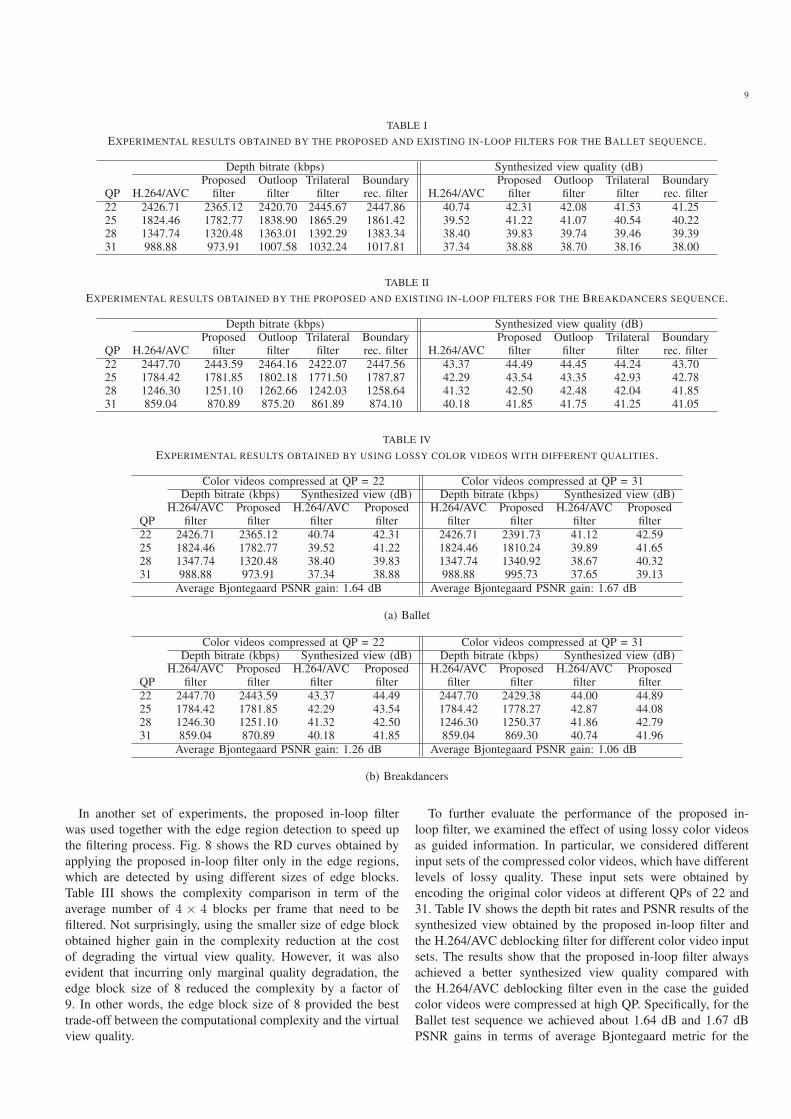
TABLE I
EXPERIMENTAL RESULTS OBTAINED BY THE PROPOSED AND EXISTING IN-LOOP FILTERS FOR THE BALLET SEQUENCE.
Depth bitrate (kbps) Synthesized view quality (dB)Proposed Outloop Trilateral Boundary Proposed Outloop Trilateral Boundary
QP H.264/AVC filter filter filter rec. filter H.264/AVC filter filter filter rec. filter
22 2426.71 2365.12 2420.70 2445.67 2447.86 40.74 42.31 42.08 41.53 41.2525 1824.46 1782.77 1838.90 1865.29 1861.42 39.52 41.22 41.07 40.54 40.2228 1347.74 1320.48 1363.01 1392.29 1383.34 38.40 39.83 39.74 39.46 39.3931 988.88 973.91 1007.58 1032.24 1017.81 37.34 38.88 38.70 38.16 38.00
TABLE II
EXPERIMENTAL RESULTS OBTAINED BY THE PROPOSED AND EXISTING IN-LOOP FILTERS FOR THE BREAKDANCERS SEQUENCE.
Depth bitrate (kbps) Synthesized view quality (dB)Proposed Outloop Trilateral Boundary Proposed Outloop Trilateral Boundary
QP H.264/AVC filter filter filter rec. filter H.264/AVC filter filter filter rec. filter
22 2447.70 2443.59 2464.16 2422.07 2447.56 43.37 44.49 44.45 44.24 43.7025 1784.42 1781.85 1802.18 1771.50 1787.87 42.29 43.54 43.35 42.93 42.7828 1246.30 1251.10 1262.66 1242.03 1258.64 41.32 42.50 42.48 42.04 41.8531 859.04 870.89 875.20 861.89 874.10 40.18 41.85 41.75 41.25 41.05
TABLE IV
EXPERIMENTAL RESULTS OBTAINED BY USING LOSSY COLOR VIDEOS WITH DIFFERENT QUALITIES.
Color videos compressed at QP = 22 Color videos compressed at QP = 31Depth bitrate (kbps) Synthesized view (dB) Depth bitrate (kbps) Synthesized view (dB)
H.264/AVC Proposed H.264/AVC Proposed H.264/AVC Proposed H.264/AVC ProposedQP filter filter filter filter filter filter filter filter
22 2426.71 2365.12 40.74 42.31 2426.71 2391.73 41.12 42.5925 1824.46 1782.77 39.52 41.22 1824.46 1810.24 39.89 41.6528 1347.74 1320.48 38.40 39.83 1347.74 1340.92 38.67 40.3231 988.88 973.91 37.34 38.88 988.88 995.73 37.65 39.13
Average Bjontegaard PSNR gain: 1.64 dB Average Bjontegaard PSNR gain: 1.67 dB
(a) Ballet
Color videos compressed at QP = 22 Color videos compressed at QP = 31Depth bitrate (kbps) Synthesized view (dB) Depth bitrate (kbps) Synthesized view (dB)
H.264/AVC Proposed H.264/AVC Proposed H.264/AVC Proposed H.264/AVC ProposedQP filter filter filter filter filter filter filter filter
22 2447.70 2443.59 43.37 44.49 2447.70 2429.38 44.00 44.8925 1784.42 1781.85 42.29 43.54 1784.42 1778.27 42.87 44.0828 1246.30 1251.10 41.32 42.50 1246.30 1250.37 41.86 42.7931 859.04 870.89 40.18 41.85 859.04 869.30 40.74 41.96
Average Bjontegaard PSNR gain: 1.26 dB Average Bjontegaard PSNR gain: 1.06 dB
(b) Breakdancers
In another set of experiments, the proposed in-loop filter
was used together with the edge region detection to speed up
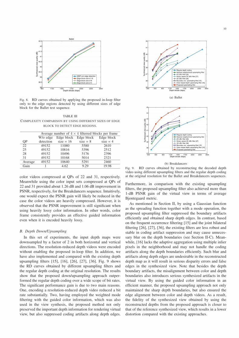
the filtering process. Fig. 8 shows the RD curves obtained by
applying the proposed in-loop filter only in the edge regions,
which are detected by using different sizes of edge blocks.
Table III shows the complexity comparison in term of the
average number of 4 × 4 blocks per frame that need to be
filtered. Not surprisingly, using the smaller size of edge block
obtained higher gain in the complexity reduction at the cost
of degrading the virtual view quality. However, it was also
evident that incurring only marginal quality degradation, the
edge block size of 8 reduced the complexity by a factor of
9. In other words, the edge block size of 8 provided the best
trade-off between the computational complexity and the virtual
view quality.
To further evaluate the performance of the proposed in-
loop filter, we examined the effect of using lossy color videos
as guided information. In particular, we considered different
input sets of the compressed color videos, which have different
levels of lossy quality. These input sets were obtained by
encoding the original color videos at different QPs of 22 and
31. Table IV shows the depth bit rates and PSNR results of the
synthesized view obtained by the proposed in-loop filter and
the H.264/AVC deblocking filter for different color video input
sets. The results show that the proposed in-loop filter always
achieved a better synthesized view quality compared with
the H.264/AVC deblocking filter even in the case the guided
color videos were compressed at high QP. Specifically, for the
Ballet test sequence we achieved about 1.64 dB and 1.67 dB
PSNR gains in terms of average Bjontegaard metric for the
10
800 1100 1400 1700 2000 2300 260038
38.5
39
39.5
40
40.5
41
41.5
42
42.5Ballet
Depth bitrate (kbps)
Synth
esiz
ed v
iew
qualit
y (
dB
)
WMF w/o edge detection
Edge block size of 16
Edge block size of 8
Edge block size of 4
Fig. 8. RD curves obtained by applying the proposed in-loop filteronly to the edge regions detected by using different sizes of edgeblock for the Ballet test sequence.
TABLE III
COMPLEXITY COMPARISON BY USING DIFFERENT SIZES OF EDGE
BLOCK TO DETECT EDGE REGIONS.
Average number of 4× 4 filterred blocks per frameW/o edge Edge block Edge block Edge block
QP detection size = 16 size = 8 size = 4
22 49152 11080 5580 261025 49152 10816 5396 251228 49152 10496 5176 239631 49152 10168 5014 2321
Average 49152 10640 5291 2460
Gain 1 4.62 9.29 19.98
color videos compressed at QPs of 22 and 31, respectively.
Meanwhile using the color input sets compressed at QPs of
22 and 31 provided about 1.26 dB and 1.06 dB improvement in
PSNR, respectively, for the Breakdancers sequence. Intuitively,
one would expect the PSNR gain will likely be reduced in the
case the color videos are heavily compressed. However, it is
observed that the PSNR improvement is still significant when
using heavily lossy color information. In other words, color
frame consistently provides an effective guided information
even when it is encoded heavily lossy.
B. Depth Down/Upsampling
In this set of experiments, the input depth maps were
downsampled by a factor of 2 in both horizontal and vertical
directions. The resolution-reduced depth videos were encoded
without enabling the proposed in-loop filter. In addition, we
have also implemented and compared with the existing depth
upsampling filters [15], [16], [26], [27], [36]. Fig. 9 shows
the RD curves obtained by different upsampling filters and
the regular depth coding at the original resolution. The results
show that the proposed down/upsampling approach outper-
formed the regular depth coding over a wide scope of bit rates.
The significant performance gain is due to two main reasons.
One, encoding a resolution-reduced depth video reduced a bit
rate substantially. Two, having employed the weighted mode
filtering with the guided color information, which was also
used in the view synthesis, the proposed method not only
preserved the important depth information for rendering virtual
view, but also suppressed coding artifacts along depth edges.
200 500 800 1100 1400 1700 2000 2300 260035
36
37
38
39
40
41
42
Depth bitrate (kbps)
Syn
the
siz
ed
vie
w q
ua
lity (
dB
)
Regular depth coding
Nearest neighborhood upsampling filter
2D JBU filter [26]
Noise−aware 2D JBU filter [27]
3D JBU filter [36]
Boundary rec. upsampling filter [15]
View−based depth upsampling filter [16]
Proposed upsampling filter
(a) Ballet
200 500 800 1100 1400 1700 2000 2300 260037
38
39
40
41
42
43
44
45
Depth bitrate (kbps)
Syn
the
siz
ed
vie
w q
ua
lity (
dB
)
Regular depth coding
Nearest neighborhood upsampling filter
2D JBU filter [26]
Noise−aware 2D JBU filter [27]
3D JBU filter [36]
Boundary rec. upsampling filter [15]
View−based depth upsampling filter [16]
Proposed upsampling filter
(b) Breakdancers
Fig. 9. RD curves obtained by reconstructing the decoded depthvideo using different upsampling filters and the regular depth codingat the original resolution for the Ballet and Breakdancers sequences.
Furthermore, in comparison with the existing upsampling
filters, the proposed upsampling filter also achieved more than
1-dB PSNR gain of the virtual view in terms of average
Bjontegaard metric.
As mentioned in Section II, by using a Gaussian function
as the spreading function together with a mode operation, the
proposed upsampling filter suppressed the boundary artifacts
efficiently and obtained sharp depth edges. In contrast, based
on the frequent occurrence filtering [15] and the joint bilateral
filtering [26], [27], [36], the existing filters are less robust and
stable in coding artifact suppression and may cause unneces-
sary blur on the depth boundaries (see Section II-C). Mean-
while, [16] lacks the adaptive aggregation using multiple inlier
pixels in the neighborhood and may not handle the coding
artifacts along the depth boundaries efficiently. Such blur and
artifacts along depth edges are undesirable in the reconstructed
depth map as it will result in serious disparity errors and false
edges in the synthesized view. Note that besides the depth
boundary artifacts, the misalignment between color and depth
boundaries also introduces serious synthesized artifacts in the
virtual view. By using the guided color information in an
efficient manner, the proposed upsampling approach not only
maintained the sharp depth boundaries, but also ensured the
edge alignment between color and depth videos. As a result,
the fidelity of the synthesized view obtained by using the
reconstructed depths from the proposed approach is closer to
that of the reference synthesized view, which results in a lower
distortion compared with the existing approaches.
11
0 200 400 600 800 1000 120036
37
38
39
40
41
42
43
44
45
46
Depth bitrate (kbps)
Syn
the
siz
ed
vie
w q
ua
lity (
dB
)
Regular depth coding
Nearest neighborhood upsampling filter
2D JBU filter [26]
Noise−aware 2D JBU filter [27]
3D JBU filter [36]
Boundary rec. upsampling filter [15]
View−based depth upsampling filter [16]
Proposed upsampling filter
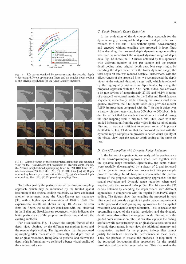
Fig. 10. RD curves obtained by reconstructing the decoded depthvideo using different upsampling filters and the regular depth codingat the original resolution for the Undo-Dancer sequence.
(a) (b)
(e) (f) (g) (h)
(c) (d)
(a) (b) (c) (d)
(e) (f) (g) (h)
Fig. 11. Sample frames of the reconstructed depth map and renderedview for the Breakdancers test sequence: (a) Regular depth coding,(b) Nearest neighborhood upsampling filter, (c) 2D JBU filter [26],(d) Noise-aware 2D JBU filter [27], (e) 3D JBU filter [36], (f) Depthupsampling boundary reconstruction filter [15], (g) View-based depthupsampling filter [16], (h) Proposed upsampling filter.
To further justify the performance of the down/upsampling
approach, which may be influenced by the limited spatial
resolution of the original coding materials, we have conducted
another experiment using the Undo-Dancer test sequence
[37] with a higher spatial resolution of 1920 × 1088. The
experimental results are shown in Fig. 10. As can be seen
from the figure, the results are consistent with that observed
in the Ballet and Breakdancers sequences, which indicates the
better performance of the proposed method compared with the
existing methods.
For visualization, Fig. 11 shows the sample frames of the
depth video obtained by the different upsampling filters and
the regular depth coding. The figures show that the proposed
upsampling filter reconstructed efficiently the depth map at
the original resolution. Being able to preserve and recover the
depth edge information, we achieved a better visual quality of
the synthesized view.
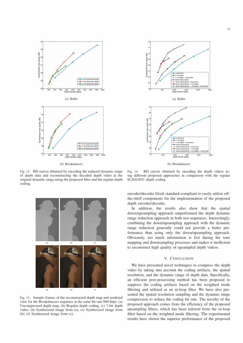
C. Depth Dynamic Range Reduction
In the evaluation of the down/upscaling approach for the
dynamic range, the original bit depths of the depth video were
reduced to 6 bits and 7 bits without spatial downsampling
and encoded without enabling the proposed in-loop filter.
After decoding, the proposed depth dynamic range upscaling
was used to reconstruct the original dynamic range of depth
data. Fig. 12 shows the RD curves obtained by this approach
with different number of bits per sample and the regular
depth coding using original depth data. Not surprisingly, by
encoding the depth video with the lower dynamic range, the
total depth bit rate was reduced notably. Furthermore, with the
effectiveness of the proposed filter, we reconstructed the depth
video at the original dynamic range well, which is reflected
by the high-quality virtual view. Specifically, by using the
proposed approach with the 7-bit depth video, we achieved
a bit rate savings of approximately 27.8% and 46.1% in terms
of average Bjontegaard metric for the Ballet and Breakdancers
sequences, respectively, while retaining the same virtual view
quality. However, the 6-bit depth video only provided modest
PSNR improvement compared with the 7-bit depth video over
a narrow bit rate range (i.e., from 200 kbps to 300 kbps). It is
due to the fact that too much information is discarded during
the tone mapping from 8 bits to 6 bits. Thus, even with the
guided information from the color video in the weighted mode
filtering, it was not sufficient to recover some of important
depth details. Fig. 13 shows that the proposed method with the
dynamic range compression provided a better visual quality of
the virtual view than the regular depth coding at the same bit
rate.
D. Down/Upsampling with Dynamic Range Reduction
In the last set of experiments, we analyzed the performance
of the down/upsampling approach when used together with
the dynamic range reduction. Specifically, the depth videos
were spatially downsampled by a factor of 2 and followed
by the dynamic range reduction process to 7 bits per sample
prior to encoding. In addition, we also evaluated the perfor-
mance of the proposed down/upsampling approaches for the
spatial resolution and dynamic range reduction when used
together with the proposed in-loop filter. Fig. 14 shows the RD
curves obtained by encoding the depth videos with different
approaches in comparison with the regular H.264/AVC depth
coding. The figures show that enabling the proposed in-loop
filter could not provide a significant performance improvement
in the proposed down/upsampling approaches for the spatial
resolution and dynamic range reduction. This is because the
upsampling stages of the spatial resolution and the dynamic
depth range also utilize the weighted mode filtering with the
guided color information. Thus, it can also suppress the coding
artifacts while reconstructing the original spatial resolution and
dynamic depth range. In our view, the additional memory and
computation required for the proposed in-loop filter cannot
justify for such an incremental performance in these cases.
Thus, we propose to disable the proposed in-loop filter in
the proposed down/upsampling approaches for the spatial
resolution and dynamic range reduction. This also makes the
12
0 200 400 600 800 1000 1200 1400 1600 1800 200034
35
36
37
38
39
40
Depth bitrate (kbps)
Synth
esiz
ed v
iew
qualit
y (
dB
)
8−bit grayscale depth
7−bit grayscale depth
6−bit grayscale depth
(a) Ballet
0 200 400 600 800 1000 1200 1400 1600 1800 200037
38
39
40
41
42
43
Depth bitrate (kbps)
Synth
esiz
ed v
iew
qualit
y (
dB
)
8−bit grayscale depth
7−bit grayscale depth
6−bit grayscale depth
(b) Breakdancers
Fig. 12. RD curves obtained by encoding the reduced dynamic rangeof depth data and reconstructing the decoded depth video at theoriginal dynamic range using the proposed filter and the regular depthcoding.
(a) (b) (c)
(d) (e) (f)
Fig. 13. Sample frames of the reconstructed depth map and renderedview for the Breakdancers sequence at the same bit rate 880 kbps: (a)Uncompressed depth map, (b) Regular depth coding, (c) 7-bit depthvideo, (d) Synthesized image from (a), (e) Synthesized image from(b), (f) Synthesized image from (c).
0 500 1000 1500 2000 250034
35
36
37
38
39
40
41
42
Depth bitrate (kbps)
Syn
the
siz
ed
vie
w q
ua
lity (
dB
)
H.264/AVC
7−bit depth
7−bit depth + inloop filter
Down/Upsampling
Down/Upsampling + inloop filter
Down/Upsampling + 7−bit depth
Down/Upsampling + 7−bit depth + inloop filter
(a) Ballet
0 500 1000 1500 2000 250037
38
39
40
41
42
43
44
45
Depth bitrate (kbps)
Syn
the
siz
ed
vie
w q
ua
lity (
dB
)
H.264/AVC
7−bit depth
7−bit depth + inloop filter
Down/Upsampling
Down/Upsampling + inloop filter
Down/Upsampling + 7−bit depth
Down/Upsampling + 7−bit depth + inloop filter
(b) Breakdancers
Fig. 14. RD curves obtained by encoding the depth videos us-ing different proposed approaches in comparison with the regularH.264/AVC depth coding.
encoder/decoder block standard-compliant to easily utilize off-
the-shelf components for the implementation of the proposed
depth encoder/decoder.
In addition, the results also show that the spatial
down/upsampling approach outperformed the depth dynamic
range reduction approach in both test sequences. Interestingly,
combining the down/upsampling approach with the dynamic
range reduction generally could not provide a better per-
formance than using only the down/upsampling approach.
Obviously, too much information is lost during the tone
mapping and downsampling processes and makes it inefficient
to reconstruct high quality of upsampled depth videos.
V. CONCLUSION
We have presented novel techniques to compress the depth
video by taking into account the coding artifacts, the spatial
resolution, and the dynamic range of depth data. Specifically,
an efficient post-processing method has been proposed to
suppress the coding artifacts based on the weighted mode
filtering and utilized as an in-loop filter. We have also pre-
sented the spatial resolution sampling and the dynamic range
compression to reduce the coding bit rate. The novelty of the
proposed approach comes from the efficiency of the proposed
upsampling filters, which has been tailored from the in-loop
filter based on the weighted mode filtering. The experimental
results have shown the superior performance of the proposed

13
filters compared with the existing filters. The proposed filters
can suppress efficiently the coding artifacts in the depth map
as well as recover depth edge information from the reduced
resolution and the low dynamic range. As a result, incurring
much lower coding bit rate, we can achieve the same quality
of the synthesized view.
ACKNOWLEDGMENT
The authors would like to thank the Associate Editor and
the reviewers for their thoughtful comments and suggestions
that helped improve the quality of this paper.
REFERENCES
[1] D. Min, D. Kim, S. Yun, and K. Sohn, “2D/3D freeview video generationfor 3DTV system,” Signal Processing: Image Communication, vol. 24,no. 1-2, pp. 31-48, 2009.
[2] MPEG document, N9760, Text of ISO/IEC 14496-10:2008/FDAM 1“Multiview Video Coding,” Oct. 2008, Busan, Korea.
[3] A. Smolic, K. Mueller, N. Stefanoski, J. Ostermann, A. Gotchev, G. B.Akar, G. Triantafyllidis, and A. Koz, “Coding Algorithms for 3DTV-ASurvey,” IEEE Trans. on Circuits and Systems for Video Technology,vol. 17, no. 11, pp. 1606-1621, 2007.
[4] MPEG document, N9992, “Results of 3D Video Expert Viewing,” Jul.2008, Hannover, Germany.
[5] MPEG document, w11061, “Applications and requirements on 3D videocoding,”MPEG, Xi’an, China, Oct. 2009.
[6] P.Kauff, N.Atzpadin, C.Fehn, M.Muller, O.Schreer, A.Smolic, and R.Tanger, “Depth map creation and image-based rendering for advanced3DTV services providing interoperability and scalability,” Signal Pro-
cessing: Image Communication, pp. 217-234, 2007.
[7] P. Merkle, A. Smolic, K. Muller, and T. Wiegand, “Multi-view videoplus depth representation and coding,” in Proc. IEEE ICIP, 2007.
[8] Y. Morvan, P. With and D. Farin, “Platelet-based coding of depth mapsfor the transmission of multiview images,” in Proc. of SPIE, Stereoscopic
Displays and Applications, vol. 6055, pp. 93-100, 2006.
[9] P. Merkle, Y. Morvan, A. Smolic, D. Farin, K. Mueller, P. With, andT. Wiegand, “The effects of multiview depth video compression onmultiview rendering,” Singal Processing: Image Communication, 2009.
[10] M. Maitre and M. N. Do, “Joint encoding of the depth image basedrepresentation using shape-adaptive wavelets,” in Proc. IEEE ICIP,2008.
[11] G. Shen, W.-S. Kim, A. Ortega, J. Lee, and H. Wey, “Edge-aware IntraPrediction for Depth-map Coding,” in Proc. IEEE ICIP, 2010.
[12] W.-S. Kim, A. Ortega, P. Lai, D. Tian, and C. Gomila, “Depth mapdistortion analysis for view rendering and depth coding,” in Proc. IEEE
ICIP, 2009.
[13] P. Lai, A. Ortega, C. C. Dorea, P. Yin, and C. Gomila, “Improving ViewRendering Quality and Coding Efficiency by Suppressing CompressionArtifacts in Depth-Image Coding,” In Proc. SPIE VCIP, 2009.
[14] E. Ekmekcioglu, M. Mrak, S. Worrall, and A. Kondoz, “Utilisationof edge adaptive upsampling in compression of depth map videos forenhanced free-viewpoint rendering,” in Proc. IEEE ICIP, 2009.
[15] K. J. Oh, S. Yea, A. Vetro, and Y. S. Ho, “Depth Reconstruction Filterand Down/Up sampling for Depth Coding in 3D Video,” IEEE Signal
Processing Letters, pp. 1-4, 2009.
[16] M. O. Wildeboer, T. Yendo, M. P. Tehrani, T. Fujii, and M. Tanimoto,“Depth Up-sampling for Depth Coding using View Information,” inProc. of 3DTV-CON, 2011.
[17] K.-J. Oh, A. Vetro, and Y.-S. Ho, “Depth Coding Using a BoundaryReconstruction Filter for 3-D Video Systems,” IEEE Trans. on Circuits
and Systems for Video Technology, vol. 21, no. 3, pp. 350-359, 2011.
[18] K.-J. Oh, S. Yea, A. Vetro, and Y.-S. Ho, “Depth Reconstruction Filterfor Depth Coding,” IEEE Electron. Lett. , vol. 45, no. 6, Mar. 2009.
[19] S. Liu, P. Lai, D. Tian, and C. W. Chen, “New Depth Coding TechniquesWith Utilization of Corresponding Video,” IEEE Trans. on Broadcast-
ing, vol. 57, no. 2, pp. 551-561, 2011.
[20] D. Min, J. Lu, and M. N. Do, “Depth Video Enhancement Based onWeighted Mode Filtering,” IEEE Trans. on Image Processing, vol. 21,no. 3, pp. 1176-1190, 2012.
[21] J. Weijer and R. Boomgaard, “Local Mode Filtering,” in IEEE Proc.
Computer Vision and Pattern Recognition, pp. 428-433, 2001.
[22] F. R. Hampel, E. M. Ronchetti, P. J. Rousseeuw, and W. A. Stahel,“Robust Statistics: The Approach Based on Influence Functions,” NewYork: Wiley, 1986.
[23] M. J. Black, G. Sapiro, D. H. Marimont, and David Heeger, “RobustAnisotropic Diffusion,” IEEE Trans. on Image Processing, vol. 7, no. 3,1998.
[24] T. Watanabe, N. Wada, G. Yasuda, A. Tanizawa, T. Chujoh, and T.Yamakage, “In-loop Filter Using Block-Based Filter Control for VideoCoding,” in Proc. IEEE ICIP, Nov. 2009.
[25] M. Elad, “On the Origin of the Bilateral Filter and Ways to Improve It,”IEEE Trans. on Image Processing, vol. 11, pp. 1141-1151, 2002.
[26] J. Kopf, M. F. Cohen, D. Lischinski and M. Uyttendaele, “Joint bilateralupsampling,” ACM SIGGRAPH 2007.
[27] D. Cham, H. Buisman, C. Theobalt, and S. Thrun, “A Noise-Aware Filterfor Real-Time Depth Upsampling,” in Proc. of Workshop on MMSFAA,2008.
[28] A. M. Bruckstein, M. Elad, and R. Kimmel, “Down-Scaling for BetterTransform Compression,” IEEE Trans. on Image Processing, vol. 12,no. 9, pp. 1132-1145, Sep. 2003.
[29] V. A. Nguyen, W. Lin, and Y. P. Tan, “Downsampling/Upsampling forBetter Video Compression at Low Bit Rate,” in Proc. IEEE ISCAS, pp.1-4, May 2008.
[30] MSR 3-D Video Sequences [Online]. Available:http://www.research.microsoft.com/vision/ImageBasedRealitites/3DVideoDownload.
[31] JM Reference Software Version 17.2http://bbs.hhi.de/suehring/tml/download.
[32] M. Tanimoto, T.Fujii, and K. Suzuki, “View synthesis algorithm inview synthesis reference software 3.0 (VSRS3.0),” Tech. Rep. DocumentM16090, ISO/IEC JTC1/SC29/WG11, Feb. 2009.
[33] K. Muller, P. Merkle, and T. Wiegand, “3-D Video Representation UsingDepth Maps,” Proceedings of the IEEE, vol. 99, no. 4, pp. 643-656, Apr.2011.
[34] N. A. El-Yamany, K. Ugur, M. M. Hannuksela, and M. Gabbouj,“Evaluation of Depth Compression and View Synthesis Distortions inMultiview-Video-Plus-Depth Coding Systems,” in IEEE Proc. 3DTV-
CON, Jun. 2010.[35] “An excel add-in for computing Bjontegaard metric and its evolution,”
document VCEG-AE07, ITU-T SG16 Q.6, Jan. 2007.[36] Q. Yang, R. Yang, J. Davis, and D. Nister, “Spatial-Depth Super
Resolution for Range Images,” in Proc. of CVPR, 2007.[37] Undo-Dancer Video Sequences. Available:
http://mpeg3dv.research.nokia.com.