Effect of Correlated LGN Firing Rates on Predictions for Monocular Eye

Closure vs Monocular Retinal Inactivation

Brian S. Blais

Department of Science and Technology, Bryant University, Smithfield RI and

Institute for Brain and Neural System s, Brown University, Providence RI

Leon N Cooper

Department of Physics, Brown University, Providence RI and

Institute for Brain and Neural Systems, Brown University, Providence RI

Harel Z. Shouval

Department of Neurobiology and Anatomy,

University of Texas Medical School at Houston, Houston TX and

Institute for Brain and Neural Systems, Brown University, Providence RI

(Dated: November 13, 2009)

Monocular deprivation experiments can be used to distinguish between different ideas

concerning properties of cortical synaptic plasticity. Monocular deprivation by lid suture

causes a rapid disconnection of the deprived eye connected to cortical neurons whereas total

inactivation of the deprived eye produces much less of an ocular dominance shift. In order

to understand these results one needs to know how lid suture and retinal inactivation affect

neurons in the lateral geniculate nucleus (LGN), that provide the cortical input. Recent

experimental results by Linden et al. (2009) show that monocular lid suture and monocular

inactivation do not change the mean firing rates of LGN neurons but that lid suture reduces

correlations between adjacent neurons whereas monocular inactivation leads to correlated

firing. These, somewhat surprising, results contradict assumptions that have been made to

explain the outcomes of different monocular deprivation protocols. Based on these experi-

mental results we modify our assumptions about inputs to cortex during different deprivation

protocols and show their implications when combined with different cortical plasticity rules.

Using theoretical analysis, random matrix theory, and simulations we show that high

levels of correlations reduce the ocular dominance shift in learning rules that depend on

homosynaptic depression (i.e. Bienenstock Cooper and Munro (BCM) type rules), consistent

with experimental results, but have the opposite effect in rules that depend on heterosynaptic

depression (i.e. Hebbian/Principal Component Analysis (PCA) type rules).

PACS numbers: 87.19.L-, 87.19.ll, 87.19.lw,

2

I. INTRODUCTION

Receptive fields in visual cortex are modifiable in the early period of an animals postnatal

development. This is thought to depend on synaptic plasticity [1, 2]; the detailed dynamics of such

receptive field modifiability has been used to infer the precise form of synaptic plasticity[3, 4]. In

a classical paradigm, called monocular deprivation (MD), vision through one eye is deprived in

early development. In this paradigm cells in visual cortex tend to disconnect from the deprived

eye [5]. We have previously shown how variants of deprivation can be used to distinguish between

different classes of learning rules: rules that depend on homosynaptic modification, such as the rule

proposed by Bienenstock Cooper and Munro (BCM)[4, 6] and rules that depend on heterosynaptic

modification [7] such as the Hebbian-based Oja rule, or PCA rule [4, 8]. Experiments have shown

that if monocular deprivation is produced by monocular lid closure (MC) then a rapid loss of

response to the deprived eye occurs, while if the retina is inactivated by an injection of TTX

(MI), significantly less loss is observed [9, 10]. These results are consistent with homosynaptic

BCM-like learning rules. However, the theoretical analysis relies on the, seemingly reasonable,

assumption that in the inactivated case (MI) activity in the lateral geniculate nucleus (LGN),

which is the cortical input, is reduced compared to the lid closure case (MC). This assumption has

been questioned by new experimental results.

In a recent study[11] the activity of neurons in LGN has been recorded during normal vision,

when the eye-lid of the experimental animals was sutured and when TTX was injected into the eye.

The recordings were conducted on awake animals while they watched movie clips and sinusoidal

gratings. The surprising result of these experiments is that MI did not reduce mean activity in

LGN when compared to MC; however MI caused an increase in correlations between different cells

within the LGN. Previous experimental results in ferret LGN [12, 13], and recent results in mouse

LGN [11] indicate that the activity of nearby cells in LGN are correlated, that this activity falls off

as a function of the distance between the receptive fields of the cells, and that these correlations

exist even in the absence of retinal activity.

In this paper we examine the impact of input correlations during deprivation experiments on

two different iconic examples of homosynaptic and heterosynaptic learning rules; BCM and PCA.

We find that the consequences of the PCA rule are inconsistent with experimental results but

that large correlations in LGN can significantly slow down the loss of response to the deprived

eye for BCM neurons in agreement with experiment. Further experimental work to quantitatively

determine the correlations within LGN in MI would permit more detailed comparison of theory

3

y!M

! ! ""2y ! ! +"1(y " #M )

!

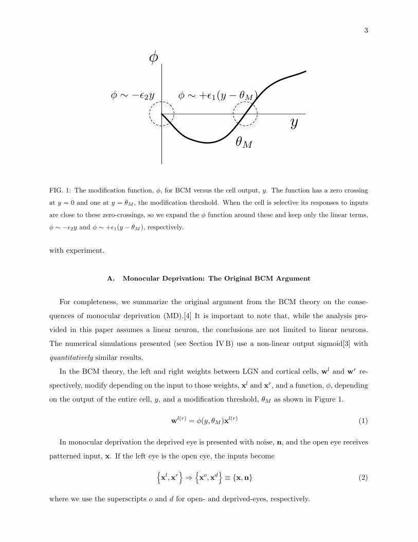
FIG. 1: The modification function, φ, for BCM versus the cell output, y. The function has a zero crossing

at y = 0 and one at y = θM , the modification threshold. When the cell is selective its responses to inputs

are close to these zero-crossings, so we expand the φ function around these and keep only the linear terms,

φ ∼ −ε2y and φ ∼ +ε1(y − θM ), respectively.

with experiment.

A. Monocular Deprivation: The Original BCM Argument

For completeness, we summarize the original argument from the BCM theory on the conse-

quences of monocular deprivation (MD).[4] It is important to note that, while the analysis pro-

vided in this paper assumes a linear neuron, the conclusions are not limited to linear neurons.

The numerical simulations presented (see Section IV B) use a non-linear output sigmoid[3] with

quantitatively similar results.

In the BCM theory, the left and right weights between LGN and cortical cells, wl and wr re-

spectively, modify depending on the input to those weights, xl and xr, and a function, φ, depending

on the output of the entire cell, y, and a modification threshold, θM as shown in Figure 1.

wl(r) = φ(y, θM )xl(r) (1)

In monocular deprivation the deprived eye is presented with noise, n, and the open eye receives

patterned input, x. If the left eye is the open eye, the inputs become

{xl,xr

}⇒{xo,xd

}≡ {x,n} (2)

where we use the superscripts o and d for open- and deprived-eyes, respectively.

4

If MD begins when the receptive fields have already reached their selective fixed points, and we

further assume (without loss of generality) that the threshold, θM , adjusts very quickly, then we

have for the open eye

wo · xoi = θM i = 1 (preferred input)

wo · xoi = 0 i > 1 (non-preferred input)(3)

where the preferred inputs are input patterns to which the neuron is selective, and the non-preferred

inputs are input patterns to which the neuron is not selective. (In a realistic environment, the actual

responses fall with some distribution peaking near zero or θM .)

Expanding φ around zero and θM , we get

φ ' +ε1(y − θM ) y near θM

φ ' −ε2y y near zero(4)

The output of the cell for the different patterns entering the open eye is

y ' θM + wd · n i = 1 (preferred input)

y ' wd · n i > 1 (non-preferred input)(5)

so that the deprived-eye weights modify as

wd '

+ε1(θM + wd · n− θM )n preferred patterns

−ε2(wd · n)n non-preferred patterns(6)

For the deprived eye, averaged over the environment and time, we have

⟨wdi

⟩' −

∑j

ε < wdjnjni >= −∑j

ε < wdj >< njni >

= −∑j

ε < wdj >< n2 > Qji (7)

where

ε ≡ −(ε2Nnon−pref − ε1Npref)/(Nnon−pref +Npref)

< n2 > = < n2i > for all i

< n2 > Qij ≡ < ninj >

5

and Npref and Nnon−pref are the number of preferred and non-preferred patterns, respectively. Note

that the diagonal elements of Q are 1.

If ni and nj are uncorrelated in space, both with mean zero

〈ninj〉 = 〈ni〉〈nj〉 = 0 when i 6= j (8)

yielding the usual result,

wdi ' −εn2wdi (9)

Thus the deprived-eye weights decrease, and decrease faster if there is more noise (i.e. higher n2)

from the deprived-eye. This deprivation effect is stronger for more selective neurons.

B. Monocular Deprivation: The Original Hebbian (PCA) Argument

The dynamics of Hebbian learning rules are determined by the eigenvectors of the correlation

matrix with the largest eigenvalues, or the principal components (PCA) [4, 14]. In one learning

rule proposed by Oja in 1982 the weight vector converges to the largest eigenvector and the length

of the vector is normalized to 1 [8]. This rule takes the form:

w = xy − y2w (10)

We now show that the monocular deprivation results cannot be obtained by a PCA learning rule

such as that of Oja, given the same assumptions about the inputs. This PCA analysis is not

restricted to this one learning rule, but is representative of a general class of Hebb-based learning

rules.[4, 14]

An exact solution to Oja’s learning rule, which is a form of PCA or stabilized Hebbian learning,

is shown by Wyatt and Elfeldel [15] to be

w(t) =eQFULLtw0

(||eQFULLtw0||2 + 1− ||w0||)12

, (11)

where w0 = w(t = 0) is the initial state of the weight vector and QFULL is the 2-eye correlation

function. We need to include the correlation for the open eye when considering PCA because both

the initial development of selectivity with this rule, and the dynamics of deprivation, depend on

the open-eye correlations.

6

1. Normal Rearing

If both eyes have exactly the same input, the 2-eye correlation function, QFULL, has the form

QFULL =

Qopen Qopen

Qopen Qopen

(12)

where Qopen is the open-eye correlation function.

We expand the initial weight vector w(0) in terms of the eigenvectors, uj , of the open-eye

correlation matrix.

w(0) =

wl(0)

wr(0)

=∑j

aljuj

arjuj

(13)

where uj , the j’th eigenvector of the one-open-eye correlation function Qopen, has the eigenvalue

ξj and alj , arj are the expansion coefficients for left and right eye respectively. We assume that

eigenvectors and eigenvalues are arranged in a descending order, that is ξ1 > ξ2 > · · · ξN . Inserting

this into the Wyatt formula, and taking the limit, we get

w(t→∞) =√

12

u1

u1

(14)

as long as the largest eigenvalue is non-degenerate.

Thus the solution converges to a state in which both eye receptive fields are eigenvectors of the

one-eye correlation function Qopen. The higher the ratio between ξ1 and the smaller eigenvalues

the faster it will converge.

2. Monocular Deprivation (MD)

As for BCM, we assume that one eye is open and generates a structured input to the cortical

cell, whereas the other eye is deprived and the activity of the deprived LGN inputs is uncorrelated

with open-eye inputs.

Thus the full correlation function has the form

QFULL =

Qopen 0

0 n2Q

(15)

7

where n2 is the variance of the deprived-eye inputs. The eigenvectors and eigenvalues of the open

and deprived-eye correlation function are defined as

(open eye) Qopenui = ξiui (16)

(deprived eye) Qvj = λjvj (17)

MD is started after the neuron has converged to the binocular fixed-point,

w(0) =√

12

u1

u1

(18)

We expand the initial condition for the deprived-eye in terms of the eigenvectors of the deprived-eye

correlation function, Q.

u1 =∑j

bjvj (19)

The deprived-eye term in the numerator of the Wyatt solution (Equation 11) using the corre-

lation function in Equation 15 is

en2Qtu1 =

∑j

en2λjtbjvj (20)

≈ en2λ1tb1v1 (21)

= en2λ1t(u1 · v1)v1 (22)

where the approximation assumes that the largest eigenvalue of the deprived-eye correlation func-

tion is larger then all of the others. In the case of a degenerate largest eigenvalue, a constant N

would multiply the term in Equation 22 and none of the conclusions that follow would change.

After this approximation, we arrive at the solution

w(t) =

eξ1tu1

en2λ1t(u1 · v1)v1

(e2ξ1t + e2n2λ1t(u1 · v1)2)1/2

(23)

If the magnitude of the deprived-eye maximum eigenvalue (scaled by the variance) is smaller

than the largest eigenvalue of the visual inputs, that is n2λ1 < ξ1, then the t → ∞ limiting case

becomes

w(t→∞) =

u1

0

(24)

8

and the deprived-eye weights decay.

The rate of decay of the deprived eye depend on the difference between the open-eye maximum

eigenvalue, ξ1, and the deprived-eye maximum eigenvalue scaled by the variance, n2λ1. Thus, the

larger the variance of the noise the slower the decay of the deprived-eye weights, which is the

opposite behavior to BCM. It is in fact possible,in the presence of very large noise, to get a PCA

neuron to have an increased response to the deprived eye and a corresponding decrease in the

open-eye responses.

II. RESULTS

A. Monocular Deprivation with BCM and Correlation of LGN Activity

We now generalize the BCM argument to deal with complex correlations in LGN activity. We

explore the possibility that lid closure (MC) leads to LGN noise that is uncorrelated, and that

retinal inactivation with TTX (MI), leads to LGN noise that is correlated resulting in a possible

decrease in the synaptic modification for inactivated inputs.

Denote

< wdi > → wi

< n2 > → n2

to obtain

wi = −∑j

εn2Qijwj (25)

In matrix form

w = −εn2Qw (26)

where Q is a square, N dimensional correlation matrix. The eigenvectors of Q are

Qvi = λivi (27)

9

We expand the weight vector in the complete set of eigenvectors,

w(t) =N∑i=1

ai(t)vi

so that

˙w(t) =N∑i=1

ai(t)vi = −εn2QN∑i=1

ai(t)vi

= −εn2N∑i=1

λiai(t)vi (28)

This gives

ai(t) = ai(0)e−εn2λit (29)

and

w(t) =N∑i=1

ai(0)e−εn2λitvi

=N∑i=1

ai(0)e−t/τivi (30)

with the time constants for the decay defined as τi = (εn2λi)−1.

The activity in LGN neurons from the deprived eye can now be characterized by the correlation

matrix, Q.

1. Uncorrelated Noise

In the original MD uncorrelated noise argument of BCM, the matrix Q is

Q→

1 0 0 0 · · ·

0 1 0 0 · · ·

0 0 1 0 · · ·

0 0 0 1 · · ·...

. . .

= I (31)

This leads to λi = 1 for all w, therefore

w(t) = w(0)e−εn2t

10

which approaches 0 as t→∞.

This is the ‘normal’ BCM uncorrelated noise result and gives the reference time of decay,

τ = (εn2)−1. Note that the weights all decay in time, with a faster decay for a larger noise

variance, n2.

2. Fully Correlated Noise

If the inputs to the deprived eye are completely correlated, Q becomes

Q→

1 1 1 1 · · ·

1 1 1 1 · · ·

1 1 1 1 · · ·...

. . .

(32)

This results in

λ1 = N for the DC eigenvector v1 =1√N

(1, 1, · · · , 1)T (33)

λ2, · · · , λN = 0 (34)

so that

w(t) = a11√N

1

1

1...

1

e−εn

2Nt +N∑i=2

ai(0)vi (35)

The first term is non-selective and decays rapidly. All of the others do not decay, τi 6=1 = ∞.

Thus, if the initial state is selective there is no decay.

3. Partial Constant Correlation

Let the inputs to the deprived eye be partially correlated so that Q is[21]

Q→

1 q q q · · ·

q 1 q q · · ·

q q 1 q · · ·...

. . .

(36)

11

We can write Q as

Q = (1− q)I + qJ (37)

where I is the identity and J is defined as

J ≡

1 1 1 1 · · ·

1 1 1 1 · · ·

1 1 1 1 · · ·...

. . .

(38)

The eigenvectors and eigenvalues of Q are

v1 = 1√N

(1, 1, 1, · · · , 1)T λ1 = 1 + (N − 1)q

vi orthogonal to v1 λi = 1− q for i > 1(39)

This gives

w(t) = a1(0)e−εn2(1+(N−1)q)tv1 +

N∑i=2

ai(0)e−εn2(1−q)tvi (40)

The first term is non-selective and decays rapidly. The other terms decay with characteristic

time τq = (εn2(1 − q))−1. Note that since τ−1q ≤ εn2, the weights decay more slowly than the

uncorrelated case, and τq reaches its maximum at q = 1, where there is no decay as in equation 35.

4. Partial Non-Uniform Correlation

We now relax the assumption that the correlation between any two neurons is a constant, q.

Let the correlation matrix have the form

Q = Q0 + Q1 (41)

where Q0 is the correlation function above,

Q0 = (1− q)I + qJ (42)

and Q1 is a symmetric, N -dimensional random-valued matrix whose off-diagonal elements have

mean zero with variance, m2

12

Q1 ≡

0 ∆ij · · ·

∆ij 0 0 · · ·...

. . .

(43)

where ∫pij(∆ij)∆2

ijd(∆ij) = m2

∆ij = ∆ji

uncorrelated indepen-

dent random variables

of the N ×N symmet-

ric matrix∫pij(∆ij)d(∆ij) = 1

Matrices such as Q1 have been analyzed by Wigner[16] and found to have the following eigen-

value distribution in the large N limit

σ(λ) =

(4Nm2−λ2)1/2

2πNm2 for λ2 < 4Nm2

0 for λ2 > 4Nm2(44)

In order to find the eigenvalues of Q we use a perturbation theory argument. In the non-

perturbed case:

Q0vi = λ0ivi

λ01 = 1 + (N − 1)q

λ02, · · · , λ0

N = 1− q

If we treat Q1 as a perturbation, in the lowest order

λα>1 = λ0α + 〈α|Q1|α〉 (45)

Because the zero-order eigenvalues are largely degenerate we must diagonalize Q1 over the degen-

erate states; but this is just the problem solved by Wigner. We can therefore add the Wigner

distribution to the unperturbed eigenvalues, λ2, · · · , λN = 1− q, to get

λ2, · · · , λN = 1− q + (Wigner distribution) (46)

13

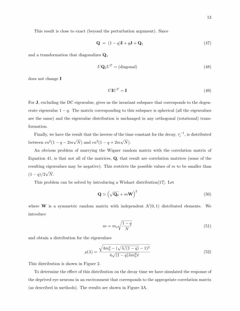
This result is close to exact (beyond the perturbation argument). Since

Q = (1− q)I + qJ + Q1 (47)

and a transformation that diagonalizes Q1

UQ1UT = (diagonal) (48)

does not change I

UIUT = I (49)

For J, excluding the DC eigenvalue, gives us the invariant subspace that corresponds to the degen-

erate eigenvalue 1− q. The matrix corresponding to this subspace is spherical (all the eigenvalues

are the same) and the eigenvalue distribution is unchanged in any orthogonal (rotational) trans-

formation.

Finally, we have the result that the inverse of the time constant for the decay, τ−1i , is distributed

between εn2(1− q − 2m√N) and εn2(1− q + 2m

√N).

An obvious problem of marrying the Wigner random matrix with the correlation matrix of

Equation 41, is that not all of the matrices, Q, that result are correlation matrices (some of the

resulting eigenvalues may be negative). This restricts the possible values of m to be smaller than

(1− q)/2√N .

This problem can be solved by introducing a Wishart distribution[17]. Let

Q '(√

Q0 +mW)2

(50)

where W is a symmetric random matrix with independent N (0, 1) distributed elements. We

introduce

m = mo

√1− qN

(51)

and obtain a distribution for the eigenvalues

ρ(λ) =

√4m2

o − (√λ/(1− q)− 1)2

4√

(1− q)λm2oπ

(52)

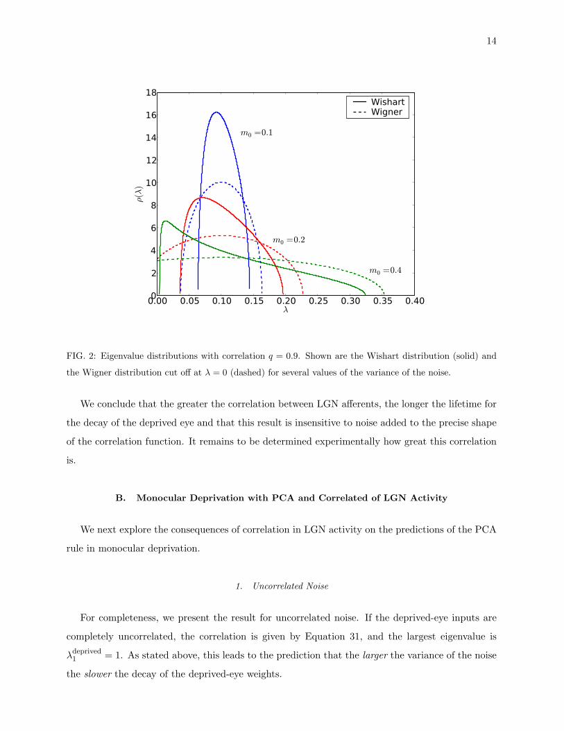
This distribution is shown in Figure 2.

To determine the effect of this distribution on the decay time we have simulated the response of

the deprived eye neurons in an environment that corresponds to the appropriate correlation matrix

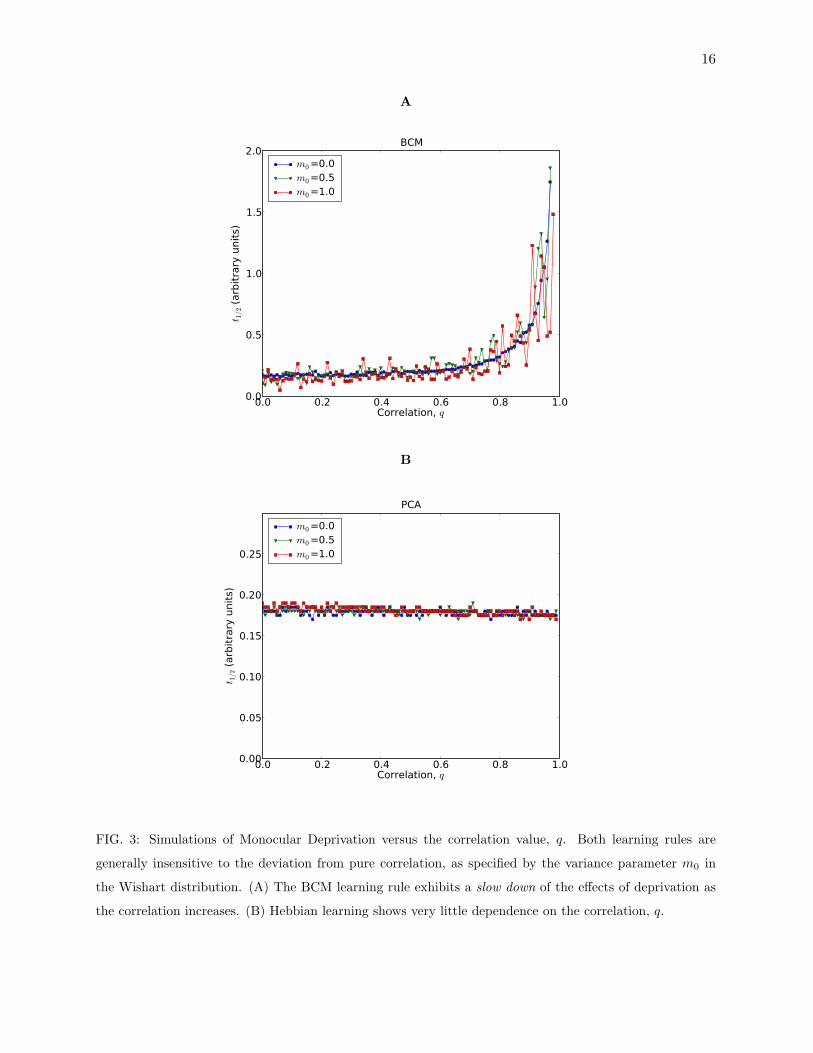
(as described in methods). The results are shown in Figure 3A.

14

0.00 0.05 0.10 0.15 0.20 0.25 0.30 0.35 0.40λ

0

2

4

6

8

10

12

14

16

18

ρ(λ

)m0 =0.1

m0 =0.2

m0 =0.4

WishartWigner

FIG. 2: Eigenvalue distributions with correlation q = 0.9. Shown are the Wishart distribution (solid) and

the Wigner distribution cut off at λ = 0 (dashed) for several values of the variance of the noise.

We conclude that the greater the correlation between LGN afferents, the longer the lifetime for

the decay of the deprived eye and that this result is insensitive to noise added to the precise shape

of the correlation function. It remains to be determined experimentally how great this correlation

is.

B. Monocular Deprivation with PCA and Correlated of LGN Activity

We next explore the consequences of correlation in LGN activity on the predictions of the PCA

rule in monocular deprivation.

1. Uncorrelated Noise

For completeness, we present the result for uncorrelated noise. If the deprived-eye inputs are

completely uncorrelated, the correlation is given by Equation 31, and the largest eigenvalue is

λdeprived1 = 1. As stated above, this leads to the prediction that the larger the variance of the noise

the slower the decay of the deprived-eye weights.

15

2. Partial Constant Correlation

If the input correlations to the deprived-eye are of the form in Equation 36 then we know the

eigenvectors and eigenvalues, given in Equation 39. If the initial (selective) one-eye vector, u1 has

no DC component (i.e. u1 · (1, 1, 1, · · ·) = 0) then the numerator term of the deprived-eye Wyatt

solution (20) becomes

∑j

en2λjt(u1 · vj)vj = en

2(1−q)t∑j

(u1 · vj)vj (53)

= en2(1−q)tu1 (54)

Thus the Wyatt solution yields

wMI(t) =

wopen(t)

wdeprived(t)

=

eξ1tu1

en2(1−q)tu1

(e2ξ1t + e2n2(1−q)t)1/2

(55)

which will result in the decay of the deprived-eye weights if ξ1 > n2(1−q), where ξ1 comes from

the natural images. In the special case that ξ1 � n2, the deprived-eye weights decay exponentially

||wdeprived|| ∼ exp(−ξ1t) (56)

The largest eigenvalue, ξ1, coming from the natural images tends to be large compared to

n2(1 − q) (on the order of 10), thus there is very little dependence on q, as seen in Figure 3. In

practice there is a small DC component due to the finite size of the receptive field, which would

grow exponentially, but the test stimulus does not register any changes due to the DC component

of the receptive field.

3. Partial Correlation with Variance

It follows from Wigner’s work on stochastic matrices, explored in Section II A 4, if the correlation

function from Equation 36 is perturbed with random components, the distribution of eigenvalues

has a maximum value of λ < 2 − 2q before the distribution becomes partly negative and we no

longer have a correlation matrix. Generalizing this to the Wishart distribution, we can obtain

eigenvectors with larger eigenvalues. In practice, however, this has little effect.(Figure 3)

16

A

0.0 0.2 0.4 0.6 0.8 1.0Correlation, q

0.0

0.5

1.0

1.5

2.0

t 1/2

(arb

itra

ry u

nit

s)

BCM

m0 =0.0m0 =0.5m0 =1.0

B

0.0 0.2 0.4 0.6 0.8 1.0Correlation, q

0.00

0.05

0.10

0.15

0.20

0.25

t 1/2

(arb

itra

ry u

nit

s)

PCA

m0 =0.0m0 =0.5m0 =1.0

FIG. 3: Simulations of Monocular Deprivation versus the correlation value, q. Both learning rules are

generally insensitive to the deviation from pure correlation, as specified by the variance parameter m0 in

the Wishart distribution. (A) The BCM learning rule exhibits a slow down of the effects of deprivation as

the correlation increases. (B) Hebbian learning shows very little dependence on the correlation, q.

17

III. DISCUSSION

The BCM theory [4, 6] makes the testable prediction that the ocular dominance shift due to lid

closure (MC) is more rapid than that due to retinal inactivation with TTX (MI). This prediction

motivated the experiment of Rittenhouse et al (1999) that attempted to test the noise-dependence

of loss of deprived-eye response by comparing MC with MI (produced by injecting TTX into the

retina of the deprived eye shutting down retinal neuronal activity). It was implicitly assumed in

this study that shutting down retinal activity would reduce LGN noise to cortical cells. The results

of Rittenhouse et al (1999) were in accord with the BCM prediction: MI showed a much slower loss

of response to the deprived eye than MC. These results were confirmed and expanded in studies in

mice[10]. But this prediction of BCM was based on the assumption that retinal inactivation would

reduce the activity level in the layers of LGN corresponding to the inactivated eye.

The study of Linden et al 2009 was done to directly check the assumption that TTX reduction

of retinal activity actually reduced LGN activity. Instead it was found that LGN activity is not

reduced on average but becomes highly correlated. These results require a reexamination of the

analysis and the expected results of different deprivation experiments in the BCM theory as well

as in other theories of synaptic plasticity [4].

Our present study was initiated to investigate the consequences on the BCM and the PCA

theories for MC vs MI in situations when retinal inactivation leads to LGN noise that is not

reduced but is correlated. We note that theoreticians had not investigated this previously because

no one thought this would be a consequence of TTX retinal inactivation: a wonderful reminder

that the real world produces surprises most of us would not expect.

Our present analysis shows that the BCM theory in the situation where the average noise

activity is unchanged[11] predicts a reduced loss of response of the inactivated eye (compared to

lid closure) that depends on the amount of correlation between firing rates of LGN neurons. For

zero correlation and identical noise variance, MI would produce the same loss as MC. But for total

correlation, there is no loss at all! In contrast we find that in the PCA theory the magnitude of

the noise correlations does not significantly effect the time course of deprivation experiments.

Although the simulations and analysis here have assumed the existence of both positive and

negative weights, this detail is not important to the results. It is true, for example, that Equation 26

with the all-ones correlation function (Equation 32) in the case of all-positive weights leads to all

weights decaying to zero, not just the DC component. However, a small amount of mean-field

inhibition[4, 19, 20] is sufficient to keep this from occurring. It has been shown elsewhere that the

18

BCM theory is valid for simulations using only positive weights[4].

We observe that the correlations needed here to get the MI effect are fairly high, q ∼ 0.8

whereas the correlations measured in Linden et. al. 2009 are fairly low, around 0.1. This arises

from a difference in the of the definition of the correlation measure with spike-based neurons versus

rate-based neurons. Although this comparison requires more research, we show in the appendix

(see Section A) that in one simple case a high rate-based correlation leads to a low spike-based

correlation.

Given our results, it becomes interesting to test the correlation dependence of the rate of fall-off

of response from the deprived eye in MI. If such tests can be made, they would provide a more

detailed check of theoretical predictions and, hopefully, continue the dialogue between theory and

experiment.

IV. METHODS

A. Correlated Environments

Given the form of a correlation function, such as shown for the Wishart distribution (Equa-

tion 50) or more simply the partial constant correlation (Equation 36) we can generate an envi-

ronment of input vectors which has that correlation.

Assuming a matrix Q is specified, that is symmetric and real. Such a matrix can be decomposed,

with the Cholesky algorithm, into

Q = LLT

In order to generate the environment, we start by generating N random vectors, ui with i

from 0 to N , where the elements are drawn from a normal distribution with zero mean and unit

variance. The correlation function of these vectors is the unit matrix. We generate new correlated

random vectors (vi) from the random vectors ui using the matrix L obtained from the Cholesky

decomposition.

vi ≡ Lui

These vectors have the appropriate correlation function which is demonstrated by the direct

calculation.

〈vivTi 〉 = 〈(Lu)(Lu)T 〉

19

= L〈uuT 〉LT

= LLT = Q

One can think of Lu as a multi-dimensional spherical cloud of points, each dimension scaled

by the eigenvalues of Q, and then rotated so that the principal components are pointing in the

direction of the eigenvectors of Q.

B. Numerical Simulations

We use 7×7 circular patches from images of natural scenes to represent the normal visual

environment[3, 4]. The images are processed by a retinal difference of Gaussians, with the biolog-

ically observed approximate 3 to 1 ratio of the surround to the center of the ganglion receptive

field[18]. Neurons with a particular learning rule are trained with natural scene stimulus to both

eyes until we obtain binocular oriented receptive fields. To model deprivation we continue train-

ing but present correlated vectors to the deprived eye, where the vectors are derived from the

correlation function in Equation 50 using the method described in Section IV A.

To quantitatively measure the timing of the deprivation experiments, we measure the response

of the neurons using oriented stimuli and then estimate the characteristic half-time for the decay

of neuronal response. We report a negative half-time if the response increases. The results of the

simulations are shown in Figure 3.

Acknowledgments

This work was partially supported by the Collaborative Research in Computational Neuro-

science (CRCNS) grant (NSF #0515285) from the National Science Foundation and by the Na-

tional Eye Institute. The funders had no role in study design, data collection and analysis, decision

to publish, or preparation of the manuscript.

Appendix A: On the correspondence between rate and spike correlations

Here we examine one simple case where the correspondence between rate correlations and spike

correlations can be calculated in a straightforward fashion. Here we analyze the correlations be-

tween the spike trains of two neurons. Spikes are generated by a doubly stochastic process. At each

time bin there is a probability that the neurons will spike. These probabilities, which are related

20

to the spike rate, are updated synchroneously in the two neurons, and these rates are correlated.

Switch to a different rate occures randomly, with a memoryless process, resulting in an exponential

distribution with a time constant τ .

The rate values of the two neurons change in a correlated manner (as in the rest of the paper)

with a mean rate r0 and a correlation function:

Q = n2

1 q

q 1

(A1)

We introduce a variable Si(t) such that Si(t) = 1 if there is a spike at time t for neuron i, and

0 otherwise. The central quantity we measure is < Si(t)Sj(t+ ρ) > where i and j are the neuron

indexes and ρ is the temporal shift. If ρ is within the same time bin, then the rates are correlated.

If ρ is in a different bin, then the rates are uncorrelated. Correlations within the same time bin

are denoted by < >s and in a different time bin by < >d. Consequently

< Si(t)Sj(t+ ρ) >=< Si(t)Sj(t+ ρ) >s Ps(ρ)+ < Si(t)Sj(t+ ρ) >d (1− Ps(ρ)) (A2)

where Ps(ρ) = exp(−ρ/τ) is the probability that two bins a time ρ apart belong to the same time

bin.

We now calculate both terms separately, starting with the more complicated within-bin corre-

lations.

< Si(t)Sj(t+ ρ) >s= δij[δ(ρ)ri + (1− δ(ρ)) r2i

]+ (1− δij) rirj (A3)

where ri and rj are the instantaneous rates, but for simplicity the dependence on time is not

explicitly presented (within-bin rates satisfy ri(t) = ri(t + ρ)). We now take the average over the

joint distribution of ri and rj and assume that this is equivalent to taking the temporal average.

This average is denoted by (). We use: ri = r0, r2i = n2 + r20 and rirj = qn2 + r20. We therefore get:

< Si(t)Sj(t+ ρ) >s = δij[δ(ρ)r0 + (1− δ(ρ)) (n2 + r20)

]+ (1− δij) (qn2 + r20) (A4)

The second term has the form:

< Si(t)Sj(t+ ρ) >d = < Si(t) > < Sj(t+ ρ) > = r20 (A5)

putting these together we get that

σij(ρ) = < SiSj(ρ) >−< Si(t) > < Sj(t+ ρ) > (A6)

= Ps(ρ){δij[δ(ρ)(r0 − r20) + (1− δ(ρ))n2

]+ (1− δij)qn2

}(A7)

21

The correlation function calculated in Linden et.al. (2009) is: Cij(ρ) = σij(ρ)/(r0(1 − r0) if

both neurons have the same mean rates.

Using this we get

Cij(ρ) = Ps(ρ)

{δij

[δ(ρ) + (1− δ(ρ))

n2

r0(1− r0)

]+ (1− δij)

qn2

r0(1− r0)

}(A8)

As an example, suppose that we have a q = 0.8, a mean frequency of 20Hz, which means that

r0 = 0.02s−1, and the standard deviation of 10 Hz in choosing the firing rate, which means that

n = 0.01. This imples that a peak of A8 for i 6= j, is 0.001 and and integral over the function from

-10ms to 10ms is 0.018, a much lower correlation value than the one implied by q = 0.8.

[1] M F Bear and C D Rittenhouse. Molecular basis for induction of ocular dominance plasticity. J

Neurobiol, 41(1):83–91, 1999.

[2] Frank Sengpiel and Peter C Kind. The role of activity in development of the visual system. Curr Biol,

12(23):R818–26, December 10 2002.

[3] B. S. Blais, N. Intrator, H. Shouval, and L. N Cooper. Receptive field formation in natural scene

environments: comparison of single cell learning rules. Proceedings of the National Academy of Sciences,

10(7):1797–1813, 1998.

[4] Leon N Cooper, Nathan Intrator, Brian S. Blais, and Harel Z. Shouval. Theory of cortical plasticity.

World Scientific, New Jersey, 2004.

[5] T. Wiesel and D. Hubel. Comparison of effect of unilateral and bilateral eye closure on cortical unit

response in kittens. Journal of Physiology, 180(180):106–154, 1962.

[6] E. L. Bienenstock, L. N Cooper, and P. W. Munro. Theory for the development of neuron selectivity:

orientation specificity and binocular interaction in visual cortex. Journal of Neuroscience, 2:32–48,

1982.

[7] Brian Blais, Harel Shouval, and Leon N Cooper. The role of presynaptic activity in monocular depri-

vation: Comparison of homosynaptic and heterosynaptic mechanisms. Proc. Natl. Acad. Sci., 96:1083–

1087, 1999.

[8] E Oja. A simplified neuron model as a principal component analyzer. Journal of Mathematical Biology,

15:267–273, 1982.

[9] Cynthia D. Rittenhouse, Harel Z. Shouval, Michael A. Paradiso, and Mark F. Bear. Evidence that

monocular deprivation induces homosynaptic long-term depression in visual cortex. Nature, 397:347–

350, 1999.

[10] Mikhail Y. Frenkel and Mark F. Bear. How monocular deprivation shifts ocular dominance in visual

cortex of young mice. Neuron, 44(6):917–923, 2004.

22

[11] Monica Linden, Arnold J. Heynen, Robert H. Haslinger, and Mark F. Bear. Thalamic ac-

tivity that drives visual cortical plasticity. Nature Neuroscience, Advance Online Publica-

tion(doi:10.1038/nn.2284), 2009.

[12] Michael Weliky and Lawrence C. Katz. Correlational structure of spontaneous neuronal activity in the

developing lateral geniculate nucleus in vivo. Science, 285:599–604, 1999.

[13] Tomokazu Ohshiro and Michael Weliky. Simple fall-off pattern of correlated neural activity in the

developing lateral geniculate nucleus. Nat Neurosci, 9(12):1541–1548, December 2006.

[14] K. D. Miller and D. J. C. MacKay. The role of constraints in Hebbian learning. Neural Computation,

6:98–124, 1994.

[15] J. L. Wyatt and I. M. Elfadel. Time-domain solutions of Oja’s equations. Neural Computation, 7(5):915–

922, 1995.

[16] Eugene P. Wigner. On the distribution of the roots of certain symmetric matrices. Annals of Mathe-

matics, 67(2):325–364, March 1958.

[17] Armando Bazzani, Gastone C. Castellani, and Leon N Cooper. Eigenvalue distribution for a class of

covariance matrices. unpublished, 2009.

[18] R.A. Linsenmeier, L. J. Frishman, H. G. Jakiela, and C. Enroth-Cugell. Receptive field properties

of X and Y cells in the cat retina derived from contrast sensitivity measurments. Vision Research,

22:1173–1183, 1982.

[19] Cooper, L. N. and Scofield, C. L. (1988). Mean-field theory of a neural network. Neural Computation,

85:1973–1977.

[20] Intrator, N. and Cooper, L. N. (1992). Objective function formulation of the BCM theory of visual

cortical plasticity: Statistical connections, stability conditions. Neural Networks, 5:3–17.

[21] This becomes totally correlated (previous example) when q → 1.