effect of high frequency power supplies on the ... · keywords: electrostatic precipitator,...

International Journal of Applied Engineering Research ISSN 0973-4562 Volume 13, Number 10 (2018) pp. 8490-8506

© Research India Publications. http://www.ripublication.com

8490

Effect of High Frequency Power Supplies on the Electrostatic

Precipitator Collection Efficiency as Compared to Conventional

Transformer Rectifiers

Gerald Chauke and Rupert Gouws

School of Electrical, Electronic and Computer Engineering, North-West University, Potchefstroom, South Africa.

Abstract

Particulate emission is a major problem in industrial

processes, caused mainly by power plants that make use of

coal as a primary source of energy. Stringent emissions limits,

set by government organisations requires industries to

conform to these limits to ensure that air quality is sustained

and within minimum pollutant limits. Electrostatic

precipitators (ESP) are, implemented as the main form of dust

burden collection. In recent years, power stations of the

national electricity supplier (Eskom) have struggled to

maintain particulate emissions below legislation limits,

resulting in power stations having to de-load and reduce

power generation production. A pilot project was initiated to

investigate what the effects of new high frequency power

supplies will be on the ESP collection efficiency. This paper

presents the results obtained from the implemented pilot

project, whereby 16 new high frequency power supplies

(HFPS) were installed in a 28 field ESP plant.

Keywords: Electrostatic precipitator, Particulate emissions,

High frequency power supplies, Transformer rectifiers.

INTRODUCTION

Electrostatic precipitation (ESP) is a widely used technology

for effective dust or fumes collection from industrial furnaces.

Dust collection is, achieved by making used of electric forces

to collect suspended dust particle in the flu gas streams. This

collection process is achieved through the following three step

process; 1) first stage of the process involves the charging of

the suspended dust particle, 2) second stage of the process is

the collection of the charged particles and 3) the final stage

involves the removal of the collected/ precipitated material for

disposal or other use.

This technology has, been in existence as early as 1906, with

break through research conducted by Dr Frederick G. Cottrell

and W. A. Schmidt. Dr F. G. Cottrell is an American born

professor in chemistry and is, credited as being the inventor of

the first electrostatic precipitator [1, 2].

Figure 1 illustrates the position of an ESP plant in a fossil

fired power station [3]. Electric forces are, established

between a discharge and collector plate arrangement; pathway

for the flue gas stream also known as a field. The power

station to be investigated for the purpose of this project makes

use of a single stage, dry-type, parallel plate arrangement ESP

and each unit has four parallel casing each having seven fields

in a row, thus has 28 fields per unit.

Figure 1: ESP plant as installed in a power station (adapted) [3]

A single stage ESP design is one whose arrangement allows for

the charging and collection of dust particles to occur in the same

region/field [1, 2]. Each field in an ESP arrangement consists of

a discharge wire/active electrode and two collector

plates/electrodes on either side of the discharge electrode

forming horizontal ducts. Figure 2 illustrates the ESP dust

collection, principle operation [4].

Suspended dust particles extracted inside the boiler/ combustion

chamber from the boiler by means of an induction fan and enter

the ESP fields. The discharge electrodes are, connected to a

high voltage negative DC supply in order to produce the corona

needed for ionization. There are six fundamental principles

involved inside the ESP to achieve dust particulate collection [1,

2]: 1) ionization, 2) migration, 3) collection, 4) charge

dissipation, 5) particle dislodging and 6) particle removal.

Figure 2: ESP dust collection, principle operation (adapted) [4].

Flue gas enters the ionization region, resulting in dust particles

attaining a charge (negative) charge, and through the applied

electric field, the charged dust particles migrate to the collector



8491

plate and subsequently lose their charge and removed through

the rapping process [5].

The ionization process takes place when electrons within the

vicinity of the corona discharge are excited/ energized. The

electron excitation results in electron collision, which causes

an electron avalanche and these electrons, attach themselves

to the suspended dust particle passing through the ionized

inter-electrode space. The flue gas stream flows through the

ionized chamber such that the suspended dust particles acquire

a charge, thus particle separation. The particles attain a

negative charge and deflecting them out of the flue gas

stream, due to the presence of the electric field established by

the presence of high voltage DC. The charged particles deflect

and migrate to the positively charged collector plate under the

influence of the electric field for collection. The collected dust

burden is, retained on the collector plate and subsequently

dislodged periodically by a rapping process. The rapping

process makes use of a hammering system that strikes the

collector plate, dislodging the dust burden into ash hopers to

collected and transported to the ash dump. This process

removes more than 98% of solid dust particles [1, 2, 4, 6, 7].

Particulate emissions in South African context

Particulate emissions are governed by the air quality

legislation, which requires the operation of a power station to

comply with the stipulated emissions limits at all times during

operation. Failure to comply with stipulated emissions limits

as specified by the legislation carries a stiff fine or even jail

time. In order to comply with the set out emissions limits,

power stations have resorted to taking load losses; reduction

in boiler production capacity in order to reduce particulate

emissions. The practice of taking load losses due to ineffective

ESP performance is a costly exercise, as the power stations

lose revenue for every MW that is not generated. This also

puts further constraints on the power grid; the inability to

produce power has negative implications for the country.

South Africa has had a power shortage crisis since 2007,

which resulted in load shedding being implemented. The

reduction in production load as a result of high stack

emissions, further increases the pressure on an already

constraint power grid, and contributes to load shedding.

ESP ELECTRICAL SUPPLY

The existing power supply system for the ESP’s within the

Eskom environment are what are termed conventional rectifier

transformer sets. Rectifier transformers make use of 50 Hz

mains frequency and are thyristor controlled to deliver the

required corona power into the ESP fields. Due to the

deterioration in plant and process conditions, the rectifier

transformers have proven ineffective, as they are unable to

supply and maintain the required corona power to effectively

collect the dust particulates and ensure compliance to

particulate emissions regulations. The authors of [17] provide

the electrical circuitry representation of a convention rectifier

transformer, connection to an ESP field.

The transformer set, delivers a high DC voltage that is,

coupled with an AC ripple. The generated ripple has a 50 Hz

mains frequency and the amplitude (peak-to-peak) of this ripple

has been, found to be in the range of 30 to 40% of the output

DC voltage [8]. This significantly reduces the average DC

output voltage and limits ESP performance. The operating ESP

voltage is primarily limited by sparking, and a spark typically

occurs on the peak of the AC ripple voltage [1, 2]. The control

system is design in such a way that, when a spark is, detected

the control reduces a certain percentage of the voltage.

A high percentage, ripple voltage effect, results in significant

voltage reduction when sparking occurs and subsequent

reduction in corona power. The reduced average voltage, results

in the reduction in the effective electric field intensity that is

required to repel the charged particulates for collection. This

results in ineffective charging and collection of the dust

particulate. The delivered corona power needs to be, optimized

in order to improve the ESP collection efficiency.

ESP collection efficiency is, influenced by the generated

electric field as stipulated by the Deutch’s efficiency formula [1,

2]. Thus, increasing the corona power; voltage and current,

input into the ESP fields improves the collection efficiency of

the field.

Power supply influence on ESP efficiency

Deutch’s [1, 2] efficiency formula is primarily used in

determining ESP collection efficiency, the efficiency is defined

as a function of the migration velocity (ω), effective collection

area (A) and the volumetric gas flow (Q):

η = 1 − e(−ω .(A

Q⁄ )) (1)

Where Q is the volumetric gas flow, A is the total projected

collecting electrode area, and ω is the effective particle

migration velocity.

The effective collection area of the ESP is fixed and is given by

collector plate area, thus a redesign would be required, if it were

to be used to influence the efficiency. An increased volumetric

flow will reduce the overall efficiency; hence, the particle

migration velocity is one aspect that can be, evaluated to

optimise the collection efficiency. The migration velocity is,

defined as is dependent on the displacement electric field and is,

defined as:

𝜔 = 𝐾. 𝐸0. 𝐸𝐶 . 𝑎2 (2)

Whereby, E0 is the charging electric field and EC is the

collection electric field, K is a constant and a, is the particle

radius. Eskom makes use of single stage ESP’s and for these

ESPs, the charging and collection occurs simultaneously, thus;

E0 = EC (3)

Hence, the particle migration velocity can be, expressed as:

ω = K. E2. a2 (4)

The relationship between the electric field and the migration

velocity highlights the fact that, the removal and retention of

dust burden is directly dependent on the corona ionisation and



8492

the electric field strength. The velocity of a charged particle

moving through an electric field is proportional to the applied

voltage. Thus, high levels of electrical energization need to be,

maintained in order improve the collection efficiency of the

system.

White [8] also states that the migration velocity can be,

defined as a function of the corona current and the kV input

with the superimposed ripple voltage. Thus, further

highlighting the importance of the voltage ripple effect on the

collection efficiency:

ω = (IDC). (kVpeak). (kVDC) (5)

Increasing the particle migration velocity can only be,

achieved by increasing the electric field and this is, achieved

by increasing the kV input into the ESP fields. The particle

size is a quantity that is process dependant and cannot be,

varied at will. Therefore, the migration velocity of a charged

particle moving through an electric field will be proportional

to the square of the applied voltage.

The operating ESP voltage level is, limited by the occurrence

of flashovers, and as such, the voltage is required to be high

enough that some sparking occurs. Sparking results in loss of

power, thus reducing the corona input required for ionization.

The operating DC voltage is typically limited by the sparking

that occurs during operation, sparking occurs at the peak of

the voltage ripple. However, the collection efficiency is at its

highest when the voltage is closest to the spark inception

voltage, i.e. peak voltage of the ripple. Sparking results in

loss of power and as a result, less power is used for the

corona. Reducing the ripple to be near the spark over voltage

will increase the effective DC input voltage. Increasing the

DC input voltage results in an increased intensity of the

effective collection electric field present in the inter-electrode

spacing. The electric field repels the charged particles and the

strength of the electric field will influence the particle

migration velocity. Migration velocity is the velocity at which

the charged particle is drawn toward the collector plate; a high

migration velocity is desired to effective particle collection.

The ripple effects, plays a vital role in increased kV input into

the ESP fields and high Frequency switching appears to

provide the capability to increase the kV supply the ESP

fields. The voltage ripple is inversely proportional to the

switching frequency and the load capacitance. The corona

current does not vary significantly in ESP operation and is a

function of the change in charge with time.

i =dq

dt (6)

Charge can be, expressed as a function of capacitance and

potential difference; the potential difference refers to the

voltage ripple’s peak-to-peak quantities as they represent the

time constant for voltage decay within the capacitor.

q = C∆V (7)

Substituting the charge function into current gives the

following expression for voltage ripple:

i =dq

dt= C

dV

dt= C

∆V

∆t (8)

∆V = ∆t. i

C (9)

∆t is the conduction/switching time of a semiconductor and this

determines the voltage ripple frequency.

∆t = 1

f (10)

Hence:

∆V = i

f. C (11)

ESP’s operating with convention 50 Hz transformers will

obviously have a higher voltage ripple as compared to

transformer sets operating at high frequency range. As

previously stated, the quantity of the ripple influences the

overall average DC output voltage, which is dependent on the

resonance capacitance. The influence of the produce ripple can

be, expressed as follows:

Vavg = √(VDC)2 ± (VDC × %Vripple)2

(12)

Thus, the ripple affects the ionization and collection process as

a whole.

The Corona power is, significantly increased by effectively

reducing the voltage ripple and increasing the ESP input DC

voltage. White defines the corona power as a product of the

input voltage and the corona current flow.

W = (IDC). (KVDC) (13)

W = (IDC). (KVmax−peak+ KVmin−peak

2) (14)

KVDC is the average DC system voltage input.

A higher, average power supply into the, ESP fields, the

stronger and more intense electrostatic field. This means that the

time needed to treat a particle can be much shorter compared to

conventional transformers. This in return results in more

effective particle charging. The higher the electrical field

strength the faster is the migration velocity (the velocity at

which the charged particle is drawn towards the collector

electrode). The ESP efficiency is, calculated using the Deutsch

formula and it is a function of the migration velocity as

indicated in equation (1) [1, 2, 9-15, 17, 18].

HFPS PILOT PROJECT SCOPE

The pilot test project required the retrofitting of 16 new HFPS

transformers on a 28 field ESP, with four casings. Each casing

consists of 7 fields, and the first four front fields are to be

retrofitted with new HFPS transformers. Figure 3, illustrates

the ESP plant power supply transformers configuration.



8493

Figure 3: ESP power supply arrangement.

The scope required to be executed in order to retrofit the new

HFPS transformers involved electrical, mechanical and

control & instrumentation work. Work was conducted during

an outage, while the unit was shut-down for maintenance.

Maintenance work was also conducted on the internals of the

ESP, in order to restore its internal mechanical condition.

Electrical modification

Two substations supply power to ESP transformers, each

substation supplying the LH or RH casing respectively. Inside

the substation, the 380 V supply from the 380 V precipitator

board is connected to the precipitator control cabinets (also

referred to as the High Tension panel or HT panel) of each

transformer; 14 control panels per substation. From the HT

panels, cables are, routed to the precipitator roof, where the

precipitator transformer-rectifiers are located.

The electrical system was, configured to supply single phase

380 Vac, as the conventional TR require single-phase power.

The installation of the new HFPS requires a 3-phase supply

and thus the plant had to be modified such that it supplies 3

phase. Work carried out required the modification of the

supply boards, installing new cabling from the bus-section to

the control cubicle and all the way to the precipitator roof.

The installation and commissioning of the HFPS transformers

was, conducted while the unit was online. The online

installation and commissioning was, done on a casing-by-

casing basis; the first four TR sets were isolated and

decommissioned. Installation started on the fourth field,

moving upstream; from fourth field to the first field. The

reason for implementing this installation methodology was for

safety reasons. The upstream fields have to be isolated, in

order to avoiding charge carry-over that can discharge of

fields worked on and possibly create an unsafe working

environment. Upon completion of the HFPS transformers, a

settling and proving period was, observed for a period of

about 2 to 3 months weeks, while monitoring the performance

of the ESP. Figure 4 shows the new HFPS transformer

installation.

Figure 4: New HFPS transformer installation.

Control and Instrumentation modification

The signals from the new HFPS controllers had to be, interfaced

with the existing precipitator plant management system

(PPMS). The PPMS consists of a PLC (Sixnet) as an automatic

control system and a SCADA (Citect) using communications

interfaces of Modbus (CANbus) and Ethernet. The rapping on

all seven fields is, managed and controlled by the existing

PPMS. The electrical parameters on the newly installed are

HFPS on the first four fields are controlled by the new HFPS

controllers and the last three fields will still be controlled by the

existing PPMS. The new HFPSs controllers are, interfaced to

the SCADA via the existing PLC. The PLC was,

expanded/programmed to accommodate the new HFPS

controllers. Figure 5 illustrates the configuration of the control

and instrumentation integrated into the existing control and

monitoring system.

Figure 5: New HFPS control system configuration.

The control system of the new HFPS provides the following

information to the PPMS, for monitoring purposes: Primary



8494

current, Primary Voltage, Secondary Current, Secondary

Voltage, Sparking and Arc rate, Power output, and Fault

indication.

The control thereof of the new HFPS is, achieved by the use

of the ProMo system; this is to optimize the new HFPS by

changing settings, as and when required. The ProMo system

was, integrated into the PPMS, as it can only control the new

HFPS transformer, whereas the fifth, sixth and seventh fields

still made use of the PPMS. This system has the capability to

plot V-I curves, in order to analyse the status and conditions

of the fields with the new HFPS. Similarly, to the PPPMS,

different modes of operations can be selected; continuous or

pulsing mode, depending on the operating conditions. Pulsing

mode, is typical implemented whenever, the ESP is receiving

high resistivity ash in instances when the SO3 plant is not

available to condition the flue gas. For the purpose of this

projected, the pulsing mode operation and effectiveness

thereof was, not evaluated.

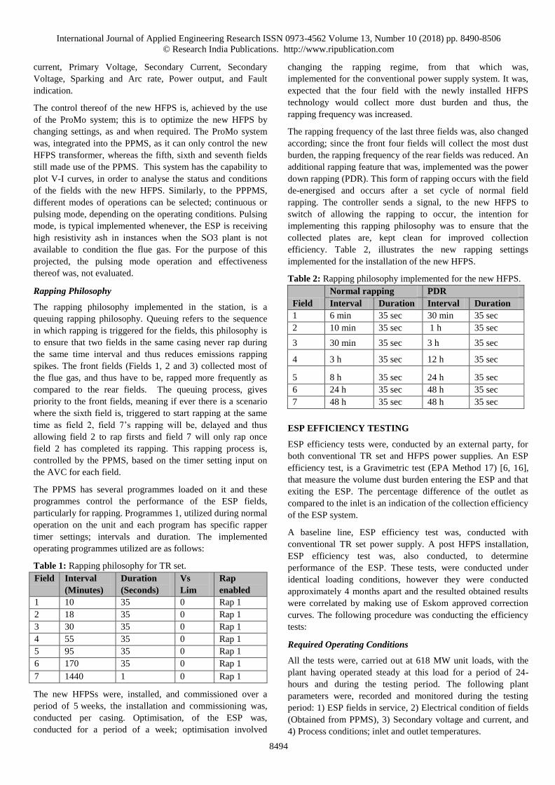
Rapping Philosophy

The rapping philosophy implemented in the station, is a

queuing rapping philosophy. Queuing refers to the sequence

in which rapping is triggered for the fields, this philosophy is

to ensure that two fields in the same casing never rap during

the same time interval and thus reduces emissions rapping

spikes. The front fields (Fields 1, 2 and 3) collected most of

the flue gas, and thus have to be, rapped more frequently as

compared to the rear fields. The queuing process, gives

priority to the front fields, meaning if ever there is a scenario

where the sixth field is, triggered to start rapping at the same

time as field 2, field 7’s rapping will be, delayed and thus

allowing field 2 to rap firsts and field 7 will only rap once

field 2 has completed its rapping. This rapping process is,

controlled by the PPMS, based on the timer setting input on

the AVC for each field.

The PPMS has several programmes loaded on it and these

programmes control the performance of the ESP fields,

particularly for rapping. Programmes 1, utilized during normal

operation on the unit and each program has specific rapper

timer settings; intervals and duration. The implemented

operating programmes utilized are as follows:

Table 1: Rapping philosophy for TR set.

Field Interval

(Minutes)

Duration

(Seconds)

Vs

Lim

Rap

enabled

1 10 35 0 Rap 1

2 18 35 0 Rap 1

3 30 35 0 Rap 1

4 55 35 0 Rap 1

5 95 35 0 Rap 1

6 170 35 0 Rap 1

7 1440 1 0 Rap 1

The new HFPSs were, installed, and commissioned over a

period of 5 weeks, the installation and commissioning was,

conducted per casing. Optimisation, of the ESP was,

conducted for a period of a week; optimisation involved

changing the rapping regime, from that which was,

implemented for the conventional power supply system. It was,

expected that the four field with the newly installed HFPS

technology would collect more dust burden and thus, the

rapping frequency was increased.

The rapping frequency of the last three fields was, also changed

according; since the front four fields will collect the most dust

burden, the rapping frequency of the rear fields was reduced. An

additional rapping feature that was, implemented was the power

down rapping (PDR). This form of rapping occurs with the field

de-energised and occurs after a set cycle of normal field

rapping. The controller sends a signal, to the new HFPS to

switch of allowing the rapping to occur, the intention for

implementing this rapping philosophy was to ensure that the

collected plates are, kept clean for improved collection

efficiency. Table 2, illustrates the new rapping settings

implemented for the installation of the new HFPS.

Table 2: Rapping philosophy implemented for the new HFPS.

Field

Normal rapping PDR

Interval Duration Interval Duration

1 6 min 35 sec 30 min 35 sec

2 10 min 35 sec 1 h 35 sec

3 30 min 35 sec 3 h 35 sec

4 3 h 35 sec 12 h 35 sec

5 8 h 35 sec 24 h 35 sec

6 24 h 35 sec 48 h 35 sec

7 48 h 35 sec 48 h 35 sec

ESP EFFICIENCY TESTING

ESP efficiency tests were, conducted by an external party, for

both conventional TR set and HFPS power supplies. An ESP

efficiency test, is a Gravimetric test (EPA Method 17) [6, 16],

that measure the volume dust burden entering the ESP and that

exiting the ESP. The percentage difference of the outlet as

compared to the inlet is an indication of the collection efficiency

of the ESP system.

A baseline line, ESP efficiency test was, conducted with

conventional TR set power supply. A post HFPS installation,

ESP efficiency test was, also conducted, to determine

performance of the ESP. These tests, were conducted under

identical loading conditions, however they were conducted

approximately 4 months apart and the resulted obtained results

were correlated by making use of Eskom approved correction

curves. The following procedure was conducting the efficiency

tests:

Required Operating Conditions

All the tests were, carried out at 618 MW unit loads, with the

plant having operated steady at this load for a period of 24-

hours and during the testing period. The following plant

parameters were, recorded and monitored during the testing

period: 1) ESP fields in service, 2) Electrical condition of fields

(Obtained from PPMS), 3) Secondary voltage and current, and

4) Process conditions; inlet and outlet temperatures.



8495

Isokinetic dust sampling

Five isokinetic tests were, carried out at each duct; with each

inlet duct being equipped with four sampling ports and the

outlet duct having six sampling ports. Four sets of sampling

equipment were used simultaneously and placed so that two

casings are, traversed sequentially by one set of equipment

[16]. An effort was, made to start and stop the isokinetic

sampling simultaneously on all casings, more especially the

corresponding inlet and outlet positions on a specific ESP

Casing. A probe was, inserted to the deepest point in the

traverse where sampling started.

The traversing started simultaneously on the RH Outer and

LH Inner and progressed to the RH Inner and LH Outer. The

obtained data was, captured for each ducting, analysed and

averaged out to determine the combine collection efficiency of

the ESP. These results will be the bases of determining and

quantifying the exact reduction or lack thereof, in the ESP as,

a result of implementing two types of power supply

technologies.

ESP EFFICIENCY TEST RESULTS

The ESP performance test was, conducted for both power

supply technologies; the test mainly focuses on the process

parameters, in terms of flue gas volume flow in and out of the

ESP and other process conditions such as coal quality.

Isometric sampling was, conducted on the inlet and outlet duct

of the ESP casings, these representative samples are, used to

determine the collection efficiency of the ESP. Particulate

emission measurements were, carried out employing

procedures and equipment that comply with the requirements

of EN 13284-1 [17], [19]. The VDI correlation procedure was,

followed in the determination of the linear regression of the

correlation spot check. The baseline ESP efficiency test was,

conducted with conventional TR sets installed and thereafter,

a second efficiency test was, conducted with the new HFPS

installed.

Baseline ESP efficiency test with TR set

Five ESP efficiency tests were, conducted on the unit, while

operating at full load of 618 MW generated load. Table 3,

illustrates the obtained results from the isometric testing

conducted during the ESP efficiency test. The average

efficiency of the ESP post outage and with conventional TR

sets was, found to be 97.1%; emitting at 42.8 mg/Nm3, at an

average boiler load of 619 MW.

Table 3: Isometric ESP efficiency test results.

Post HFPS installation ESP efficiency test

The ESP efficiency test was, subsequently performed after the

optimisation process had, been completed. Table 4, gives the

obtained results for the efficiency test conducted with the new

HFPS installed, on the first four fields of the ESP casings. The

emissions were, found to be 19.3 mg/Nm3 and were, maintained

at this level consistently.

Table 4: ESP efficiency test results post HFPS installation.

It can, be, seen from table 4, that the ESP was experiencing

higher flue gas volume flows, as compared to those measured

on the baseline efficiency test. For the post, HFPS installation

efficiency test the volume flow have increased by up to 21% on

some casings and the dust concentration have increased by up to

22% on some of the casings. However, despite these increases

in the process conditions, the obtained emissions were less that

those obtained in the baseline tests, giving a 45% emissions

reduction from baseline.

Electrical performance for both technologies

A field by field electrical performance was conducted for the

front four fields. The electrical performance was taken post

outage for the conventional TR sets and subsequently post

optimization of the new HFPS. The voltage and current

measurements were taken for an hour’s operation during the

ESP efficiency test.

The electrical performance comparison was, conducted for each

of the first four fields; for the operation of a conventional TR set

and that of a HFPS transformer. The analysis focuses on the

power input delivered into the field, as well as the ripple effect

contained in voltage delivered into the fields. The presented

electrical waveforms were taken from the plant historian, which

records the measured plant operating parameters in accordance

to the Metering and Measurement Systems for Power Stations

in Generation Standard; 240-563590.

The graphs shown data collected during the ESP efficiency test

for each power supply technology. The data is sampled at every

30 seconds and averaged out to give an hourly average, which

was used to plot the electrical performance. The unit was at a

fixed load of 618 MW, for both instance when data was

captured.

Table 5, illustrates the collected electrical data during the

process of conducting the ESP efficiency tests. The data was

taken for a period of 24 hours; from midnight to midnight. The

data was put in the same table although the two overall ESP

efficiency tests were conducted 3 months apart.

Test no.Boiler

Load

% of Total

Air flow

Standard

Deviation (%

of Total air

flow)

Effective

emissions

Dust

Concentration

Average

isokineticity

average O2

Concerntration

at ESP inlet

MW kg/s % -mg/Nm^3 at

10% O2% mm

1 618.8 580.6 1.4 73.7 30.3 97.8 4.8

2 619.2 572.7 1.2 34.3 18.1 98.2 4.3

3 618.9 581.4 1.1 40.5 19.2 95.9 4.4

4 619.1 573.6 1.0 32.0 22.9 96.7 4.5

5 619.2 575.1 1.1 33.7 15.4 96.8 4.6

Average 619.0 576.7 1.2 42.8 21.2 97.1 4.5

Test no.Boiler

Load

% of Total

Air flow

Standard

Deviation (%

of Total air

flow)

Effective

emissions

Dust

Concentration

Average

isokineticity

average O2

Concerntration

at ESP inlet

MW kg/s % -mg/Nm^3 at

10% O2% mm

1 618.2 594.7 1.1 19.3 36.5 95.0 7.1

2 619.5 598.2 1.1 20.3 28.9 96.1 6.8

3 618.6 599.0 1.0 24.0 34.4 95.4 6.8

4 619.6 579.4 1.1 13.8 7.3 98.1 6.2

5 619.7 587.9 0.6 19.1 17.7 98.4 7.1

Average 619.1 591.8 1.0 19.3 25.0 96.6 6.8



8496

Table 5: LHO 1 current and voltage measurement during the

ESP efficiency tests for TR set and the new HFPS.

Figure 6 illustrates the difference in electrical performance of

the LHO 1 field, when supplied by a TR set and when

supplied by an HFPS.

Figure 6: LHO 1 electrical performance for TR set and HFPS.

It can be seen from figure 6, that the electrical performance of

LHO 1 field increased significantly. The current input into the

field went from below 300 mA for a TR set and could be

maintained above 600 mA twice that which the TR set was

able to supply. The voltage also increase from low 40 kV for a

TR set, to above 40 kV, with the highest voltage being 48 kV

supplied by a HFPS. This was a drastic improvement seen on

the first field, with consideration that no mechanical repairs

were conducted internal from when both measurements were

conducted. Table 6 illustrates the collected electrical data

during the process of conducting the ESP efficiency tests.



The current and voltage measurement as presented in table 6 are

for both power supply technologies. The data was used to plot

the electrical performance of the LHO 2 field; as seen on figure

7.


The electrical performance of the LHO 2 field saw an

improvement in the current and voltage, when the HFPS was

installed in place of TR set. The TR set was able to supply and

maintain a current of about 900 mA, however with the HFPS

was able to produce current above 1600 mA. The voltage input

into the field did not change drastically, although the TR set was

Time

TR Set -

LHO 1 Is

TR Set

LHO 1 Vs

HFPS-

LHO 1 Is

HFPS-

LHO 1 Vs

00:00 - 01:00 283.55 26.45 929.68 39.72

01:00 - 02:00 102.28 39.67 1291.92 46.97

02:00 - 03:00 81.02 40.22 1288.32 48.08

03:00 - 04:00 96.50 41.38 1227.78 47.58

04:00 - 05:00 97.93 41.58 890.95 45.81

05:00 - 06:00 96.22 41.47 892.33 45.83

06:00 - 07:00 115.07 41.88 455.28 31.50

07:00 - 08:00 92.77 40.83 15.35 14.41

08:00 - 09:00 104.63 42.03 949.97 43.20

09:00 - 10:00 99.12 40.95 983.25 45.76

10:00 - 11:00 75.90 38.33 858.48 44.93

11:00 - 12:00 69.65 38.52 927.92 45.47

12:00 - 13:00 76.40 38.82 1031.70 48.61

13:00 - 14:00 88.87 39.77 1068.35 46.43

14:00 - 15:00 70.93 38.60 1052.17 48.52

15:00 - 16:00 79.45 39.60 790.88 43.79

16:00 - 17:00 98.78 41.70 850.22 45.05

17:00 - 18:00 95.22 40.55 631.03 39.76

18:00 - 19:00 100.98 39.27 15.83 13.45

19:00 - 20:00 89.10 40.25 20.88 16.17

20:00 - 21:00 116.57 41.03 16.87 15.26

21:00 - 22:00 105.47 41.52 23.65 15.99

22:00 - 23:00 115.93 42.52 21.57 17.30

23:00 - 00:00 137.52 43.28 24.77 17.02

LHO 1

Time

TR Set

LHO 2 Is

TR Set

LHO 2 Vs

HFPS-

LHO 2 Is

HFPS-

LHO 2 Vs

00:00 - 01:00 625.03 33.88 1585.60 40.92

01:00 - 02:00 963.75 46.65 1672.37 42.75

02:00 - 03:00 955.55 47.38 1667.87 42.67

03:00 - 04:00 976.98 47.52 1642.47 42.30

04:00 - 05:00 1004.50 47.12 1625.73 43.64

05:00 - 06:00 919.13 47.65 1625.73 43.64

06:00 - 07:00 819.90 46.50 1539.40 46.21

07:00 - 08:00 914.23 47.20 1403.23 48.06

08:00 - 09:00 957.87 48.08 1675.82 44.82

09:00 - 10:00 931.30 47.53 1636.65 43.10

10:00 - 11:00 792.73 46.93 1665.83 44.49

11:00 - 12:00 731.53 45.98 1629.48 43.83

12:00 - 13:00 693.35 46.35 1642.83 43.79

13:00 - 14:00 737.95 46.20 1644.15 43.35

14:00 - 15:00 665.92 46.82 1640.50 42.90

15:00 - 16:00 678.77 46.40 1647.78 45.60

16:00 - 17:00 614.22 44.98 1636.32 45.78

17:00 - 18:00 580.15 45.43 1471.87 46.14

18:00 - 19:00 626.52 45.37 794.10 46.20

19:00 - 20:00 583.88 45.55 920.70 45.45

20:00 - 21:00 753.08 45.50 1035.22 46.78

21:00 - 22:00 748.55 46.10 1301.20 48.61

22:00 - 23:00 755.73 46.10 1113.18 47.42

23:00 - 00:00 800.33 47.18 1071.32 47.39

LHO 2



8497

producing a little more voltage as compared to the HFPS.



Table 7 illustrates the collected electrical data during the

process of conducting the ESP efficiency tests.


Figure 8 represent a graphical plot of the LHO 3 electrical

performance for both TR set and HFP. The only significant

difference that was noted from the two supply technologies

was that the HFPS was able to input a high voltage into the

field than that of the TR set. The HFPS was able to maintain a

voltage of above 47 kV, whereas the TR set could only

maintain voltage a low 30 kV. The current input into the field

for both transformers was at maximum. The higher voltage,

from the HFPS increases the electric field strength for the

capturing of the charged dust particles.



Table 8 illustrates the collected electrical data for LHO 4 during

the process of conducting the ESP efficiency tests. The LHO 4’s

electrical performance is, illustrated on figure 9; as per data

presented on table 8.


The LHO 4’s electrical performance improved significantly

with the installation of the HFPS. The current input into the ESP

field increased from around 400 mA to full rated input current

of 1600 mA. The voltage input into the field also increase from

around 48 kV to 53 kV.

Time

TR Set

LHO 3 Is

TR Set

LHO 3 Vs

HFPS-

LHO 3 Is

HFPS-

LHO 3 Vs

00:00 - 01:00 1110.50 20.87 1555.85 47.18

01:00 - 02:00 1659.88 31.82 1698.92 48.46

02:00 - 03:00 1654.35 31.90 1690.50 47.66

03:00 - 04:00 1655.33 31.82 1671.05 46.35

04:00 - 05:00 1645.63 31.70 1678.07 46.67

05:00 - 06:00 1667.40 31.93 1678.08 46.67

06:00 - 07:00 1661.70 32.45 1650.28 46.38

07:00 - 08:00 1691.63 32.17 1623.05 47.54

08:00 - 09:00 1625.50 31.60 1642.88 46.26

09:00 - 10:00 1702.77 32.02 1699.52 46.81

10:00 - 11:00 1656.98 31.85 1686.88 46.41

11:00 - 12:00 1674.73 31.93 1646.13 45.92

12:00 - 13:00 1645.87 31.83 1670.73 46.34

13:00 - 14:00 1646.75 31.77 1655.83 46.01

14:00 - 15:00 1651.70 31.98 1670.95 45.89

15:00 - 16:00 1532.15 31.85 1697.13 46.92

16:00 - 17:00 1452.08 31.90 1685.03 47.18

17:00 - 18:00 1283.38 32.15 1639.25 46.34

18:00 - 19:00 1432.37 33.08 1558.42 49.48

19:00 - 20:00 1322.60 32.90 1427.40 49.50

20:00 - 21:00 1418.30 32.93 1323.13 49.54

21:00 - 22:00 1590.50 32.52 1556.83 49.77

22:00 - 23:00 1535.72 32.35 1521.00 49.51

23:00 - 00:00 1544.75 32.57 1568.50 50.87

LHO 3

Time

TR Set

LHO 4 Is

TR Set

LHO 4 Vs

HFPS-

LHO 4 Is

HFPS-

LHO 4 Vs

00:00 - 01:00 413.12 31.37 1179.27 47.31

01:00 - 02:00 471.22 47.52 1472.15 52.89

02:00 - 03:00 455.52 46.87 1535.22 52.52

03:00 - 04:00 458.73 47.35 1636.83 53.28

04:00 - 05:00 460.37 46.98 1668.25 53.11

05:00 - 06:00 462.22 47.28 1668.25 53.10

06:00 - 07:00 482.37 48.40 1679.45 53.45

07:00 - 08:00 483.78 48.08 1649.52 52.74

08:00 - 09:00 474.43 47.80 1655.88 53.52

09:00 - 10:00 487.07 48.23 1642.02 52.08

10:00 - 11:00 485.35 48.93 1671.10 52.87

11:00 - 12:00 434.08 46.23 1671.10 52.92

12:00 - 13:00 409.07 46.48 1683.03 53.77

13:00 - 14:00 405.20 46.67 1645.32 52.76

14:00 - 15:00 357.73 45.47 1668.93 53.08

15:00 - 16:00 385.72 46.00 1655.90 52.53

16:00 - 17:00 389.45 46.53 1627.23 51.88

17:00 - 18:00 393.50 46.55 1673.17 53.14

18:00 - 19:00 413.08 47.32 1536.95 50.89

19:00 - 20:00 416.63 46.80 1470.83 51.26

20:00 - 21:00 422.10 47.05 1361.72 50.89

21:00 - 22:00 407.08 46.45 1567.82 52.60

22:00 - 23:00 440.37 48.15 1543.58 52.20

23:00 - 00:00 392.26 47.36 1571.73 52.65

LHO 4



8498

Table 9: LHI 1 current and voltage measurement during the


Table 9 presents the electrical measurements for the LHI 1’s

performance. It is noted that at around 17:00, the TR sets

reading went to zero, which indicates that the field had tripped

at this stage.

Figure 10: LHI 1 electrical performance for TR set and

HFPS.

The installation on the HFPS on the LHI 1 did not result in an

improved electrical performance although the current was not

stable. Due to excessive sparking, probably caused by a loose

discharge electrode wire.




performance. LHI 2’s electrical performance is presented on

figure 11, plotted from data acquired from table 10.

Figure 11: LHI 2 electrical performance for TR set and HFPS.

The LHI 2’s performance was similar to that observed on LHI

1. The field was sparking excessively, thus not allowing stable

operating conditions. The TR set was able to maintain

consistent current as the controller allows for manual

intervention and can be set to a point where it can operate

without frequent trips due to sparking and arcing.

TR Set

LHI 1 Is

TR Set

LHI 1 Vs

HFPS-LHI

1 Is

HFPS-LHI

1 Vs

00:00 - 01:00 112.57 37.87 1521.53 42.07

01:00 - 02:00 188.88 55.18 1588.55 44.27

02:00 - 03:00 203.73 53.87 1576.48 44.45

03:00 - 04:00 195.95 53.93 1462.47 43.77

04:00 - 05:00 192.93 53.77 588.53 42.13

05:00 - 06:00 189.20 55.05 577.75 42.09

06:00 - 07:00 198.18 54.17 366.45 39.20

07:00 - 08:00 210.83 55.72 305.73 38.34

08:00 - 09:00 236.52 54.90 747.92 41.24

09:00 - 10:00 241.58 54.97 682.05 41.29

10:00 - 11:00 247.75 53.52 845.25 42.81

11:00 - 12:00 245.62 52.65 628.42 42.47

12:00 - 13:00 252.37 52.37 754.42 40.98

13:00 - 14:00 216.43 54.35 1225.30 44.70

14:00 - 15:00 249.57 52.23 1093.48 42.69

15:00 - 16:00 221.98 52.10 654.68 40.94

16:00 - 17:00 30.87 2.03 611.18 41.21

17:00 - 18:00 0.00 0.00 419.38 39.77

18:00 - 19:00 0.00 0.00 209.07 36.94

19:00 - 20:00 0.00 0.00 208.63 37.29

20:00 - 21:00 0.00 0.00 238.30 37.14

21:00 - 22:00 0.00 0.00 336.37 40.34

22:00 - 23:00 0.00 0.00 266.08 37.94

23:00 - 00:00 0.00 0.00 265.85 38.83

LHI 1TR Set

LHI 2 Is

TR Set

LHI 2 Vs

HFPS-LHI

2 Is

HFPS-LHI

2 Vs

00:00 - 01:00 206.10 20.73 1469.27 47.32

01:00 - 02:00 277.35 29.12 1614.40 49.24

02:00 - 03:00 274.12 30.28 1647.32 49.64

03:00 - 04:00 249.15 31.48 1653.02 50.26

04:00 - 05:00 241.07 30.52 1342.00 50.08

05:00 - 06:00 267.00 30.30 1336.98 50.08

06:00 - 07:00 256.93 30.52 823.38 47.95

07:00 - 08:00 263.83 30.12 450.97 45.50

08:00 - 09:00 281.15 31.57 1028.68 49.54

09:00 - 10:00 262.20 31.55 1213.70 50.49

10:00 - 11:00 278.52 31.48 1232.10 49.57

11:00 - 12:00 244.22 30.67 1171.17 49.05

12:00 - 13:00 224.48 30.07 1152.22 49.00

13:00 - 14:00 204.33 30.40 1480.20 49.68

14:00 - 15:00 185.38 31.07 1494.90 49.36

15:00 - 16:00 217.15 31.25 1098.67 47.88

16:00 - 17:00 170.02 29.45 923.10 48.13

17:00 - 18:00 217.63 29.58 678.33 47.40

18:00 - 19:00 248.85 30.82 245.02 42.51

19:00 - 20:00 269.32 30.82 257.27 42.83

20:00 - 21:00 286.85 30.28 278.17 43.10

21:00 - 22:00 290.20 31.00 447.43 46.62

22:00 - 23:00 299.03 29.80 353.35 45.36

23:00 - 00:00 283.87 30.05 325.88 45.17

LHI 2



8499




performance.

Figure 12: LHI 3 electrical performance for TR set and

HFPS.

Figure 12 presents the electrical performance of the LHI 3’s

field. Similar to that of LHI 1 and 2, this field was also

experiencing a high spark rate. The HFPS was still able to

maintain a higher electrical performance than that of the TR

set, in these upset conditions.




performance. It is noted the performance decreased after 17:00.

Figure 13 presents the performance of the LHI 4 as illustrated

by the value of table 12.

Figure 13: LHI 4 electrical performance for TR set and HFPS.

Similarly to all the other fields discussed, the installation of the

HFPS resulted in improved electrical performance. Although

this casing was experiencing excessive sparking, the HFPSs

were able to maintain a high electrical performance than that

which was possible with the TR sets.

TR Set

LHI 3 Is

TR Set

LHI 3 Vs

HFPS-LHI

3 Is

HFPS-LHI

3 Vs

00:00 - 01:00 133.12 25.35 976.08 45.22

01:00 - 02:00 106.03 37.77 1461.02 48.82

02:00 - 03:00 83.43 38.38 1588.62 49.36

03:00 - 04:00 74.73 39.43 1661.70 49.54

04:00 - 05:00 86.23 38.90 1518.82 47.78

05:00 - 06:00 78.15 39.22 1544.50 48.47

06:00 - 07:00 89.07 39.32 1085.60 46.08

07:00 - 08:00 78.13 38.27 512.97 42.56

08:00 - 09:00 81.65 38.72 922.45 46.19

09:00 - 10:00 99.50 39.18 1188.33 47.22

10:00 - 11:00 94.35 39.63 1239.40 46.81

11:00 - 12:00 103.73 40.03 1141.73 45.93

12:00 - 13:00 70.37 38.20 1154.38 46.75

13:00 - 14:00 70.05 39.30 1390.77 47.66

14:00 - 15:00 50.67 37.47 1554.23 48.67

15:00 - 16:00 51.03 38.20 1230.05 46.50

16:00 - 17:00 31.93 37.22 930.72 44.72

17:00 - 18:00 29.93 37.50 737.08 43.95

18:00 - 19:00 37.75 38.02 200.40 39.56

19:00 - 20:00 42.03 38.97 168.37 39.17

20:00 - 21:00 47.20 38.45 161.68 39.05

21:00 - 22:00 47.45 39.38 300.50 43.28

22:00 - 23:00 51.22 39.42 208.97 42.27

23:00 - 00:00 53.21 38.97 200.72 41.77

LHI 3

TR Set

LHI 4 Is

TR Set

LHI 4 Vs

HFPS-LHI

4 Is

HFPS-LHI

4 Vs

00:00 - 01:00 312.80 47.90 863.23 43.64

01:00 - 02:00 265.97 46.50 1356.82 47.99

02:00 - 03:00 373.50 47.07 1547.48 48.09

03:00 - 04:00 387.47 46.93 1647.63 48.36

04:00 - 05:00 350.93 47.20 1655.32 48.23

05:00 - 06:00 367.82 47.33 1655.33 48.23

06:00 - 07:00 360.53 47.28 1489.15 47.19

07:00 - 08:00 350.32 46.68 1042.40 45.72

08:00 - 09:00 379.12 47.28 1198.05 46.05

09:00 - 10:00 376.98 47.43 1517.92 47.70

10:00 - 11:00 356.15 46.53 1565.90 47.39

11:00 - 12:00 314.50 46.20 1607.87 48.24

12:00 - 13:00 254.43 44.55 1605.03 48.22

13:00 - 14:00 262.65 45.88 1636.20 47.54

14:00 - 15:00 244.80 46.57 1664.87 47.65

15:00 - 16:00 249.93 46.78 1541.83 46.70

16:00 - 17:00 144.67 47.77 1396.33 46.43

17:00 - 18:00 138.23 47.75 1226.12 45.40

18:00 - 19:00 174.97 47.17 521.98 43.16

19:00 - 20:00 189.20 47.33 312.25 41.03

20:00 - 21:00 191.10 48.00 279.85 42.21

21:00 - 22:00 179.20 46.85 419.53 43.03

22:00 - 23:00 200.68 48.33 387.60 42.74

23:00 - 00:00 176.00 47.51 365.08 43.23

LHI 4



8500

Table 13: RHI 1 current and voltage measurement during the


Table 13, represents the electrical data for the RHI 1’s

performance.

Figure 14: RHI 1 electrical performance for TR set and

HFPS.

The RHI 1’s electrical performance is plotted on figure 14.

The TR set’s performance for this field is typical of how low

the electrical performance of the TR set can be more

especially for the first field. The current input into the field

was consistently below 350 mA with the TR set in operation.

The installation of the HFPS saw the current input into the

field increase to above 1000 mA. The voltage of the TR set

was slightly above that which the HFPS could manage,

however due to the inability to produce a high enough current;

the high voltage has not significant influence on the collection

of dust burden.



Electrical performance of the RHI 2 field is shown on table 14.

Figure 15: RHI 2 electrical performance for TR set and HFPS.

Figure 15, presented the graphical representation of the data on

table 14. It is noted that the electrical performance of the HFPS

surpassed that of the TR set, with the HFPS being able to input

full load current into the field. The TR sets voltage is

significantly higher than that of the of the HFPS, reason being

the controller algorithm is such that was force the TR set to

push the voltage as high as possible in order to achieved the

desired 1600 mA. Since the HFPS is able to achieve full load

operational current, at a lower voltage, it simple maintains the

voltage level at which the full load current was achieved.

TR Set

RHI 1 Is

TR Set

RHI 1 Vs

HFPS-RHI

1 Is

HFPS-RHI

1 Vs

00:00 - 01:00 426.52 34.97 1551.43 43.32

01:00 - 02:00 330.12 48.53 1647.20 46.50

02:00 - 03:00 370.23 50.82 1670.73 47.11

03:00 - 04:00 381.17 51.68 1631.80 46.11

04:00 - 05:00 343.73 51.68 1620.67 47.60

05:00 - 06:00 340.85 51.45 1618.08 47.63

06:00 - 07:00 324.25 51.57 1348.98 46.24

07:00 - 08:00 315.50 51.98 1080.42 45.44

08:00 - 09:00 325.93 51.78 1527.73 48.04

09:00 - 10:00 315.38 51.32 1327.35 45.94

10:00 - 11:00 311.13 50.90 1225.52 45.77

11:00 - 12:00 280.07 50.95 1521.20 47.85

12:00 - 13:00 306.80 52.47 1548.15 48.20

13:00 - 14:00 287.72 50.93 1582.92 45.33

14:00 - 15:00 265.85 50.65 1617.57 46.59

15:00 - 16:00 276.00 51.18 1634.65 46.66

16:00 - 17:00 293.62 50.32 1606.02 46.95

17:00 - 18:00 308.37 49.55 1416.68 46.66

18:00 - 19:00 313.90 49.97 828.20 43.46

19:00 - 20:00 289.07 49.98 931.95 42.96

20:00 - 21:00 311.80 48.27 960.98 44.18

21:00 - 22:00 335.70 51.22 913.72 44.06

22:00 - 23:00 329.68 49.70 1085.30 43.70

23:00 - 00:00 320.10 51.16 1120.83 44.56

RHI 1

TR Set

RHI 2 Is

TR Set

RHI 2 Vs

HFPS-RHI

2 Is

HFPS-RHI

2 Vs

00:00 - 01:00 188.07 56.45 1567.45 43.40

01:00 - 02:00 272.15 56.37 1638.30 43.84

02:00 - 03:00 244.50 56.63 1671.55 44.81

03:00 - 04:00 207.82 56.67 1652.80 44.13

04:00 - 05:00 180.38 56.37 1605.73 43.52

05:00 - 06:00 164.28 55.60 1634.05 44.22

06:00 - 07:00 185.85 56.57 1631.70 45.80

07:00 - 08:00 212.20 57.03 1574.23 46.10

08:00 - 09:00 185.28 57.17 1620.02 46.09

09:00 - 10:00 174.87 56.85 1618.40 46.79

10:00 - 11:00 157.25 56.00 1601.98 46.28

11:00 - 12:00 143.80 56.22 1644.55 46.96

12:00 - 13:00 175.48 56.58 1644.10 46.79

13:00 - 14:00 145.05 56.02 1647.48 46.70

14:00 - 15:00 167.63 56.72 1629.02 45.23

15:00 - 16:00 182.40 57.02 1652.58 45.88

16:00 - 17:00 187.70 56.40 1627.35 45.85

17:00 - 18:00 172.12 56.28 1601.47 46.44

18:00 - 19:00 168.17 55.20 1524.87 47.06

19:00 - 20:00 159.57 55.50 1497.87 46.79

20:00 - 21:00 158.90 55.53 1564.35 47.33

21:00 - 22:00 202.30 56.90 1522.85 47.51

22:00 - 23:00 294.77 56.35 1584.85 47.65

23:00 - 00:00 347.46 58.33 1562.45 46.54

RHI 2



8501



Table 15, illustrates the electrical performance data of the RHI

3 field.

Figure 16: RHI 3 electrical performance for TR set and

HFPS.

RHI 3’s electrical performance is plotted on figure 16, it is

noted that with the TR set in operation, the input current was

significantly low. The installation of the HFPS resulted in

maximum input current being fed into the field and

maintained.



Table 16, illustrates the electrical performance data of the RHI 4

field. The RHI 4’s electrical performance was not stable for

both power supply technologies, as seen on figure 17.

Figure 17: RHI 4 electrical performance for TR set and HFPS.

The performance of the field was within specification for both

power supply technologies, although the field was experiencing

excessive sparking resulting frequent performance dips.

TR Set

RHI 3 Is

TR Set

RHI 3 Vs

HFPS-RHI

3 Is

HFPS-RHI

3 Vs

00:00 - 01:00 497.53 30.28 1652.45 43.98

01:00 - 02:00 616.63 42.27 1699.62 43.90

02:00 - 03:00 601.13 39.93 1643.02 42.36

03:00 - 04:00 572.45 40.05 1642.93 42.12

04:00 - 05:00 600.87 40.62 1642.88 42.38

05:00 - 06:00 629.07 40.90 1642.88 42.37

06:00 - 07:00 651.32 41.32 1696.70 43.90

07:00 - 08:00 724.08 42.33 1642.95 42.91

08:00 - 09:00 582.30 39.87 1671.18 43.88

09:00 - 10:00 577.13 39.88 1657.50 44.04

10:00 - 11:00 602.97 40.10 1669.70 44.30

11:00 - 12:00 619.62 41.58 1690.92 44.81

12:00 - 13:00 680.00 42.17 1642.98 43.81

13:00 - 14:00 610.43 41.72 1659.72 44.20

14:00 - 15:00 690.20 42.88 1671.17 43.94

15:00 - 16:00 698.00 43.55 1699.42 44.67

16:00 - 17:00 697.10 43.02 1642.78 43.33

17:00 - 18:00 718.33 43.82 1670.87 44.33

18:00 - 19:00 657.18 43.35 1642.35 44.12

19:00 - 20:00 651.42 42.68 1670.20 44.70

20:00 - 21:00 677.65 43.17 1642.73 44.04

21:00 - 22:00 707.18 43.98 1671.17 44.83

22:00 - 23:00 672.95 42.72 1639.28 44.29

23:00 - 00:00 704.13 43.05 1668.98 45.08

RHI 3 TR Set

RHI 4 Is

TR Set

RHI 4 Vs

HFPS-RHI

4 Is

HFPS-RHI

4 Vs

00:00 - 01:00 1309.22 39.12 1646.52 41.85

01:00 - 02:00 1618.05 47.18 1405.00 39.55

02:00 - 03:00 392.73 32.90 1636.85 41.71

03:00 - 04:00 1429.43 45.58 1635.08 41.12

04:00 - 05:00 1604.32 47.98 1668.53 41.34

05:00 - 06:00 1552.65 47.67 1668.55 41.35

06:00 - 07:00 1619.13 48.85 1365.77 39.34

07:00 - 08:00 1691.33 49.30 1620.80 41.52

08:00 - 09:00 1174.08 43.02 1671.65 42.68

09:00 - 10:00 615.10 36.02 1351.88 39.59

10:00 - 11:00 1657.02 49.33 1635.70 42.25

11:00 - 12:00 1579.98 47.88 1357.00 39.69

12:00 - 13:00 1635.52 49.20 1629.92 42.23

13:00 - 14:00 1649.02 49.50 1679.05 42.86

14:00 - 15:00 1590.63 48.82 1643.93 41.86

15:00 - 16:00 353.52 34.85 1323.10 39.25

16:00 - 17:00 1396.00 46.75 1674.47 42.83

17:00 - 18:00 1510.62 47.52 1640.17 42.13

18:00 - 19:00 1574.63 49.22 1506.48 40.75

19:00 - 20:00 1533.65 48.87 1430.17 40.11

20:00 - 21:00 1464.58 47.87 1697.60 43.18

21:00 - 22:00 1186.13 45.73 1614.52 41.71

22:00 - 23:00 747.35 41.38 1339.58 39.82

23:00 - 00:00 1559.51 48.85 1638.25 42.34

RHI 4



8502

Table 17: RHO 1 current and voltage measurement during the


Table 17, illustrates the electrical performance data of the

RHO 1 field. It was noted that by the time the HFPS was

installed, that field had an internal fault, which was

subsequently repaired during an opportunity.

Figure 18: RHO 1 electrical performance for TR set and

HFPS.

Figure 18 illustrates the performance of the RHO 1 field,

unfortunately the field experienced an internal fault when the

HFPS was installed and thus its performance could not be

determined at the stage when the testing was conducted.



Table 18, illustrates the electrical performance data of the RHO

2 field. The performance of this field was within specification

for both power supply technologies. The TR set was able to

produce and maintain a current input of above 700 mA at a

voltage level of 57 kV, exceptional performance for a TR set

more especially that it is operating on the second field. The

installation of the HFPS further improved the electrical

performance of the field, with current exceeding a 1000 mA.

Figure 19 presents the plotted data as shown on table 18.

Figure 19: RHO 2 electrical performance for TR set and HFPS.

TR Set

RHO 1 Is

TR Set

RHO 1 Vs

HFPS-

RHO 1 Is

HFPS-

RHO 1 Vs

00:00 - 01:00 485.65 24.03 26.88 9.85

01:00 - 02:00 585.53 24.93 15.97 10.51

02:00 - 03:00 561.22 24.80 19.22 11.36

03:00 - 04:00 617.95 24.28 14.03 11.14

04:00 - 05:00 635.83 24.63 15.38 10.90

05:00 - 06:00 603.37 24.30 15.38 10.87

06:00 - 07:00 623.03 23.95 15.32 11.16

07:00 - 08:00 668.65 24.80 21.37 12.29

08:00 - 09:00 659.20 24.07 19.05 11.63

09:00 - 10:00 651.07 23.93 16.97 11.11

10:00 - 11:00 735.33 25.10 19.03 11.26

11:00 - 12:00 673.78 25.33 17.72 11.05

12:00 - 13:00 840.45 25.72 18.95 11.57

13:00 - 14:00 677.05 24.87 22.20 11.45

14:00 - 15:00 925.17 23.40 18.87 11.38

15:00 - 16:00 1404.03 25.57 19.47 11.46

16:00 - 17:00 1323.68 26.62 16.88 11.21

17:00 - 18:00 1179.75 27.17 16.08 11.40

18:00 - 19:00 1155.28 27.00 18.10 11.44

19:00 - 20:00 1224.40 27.75 18.20 11.33

20:00 - 21:00 1245.72 28.53 16.72 11.36

21:00 - 22:00 1181.37 28.37 14.02 9.96

22:00 - 23:00 1217.65 28.25 18.73 12.53

23:00 - 00:00 1193.89 27.97 14.00 10.51

RHO 1

TR Set

RHO 2 Is

TR Set

RHO 2 Vs

HFPS-

RHO 2 Is

HFPS-

RHO 2 Vs

00:00 - 01:00 287.13 34.80 1529.67 45.75

01:00 - 02:00 788.55 56.03 1634.95 48.59

02:00 - 03:00 807.60 56.85 1642.23 48.82

03:00 - 04:00 754.15 57.22 1626.78 49.05

04:00 - 05:00 740.37 57.27 1568.45 48.90

05:00 - 06:00 741.88 57.40 1565.50 48.87

06:00 - 07:00 707.23 55.72 1311.33 46.83

07:00 - 08:00 727.90 57.23 990.22 44.15

08:00 - 09:00 718.97 57.57 1044.18 44.13

09:00 - 10:00 692.75 57.25 1109.02 46.23

10:00 - 11:00 663.82 55.58 1311.63 46.04

11:00 - 12:00 652.43 55.53 1162.78 44.94

12:00 - 13:00 644.18 56.23 1100.32 44.99

13:00 - 14:00 584.63 53.77 1319.40 45.85

14:00 - 15:00 655.05 55.77 1378.70 45.82

15:00 - 16:00 664.02 56.03 1506.88 47.43

16:00 - 17:00 715.52 56.52 1557.13 47.36

17:00 - 18:00 720.35 56.38 1433.12 47.34

18:00 - 19:00 765.55 57.27 1200.15 45.88

19:00 - 20:00 746.07 57.00 1173.95 45.94

20:00 - 21:00 738.70 57.07 1106.00 44.97

21:00 - 22:00 745.47 56.57 1044.87 44.91

22:00 - 23:00 784.58 57.30 1150.53 46.27

23:00 - 00:00 740.03 56.41 1219.43 46.82

RHO 2



8503



Table 19, illustrates the electrical performance data of the

RHO 3 field. The TR set showed poor performance with, with

a current input into the field being below 200 mA, such poor

performance is typical due to internal fault condition such as a

defective rapping system. A shearing pin was replaced on the

discharge electrode rapping system and with the installation

on the HFPS, the input current into the field went to

maximum. Figure 20 shows the contrasting performances of

the two power supply systems.

Figure 20: RHO 3 electrical performance for TR set and

HFPS.



Table 20, illustrates the electrical performance data of the RHO

4 field. The RHO 4’s performance was within specification with

the TR set installed, as it was able to produce maximum current.

The installation of a HFPS result in the HFPS maintaining the

maximum current as well, however it managed to increase the

input voltage into the field as well. Figure 21, presents the

graphical plot of the data presented on table 20, for the

performance of the RHO 4 field.

Figure 21: RHO 4 electrical performance for TR set and HFPS.

The overall electrical performance of the two power supply

technologies has shown that the new HFPS have a, better

electrical conversion efficiency as compared to that of the TR

set. The LHO casing had a maximum power input of 228 kW,

TR Set

RHO 3 Is

TR Set

RHO 3 Vs

HFPS-

RHO 3 Is

HFPS-

RHO 3 Vs

00:00 - 01:00 424.88 20.72 1528.97 40.16

01:00 - 02:00 279.42 32.67 1660.88 42.58

02:00 - 03:00 221.15 32.08 1699.50 43.16

03:00 - 04:00 228.88 32.85 1642.48 41.61

04:00 - 05:00 227.42 32.98 1645.20 42.07

05:00 - 06:00 208.53 32.55 1645.22 42.08

06:00 - 07:00 204.32 32.83 1698.63 43.52

07:00 - 08:00 186.42 33.62 1641.25 43.14

08:00 - 09:00 179.73 32.93 1661.88 43.47

09:00 - 10:00 180.73 32.98 1636.35 42.92

10:00 - 11:00 165.62 33.08 1663.05 43.56

11:00 - 12:00 158.77 32.40 1661.12 43.65

12:00 - 13:00 155.83 32.08 1649.32 43.33

13:00 - 14:00 143.00 32.13 1648.33 43.04

14:00 - 15:00 169.88 34.93 1665.90 42.98

15:00 - 16:00 258.68 38.85 1649.60 42.77

16:00 - 17:00 292.80 38.30 1646.85 42.91

17:00 - 18:00 380.17 39.68 1669.48 43.15

18:00 - 19:00 396.23 39.58 1631.75 42.64

19:00 - 20:00 386.58 39.43 1641.15 42.43

20:00 - 21:00 379.28 38.90 1670.38 43.69

21:00 - 22:00 402.30 40.07 1683.55 44.05

22:00 - 23:00 379.90 40.53 1639.33 43.29

23:00 - 00:00 423.15 40.08 1695.53 43.97

RHO 3

TR Set

RHO 4 Is

TR Set

RHO 4 Vs

HFPS-

RHO 4 Is

HFPS-

RHO 4 Vs

00:00 - 01:00 768.27 21.97 1584.35 40.34

01:00 - 02:00 1642.20 34.53 1642.85 42.02

02:00 - 03:00 1652.28 34.68 1699.47 43.19

03:00 - 04:00 1665.53 34.87 1671.13 42.33

04:00 - 05:00 1707.78 35.18 1667.25 41.90

05:00 - 06:00 1665.07 34.98 1667.27 41.89

06:00 - 07:00 1675.15 35.78 1699.48 42.77

07:00 - 08:00 1632.97 35.47 1642.85 41.69

08:00 - 09:00 1690.55 35.92 1675.27 42.72

09:00 - 10:00 1666.40 35.75 1674.75 42.90

10:00 - 11:00 1669.43 35.70 1661.23 42.99

11:00 - 12:00 1698.65 35.23 1670.68 42.77

12:00 - 13:00 1619.53 34.85 1688.67 43.32

13:00 - 14:00 1443.42 33.98 1669.82 43.16

14:00 - 15:00 1600.03 35.23 1641.90 42.59

15:00 - 16:00 1669.95 35.72 1670.23 42.91

16:00 - 17:00 1602.93 35.48 1681.37 43.77

17:00 - 18:00 1607.60 35.83 1698.48 43.93

18:00 - 19:00 1694.03 36.28 1677.83 43.81

19:00 - 20:00 1678.10 36.25 1685.17 43.57

20:00 - 21:00 1590.17 36.08 1670.42 43.07

21:00 - 22:00 1655.37 36.15 1670.90 42.89

22:00 - 23:00 1628.87 36.25 1642.50 42.49

23:00 - 00:00 1635.57 36.31 1671.03 43.08

RHO 4



8504

with TR set in operation, whereas the new HFPS was able to

produce a maximum power input of 389 kW. This gave a

casing power input increase of 41%. The LHI casing had a

maximum power input of 237 kW, with TR set in operation,

whereas the new HFPS was able to produce a maximum

power input of 419 kW. This gave a casing power input

increase of 43%.

The RHI casing had a maximum power input of 253 kW, with

TR set in operation, whereas the new HFPS was able to

produce a maximum power input of 403 kW. This gave a

casing power input increase of 37%. The highest power input

into the RHO casing was 275 kW for conventional TR sets,

whereas the highest for a casing with new HFPS installed

went up to 420 kW.

This gave a casing power input increase of 35%. The overall

electrical performance increase of the ESP casings is,

expected to result in improved collection efficiency of the

ESP.

Emissions performance comparison

Figure 22 illustrates the emissions performance of the unit, it

can, be, seen how the emissions reduced and consistently

maintained at low levels.

The emissions recorded shows that for the period in which the

conventional TR sets were in operation the emissions were

low; however the inconsistency in the electrical performance

of the TR sets, resulted in a fluctuation of the emissions. At

the time, when all 16 new HFPS were installed and fully

operation, it could be seen that the emissions reduced and

were maintained, this is due to the consistency that the new

HFPS are able to maintain high electrical power input into the

ESP.

Figure 22: Emissions performance.

The ESP efficiency test showed that the ESP was emitting

42.8 mg/Nm3 with conventional TR sets installed, and

19.3 mg/Nm3 with new HFPS transformers installed in the front

four fields of all the casings. The reduction in emission was

45%, which is extremely significant. Particulate emissions are,

governed by the air quality legislation, which requires the

operation of a power station to comply with the stipulated

emissions limits at all times during operation.

Failure to comply with stipulated emissions limits as specified

by the legislation carries a stiff fine or even jail time. In order to

comply with the set out emissions limits, power stations have

resorted to taking load losses; reduction in boiler production

capacity in order to reduce particulate emissions. The practice

of taking load losses due to ineffective ESP performance is a

costly exercise, as the power station loses revenue for every

MW that is not generated. This chapter will discuss the exact

cost implications of operating with ineffective ESPs that result

in units having to take load losses in order to meet emissions

limits.

Cost of emissions

A power station that is, rated for 618 MW, full load production

is required to maintain emissions below 100 mg/Nm3, daily.

Thus, if a unit is unable to maintain emissions below

100 mg/Nm3, a 118 MW load loss is typically taken during of

peak periods. Off peak, periods are from 10:00 am to 17:00 pm

and 22:00 pm to 05:00. This means a unit can run on average 10

hours a day with a 118 MW load loss, which is equivalent to

1.2 GWhrs of power that is, not generated during that period.

That is 19% of the full load generating capacity that is lost, due

to high particulate emissions.

The national electricity supplier has been struggling to meet the

country’s electricity demand since early 2007. A reduction in

production is not ideal as it further puts pressure on the

organisation and increases the likelihood of load shedding

being, implemented in the country. The revenue loss because of

these load losses is also significant, as it limits the suppliers’

cash flow. Figure 23, illustrates bar graph representation of the

generated load to the load loss taken as a result of high

emissions.

Figure 23: Graphical representation of the load loss and

generated load in MW.

If a power station charges ZAR 88.66 per MWhr, running a 118

MW for 10 hours on average a day, that power station will incur

a loss of ZAR 104,618.8 per day, which translates to



8505

ZAR 2,929,326.40 per month. This is a significant loss of

revenue; 19% of the possible ZAR 15,341,726.40 that a unit

operating without high stack emissions load losses can

generate. Figure 24 show the pie chart representation of this

revenue loss, surfed as a result of emissions.

Figure 24: Graphical representation of the revenue loss and

generated revenue.

During the summer periods, emissions levels become

relatively high due to the high ambient temperatures that

affect the process conditions; i.e. condenser back end

pressures requiring the boiler to fire more in order to produce

the required MWs. This, results in the ESP seeing a significant

amount of flue gas volume flow result in ESP not being able

to maintain low emissions. South African summer periods are

from mid-October to mid-February, that a potential 5 months

in which regular load losses can, be, taken to maintain

emissions below legislations limits. Regular load losses for a

period of 5 months could result in a revenue loss of

approximately ZAR 16,000,000.

The return on investment for the project is realised within a

two year period. The cost of the HFPS retrofit project was

ZAR 25,000,000, per unit and based on the revenue loss due

to the frequency and duration of load losses that power station

takes in order to reduce particulate emissions. The, station

would be able to obtain a return in investment on money

spend to retrofitting existing ESPs with new HFPS, over a

period of 2 years. As the new HFPS, technology is able to;

consistently maintain emissions below the set emissions limits

and thus, eliminating the need to maintain emissions with

reduction of load.

CONCLUSION

The retrofit installation of the new HFPS transformer sets on

to an existing ESP plant resulted in increased power input into

the ESP fields. The observed power input increase into the

fields, is as a result of the new HFSP ability to maintain high

voltage and current inputs into the fields and its rapid response

to sparking within the ESP. Deutch’s, ESP collection

efficiency suggest that the collection efficiency is directly

influenced by the power available to the ESP. The new HFPS’s

ability to provide more power as compared to TR sets, resulted

in a 45% reduction in particulate emissions.

The improved collection efficiency of the ESP will result in a

financial benefit for the power station, as the likelihood of

taking prolonged load losses due to high emissions has been

addressed by the installation of the new HFPS transformer sets.

However, it was noted that, mechanical defects present in an

ESP significantly hamper the performance of the field,

regardless of the power supply technology implemented. Thus,

it is of utmost importance to make sure that an ESP is kept in a

mechanically sound condition.

REFERENCES

[1] H.J. White, “Industrial electrostatic precipitation,”

London, UK: Addison-Wesley, 1963.

[2] K.R. Parker, “Electrical operation of electrostatic

precipitators”, IEE Power and Energy Series, No. 41,

London, The Institute of Engineering and Technology,

2003.

[3] TAPC, “Electrostatic precipitator”, Total Air Pollution

Control, pp. 1-8, 2018.

[4] S. Ostanek. Electrostatic precipitator operation,

Neundorfer, pp. 1-22, 1998.

[5] E. Lami, F. Mattachini, R. Sala, H. Vigl, “A mathematical

model of electrostatic field in wires-plate electrostatic

precipitators”, Journal of Electrostatics, Vol. 39, No. 1,

pp. 1-21, 1997.

[6] R. Lytle, “Electrostatic precipitators”, Hamon Research,

pp. 1-4, 2018.

[7] G. Chauke and R. Gouws, “Fly ash resistivity profiling for

South African coal fired power stations”, Journal of

Energy and Power Engineering, Vol. 12, No. 12, pp.

2306-2311, 2013.

[8] ISO 9096 - Stationary source emissions, Manual

determination of mass concentration of particulate matter,

International Organization for Standardization, No. 3, pp.

1-43, 2017.

[9] J.H. Turner, P.A. Lawless, T. Yamamoto, D.W. Coy, G.P.

Greiner, J.D. McKenna, and W.M. Vata-vuk, Electrostatic

precipitators. In A.J. Buonicore and W.T. Davis (Eds.),

Air Pollution Engineering Manual Air and Waste

Management Association. New York: Van No strand

Reinhold, 1992, pp. 89-113.

[10] J.R. Mihelcic and J.B. Zimmerman, “Electrostatic

precipitators”. Section 12.8.4, Mines and Lackey, 2015.

[11] R. Guenther and H. Herder (2006), “High frequency

switch mode power supplies for electrostatic precipitators

operational and installation advantages”, ICESP X, paper

7A1, pp. 1-10, 2006.

[12] Laurentiu-Marius Dumitran et al., “Particle charging in



8506

combined corona-electrostatic fields”, IEEE

Transactions on Industry Applications, Vol. 44, No. 5,

pp. 1429-1434, Sept.-Oct. 2008.

[13] H. Ziedan et al. “Onset voltage of corona discharge in

wire-duct electrostatic precipitators” International

Journal of Plasma Environmental Science and

Technology, Vol. 4, No. 1, pp. 36-44, 2010.

[14] P.A. Lawless and L.E. sparks, “A mathematical model

for calculating effects of back corona in wire-duct

electrostatic precipitators”. Journal of Electrostatics,

Vol. 51, No. 1, pp. 242-256, 1980.

[15] S. Cristina, G. Denelli, and M. Feliziani. “Numerical

computation of corona space charge and V-I

characteristic in DC electrostatic precipitators”, IEEE

Transactions on Industry Applications, Vol. 27, No. 1,

pp. 147-153, 1991.

[16] R. Standring, Method implementation document for EN

13284-1, BS EN 13284-1: 2002 - Stationary source

emissions – Determination of low range mass

concentration of dust – Part 1: Manual gravimetric

method, Environment Agency, pp. 1-19, 2011.

[17] D.F. Johnston, M.M. Mahler, T.L. Farmer and R.E.

Hummell, Apparatus and method for filtering voltage for

an electrostatic precipitator, U. S. Patent 6839251, 2012.

[18] O. Dobzhanskyi and R. Gouws, “Study on energy savings

applying highly efficient permanent magnet motor with

two degrees of mechanical freedom in concrete industry”,

10th International Conference on the Industrial and

Commercial Use of Energy, pp. 101-105, 2013.

[19] R. Gouws, “Measurement and verification of load shifting

interventions for a fridge plant system in South Africa”,

Journal of Energy in Southern Africa, Vol. 24, No. 1, pp.

9-14, 2013.

effect of high frequency power supplies on the ... · keywords: electrostatic precipitator,...

Documents