effect of hypoxia on habitat quality of striped bass ... · effect of hypoxia on habitat quality of...

Effect of hypoxia on habitat quality of striped bass(Morone saxatilis) in Chesapeake Bay

Marco Costantini, Stuart A. Ludsin, Doran M. Mason, Xinsheng Zhang,William C. Boicourt, and Stephen B. Brandt

Abstract: Eutrophication-induced hypoxia may affect both benthic and pelagic organisms in coastal systems. To evalu-ate the effect of hypoxia on pelagic striped bass (Morone saxatilis), we quantified the growth rate potential (GRP) ofage-2 and age-4 fish in Chesapeake Bay during 1996 and 2000 using observed temperature, dissolved oxygen, and preyabundance information in a spatially explicit bioenergetics modeling framework. Regions of the Bay with bottomhypoxia were generally areas with high quality habitat (i.e., GRP > 0 g·g–1·day–1), primarily because prey fish wereforced into warm, oxygenated surface waters suitable for striped bass foraging and growth. In turn, by concentratingfish prey above the oxycline and removing bottom waters as a refuge, hypoxia likely enhanced striped bass predationefficiency and contributed to the recovery of striped bass during the mid-1990s, a time when the striped bass fisheryalso was closed. This short-term positive effect of hypoxia on striped bass, however, appears to have been counterbal-anced by a long-term negative effect of hypoxia in recent years. Ultimately, hypoxia-enhanced predation efficiency,combined with an abundance of striped bass due to restricted harvest, appears to be causing overconsumption of preyfishes in Chesapeake Bay, thus helping to explain poor growth and health of striped bass in recent years.

Résumé : L’hypoxie produite par l’eutrophisation dans les systèmes côtiers peut affecter à la fois les organismes ben-thiques et pélagiques. Afin d’évaluer l’effet de l’hypoxie sur le bar d’Amérique, Morone saxatilis, une espèce péla-gique, nous avons calculé le taux de croissance potentiel (GRP) des poissons d’âges 2 et 4 de la baie de Chesapeakeen 1996 et en 2000 d’après les données d’observation de la température, de l’oxygène dissous et de l’abondance desproies dans un cadre de modélisation bioénergétique explicite en fonction de l’espace. Les régions de la baie quiconnaissent une hypoxie en profondeur sont généralement des zones à habitat de haute qualité (c’est-à-dire, GRP >0 g·g–1·jour–1) principalement parce que les poissons proies y sont repoussés vers les eaux superficielles chaudes etoxygénées qui sont idéales pour la recherche de nourriture et la croissance du bar. Ensuite, en rassemblant les poissonsproies au-dessus de l’oxycline et en retirant les eaux du fond comme refuge, l’hypoxie a vraisemblablement améliorél’efficacité de prédation du bar et contribué à la récupération du bar au milieu des années 1990, une période où lapêche au bar était aussi interdite. Cependant, cet effet positif à court terme de l’hypoxie sur le bar a été contrebalancépar une effet négatif à long terme de l’hypoxie au cours des années récentes. En dernière analyse, l’amélioration del’efficacité de la prédation par l’hypoxie, combinée à une abondance de bars à cause de la pêche limitée, semble avoirprovoqué une surconsommation des poissons proies dans la baie de Chesapeake, ce qui permet d’expliquer la crois-sance réduite et la mauvaise santé des bars ces dernières années.

[Traduit par la Rédaction] Costantini et al. 1002

Introduction

Hypoxia, brought about by cultural eutrophication, is aglobal threat to aquatic ecosystems (Caddy 1993; Carpenteret al. 1998; Cloern 2001). Cultural eutrophication exacer-

bates dissolved oxygen (DO) depletion by enhancing pri-mary productivity and bacterial respiration (Caddy 1993;Diaz and Rosenberg 1995; Rabalais et al. 2002), resulting inhypoxia (DO < 4 mg·L–1), severe hypoxia (0.2 < DO <2 mg·L–1), and anoxia (DO < 0.2 mg·L–1). In turn, hypoxia

Can. J. Fish. Aquat. Sci. 65: 989–1002 (2008) doi:10.1139/F08-021 © 2008 NRC Canada

989

Received 25 October 2006. Accepted 29 August 2007. Published on the NRC Research Press Web site at cjfas.nrc.ca on 15 April 2008.J19615

M. Costantini.1,2 CILER/NOAA Great Lakes Environmental Research Laboratory, 2205 Commonwealth Boulevard, Ann Arbor,MI 48105, USA.S.A. Ludsin,3 D.M. Mason, and S.B. Brandt. NOAA Great Lakes Environmental Research Laboratory, 2205 CommonwealthBoulevard, Ann Arbor, MI 48105, USA.X. Zhang. NOAA Cooperative Oxford Laboratory, 904 South Morris Street, Oxford, MD 21654, USA.W. Boicourt. Horn Point Laboratory, University of Maryland Center for Environmental Studies, P.O. Box 775, Cambridge,MD 21613, USA.

1Corresponding author (e-mail: [email protected]).2Present address: Programma Mare, WWF Italia, via Po 25/c, 00198 Roma, Italy.3Present address: Aquatic Ecology Laboratory, Department of Evolution, Ecology and Organismal Biology, The Ohio StateUniversity, 1314 Kinnear Road, Columbus, OH 43212, USA.

can affect zooplankton, benthic macroinvertebrates, and fishesdirectly through mortality (Roman et al. 1993; Diaz andRosenberg 1995; Breitburg et al. 2001), as well as indirectlyvia sublethal effects that reduce growth rate, fecundity, ac-cess to refuge from predators, or general performance (Akuand Tonn 1999; Breitburg et al. 2001; Robb and Abrahams2003).

Chesapeake Bay has experienced severe hypoxia since the1950s (Hagy et al. 2004), owing primarily to anthropogeniceutrophication stemming from agricultural and urban devel-opment in a once largely forested watershed (Breitburg et al.2001; Kemp et al. 2005). Hypoxia in Chesapeake Bay canoccur from spring to fall, typically peaking during summerwhen severe hypoxia can occur in almost all of the sub-pycnocline waters in the central mesohaline section of theBay (Hagy et al. 2004; Zhang et al. 2006). The large volu-metric extent of hypoxic water may subsequently reduce thequantity of suitable habitat for pelagic fishes, especially forspecies that require use of subpycnocline waters for refuge,foraging, or growth. For example, Coutant (1985) hypothe-sized that bottom hypoxia could force subadult and adultstriped bass (Morone saxatilis) to reside only in oxygenatedsurface waters where summertime temperatures might ex-ceed optimal temperatures for growth (i.e., 15–18 °C;Hartman and Brandt 1995a). In turn, this temperature–oxygen“squeeze” could threaten striped bass in Chesapeake Bay bypotentially reducing growth, fecundity, and survival (Coutant1985). Moreover, hypoxia may reduce predator–prey encoun-ter rates by providing a low DO refuge for smaller fish (i.e.,prey), which can be more tolerant to hypoxia than their largerpredators (Chapman et al. 1996a, 1996b; Robb andAbrahams 2003).

Our primary objective herein is to evaluate whetherhypoxia can reduce striped bass habitat quality and quantityin Chesapeake Bay. We expected overall habitat quality andquantity to be lower during years with extensive hypoxia thanin years with more normoxic conditions. We examined thepotential effects of hypoxia on habitat quality for striped bassin Chesapeake Bay by modeling the spatially explicitbioenergetics-based growth rate potential (Brandt et al. 1992;Mason et al. 1995) of resident age-2 and age-4 striped bass(Mansueti 1961) during spring, summer, and fall of 1996 and2000. Growth rate potential (hereafter GRP; g·g–1·day–1) isdefined as the expected growth rate of an individual fish (ofknown size) in a volume of water with known habitat condi-tions (e.g., temperature, prey density, DO) and has been usedas a quantitative index of habitat quality and quantity(Brandt et al. 1992; Mason et al. 1995). Assuming fishgrowth rates reflect habitat quality, positive GRP would re-flect “high” habitat quality (Mason et al. 1995).

The years 1996 and 2000 were chosen from a larger dataset collected during 1995–2000 because they demonstratecontrasting hypoxic conditions; there was higher precipita-tion, higher nutrient loading, and lower DO during 1996than during 2000, a more typical year (Jung and Houde2003; Roman et al. 2005; Zhang et al. 2006). Because bot-tom oxygen depletion was more severe in 1996 than in 2000(Zhang et al. 2006), we also expected to find a greatertemperature–oxygen squeeze on habitat quality during 1996than during 2000. Ultimately, we discuss how hypoxia andavailability of fish prey can affect habitat quality and quan-

tity for striped bass and, in turn, the striped bass populationin Chesapeake Bay during recent decades.

Materials and methods

Study siteChesapeake Bay, located along the mid-Atlantic coast of

the US, is the largest of North America’s 130 estuaries. TheBay is bordered by seven states and spans a latitudinal gradi-ent of about 320 km (Fig. 1). The longitudinal gradient ofthe Bay ranges from ~4.5 km to ~48 km. The upper andlower regions of the Bay are relatively shallow (<20 m indepth), whereas the middle region has a deep channel(~40 m) running through its main stem. Chesapeake Baydrains a 167 000 km2 watershed (Boesch et al. 2001), withnearly half of its fresh water entering via the SusquehannaRiver to the north. In turn, salinity tends to decrease fromnear fresh water (<0.5) in the upper region to near oceanconcentrations (30–35) in the lower region (Roman et al.2005; Zhang et al. 2006).

The deep, mesohaline channel in the middle region of theBay historically became hypoxic, owing to density stratifica-tion, but certainly not anoxic (Officer et al. 1984; Hagy et al.2004). More recently, the magnitude, extent, and duration ofhypoxia has increased (Cooper and Brush 1991; Hagy et al.2004) such that even shallow areas in the upper, middle, andlower regions can become periodically hypoxic (Zhang et al.2006). Enhanced nitrogen inputs into the Bay from non-point (diffuse) sources are the primary cause of hypoxia inthis system (Boynton et al. 1995; Boesch et al. 2001; Hagyet al. 2004).

Study speciesStriped bass is a commercially, recreationally, and ecolog-

ically important estuarine-dependent species that inhabits thenortheastern and central Atlantic coast of the US (Hartmanand Margraf 2003). In Chesapeake Bay, commercial land-ings of striped bass have fluctuated widely. During the 1960sand 1970s, landings averaged over 3 million metric tons (t)per year, whereas during the early 1980s, harvest levels un-expectedly collapsed to <1 million t (Richards and Rago1999). In 1985, the Atlantic States Marine Fisheries Com-mission (ASFMC) imposed a moratorium on commercialfishing for striped bass that lasted until 1995 (Richards andRago 1999).

Striped bass use estuaries such as the Chesapeake Bay tospawn, and this is where they spend a significant componentof their life. Premature striped bass remain in these estuar-ies, gradually shifting towards oceanic residence with matu-ration (age-5 to age-8). About 50%–75% of the males and25%–50% of the females, however, ultimately remain resi-dent in Chesapeake Bay during their entire lifetime (Secorand Piccoli 2007). Striped bass are tolerant of a large rangeof salinities and water temperatures; however, temperatures<6 °C and >28 °C can potentially have negative effects ongrowth (Hartman and Brandt 1995a).

Data collectionInputs to our spatially explicit bioenergetics-based model

included water temperature, prey fish density, and DO con-

© 2008 NRC Canada

990 Can. J. Fish. Aquat. Sci. Vol. 65, 2008

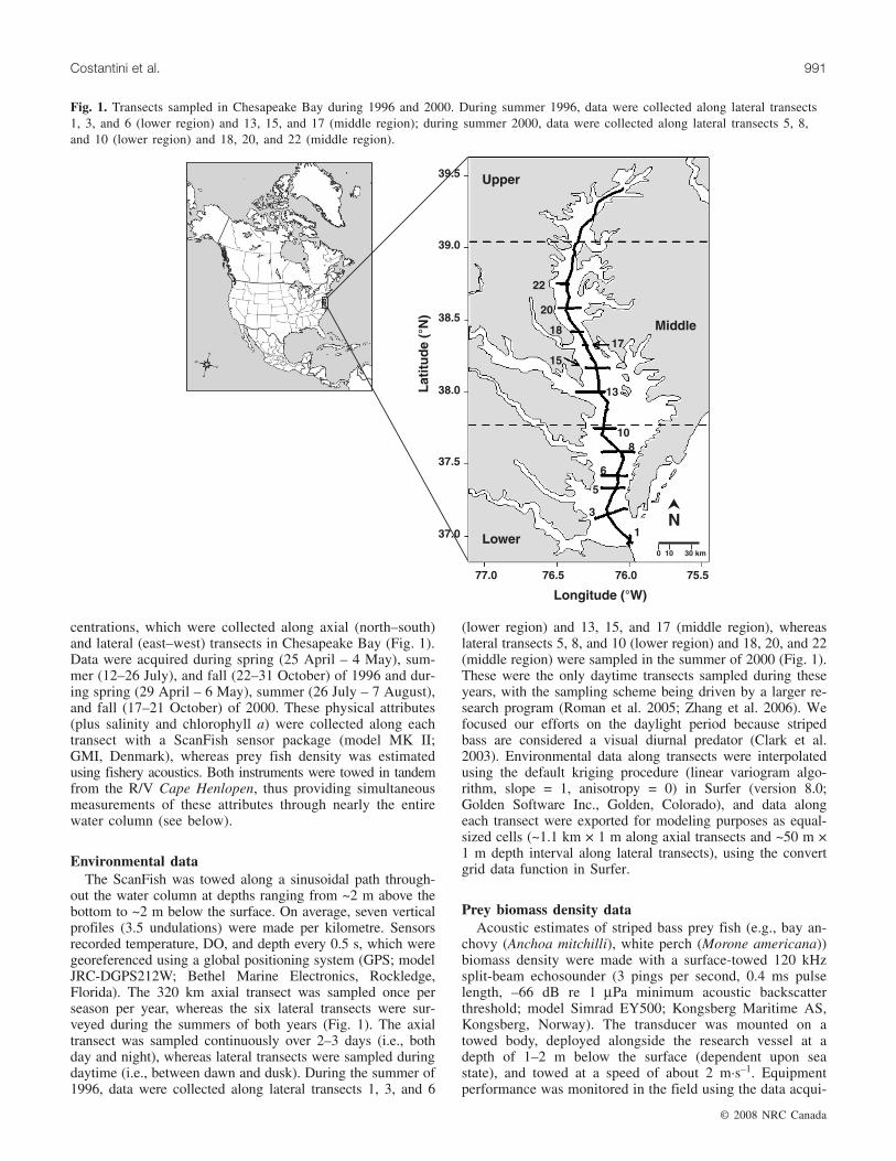
centrations, which were collected along axial (north–south)and lateral (east–west) transects in Chesapeake Bay (Fig. 1).Data were acquired during spring (25 April – 4 May), sum-mer (12–26 July), and fall (22–31 October) of 1996 and dur-ing spring (29 April – 6 May), summer (26 July – 7 August),and fall (17–21 October) of 2000. These physical attributes(plus salinity and chlorophyll a) were collected along eachtransect with a ScanFish sensor package (model MK II;GMI, Denmark), whereas prey fish density was estimatedusing fishery acoustics. Both instruments were towed in tandemfrom the R/V Cape Henlopen, thus providing simultaneousmeasurements of these attributes through nearly the entirewater column (see below).

Environmental dataThe ScanFish was towed along a sinusoidal path through-

out the water column at depths ranging from ~2 m above thebottom to ~2 m below the surface. On average, seven verticalprofiles (3.5 undulations) were made per kilometre. Sensorsrecorded temperature, DO, and depth every 0.5 s, which weregeoreferenced using a global positioning system (GPS; modelJRC-DGPS212W; Bethel Marine Electronics, Rockledge,Florida). The 320 km axial transect was sampled once perseason per year, whereas the six lateral transects were sur-veyed during the summers of both years (Fig. 1). The axialtransect was sampled continuously over 2–3 days (i.e., bothday and night), whereas lateral transects were sampled duringdaytime (i.e., between dawn and dusk). During the summer of1996, data were collected along lateral transects 1, 3, and 6

(lower region) and 13, 15, and 17 (middle region), whereaslateral transects 5, 8, and 10 (lower region) and 18, 20, and 22(middle region) were sampled in the summer of 2000 (Fig. 1).These were the only daytime transects sampled during theseyears, with the sampling scheme being driven by a larger re-search program (Roman et al. 2005; Zhang et al. 2006). Wefocused our efforts on the daylight period because stripedbass are considered a visual diurnal predator (Clark et al.2003). Environmental data along transects were interpolatedusing the default kriging procedure (linear variogram algo-rithm, slope = 1, anisotropy = 0) in Surfer (version 8.0;Golden Software Inc., Golden, Colorado), and data alongeach transect were exported for modeling purposes as equal-sized cells (~1.1 km × 1 m along axial transects and ~50 m ×1 m depth interval along lateral transects), using the convertgrid data function in Surfer.

Prey biomass density dataAcoustic estimates of striped bass prey fish (e.g., bay an-

chovy (Anchoa mitchilli), white perch (Morone americana))biomass density were made with a surface-towed 120 kHzsplit-beam echosounder (3 pings per second, 0.4 ms pulselength, –66 dB re 1 µPa minimum acoustic backscatterthreshold; model Simrad EY500; Kongsberg Maritime AS,Kongsberg, Norway). The transducer was mounted on atowed body, deployed alongside the research vessel at adepth of 1–2 m below the surface (dependent upon seastate), and towed at a speed of about 2 m·s–1. Equipmentperformance was monitored in the field using the data acqui-

© 2008 NRC Canada

Costantini et al. 991

Fig. 1. Transects sampled in Chesapeake Bay during 1996 and 2000. During summer 1996, data were collected along lateral transects1, 3, and 6 (lower region) and 13, 15, and 17 (middle region); during summer 2000, data were collected along lateral transects 5, 8,and 10 (lower region) and 18, 20, and 22 (middle region).

sition software distributed with the Simrad acoustical unit.Raw digitized acoustic signals were time-marked, geocodedusing GPS, and saved to the hard drive for later processing.Calibrations of the Simrad EY500 were performed using astandard 38 mm tungsten carbide reference sphere duringevery cruise (Foote et al. 1987). Identification of acoustictargets was determined by aimed tows of a midwater trawlwith a mouth opening of 18 m2 (for sampling details, seeJung and Houde 2003).

Raw acoustic data were analyzed using Echoview 3.00(SonarData Inc., Hobart, Tasmania, Australia) for standardecho integration and target strength (MacLennan andSimmonds 1992). The blanking distance was set at 1.5 mfrom the transducer and 0.5 m from the bottom, with surfacenoise being identified and omitted from the processing. Datawere subdivided in cells (cell size of 50 m × 1 m depth) andecho-squared integration was performed in each cell. Echo-integration results were initially expressed as relative fishdensity units (Sv) and then scaled by mean backscatter crosssection (σbs) to estimate fish density. Mean backscatter crosssection was estimated using echoes from cells with Nv < 0.1(Rudstam et al. 2003), where Nv = c τ ψ R2nEI, c is the speedof sound (m·s–1), τ is the transmit pulse duration (s), ψ is theequivalent beam angle in steradians, R is the target range

(m), and nEI is the volumetric fish density (number·m–3). In-dividual estimates of σbs were averaged within each cell toprovide σbs. When estimates of σbs were unavailable in acell because of the inability to differentiate individual fishtargets (Nv > 0.1), we calculated σbs using adjacent cells.Number of fish per cubic meter (ρ) in each cell was then cal-culated as ρ = Sv/ σbs.

Fish biomass density per cell (g·m–3) was determined byconverting σbs for each cell to target strength (TS) (σbs =10(TS/10)), and then converting TS to total length (TL) usingTS–TL equations specific to the dominant prey species inthe different regions of Chesapeake Bay (i.e., upper, middle,and lower; Fig. 1). Relationships used for the dominant spe-cies were as follows: bay anchovy TS = 17.9 log(TL) – 66.4(S. Ludsin, unpublished data); white perch TS =26.48 log(TL) – 69.45 (Hartman and Nagy 2005); andalosids (Alosa spp.) TS = 20 log(TL) –76 (Edwards andArmstrong 1984).

Taxa-specific TL was then converted to mass (M) usinglength–mass relationships derived from trawl catches: bay an-chovy M = –13.0956(TL)3.2714; white perch M = –12.3718(TL)3.2457; and alosids M = –11.8614(TL)3.0318 (S. Jung, unpub-lished data; www.chesapeake.org/ties/mwt/SASSAMPL/L-W.htm). Mean mass was multiplied by acoustic-derived fish

© 2008 NRC Canada


Equation Description

GRP prey

pred

= − + + +K

KC R S F U( ( )) Growth rate potential (g·g–1·day–1)

CC B

B=

+max

0.865Consumption (g·g–1·day–1)

Cmax = CA·MCB· fC(T) · fC(DO) Maximum consumption (g·g–1·day–1)

fC(T) = KA·KB Temperature-dependent function (dimensionless)

KL

LA = ⋅

+ ⋅ −CK1 1

1 CK1 1 1( )

L1 = eG1·(T–CQ)

G1 = 1 CTO CQ0.98 1 CK1

CK1 0.02[ /( ] ln

( )− ⋅ ⋅ −⋅

KL

LB = ⋅

+ ⋅ −CK

CK4 2

1 4 2 1( )

L2 = eG2·(CTL–T)

G2 = 1 CTL CTM0.98 1 CK4

CK4 0.02[ /( )] ln

( )− ⋅ ⋅ −⋅

fC(DO) = –0.288 + 0.233(%Sat) – 0.000105(%Sat)2 Dissolved oxygen dependent scale function (dimensionless)

%Sat = 14.4 – 0.332T + 0.00342T 2 Oxygen percent saturation

R = RA·MRB·fR(T)·ACTIVITY Respiration (g·g–1·day–1)

fR(T) = eRQ·T Temperature-dependent function (dimensionless)

ACTIVITY = eRTO Activity multiplier (dimensionless)

S = SDA·(C – F) Specific dynamic action (g·g–1·day–1)

F = FA·C Egestion (g·g–1·day–1)U = UA·(C – F) Excretion (g·g–1·day–1)

Note: Bioenergetics equations were from Hartman and Brandt (1995a); consumption equations were from Brandt et al. (2002);dissolved oxygen function (fC(DO)) was from Brandt et al. (1998); and percent oxygen saturation of the water (%Sat) was fromWetzel (1983). See Table 2 for symbol definitions.

Table 1. Model equations.

© 2008 NRC Canada


density in each cell to calculate prey fish biomass density(g·m–3). Data were then rescaled to conform to the environ-mental data collected by the ScanFish (i.e., to cell size of~1.1 km × 1 m along axial transects and of ~50 m × 1 mdepth along lateral transects), using identical procedures inSurfer, as described above. During the summer of 1996,prey fish biomass density along the axial transect was onlymeasured in the southern part of the middle region and inthe northern part of the lower region because of equipmentproblems, whereas environmental data were collected alongthen entire transect.

Modeling and data analysisGrowth rate potential was quantified along each transect

using previously developed foraging and bioenergeticsgrowth models for striped bass (Tables 1 and 2), assumingthat (i) habitat conditions within a cell were constant for theentire day and were characteristic of the time period (e.g.,season) and (ii) fish predation did not alter the prey biomassdensity (i.e., no density-dependent foraging or feedbackmechanisms existed).

Foraging modelConsumption rate (C; g·g–1·day–1) of striped bass was

modeled using a type II functional response model originallydeveloped for lake trout by Eby et al. (1995) and lateradapted to striped bass by Brandt et al. (2002) (Table 1).Consumption rate in each grid cell along a transect was as-sumed to be a function of striped bass mass, prey fish bio-

mass, water temperature, and DO concentrations by apply-ing a DO-dependent scaling function as in Luo et al. (2001)and Brandt and Mason (2003) (Table 1). Our DO-dependentscaling function, fC(DO), was originally developed byBrandt et al. (1998) for striped bass by fitting experimentallaboratory results to a quadratic model. To summarize, ex-periments were conducted using a 4 × 3 factorial designwith four water temperature treatments (20, 23, 27, and30 °C) and three DO treatments (100% saturation, 4 mg·L–1,and 2 mg·L–1). During each experiment, consumption wasestimated by summing the mass of prey fish consumed.Growth was calculated as the difference between finalweight and initial weight. The quadratic model provided ascalar value between 0 (no food consumption due tohypoxia) and 1.0 (food consumption occurs without any ef-fect of DO), which was used as a multiplier (fC(DO)) to theconsumption model. Striped bass GRP was not affected byDO > 7 mg·L–1, but decreased by about 50% when DO =5 mg·L–1. The minimum DO required for positive GRP var-ied with water temperature, as oxygen saturation concentra-tion is a function of water temperature (Wetzel 1983). Fortemperatures in the range of 12–20 °C, the minimum DO forpositive growth was ~2.5 mg·L–1. As temperature increasedto 20–28 °C, the minimum DO for positive growth increasedfrom 2.5 mg·L–1 to 4.5 mg·L–1. No consumption occurred atDO ≤ 1 mg·L–1 (i.e., fC(DO) = 0.0).

Bioenergetics modelGrowth rate potential (g·g–1·day–1) was calculated in each

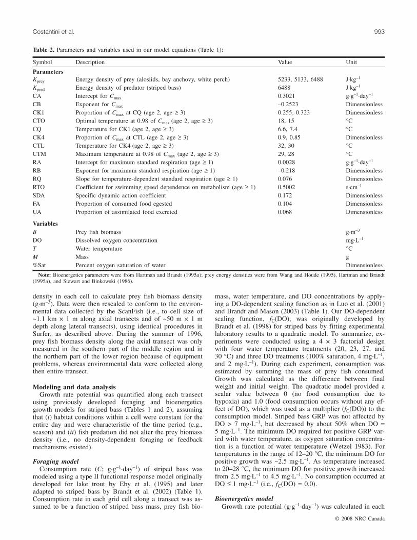
Symbol Description Value Unit

ParametersKprey Energy density of prey (alosiids, bay anchovy, white perch) 5233, 5133, 6488 J·kg–1

Kpred Energy density of predator (striped bass) 6488 J·kg–1

CA Intercept for Cmax 0.3021 g·g–1·day–1

CB Exponent for Cmax –0.2523 DimensionlessCK1 Proportion of Cmax at CQ (age 2, age ≥ 3) 0.255, 0.323 DimensionlessCTO Optimal temperature at 0.98 of Cmax (age 2, age ≥ 3) 18, 15 °CCQ Temperature for CK1 (age 2, age ≥ 3) 6.6, 7.4 °CCK4 Proportion of Cmax at CTL (age 2, age ≥ 3) 0.9, 0.85 DimensionlessCTL Temperature for CK4 (age 2, age ≥ 3) 32, 30 °CCTM Maximum temperature at 0.98 of Cmax (age 2, age ≥ 3) 29, 28 °CRA Intercept for maximum standard respiration (age ≥ 1) 0.0028 g·g–1·day–1

RB Exponent for maximum standard respiration (age ≥ 1) –0.218 DimensionlessRQ Slope for temperature-dependent standard respiration (age ≥ 1) 0.076 DimensionlessRTO Coefficient for swimming speed dependence on metabolism (age ≥ 1) 0.5002 s·cm–1

SDA Specific dynamic action coefficient 0.172 DimensionlessFA Proportion of consumed food egested 0.104 DimensionlessUA Proportion of assimilated food excreted 0.068 Dimensionless

VariablesB Prey fish biomass g·m–3

DO Dissolved oxygen concentration mg·L–1

T Water temperature °CM Mass g%Sat Percent oxygen saturation of water Dimensionless

Note: Bioenergetics parameters were from Hartman and Brandt (1995a); prey energy densities were from Wang and Houde (1995), Hartman and Brandt(1995a), and Stewart and Binkowski (1986).

Table 2. Parameters and variables used in our model equations (Table 1):

cell along transects using the Wisconsin bioenergetics model(Kitchell et al. 1977; Hanson et al. 1997; Table 1) as para-meterized for striped bass (Hartman and Brandt 1995a; Ta-ble 2). Growth was scaled by the relative difference inenergy density between prey and striped bass to account fordifferences in energy density between them (Table 2). Weused prey-specific energy density values from the literature,with the exception of white perch where we used Hartmanand Brandt’s (1995a) striped bass energy density for whiteperch energy density.

We used mean (± standard error, SE) GRP per transect tocompare overall potential growth between 1996 and 2000,using daytime lateral transect data. However, along the axialtransect, we used both day and night data because axial sam-pling started at different hours of the day in the differentyears and so the diurnal sections of the axial transect were

not comparable among years and seasons. As such, compari-sons of axial transect data across season and years should beviewed with some caution.

Effect of hypoxia on habitat qualityWe used a two-step approach to evaluate the effect of

hypoxia on availability of high quality habitat (HQH; i.e., thepercentage of cells that support positive growth along atransect according to Mason et al. 1995). First, we ran thebioenergetics model with and without fC(DO) along eachtransect and compared the GRP values between the two runsusing nonparametric Mann–Whitney U test on untransformeddata, as all GRP data were highly non-normal (P < 0.001;Kolmogorov–Smirnov normality test). Second, for transectsfor which GRP values calculated with and without fC(DO)differed significantly (P < 0.05), we compared HQH obtained

© 2008 NRC Canada


Fig. 2. Seasonal cumulative frequency distributions of (a) water temperature, (b) salinity, (c) dissolved oxygen, and (d) prey biomass den-sity along the axial transect during 1996 (thin lines) and 2000 (thick lines). Because of equipment problems, prey biomass data along theaxial transect in 1996 were only collected in the southern part of the middle region and in the northern part of the lower region.

1996 2000

Variable Spring Summer Fall Spring Summer Fall

Temperature (°C) 10.23±0.03 23.98±0.01 16.65±0.01 13.21±0.01 24.96±0.01 18.08±0.01Salinity 14.33±0.06 15.55±0.08 14.28±0.08 17.12±0.08 17.93±0.07 20.14±0.07Dissolved oxygen (mg·L–1) 8.99±0.05 2.50±0.07 8.40±0.03 10.83±0.06 4.50±0.04 8.67±0.04Prey biomass (g·m–3) 0.03±0.001 0.09±0.02 0.72±0.05 0.42±0.07 6.47±0.67 29.9±2.60No. of cells for environmental variables 4089 3762 5349 5062 4887 5103No. of cells for prey biomass 2223 1205 2477 3028 3231 2349

Note: Environmental and prey biomass data collected along axial transect were subdivided into equal-sized cells; cell sizes were ~ 1.1 km × 1 m and50 m × 1 m for environmental variables and prey biomass, respectively.

Table 3. Mean (±standard error, SE) temperature, dissolved oxygen, salinity, and prey biomass density per cell along the axial transectin Chesapeake Bay during 1996 and 2000.

© 2008 NRC Canada


with fC(DO) with HQH obtained without fC(DO). In so doing,we assumed that the percentage decrease between these twoHQH values represented the magnitude in the reduction of thestriped bass habitat quality due to the oxygen effect.

Results

Environmental conditionsTemperature was cooler for all seasons in 1996 when

compared with 2000 (Fig. 2a; Tables 3 and 4). Overall, aver-age spring (± SE) temperatures were coldest (means 10.23 ±0.03 °C and 13.21 ± 0.01 °C during 1996 and 2000, respec-tively) and summer temperatures were warmest (means23.98 ± 0.01 °C and 24.96 ± 0.01 °C during 1996 and 2000,

respectively), with fall being intermediate (means 16.65 ±0.01 °C and 18.08 ± 0.01 °C during 1996 and 2000, respec-tively). Optimal temperatures for age-2 and age-4 stripedbass growth (i.e., 15–18 °C) were recorded only during fall,whereas temperatures that could potentially reduce growth(i.e., temperatures < 6 °C and temperatures > 28 °C) werenot recorded in either year (Fig. 2a).

Hypoxia and anoxia were more prevalent during the sum-mer of 1996 than during the summer of 2000. Mean (± SE)DO levels were 2.50 ± 0.07 mg·L–1 and 5.50 ± 0.01 mg·L–1

along the axial and lateral transects, respectively, during thesummer of 1996, which were lower than levels along the ax-ial (4.50 ± 0.04 mg·L–1) and lateral (8.66 ± 0.05 mg·L–1)during the summer of 2000, respectively (Tables 3, 4). Dur-

1996 2000

VariableMiddleregion

Lowerregion

Middleregion

Lowerregion

Temperature (°C) 24.62±0.01 23.92±0.01 25.10±0.01 25.83±0.01Salinity 12.15±0.02 20.33±0.04 16.92±0.05 18.92±0.02Dissolved oxygen (mg·L–1) 4.88±0.02 5.50±0.01 8.66±0.05 7.70±0.02Prey biomass (g·m–3) 0.09±0.001 0.01±0.001 16.92±0.02 0.11±0.02No. of cells for environmental variables and prey biomass 11 248 7520 8561 11 406

Note: Environmental and prey biomass data collected along lateral transects were subdivided into equal-sized cells of 50 m longitude × 1 m depth.

Table 4. Mean (± standard error, SE) temperature, dissolved oxygen, salinity, and prey biomass density from pooled lat-eral transects in middle and lower regions of Chesapeake Bay during 1996 and 2000.

Fig. 3. Maps of (a, b) temperature, (c, d) DO, and (e, f) prey biomass along the axial transect in 1996 and 2000. Because of equip-ment problems, prey biomass data along the axial transect in 1996 were only collected in the southern part of the middle region and inthe northern part of the lower region.

ing summer, hypoxia encompassed 62% of the cells sampledduring 1996, but only 48% of the cells sampled during 2000(Fig. 2c). Hypoxia was less of an issue during spring in bothyears, occupying only 7.4% and 11.5% of the sampled watervolume during 1996 and 2000, respectively (Fig. 2c). Duringfall 1996 and 2000, 0% and 5% of the sampled water vol-ume was hypoxic, respectively (Fig. 2c). In spring, fall, andsummer of 2000, anoxic waters occupied <0.3% of the sam-pled volume, whereas in the summer of 1996, anoxic watersoccupied up to 22.5% of the sampled volume (Fig. 2c).

During spring of both years, hypoxia occurred near thebottom (below ~15 m depth) and was limited to the northernpart of the middle region (also see Zhang et al. 2006). Dur-ing summer 1996, hypoxia occupied nearly the entire upperregion (Fig. 3b), all waters below 10 m depth in the middleregion, and deeper waters of the more northerly part of thelower region (Fig. 3b). Similar to 1996, hypoxia was ob-served at depths below 10 m for the entire middle region(Fig. 3e) and in deeper portions of the lower region (Fig. 3e)during 2000; it did occur in the upper region, however. Dur-ing fall of both years, the extent of hypoxia was similar tothat in spring (Zhang et al. 2006).

Prey fish biomass and species compositionDuring 1996 and 2000, the dominant pelagic and bentho-

pelagic fish, which constitute preferred prey of striped bass,were bay anchovy, white perch, blueback herring (Alosaaestivalis), Atlantic herring (Clupea harengus), and otheralosids (Jung and Houde 2003). During all seasons, bay an-chovy was the most abundant prey species in the middle and

lower regions (high salinity areas), whereas white perch wasthe most abundant in the upper region (low salinity areas)(Jung and Houde 2003).

During both years, overall prey fish biomass was lowest inspring and highest in fall, with summer being intermediate(Fig. 2d; Table 3). Overall prey biomass was lower in 1996than in 2000 during all seasons (Fig. 2d; Tables 3 and 4).Summer mean (± SE) fish biomass along the lateral transectsin the middle region was 0.09 ± 0.01 g·m–3 in 1996 com-pared with 16.92 ± 0.02 g·m–3 in 2000, whereas in the lowerregion, fish biomass was 0.01 ± 0.001 g·m–3 in 1996 com-pared with 0.11 ± 0.02 g·m–3 in 2000 (Table 4). Althoughprey abundance and species composition differed betweenyears, nearly all fish prey (>80%) were located in oxygen-ated waters (DO > 4 mg·L–1) during all seasons (Figs. 3b–3f).

Growth rate potential (GRP) and high quality habitat(HQH)

Distributions of GRP, and hence HQH, were similaracross the Bay during both years for age-2 and age-4 stripedbass and closely resembled the pattern of prey–fish biomass.Thus, we have only presented model results for age-2 stripedbass and refer the reader to Appendix A (Table A1) for asummary of age-4 results.

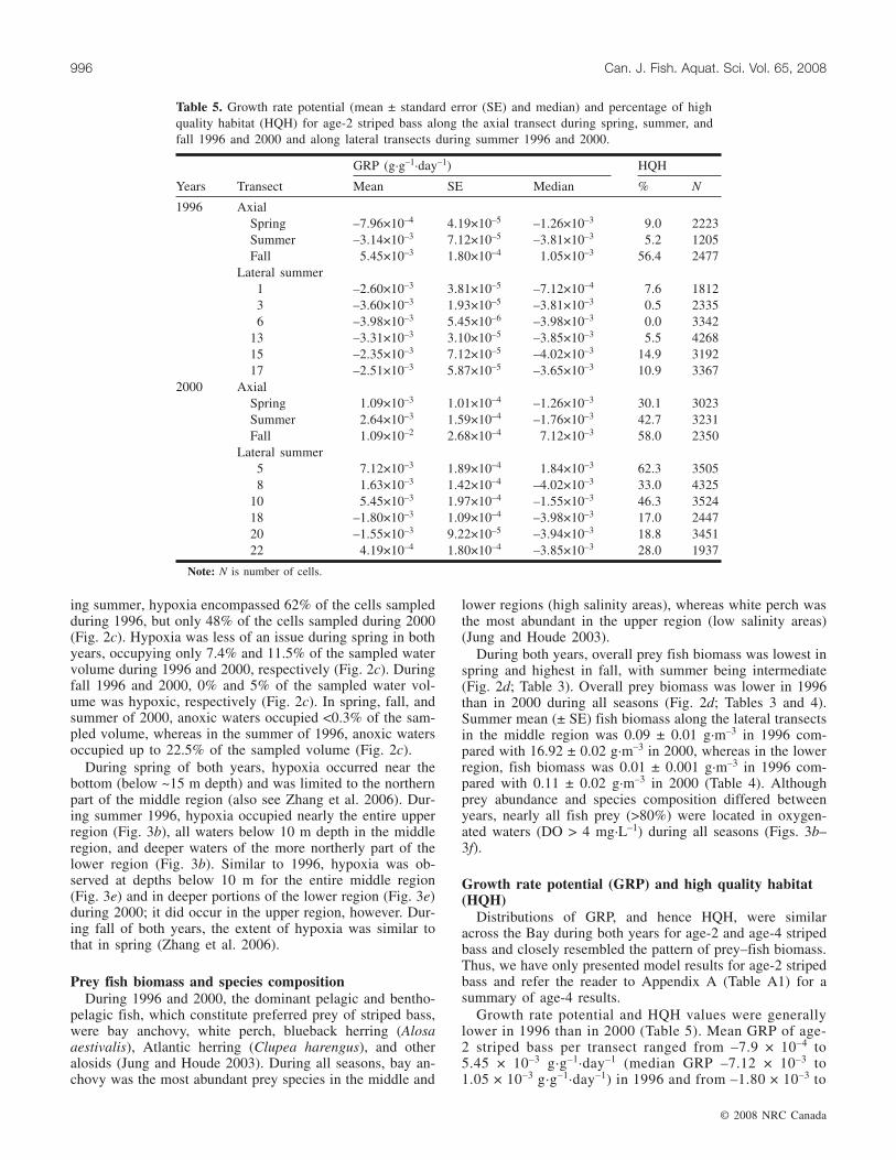
Growth rate potential and HQH values were generallylower in 1996 than in 2000 (Table 5). Mean GRP of age-2 striped bass per transect ranged from –7.9 × 10–4 to5.45 × 10–3 g·g–1·day–1 (median GRP –7.12 × 10–3 to1.05 × 10–3 g·g–1·day–1) in 1996 and from –1.80 × 10–3 to

© 2008 NRC Canada


GRP (g·g–1·day–1) HQH

Years Transect Mean SE Median % N

1996 AxialSpring –7.96×10–4 4.19×10–5 –1.26×10–3 9.0 2223Summer –3.14×10–3 7.12×10–5 –3.81×10–3 5.2 1205Fall 5.45×10–3 1.80×10–4 1.05×10–3 56.4 2477

Lateral summer1 –2.60×10–3 3.81×10–5 –7.12×10–4 7.6 18123 –3.60×10–3 1.93×10–5 –3.81×10–3 0.5 23356 –3.98×10–3 5.45×10–6 –3.98×10–3 0.0 3342

13 –3.31×10–3 3.10×10–5 –3.85×10–3 5.5 426815 –2.35×10–3 7.12×10–5 –4.02×10–3 14.9 319217 –2.51×10–3 5.87×10–5 –3.65×10–3 10.9 3367

2000 AxialSpring 1.09×10–3 1.01×10–4 –1.26×10–3 30.1 3023Summer 2.64×10–3 1.59×10–4 –1.76×10–3 42.7 3231Fall 1.09×10–2 2.68×10–4 7.12×10–3 58.0 2350

Lateral summer5 7.12×10–3 1.89×10–4 1.84×10–3 62.3 35058 1.63×10–3 1.42×10–4 –4.02×10–3 33.0 4325

10 5.45×10–3 1.97×10–4 –1.55×10–3 46.3 352418 –1.80×10–3 1.09×10–4 –3.98×10–3 17.0 244720 –1.55×10–3 9.22×10–5 –3.94×10–3 18.8 345122 4.19×10–4 1.80×10–4 –3.85×10–3 28.0 1937

Note: N is number of cells.

Table 5. Growth rate potential (mean ± standard error (SE) and median) and percentage of highquality habitat (HQH) for age-2 striped bass along the axial transect during spring, summer, andfall 1996 and 2000 and along lateral transects during summer 1996 and 2000.

1.09 × 10–2 g·g–1·day–1 (median GRP –4.02 × 10–3 to7.12 × 10–3 g·g–1·day–1) in 2000 (Table 5). Despite dif-ferences in GRP between years, HQH values were con-sistently lowest during spring, intermediate duringsummer, and highest during fall (Table 5).

During the spring of 1996, mean GRP was negative andonly 9.0% of the sampled volume along the axial transecthad the potential to support positive growth (Table 5). Bycontrast, during spring 2000, mean GRP was positive and30.1% of the total volume had the potential to support posi-tive striped bass growth (Table 5), likely owing to mean preybiomass density being 14-fold higher in 2000 than in 1996(Table 3).

During the summer of 1996, mean GRP values were nega-tive for the axial transect and all lateral transects (Table 5).Along the axial transect, 5.2% of the sampled volume hadthe potential to support positive growth, whereas along lat-eral transects, HQH ranged from 0.0% to 7.6% in the lowerregion and from 5.5% to 14.9% in the middle region. Sum-mer 2000, however, provided a better potential growth envi-ronment for striped bass than summer 1996, owing to thecombination of reduced hypoxia and a more than 70-foldgreater availability of fish prey (Tables 3 and 4; Fig. 3). Av-erage GRP values during 2000 were positive along bothaxial and all lateral transects, except for transects 18 and 20,where some fish prey occurred in hypoxic waters (2.5–3.5 mg·L–1). During the summer of 2000, 42.7% of the axialtransect cells were HQH cells, whereas the percentage ofHQH cells ranged from 33.0% to 62.3% along lateraltransects in the lower region and from 17.0% to 28.0% inthe middle region (Table 5).

Fall of both years were periods of positive growth, owingin large part to high prey densities (Table 3). Mean GRP val-ues were always positive during fall and higher than in bothspring and summer (Table 5). Mean GRP values were lowerin fall 1996 than in fall 2000; however, HQH values weresimilar between years, with 56.4% and 58% of the cells po-tentially supporting positive growth during 1996 and 2000,respectively (Table 5).

Hypoxia effects on GRP and HQHThe effect of fC(DO) on GRP and HQH values varied sea-

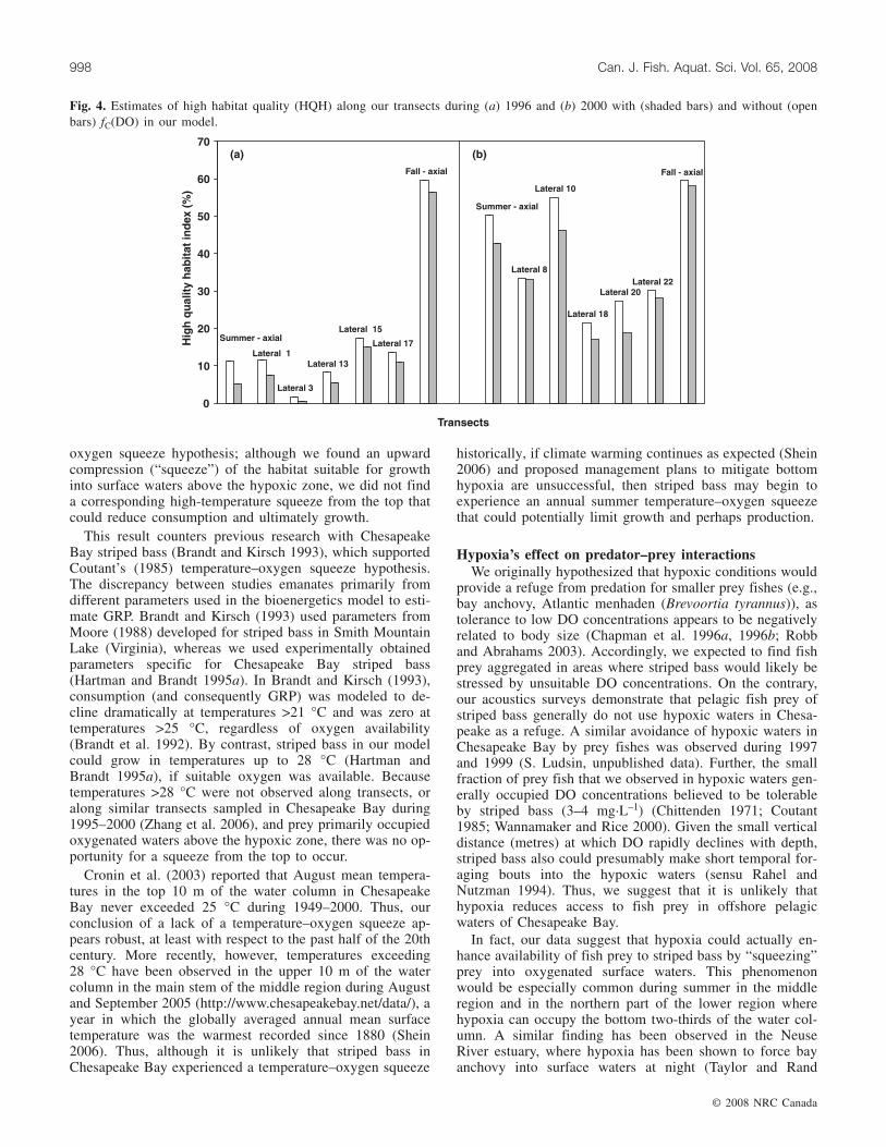
sonally. Our estimates of GRP along lateral transects weresignificantly lower (P < 0.05; Mann–Whitney U test; Ta-ble 6) when fC(DO) was included in our model than withoutit. The only exception was transect 5 (lower region; Fig. 1)during summer 2000 (Table 6); hypoxia was absent alongthis transect. Likewise, along the axial transect, our index ofHQH was always lower using the fC(DO) than without itduring summer and fall of both years (Fig. 4). By contrast,inclusion of the fC(DO) did not cause significant differencesin GRP during spring of both years (Table 6). The percentreductions in HQH owing to the inclusion of fC(DO), how-ever, were generally low, ranging from 1.29% to 6.06% in1996 and from 0.47% to 8.81% in 2000 (Fig. 4).

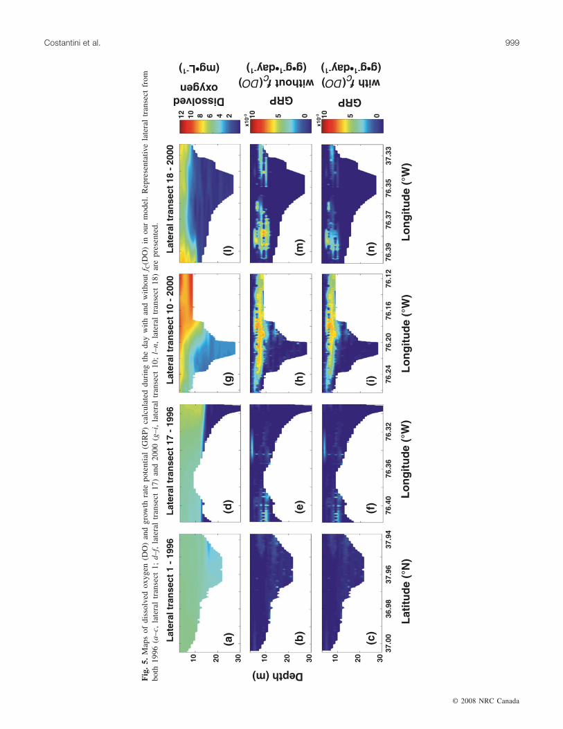
The unexpectedly small reductions in HQH owing to in-clusion of fC(DO) in our model could be attributed to thelack of use of hypoxic waters by fish prey during both years(Figs. 3a–3f). When hypoxia was present along a transect(e.g., transect 17 during summer 1996 (Fig. 5d); transect 10in summer 2000 (Fig. 5g)), positive GRP values occurred

mainly above the hypoxic waters regardless of whether ornot fC(DO) was included in our model (Figs. 5e–5f, 5h–5i).There were instances in which some of the fish prey werefound in hypoxic waters (e.g., transect 18 in summer 2000;Figs. 5l–5n). Although overall GRP values were lower inthese cases, incorporation of fC(DO) did not dramatically re-duce GRP estimates and HQH values (~4.5% reduction;Fig. 4) because these fish were located in waters only justbelow the 4 mg·L–1 isopleth (Fig. 5g). When hypoxia wasnearly absent (e.g., transect 1 during summer 1996;Figs. 5a–5c), positive, but low, GRP values were observedthroughout the water column regardless of whether fC(DO)was included in our model (Figs. 5a–5c).

Discussion

Temperature–oxygen squeeze hypothesisModeled estimates of GRP and our resultant index of

HQH indicate that hypoxia can reduce habitat quality andquantity for striped bass in Chesapeake Bay, primarily dur-ing summer and fall. The observed reduction in HQH due tohypoxia, however, was unexpectedly minor, largely because(i) temperatures in oxygenated surface waters never exceededlevels that could reduce consumption and growth (i.e.,28 °C; Hartman and Brandt 1995a) and (ii) hypoxia did notlimit access to available fish prey for striped bass. Thesefindings only partly support Coutant’s (1985) temperature–

© 2008 NRC Canada


Years Transect p

1996 AxialSpring 0.431Summer <0.0001Fall 0.012

Lateral summer1 0.0013 <0.00016 <0.0001

13 <0.000115 0.01317 <0.0001

2000 AxialSpring 0.052Summer <0.0001Fall <0.0001

Lateral summer5 0.0568 <0.0001

10 <0.000118 <0.000120 <0.000122 <0.0001

Note: Comparisons were made for the axial transect inspring, summer, and fall 1996 and 2000 and for each lateraltransect sampled during summer 1996 and 2000. Where p <0.05, GRP values are lower when fC(DO) was included inthe model than without it.

Table 6. Mann–Whitney U test results from our compari-son of GRP values calculated with and without fC(DO) inour model.

oxygen squeeze hypothesis; although we found an upwardcompression (“squeeze”) of the habitat suitable for growthinto surface waters above the hypoxic zone, we did not finda corresponding high-temperature squeeze from the top thatcould reduce consumption and ultimately growth.

This result counters previous research with ChesapeakeBay striped bass (Brandt and Kirsch 1993), which supportedCoutant’s (1985) temperature–oxygen squeeze hypothesis.The discrepancy between studies emanates primarily fromdifferent parameters used in the bioenergetics model to esti-mate GRP. Brandt and Kirsch (1993) used parameters fromMoore (1988) developed for striped bass in Smith MountainLake (Virginia), whereas we used experimentally obtainedparameters specific for Chesapeake Bay striped bass(Hartman and Brandt 1995a). In Brandt and Kirsch (1993),consumption (and consequently GRP) was modeled to de-cline dramatically at temperatures >21 °C and was zero attemperatures >25 °C, regardless of oxygen availability(Brandt et al. 1992). By contrast, striped bass in our modelcould grow in temperatures up to 28 °C (Hartman andBrandt 1995a), if suitable oxygen was available. Becausetemperatures >28 °C were not observed along transects, oralong similar transects sampled in Chesapeake Bay during1995–2000 (Zhang et al. 2006), and prey primarily occupiedoxygenated waters above the hypoxic zone, there was no op-portunity for a squeeze from the top to occur.

Cronin et al. (2003) reported that August mean tempera-tures in the top 10 m of the water column in ChesapeakeBay never exceeded 25 °C during 1949–2000. Thus, ourconclusion of a lack of a temperature–oxygen squeeze ap-pears robust, at least with respect to the past half of the 20thcentury. More recently, however, temperatures exceeding28 °C have been observed in the upper 10 m of the watercolumn in the main stem of the middle region during Augustand September 2005 (http://www.chesapeakebay.net/data/), ayear in which the globally averaged annual mean surfacetemperature was the warmest recorded since 1880 (Shein2006). Thus, although it is unlikely that striped bass inChesapeake Bay experienced a temperature–oxygen squeeze

historically, if climate warming continues as expected (Shein2006) and proposed management plans to mitigate bottomhypoxia are unsuccessful, then striped bass may begin toexperience an annual summer temperature–oxygen squeezethat could potentially limit growth and perhaps production.

Hypoxia’s effect on predator–prey interactionsWe originally hypothesized that hypoxic conditions would

provide a refuge from predation for smaller prey fishes (e.g.,bay anchovy, Atlantic menhaden (Brevoortia tyrannus)), astolerance to low DO concentrations appears to be negativelyrelated to body size (Chapman et al. 1996a, 1996b; Robband Abrahams 2003). Accordingly, we expected to find fishprey aggregated in areas where striped bass would likely bestressed by unsuitable DO concentrations. On the contrary,our acoustics surveys demonstrate that pelagic fish prey ofstriped bass generally do not use hypoxic waters in Chesa-peake as a refuge. A similar avoidance of hypoxic waters inChesapeake Bay by prey fishes was observed during 1997and 1999 (S. Ludsin, unpublished data). Further, the smallfraction of prey fish that we observed in hypoxic waters gen-erally occupied DO concentrations believed to be tolerableby striped bass (3–4 mg·L–1) (Chittenden 1971; Coutant1985; Wannamaker and Rice 2000). Given the small verticaldistance (metres) at which DO rapidly declines with depth,striped bass also could presumably make short temporal for-aging bouts into the hypoxic waters (sensu Rahel andNutzman 1994). Thus, we suggest that it is unlikely thathypoxia reduces access to fish prey in offshore pelagicwaters of Chesapeake Bay.

In fact, our data suggest that hypoxia could actually en-hance availability of fish prey to striped bass by “squeezing”prey into oxygenated surface waters. This phenomenonwould be especially common during summer in the middleregion and in the northern part of the lower region wherehypoxia can occupy the bottom two-thirds of the water col-umn. A similar finding has been observed in the NeuseRiver estuary, where hypoxia has been shown to force bayanchovy into surface waters at night (Taylor and Rand

© 2008 NRC Canada


Fig. 4. Estimates of high habitat quality (HQH) along our transects during (a) 1996 and (b) 2000 with (shaded bars) and without (openbars) fC(DO) in our model.

© 2008 NRC Canada


Fig

.5.

Map

sof

diss

olve

dox

ygen

(DO

)an

dgr

owth

rate

pote

ntia

l(G

RP

)ca

lcul

ated

duri

ngth

eda

yw

ith

and

wit

hout

f C(D

O)

inou

rm

odel

.R

epre

sent

ativ

ela

tera

ltr

anse

ctfr

ombo

th19

96(a

–c,

late

ral

tran

sect

1;d–

f,la

tera

ltr

anse

ct17

)an

d20

00(g

–i,

late

ral

tran

sect

10;

l–n,

late

ral

tran

sect

18)

are

pres

ente

d.

2003). Likewise, hypoxia has been shown to reduce the diur-nal use of bottom waters by prey fish, resulting in fish being“squeezed” during both day and night into a narrow layer ofwater at or just above the oxycline, where they could bemore vulnerable to striped bass predation (S. Ludsin, unpub-lished data).

This compression of prey into a small area during daylighthours may actually benefit visually feeding striped bass byenhancing predation efficiency and encounter rates with prey.Indeed, hypoxia has been shown to alter predator–prey inter-actions in other ecosystems. For example, Eby and Crowder(2002) demonstrated that hypoxia could increase overlap ofcroaker (Micropogonias undulates), spot (Leiostomus xanthu-rus), and blue crab (Callinectes sapidus) in the Neuse Riverestuary, potentially intensifying both competitive and preda-tory interactions. Eggleston et al. (2005) also indicated thatjuvenile blue crabs may experience increased cannibalism un-der in hypoxia-compressed conditions in the Neuse River es-tuary. Likewise, in Lake Hiidenvesi, Horppila et al. (2003)demonstrated that summer hypoxia and high temperatures insurface waters could squeeze both mysids (Mysis relicta) andsmelt (Osmerus eperlanus) into a narrow layer, resulting inmagnified smelt predation on mysids.

Overall, hypoxia could have opposing short-term effectson striped bass in Chesapeake Bay. In years in which surfacetemperatures exceed 28 °C, hypoxia could negatively affectstriped bass by reducing quality and quantity of habitatthrough a temperature–oxygen squeeze. In cooler years, hy-poxia may benefit striped bass by concentrating prey and in-creasing predator–prey encounter rates in oxygenatedwaters.

Effect of hypoxia on striped bass populationThe recovery of striped bass in Chesapeake Bay occurred

during years characterized by strong summertime hypoxia,consistent with levels observed during our study (Hagy et al.2004). Thus, hypoxia may have played a role in the recoveryby enhancing striped bass foraging efficiency through in-creased prey encounter rates. Given that hypoxia existed inChesapeake Bay prior to the recovery, however, any short-term positive effect of hypoxia on striped bass foraging waslikely secondary relative to reduced mortality experiencedfrom a commercial fishing ban (Richards and Rago 1999).

More recently, however, hypoxia’s elimination of bottomwaters as a refuge for prey fish in much of the middle regionduring summer (S. Ludsin, unpublished data), which wecontend benefited striped bass in the short-term through en-hanced predation efficiency, may actually prove unfavorablefor striped bass production in the long term. At present, alarge striped bass population exists in Chesapeake Bay, pri-marily resulting from management actions that placed re-strictions on harvest (Richards and Rago 1999). In turn,recent field and modeling studies suggest that striped basspredatory demand may be exceeding the capacity of the Bayto support the current striped bass population and that insuf-ficient prey resources are likely responsible for recent (post-1995) reductions in striped bass growth and condition, aswell as the increased prevalence of pathologies associatedwith malnutrition (Hartman and Brandt 1995b; Overton etal. 2003; Uphoff 2003). Indeed, Atlantic menhaden, whichwas historically the dominant prey of striped bass in Chesa-

peake Bay, is at very low levels, likely due to both overfish-ing and striped bass predation (Uphoff 2003). Likewise, bayanchovy recruitment is at record low levels (www.dnr.state.md.us/fisheries/juvindex/index.html#Indices), and consump-tion of bay anchovy by striped bass in recent years has in-creased relative to historical levels (Overton 2002; Griffinand Margraf 2003).

In summary, our results suggest that a temperature–oxygen squeeze historically has not limited growth of stripedbass, but it may become important if climate warming in theregion continues along its current trajectory (Shein 2006).Moreover, hypoxia may have indirectly benefited stripedbass by increasing their foraging efficiency and, in this way,may have contributed to their recovery during the mid-1990s. However, although hypoxia may have benefitedstriped bass in the short term by providing access to moreprey, the loss of bottom refugia for fish prey may ultimatelylead to long-term negative consequences for the populationby allowing the forage base to be overconsumed. Althoughmore research is required to test the relevance of these hy-potheses, our data clearly suggest that Chesapeake Bayagencies need to consider the effect of hypoxia when man-aging both striped bass and their prey.

Acknowledgments

The field program for this research was made possible bythe NSF – Land Margin Ecosystem Research Program pro-ject “Trophic Interactions in Estuarine Systems” (TIES;DEB-9412133). The Sloan Foundation Census of MarineLife (CoML) program (2001-3-8) supported the synthesis offield data. We also acknowledge the crew of the R/V CapeHenlopen and assistance in data collection and analysis byH. Adolf, C. Derry, L. Florence, E. Graham, C. Hand, D.Hondorp, J. Hawkey, C. McGilliard, S. Pothoven, C. Rae, J.Reichert, A. Sanford, A. Spear, and T. Wazniak. This isNOAA–GLERL contribution No. 1445.

References

Aku, P.M.K., and Tonn, W.M. 1999. Effects of hypolimnetic oxy-genation on the food resources and feeding ecology of cisco inAmisk Lake, Alberta. Trans. Am. Fish. Soc. 128: 17–30.

Boesch, D.F., Brinsfield, R.B., and Magnien, R.E. 2001. Chesa-peake Bay eutrophication: scientific understanding, ecosystemrestoration, and challenges for agriculture. J. Environ. Qual. 30:303–320.

Boynton, W.R., Garber, J.H., Summers, R., and Kemp, W.M. 1995.Inputs, transformations, and transport of nitrogen and phospho-rus in Chesapeake Bay and selected tributaries. Estuaries, 18:285–314.

Brandt, S.B., and Kirsch, J. 1993. Spatially explicit models ofstriped bass growth potential in the Chesapeake Bay. Trans. Am.Fish. Soc. 122: 845–869.

Brandt, S.B., and Mason, D.M. 2003. Effect of nutrient loading onAtlantic menhaden Brevoortia tyrannus growth rate potential inthe Patuxent River. Estuaries, 26: 298–309.

Brandt, S.B., Mason, D.M., and Patrick, E.V. 1992. Spatially-explicitmodels of fish growth rate. Fisheries, 17: 23–35.

Brandt, S.B., Demers, E., Tyler, A.J., and Gerken, M.A. 1998. Fishbioenergetics modeling. Chesapeake Bay Ecosystem ModelingProgram (1993–1998), Report to the Chesapeake Bay Program. US

© 2008 NRC Canada


Environmental Protection Agency, Chesapeake Bay Program Of-fice, 410 Severn Avenue, Suite 109, Annapolis, MD 21403, USA.

Brandt, S.B., Mason, D.M., McCormick, M.J., Lofgren, B., Hunter,T.S., and Tyler, J.A. 2002. Climate change: implications for fishgrowth performance in the Great Lakes. Am. Fish. Soc. Symp.32: 61–76.

Breitburg, D.L., Pihl, L., and Kolesar, S.E. 2001. Effects of lowdissolved oxygen on the behavior ecology and harvest of fishes:a comparison of the Chesapeake Bay and Baltic–Kattegat sys-tems. In Coastal hypoxia: consequences for living resources andecosystems. Edited by N.N. Rabalais and R.E. Turner. AmericanGeophysical Union, Washington, D.C. pp. 241–268.

Caddy, J.F. 1993. Toward a comparative evaluation of human im-pacts on fishery ecosystems of enclosed and semi-enclosed seas.Rev. Fish. Sci. 1: 57–95.

Carpenter, S.R., Caraco, N.F., Correll, D.L., Howarth, R.W., Sharpley,A.N., and Smith, V.H. 1998. Nonpoint pollution of surface waterswith phosphorus and nitrogen. Ecol. Appl. 8: 559–568.

Chapman, L.J., Chapmann, C.A., and Chandler, M. 1996a. Wet-lands ecotones as refugia for endangered fishes. Biol. Conserv.78: 263–270.

Chapman, L.J., Chapmann, C.A., Ogutu-Ohwayo, R., Chandler,M., Kaufman L.S., and Keiter, A.E. 1996b. Refugia for endan-gered fishes from an introduced predator in Lake Nabugabo,Uganda. Conserv. Biol. 10: 554–561.

Chittenden, M.E., Jr. 1971. Status of the striped bass Morone saxatilisin the Delaware River. Chesapeake Sci. 12: 131 136.

Clark, K.L., Ruiz, G.M., and Hines, A.H. 2003. Diel variation inpredator abundance predation risk and prey distribution inshallow-water estuarine habitats. J. Exp. Mar. Biol. Ecol. 287:37–55.

Cloern, J.E. 2001. Our evolving conceptual model of the coastaleutrophication problem. Mar. Ecol. Prog. Ser. 210: 223–253.

Cooper, S.R., and Brush, G.S. 1991. Long-term history of Chesa-peake Bay anoxia. Science (Washington, D.C.), 254: 992–996.

Coutant, C.C. 1985. Striped bass temperature and dissolved oxy-gen: a speculative hypothesis for environmental risk. Trans. Am.Fish. Soc. 114: 31–61

Cronin, T.M., Dwyer, G.S., Kamiya, T., Schwede, S., and Willard,D.A. 2003. Medieval Warm Period, Little Ice Age and 20th cen-tury temperature variability from Chesapeake Bay. Global PlanetChange, 36: 17–29.

Diaz, R.J., and Rosenberg, R. 1995. Marine benthic hypoxia: a reviewof its ecological effects and the behavioural responses of benthicmacrofauna. Oceanogr. Mar. Biol. Annu. Rev. 33: 245–303.

Eby, L.A., and Crowder, L.B. 2002. Hypoxia-based habitat com-pression in the Neuse River Estuary: context-dependent shifts inbehavioral avoidance thresholds. Can. J. Fish. Aquat. Sci. 59:952–965.

Eby, L.A., Rudstam, L.G., and Kitchell, J.F. 1995. Predator responsesto prey population dynamics: an empirical analysis based on laketrout growth rates. Can. J. Fish. Aquat. Sci. 52: 1564–1571.

Edwards, J.I., and Armstrong, F. 1984. Target strength experimentson caged fish. Scott. Fish. Bull. 48: 12–20.

Eggleston, D.B., Bell, G.W., and Amavisca, A.D. 2005. Interactiveeffects of episodic hypoxia and cannibalism on juvenile bluecrab mortality. J. Exp. Mar. Biol. Ecol. 325: 18–26.

Foote, K.G., Knudsen, H.P., Vestnes, G., MacLennan, D.N., andSimmonds, E.J. 1987. Calibration of acoustic instruments forfish density estimation: a practical guide. ICES Coop. Res. 144:1–69.

Griffin, J.C., and Margraf, F.J. 2003. The diet of Chesapeake Baystriped bass in the late 1950s. Fish. Manag. Ecol. 10: 323–328.

Hagy, J.D., Boynton, W.R., Keefe, C.W., and Wood, K.V. 2004.Hypoxia in Chesapeake Bay, 1950–2001: long-term change in re-lation to nutrient loading and river flow. Estuaries, 27: 634–658.

Hanson, P.C., Johnson, T.B., Schindler, D.E., and Kitchell, J.F. 1997.Fish bioenergetics 3.0 for Windows. University of Wisconsin–Madison, Madison, Wis.

Hartman, K.J., and Brandt, S.B. 1995a. Comparative energetics andthe development of bioenergetics models for sympatric estuarinepiscivores. Can. J. Fish. Aquat. Sci. 52: 1647–1666.

Hartman, K.J., and Brandt, S.B. 1995b. Predatory demand and im-pact of striped bass, bluefish, and weakfish in the ChesapeakeBay: applications of bioenergetics models. Can. J. Fish. Aquat.Sci. 52: 1667–1687.

Hartman, K.J., and Margraf, F.J. 2003. US Atlantic coast stripedbass: issues with a recovered population. Fish. Manag. Ecol. 10:309–312.

Hartman, K.J., and Nagy, B.W. 2005. A target strength and lengthrelationship for striped bass and white perch. Trans. Am. Fish.Soc. 134: 375–380.

Horppila, J., Liljendahl-Nurminen, A., Malinen, T., Salonen, M.,Tuomaala, A., Uusitalo, L., and Vinni, M. 2003. Mysis relicta in aeutrophic lake: consequences of obligatory habitat shifts. Limnol.Oceanogr. 48: 1214–1222.

Jung, S., and Houde, E.D. 2003. Spatial and temporal variability ofpelagic fish community structure and distribution in ChesapeakeBay, USA. Est. Coast. Shelf. Sci. 58: 335–351.

Kemp, W.M., Boynton, W.R., Adolf, J.E., Boesch, D.F., Boicourt,W.C., Brush, G., Cornwell, J.C., Fisher, T.R., Glibert, P.M., Hagy,J.D., Harding, L.W., Houde, E.D., Kimmel, D.G., Miller, W.D.,Newell, R.I.E., Roman, M.R., Smith, E.M., and Stevenson, J.C.2005. Eutrophication of Chesapeake Bay: historical trends andecological interactions Mar. Ecol. Prog. Ser. 303: 1–29.

Kitchell, J.F., Stewart, D.J., and Weininger, D. 1977. Applicationsof a bioenergetics model to yellow perch, Perca flavescens, andwalleye, Stizostedion vitreum vitreum. J. Fish. Res. Board. Can.34: 1922–1935.

Luo, J., Hartman, K.J., Brandt, S.B., Cerco, C.F., and Rippetoe,T.H. 2001. A spatially-explicit approach for estimating carryingcapacity: an application for the Atlantic menhaden Brevoortiatyrannus in Chesapeake Bay. Estuaries, 24: 545–556.

MacLennan, D.N., and Simmonds, E.J. 1992. Fisheries acoustics.1st ed. Chapman and Hall, London, UK.

Mansueti, R.J. 1961. Age, growth, and movements of the stripedbass, Rocco saxatilis, taken in select fishing gear in Maryland.Chesapeake Sci. 2: 9–36.

Mason, D.M., Goyke, A., and Brandt, S.B. 1995. A spatially explicitbioenergetics measure of habitat quality for adult salmonines —comparison between Lakes Michigan and Ontario. Can. J. Fish.Aquat. Sci. 52: 1572–1583.

Moore, C.M. 1988. Food habits, population dynamics, and bio-energetics of four predator fish species in Smith Mountain Lake,Virginia. Ph. D. thesis, Virginia Polythecnical Institute and StateUniversity, Blacksburg, Virginia.

Officer, C.B., Biggs, R.B., Taft, J.L., Cronin, L.E., Tyler, M.A., andBoynton, W.R. 1984. Chesapeake Bay anoxia: origin, develop-ment, and significance. Science (Washington, D.C.), 223: 22–26.

Overton, A.S. 2002. Striped bass predator–prey interactions in Ches-apeake Bay and along the Atlantic Coast. Ph.D. dissertation, Uni-versity of Maryland–Eastern Shore, Princess Anne, Maryland.

Overton, A.S., Margraf, F.J., Weedon, C.A., Pieper, L.H., and May,E.B. 2003. The prevalence of mycobacterial infections in stripedbass in Chesapeake Bay. Fish. Manag. Ecol. 10: 301–308.

Rabalais, N.N., Turner, R.E., Dortch, Q., Justic, D., Bierman, V.J.,Jr., and Wiseman, W.J., Jr. 2002. Nutrient-enhanced productivity

© 2008 NRC Canada


in the northern Gulf of Mexico: past, present and future. Hydro-biologia, 475: 39–63.

Rahel, F.J., and Nutzman, J.W. 1994. Foraging in a lethal environ-ment: fish predation in hypoxic waters of a stratified lake. Ecol-ogy, 75: 1246–1253.

Richards, R.A., and Rago, P.J. 1999. A case history of effectivefishery management: Chesapeake Bay striped bass. N. Am. J.Fish. Manag. 19: 356–375.

Robb, T., and Abrahams, M.V. 2003. Variation in tolerance tohypoxia in a predator and prey species: an ecological advantageof being small? J. Fish Biol. 62: 1067–1081.

Roman, M.R., Gauzens, A.L., Rhinehart, W.K., and White, J.R.1993. Effects of low oxygen waters on Chesapeake Bay zoo-plankton. Limnol. Oceanogr. 38: 1603–1614.

Roman, M.R., Zhang, X., McGilliard, C., and Boicourt, W.C. 2005.Seasonal and annual variability in the spatial patterns of planktonbiomass in Chesapeake Bay. Limnol. Oceanogr. 50: 480–492.

Rudstam, L.G., Parker, S.L., Einhouse, D.W., Witzel, L.D., Warner,D.M., Stritzel, J.L., Parrish, D.L., and Sullivan, P.J. 2003. Appli-cation of in situ target-strength estimations in lakes: examplesfrom rainbow-smelt surveys in Lakes Erie and Champlain. ICESJ. Mar. Sci. 60: 500–507.

Secor, D.H., and Piccoli, P.M. 2007. Oceanic migration rates of up-per Chesapeake Bay striped bass (Morone saxatilis), determinedby otolith microchemical analysis. Fish. Bull. 105: 62–73.

Shein, K.A. 2006. State of the climate in 2005. Bull. Am. Meteorol.Soc. 87: 1–102.

Stewart, D.J., and Binkowski, F.P. 1986. Dynamics of consumptionand food conversion by Lake Michigan alewives: an energetics-modeling synthesis. Trans. Am. Fish. Soc. 115: 643–661.

Taylor, J.C., and Rand, P.S. 2003. Spatial overlap and distributionof anchovies (Anchoa spp.) and copepods in a shallow stratifiedestuary. Aquat. Living Resour. 16: 191–196.

Uphoff, J.H. 2003. Predator–prey analysis of striped bass and At-lantic menhaden in upper Chesapeake Bay. Fish. Manag. Ecol.10: 313–322.

Wang, S.B., and Houde, E.D. 1995. Distribution, relative abun-dance, biomass and production of bay anchovy Anchoa mitchilliin the Chesapeake Bay. Mar. Ecol. Prog. Ser. 121: 27–38.

Wannamaker, C.M., and Rice, J.A. 2000. Effects of hypoxia onmovements and behavior of selected estuarine organisms fromthe south-eastern United States. J. Exp. Mar. Biol. Ecol. 249:145–163.

Wetzel, R.G. 1983. Limnology. 2nd ed. Saunders College Pub-lishing, Toronto, Ontario, Canada.

Zhang, X., Roman, M., Kimmel, D., McGilliard, C., and Boicourt,W.C. 2006. Spatial variability in plankton biomass and hydro-graphic variables along an axial transect in Chesapeake Bay. J.Geophys. Res. Oceans, 111: C05S11, doi:10.1029/2005JC003085.

Appendix A

© 2008 NRC Canada


GRP (g·g–1·day–1) HQH

Years Transect Mean SE Median % N

1996 AxialSpring –5.03×10–4 3.06×10–5 –8.38×10–4 9.0 2223Summer –2.14×10–3 4.61×10–5 –2.56×10–3 5.2 1205Fall 3.44×10–3 1.17×10–4 6.29×10–4 56.4 2477

Lateral summer1 –1.80×10–3 2.43×10–5 –2.05×10–3 7.6 18123 –2.43×10–3 1.22×10–5 –2.60×10–3 0.5 23356 –2.68×10–3 3.65×10–6 –2.68×10–3 0.0 3342

13 –2.26×10–3 1.97×10–5 –2.60×10–3 5.5 426815 –1.68×10–3 4.61×10–5 –2.72×10–3 14.9 319217 –1.76×10–3 3.73×10–5 –2.43×10–3 10.9 3367

2000 AxialSpring 7.96×10–4 6.70×10–5 –8.38×10–4 30.1 3023Summer 1.51×10–3 1.01×10–4 –1.30×10–3 42.7 3231Fall 6.70×10–3 1.72×10–4 4.19×10–3 58.0 2350

Lateral summer5 4.19×10–3 1.22×10–4 1.01×10–3 62.3 35058 8.80×10–4 9.22×10–5 –2.72×10–3 33.0 4325

10 3.27×10–3 1.26×10–4 –1.13×10–3 46.3 352418 –1.34×10–2 7.12×10–5 –2.68×10–3 17.0 244720 –1.01×10–3 6.29×10–5 –2.68×10–3 18.8 345122 1.05×10–4 1.13×10–4 –2.60×10–3 28.0 1937

Note: N is number of cells.

Table A1. Growth rate potential (GRP; mean ± standard error (SE), median) and percentage ofhigh quality habitat (HQH) for age-4 striped bass along the axial transect during spring, summer,and fall 1996 and 2000, and along lateral transects during summer 1996 and 2000.

effect of hypoxia on habitat quality of striped bass ... · effect of hypoxia on habitat quality of...

Documents