effect of particle filling and size on the behaviour of
TRANSCRIPT

EFFECT OF PARTICLE FILLING AND SIZE ON
THE BEHAVIOUR OF THE BALL LOAD AND
POWER IN A DRY MILL
Kiangi Kimera Kiangi
A thesis submitted to the Faculty of Engineering and the Built
Environment, University of the Witwatersrand, Johannesburg, in
fulfilment of the requirements for the degree of Doctor of
Philosophy.
Johannesburg, 2011

i
DECLARATION
I declare that this thesis is my own, unaided work. It is being submitted for
the Degree of Doctor of Philosophy in the University of the Witwatersrand,
Johannesburg. It has not been submitted before for any degree or
examination in any other University.

ii
If I have seen further, it is by standing upon the
shoulders of giants.
- Sir Isaac Newton
If one is to stand on the shoulders of giants, one must
first climb up their backs; and the greater the body of
knowledge, the harder this climb becomes.
- Benjamin Jones (Professor at the Kellogg School of Management, Northwestern University)
iii
ABSTRACT
This study on the effects of particle filling and size on the ball load
behaviour and power in a dry mill was initiated at the University of the
Witwatersrand in 2003. The aim of the study was to make available a
better understanding of the underlying causes in the different power draws
that occur in mills when ore particles are being added to the ball load. This
mimics the process of filling an industrial grinding mill after a grind out has
been performed. Typically after a grind out, the mill operator would refill
the mill with ore up to the point where maximum mill power draw is
registered. At maximum power draw it is assumed that the void spaces
within the ball load are filled with ore particles and that the charge is well
mixed.
In order to conduct the study an inductive proximity probe was used to
measure the dynamics of the load behaviour. This novel technique in
measuring load behaviour was chosen due to the fact that the probe could
sense the presence of steel balls independent of the presence of particles
in the mill. The probe’s response to a load comprised of steel balls only at
the fillings of 15-45% and mill speeds of 60 – 105% indicate that the
various changes in load behaviour such as cataracting, centrifuging, ball
packing and toe and shoulder responses were easily distinguished in
probes responses. Further tests were conducted in a mill with a 20% ball
filling with increasing coarse or fine silica sand particle filling from 0 –
150% at the mill speeds of 63-98% of the critical mill speed. These tests

iv
clearly reveal radial segregation of coarse silica sand, increased ball
cataracting and centrifuging of just silica sand or a combination of balls
and silica sand. The impacts of these phenomena have been discussed
with reference to industrial mills.
The physical parameters defining the load provided by the inductive probe
made it interesting to make use of Morrell’s C model to simulate the power
drawn by the mill. Modifications to Morrell’s model were made thus leading
to a modification in the toe and shoulder model and proposals for a
segregated charge model, a centrifuged charge model and a particle pool
model. Furthermore a modelling study based on the torque-arm modelling
approach was conducted. Here Moys power model was used to study the
effect increasing coarse and fine particle filling has on the power drawn by
a mill. A liner model was proposed to define N* as a function of particle
filling. In both modelling cases the models were used to account for the
various conditions arising within the load as particle filling and mill speed
increases.

v
DEDICATION
I dedicate this thesis to my wonderful parents, Dr. Peter M R Kiangi and
Mrs. Helen W Kiangi, who have shown devotion, passion and unending
support for my personal development and growth from childhood right up
to now. God bless you both to live a long and happy life.

vi
ACKNOWLEDGEMENTS
It is my pleasure to thank the people who made this thesis possible.
It is difficult to overstate my gratitude towards my PhD supervisor
Professor M H Moys who took me under his wing and showed me how to
use my previously gained undergraduate engineering knowledge in
conducting mineral processing research. His enthusiasm, guidance,
inspiration and occasional encouragement to push forward with my thesis
will be forever cherished. Prof. Moys has been a true friend, advisor and
mentor to me. I shall be forever indebted to him. Thank you very much.
I am also indebted to my fellow colleagues in Prof. Moys research group
who provided a stimulating, fun and challenging environment to learn and
grow. I am especially grateful to Dr M. Bwalya, Dr. H Dong, Mr. G Finnie,
Mr C Couvas, Dr. J Kalala, Mr. G Monama, Mr L Niyoshaka and Mr A
Makokha.
I am also grateful to the workshop staff who tirelessly worked on my
requests to fabricate the necessary experimental equipment that I
required.
I wish to thank my close friend and countryman, Dr. T Mwakabaga, who
lent me his ears during my times of doubt. He has also been a good guide
to my pursuit towards improving my computer programming skills.

vii
Last but by no means least; I would like to thank God for blessing me
throughout my life. He has blessed me with this journey through Wits and
afforded me the opportunity to work under a great African scientist Prof.
Moys.
============ Ahsante Sana Na Mungu Awabariki1 ==============
.
1 Swahili for Thank you very much and may God bless you all

viii
TABLE OF CONTENTS
DECLARATION ......................................................................................... IABSTRACT ............................................................................................. IIIDEDICATION ........................................................................................... VACKNOWLEDGEMENTS ....................................................................... VITABLE OF CONTENTS ........................................................................ VIIILIST OF FIGURES ................................................................................. XILIST OF TABLES ................................................................................. XIV
CHAPTER 1INTRODUCTION ................................................................... 11.0 INTRODUCTION ................................................................................. 21.2 OBJECTIVE OF THE THESIS ............................................................ 31.3 THESIS OUTLINE .............................................................................. 3
CHAPTER 2 LITERATURE REVIEW ........................................................ 72.0 INTRODUCTION ................................................................................ 82.1 LOAD BEHAVIOUR MEASUREMENT TECHNIQUES ...................... 14
2.1.1 ACOUSTIC EMISSION MEASUREMENT TECHNIQUE .................................................. 152.1.2 CONDUCTIVITY MEASUREMENT TECHNIQUE ........................................................... 172.1.3 VIBRATIONS MEASUREMENT TECHNIQUE ............................................................... 192.1.4 MOVEMENT, PRESSURE OR FORCE MEASUREMENT TECHNIQUE .............................. 222.1.5 X-RAY MEASUREMENT TECHNIQUE ....................................................................... 26
2.2 MODELS FOR MILL POWER ........................................................... 282.2.1 EMPIRICAL MILL POWER MODELS ......................................................................... 29
2.2.1.1 Rose and Sullivan’s Power Model .............................................................. 312.2.1.2 Bond’s Power Model.................................................................................. 332.2.1.3 Fuerstenau, Kapur and Velamakanni’s Power Model ................................. 342.2.1.4 Moys Power Model .................................................................................... 372.2.1.5 Morrell’s Power Model ............................................................................... 41
2.2.2 MECHANISTIC MILL POWER MODELS..................................................................... 452.2.2.1 The Discrete Element Method (DEM) ........................................................ 46
2.3 CONCLUSION .................................................................................. 50
CHAPTER 3 MEASUREMENT TECHNIQUE.......................................... 523.0 INTRODUCTION ............................................................................... 533.1 THE INDUCTIVE PROXIMITY PROBE ............................................. 543.2 EXPERIMENTAL EQUIPMENT AND METHOD ................................ 56

ix
3.3 INDUCTIVE PROXIMITY PROBE SIGNAL ANALYSIS ..................... 563.3.1 DESCRIPTION OF THE INDUCTIVE PROXIMITY PROBE’S SIGNAL ................................. 59
3.4 EXPERIMENTAL RESULTS AND ANALYSIS ................................... 623.4.1 INDUCTIVE PROXIMITY PROBE’S SIGNAL AS A FUNCTION OF MILL SPEED .................. 623.4.2 INDUCTIVE PROXIMITY PROBE’S SIGNAL AS A FUNCTION OF MILL FILLING ................. 653.4.3 LOAD ORIENTATION AS A FUNCTION OF MILL SPEED AND MILL FILLING ..................... 673.4.4 COMPARISON OF THE INDUCTIVE PROBE WITH THE FORCE PROBE ........................... 68
3.5 CONCLUSION .................................................................................. 70
CHAPTER 4 EXPERIMENTAL STUDY .................................................. 714.0 INTRODUCTION ............................................................................... 724.1 EXPERIMETAL EQUIPMENT AND METHOD ................................... 734.2 RESULTS AND DISCUSSIONS ........................................................ 76
4.2.1 EFFECT OF PARTICLE FILLING AND PARTICLE SIZE ON THE NET POWER ...................... 764.2.2 EFFECT OF PARTICLE FILLING AND PARTICLE SIZE ON THE BALL LOAD BEHAVIOUR ....... 78
4.3 RADIAL SEGREGATION WITHIN THE LOAD .................................. 854.4 EFFECT OF REDUCING THE CHANGE IN PARTICLE SIZE
DISTRIBUTION................................................................................. 894.5 CONCLUSION .................................................................................. 90
CHAPTER 5 MODELLING STUDY 1 ...................................................... 935.0 INTRODUCTION ............................................................................... 945.1 MORRELL’S MODEL ........................................................................ 955.2 ANALYSIS AND DISCUSSIONS ....................................................... 97
5.2.1 MODELLING OF THE COARSE PARTICLE EFFECTS ..................................... 985.2.2 MODELLING THE EFFECTS OF RADIAL SEGREGATION ............................. 1065.2.3 MODELLING OF THE FINE PARTICLE EFFECTS .......................................... 113
5.3 CONCLUSION ................................................................................ 118
CHAPTER 6 MODELLING STUDY 2 .................................................... 1206.0 INTRODUCTION ............................................................................. 1216.1 MOYS POWER MODEL FRAMEWORK ......................................... 1216.2 ANALYSIS AND DISCUSSIONS ..................................................... 124
6.2.1 MODELLING OF COARSE PARTICLE EFFECTS ON POWER ....................... 1256.2.2 MODELLING OF THE FINE PARTICLE EFFECTS ON POWER ...................... 130
6.3 CONCLUSION ................................................................................ 134

x
CHAPTER 7 CONCLUSION AND RECOMMENDATION ..................... 1377.0 CONCLUSION ................................................................................ 138
REFERENCES ..................................................................................... 147
APPENDIX 1 ......................................................................................... 155A1.1 EXPERIMENTAL DATA FOR THE COARSE PARTICLE
EXPERIMENTS .............................................................................. 156A1.2 EXPERIMENTAL DATA FOR THE FINE PARTICLE EXPERIMENTS
....................................................................................................... 158
APPENDIX 2 ......................................................................................... 160A2.1 MIXED CHARGE MODELLING..................................................... 161A2.2 CENTRIFUGED CHARGE MODELLING ...................................... 167A2.3 SEGREGATED CHARGE MODELLING ....................................... 179A3.4 POOL POWER MODELLING USING SIMPSON’S METHOD ....... 187A2.5 MATLAB PROGRAM: POOL’S TORQUE AND POWER ............... 195
APPENDIX 3 ......................................................................................... 207A3.1 REGRESSION ON BALLS ONLY DATA ....................................... 208A3.2 REGRESSION ON POWER DATA FROM COARSE PARTICLE
EXPERIMENTS .............................................................................. 210A3.3 REGRESSION ON POWER DATA FROM FINE PARTICLE
EXPERIMENTS .............................................................................. 218

xi
LIST OF FIGURES
Chapter 2Figure 2.1 Variations in load behaviour with increasing mill
speed10
Figure 2.2 Specific rates of breakage as a function of particlesize
12
Figure 2.3 Specific rates of breakage as a function of particleand ball filling
13
Figure 2.4 Assembly diagram for the conductivity probe 18Figure 2.5 Illustrations of movement and pressure probes 23Figure 2.6 Force probe installed in an industrial mill 24Figure 2.7 Tri-axial force sensor installed in a Hicom nutating mill 26Figure 2.8 Illustration of the torque-arm load shape 31Figure 2.9 Illustration of Fuerstenau et al simplified load shape 35Figure 2.10 Illustration of Moys simplified charge shape 38Figure 2.11 Illustration of Morrell’s simplified charge shape 42Figure 2.12 Spring-slider-dashpot model for interactions between
two particles47
Chapter 3Figure 3.1 Inductive proximity probe’s assembly 52Figure 3.2 Inductive proximity probe’s static response curves for
a 30mm steel ball at various distances away from theprobe’s centre
54
Figure 3.3 Dynamic response of the inductive proximity probe 55Figure 3.4 Typical signal from the inductive proximity probe for a
mill filling of 35% and a mill speed of 75% of thecritical mill speed
57
Figure 3.5 Inductive probe’s signal as a function of mill speed fora load filling of 35%
60
Figure 3.6 Photographs of the load behaviour as a function ofmill speed for a load filling of 35%
61
Figure 3.7 Inductive proximity probe’s signal as a function of millfilling for a mill speed of 75% of the critical mill speed
62
Figure 3.8 Load behaviour as a function of load filling for a millspeed of 75% of the critical mill speed
63
Figure 3.9 Load orientation as a function of mill speed and fillingmeasured by the inductive proximity probe
64
Figure 3.10 Inductive proximity and force probe signals for J=15% and N = 75%
66

xii
Chapter 4Figure 4.1 Photograph of the mill and the installation of inductive
proximity probe71
Figure 4.2 Photographs of the coarse and fine particles 72Figure 4.3 Variations in net power draw with particle filling at
different mill speeds for a ball filling of 20%74
Figure 4.4 Inductive probe’s signal, ball load orientation andPower draw as particle filling increases at 63% of thecritical speed for a ball filling of 20%
76
Figure 4.5 Inductive probe’s signal, ball load orientation andPower as particle filling increases at 78 and 88% ofthe critical speed for a ball filling of 20%
78
Figure 4.6 Inductive probe’s signal and ball load orientation asparticle filling increases at 98% of the critical speedfor a ball filling of 20%
80
Figure 4.7 Effect of particle filling and mill speed on radialsegregation
85
Figure 4.8 Net power, ball load orientation and Inductive probesignal as particle filling increases at 76% of the criticaland a ball filling of 20%
87
Chapter 5Figure 5.1 Morrell’s C load behaviour model description 93Figure 5.2 Load orientation, power and the inductive probe
average signal for the mill speeds of 63% and 78% ofthe critical
96
Figure 5.3 Load orientation, power and the inductive probeaverage signal for the mill speeds of 88% and 98% ofthe critical
100
Figure 5.4 Centrifuging of the charge for both segregated andmixed charge conditions
103
Figure 5.5 Variation of coarse particle radial segregation with millspeed and particle filling
104
Figure 5.6 Illustration of the radial segregation charge model 106Figure 5.7 Modelling the variation of the radial segregation index
with particle filling for various mills speeds107
Figure 5.8 Load orientation, power and the inductive probeaverage signal for the mill speeds of 63%, 78% and88% of the critical
112
Figure 5.9 Load orientation, power and the inductive probeaverage signal for the mill speeds of 98% of thecritical speeds
115

xiii
Chapter 6Figure 6.1 Moys power model predictions and the inductive
probe average signal for the mill speeds of 63% and78% of the critical
123
Figure 6.2 Moys power model predictions and the inductiveprobe average signal for the mill speeds of 88% and98% of the critical
125
Figure 6.3 Moys power model predictions and the inductiveprobe average signal for the mill speeds of 63%, 78%and 88% of the critical
129
Figure 6.4 Moys power model predictions and the inductiveprobe average signal for the mill speeds of 98% ofthe critical speeds
130

xiv
LIST OF TABLES
Chapter 3Table 3.1 Bulk toe, Load locked in and Shoulder angular
positions for a mill filling of 35% and a mill speed of75% of the critical
57
Table 3.2 Analysis of the inductive and force probe signals forfive revolutions for J = 15% and N = 75%
66
Chapter 6Table 6.1 Established parameters for a balls only load 122

CHAPTER1
INTRODUCTION
1

CHAPTER 1: INTRODUCTION
2
1.0 INTRODUCTION
The power drawn by grinding mills has a complex non linear relationship to
the various variables that affect it. Such variables are load volume, load
density, mill speed, mill dimensions, liner type, particle size distribution
and ore properties etc. The power is related to the dynamic behaviour of
the load within the mill. Any significant influence that these variables have
on the load orientation will surely cause a change in the power drawn by
the mill. Studying the load behaviour can bring about an improved
understanding of the effects that various variables have on the efficient
transfer of energy from the mill shell to the load and on the grinding
efficiency. Furthermore, correlations between these variables and their
effects on mill power have been developed.
Ball mills are typically operated close to their maximum power draw. At the
maximum power draw, it is assumed that the ball charge is well mixed and
void spaces between the balls are filled with particles. But, in reality,
particles can influence the ball charge in various ways causing the
maximum power draw to shift depending on the nature of the influence.
The ball load contributes to the bulk of the charge mass; consequently a
change in the location of its centre of gravity significantly affects the power
drawn by the mill. It is therefore worthwhile to study the behaviour of the
ball charge and the influence particles have on it. From such a study, one
can infer the conditions within the charge that lead to maximum power

CHAPTER 1: INTRODUCTION
3
draw and optimal throughput. This insight can lead to significant
improvements in production capacity, energy efficiency, mill control and
design. Furthermore the development and improvement of mill power
models can be a benefit from such a study.
1.2 OBJECTIVE OF THE THESIS
The objective of this thesis is to understand the influence particle filling
and size have on the load behaviour and power in a dry grinding mill. This
objective was achieved by developing a novel technique in load behaviour
measurements by using an inductive proximity probe so as to measure the
ball load behaviour independently of the particles present in the mill. A
further understanding of these effects is brought about by using Morrell’s
power model (Morrell, 1993) to model the power as a function of
increasing particle filling. Furthermore torque arm model was used in the
form of Moys power model to gain an added insight into the effect particles
have on the mill power and the challenges faced in modelling the power
draw as the load behaviour changes with increasing particle addition.
1.3 THESIS OUTLINE
This thesis is divided into seven chapters including this introduction. The
following is a brief outline of the content of the various chapters and where
they chapters have been published:

CHAPTER 1: INTRODUCTION
4
Chapter 2: This chapter gives a review of published work on load
behaviour measurement techniques and the development of select power
models used to predict mill power draw. The power model development
targets models developed from various simplified load behaviour shapes,
their advantages and disadvantages and further discussions of the
Discrete Element Method and its strengths as a useful tool in mill design
and optimisation.
Chapter 3: A novel measurement technique requiring the use of an
inductive proximity probe is described in this chapter. Tests on the probe
to determine its suitability in measuring load behaviour are presented. A
comparison of load behaviour measurements from the probe and
photographs are presented. The probe is then compared to a force probe
to display its advantages over the force probe in load behaviour
measurements. This chapter has been published in the Minerals
Engineering Journal (Kiangi & Moys, 2006) and presented in the South
African Institute of Mining and Metallurgy - Mineral Processing Conference
2005, Somerset west, South Africa.
Chapter 4: This chapter analyses the experimental study on the effects of
particle filling and size on the load behaviour and power in a dry pilot mill
using the inductive probe as a measurement tool. A copy of this chapter
has been accepted for publication by the Powder Technology journal. This

CHAPTER 1: INTRODUCTION
5
chapter has been presented in the South African Institute of Mining and
Metallurgy - Mineral Processing Conference 2006, Newlands, South Africa
and the Joint Symposium of Chemical and Metallurgical Engineering,
2007, Pretoria, South Africa. Second prize was won for the presentation
of this experimental data at the Joint Symposium of Chemical and
Metallurgical Engineering, 2007.
Chapter 5: Morrell’s model is used to model the experimental results from
chapter 4. Necessary modifications to the physical parameters that define
the load behaviour in Morrell’s model were made. The modified model has
been used to simulate the power drawn by a load comprised of balls and
coarse silica particles and that comprised of balls and fine silica particles.
The effect of radial segregation within the coarse particle charge has been
included in the modified model.
Chapter 6: The torque arm model in the form of Moys power model is
used to model the power having gained insight into the impact increasing
coarse or fine particle filling has on the behaviour of the ball load and
power drawn by the mill via chapter 4 and 5. The parameter N* in Moys
power model was used to model the effects particles filling has on the
power draw. In all cases N* was either kept as a constant value meaning it
was independent of particle filling or made to be a linear model that was a
function of the particle filling. In conditions where both cataracting and
centrifuging resulted as particle filling was increased as the mill’s speed

CHAPTER 1: INTRODUCTION
6
remained constant better power predictions were achieved by using
separate linear models to define the parameter N* over the load condition.
Chapter 7: This chapter draws up the main conclusions on the study.
Recommendations for further research are also made.

CHAPTER 2
LITERATURE REVIEW
2

CHAPTER 2: LITERATURE REVIEW
8
2.0 INTRODUCTION
The power drawn by a tumbling mill depends on the dynamics of the
charge motion. Accurate measurements and descriptions of the charge
motion have been the central focus of mill power modelling research.
Accurate and precise measurements of the load behaviour (i.e. toe and
shoulder angular positions) avails the possibility of an additional mill
control variable. Ideally, controlling the load behaviour through the
variables that affect it could lead to a stable mill power draw and likewise a
consistent mill product. Alternatively, a mill power prediction model can be
used to control the mill. The challenge a researcher faces here is to draw
up a power model based on a sound and good description of the charge
behaviour as affected by various variables such as mill filling, mill speed,
liner profile, charge density, particle filling, slurry viscosity etc. The more
representative the load behaviour model is of the actual load dynamics the
more accurate the predictions in the mill power draw. Obviously, this would
lead to an increase in the physics content of the model so that it can
accurately describe the interactions of the balls and ore (not to forget the
slurry when a wet mill is considered) within the load and the load and its
surrounding environment. Such a model exists and is based on Discrete
Element Methods (DEM) which was developed by Mishra and Rajamani
(1992). Due to the high computational demand and lengthy time required
to carry out DEM simulations the model cannot be used to carry out simple
and quick on the spot power calculations but rather it has earned its

CHAPTER 2: LITERATURE REVIEW
9
reputation as an advanced modelling research tool for understanding and
improving tumbling mills or other mineral processing equipment. Simpler
models such as the torque-arm whose load description resembles the
quarter moon are still dominantly used for mill power draw calculations.
Torque arm power prediction models are less accurate at higher speeds
(i.e. mill speeds > 60%) as they treat the charge as a single body and fail
to accurately describe the cataracting or centrifuging portion of the charge.
Depending on the mill’s speed, visual analyses of a ball charge reveal the
following characteristic behaviour of the charge:
Cascading – Occurs at low mill speed (i.e. <60% of critical speed). Once
the charge material has emerged from the shoulder of the load it then rolls
down the free surface of the charge to the toe of the load (Fig. 2.1a).
Breakage of particle in this mode is by abrasion and attrition.
Cataracting – Occurs at mill speed less than the critical speed (< 100% of
critical speed) but greater than cascading speeds. This behaviour is
characterised by some of the charge material being projected from the
shoulder clear of the free surface of the load and then the material either
lands on the surface of the load close to the toe or strikes the mill shell and
enters the toe (Fig. 2.1b). The cataracting intensity increases with mill
speed and so does the tendency of cataracting material striking the
exposed mill shell. Cataracting of charge onto the exposed mill shell

CHAPTER 2: LITERATURE REVIEW
10
reduces the mill’s power and increases liner and ball wear thus reducing
the mill’s efficiency. It is preferred that the high energy impacts of the
cataracting balls go to the breakage of large particles.
Centrifuging – Occurs at mill speed in excess of the critical speed
(>100% of critical speed) and in the absence of the load slipping on the
liner (Fig. 2.1c). Here the outermost layer of charge in contact with the mill
shell is centrifuged first and rotates with the mill shell followed by the inner
layers of the charge should the mill speed be increased. Centrifuging
reduces the mill diameter and also causes part of the charge to become
inactive. In this case mill efficiency is reduced by the mill drawing less
power mainly due to a decreased mill diameter and a reduced throughput
will be registered as a portion of the charge will not participate in the
milling action.
a) Cascading b) Cataracting c) Centrifuging
Figure 2.1: Variations in load behaviour with increasing mill speed

CHAPTER 2: LITERATURE REVIEW
11
Surging - This phenomenon occurs in mills fitted with smooth liners (i.e.
no lifters). The whole charge in the mill moves in a cyclic-like motion
around the centre of the mill. At one part of the motion, the whole charge
becomes keyed into the rotary motion of the mill it then slips and moves in
a counter direction to the mill rotation (Agrawala et al, 1997; Vermeulen
and Howat, 1986; Rose and Sullivan, 1958). Surging of the charge is more
evident in mills with a low ball filling (J < 30%). It can lead to excessive
liner wear and cyclic mill noise.
Mill speed, liner profile, particle size distribution, particle filling and ball
filling are among some of the variables that can affect the load behaviour,
power draw and specific grinding rates in a mill. Austin et al (1984) clearly
demonstrates how these variables affect the power drawn by a mill and
likewise how the specific grinding rates are affected. Typically in a ball mill
as the mill speed increases so does the mill power up to its maximum
power draw then drops with subsequent increases in the mill’s speed. The
maximum power draw occurs in the range of 70-85% of the mill’s critical
speed. The normal specific grinding rates vary with mill speed in a similar
fashion to the power draw. The normal specific grinding rates experience
relatively small changes at mill speeds near where the maximum in power
draw occurs. Thus in order to maximise the specific grinding rates in a mill
it will have to be operated close to its maximum power draw. This will lead
to improved grinding efficiencies.
CHAPTER 2: LITERATURE R
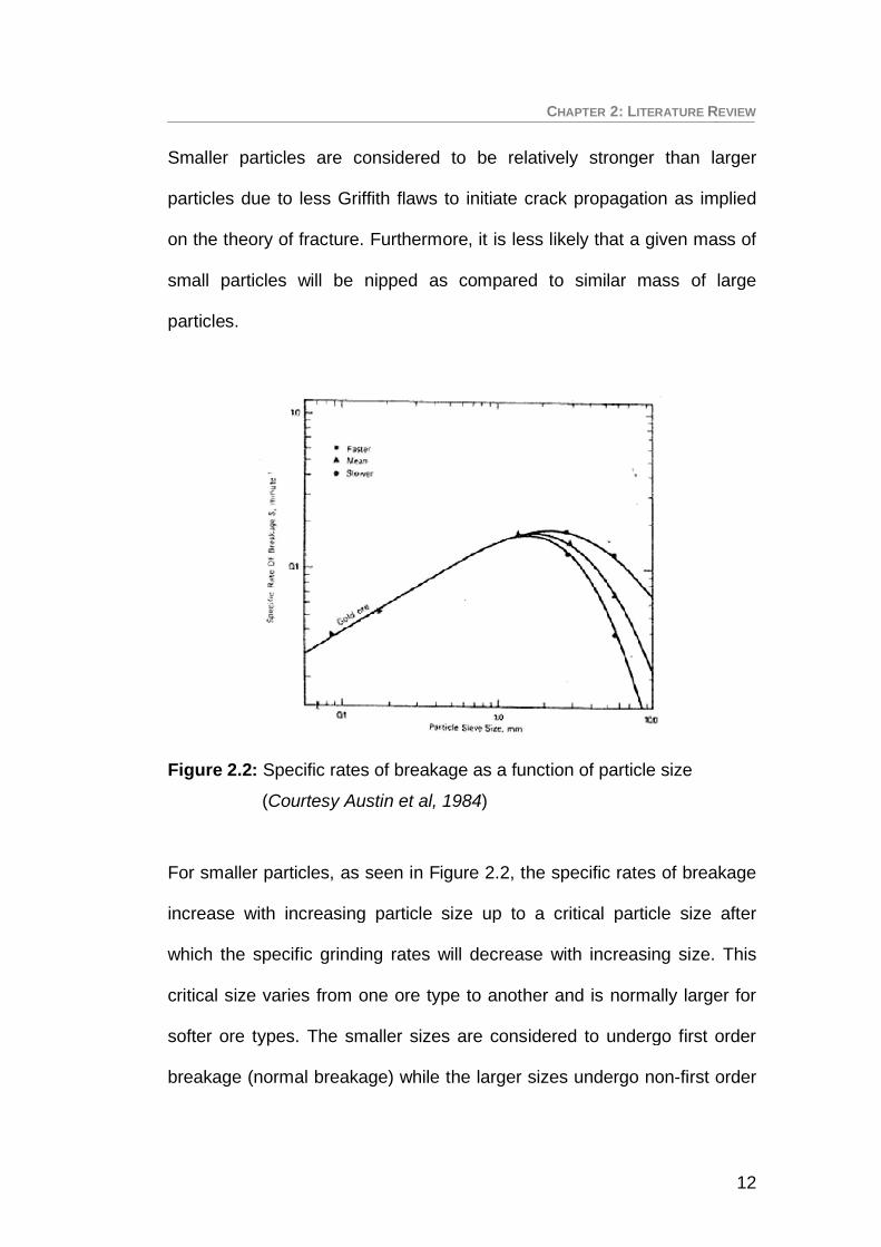
Smaller particles are considered to be relatively stronger than larger
particles due to less Griffith flaws to initiate crack propagation as implied
on the theory of fracture. Furthermore, it is less likely that a given mass of
small particles will be nipped as compared to similar mass of large
particles.
Figure 2.2: Specific rates of breakage as a function of particle size
(Courtesy Austin et al, 1984)
For smaller particles, as seen in Figure 2.2, the specific rates of breakage
increase with increasing particle size up to a critical particle size after
which the specific grinding rates will decrease with increasing size.
critical size varies from one ore type to another and is normally larger for
softer ore types. The smaller sizes are considered to undergo first order
breakage (normal breakage) while the larger sizes undergo non-first order
REVIEW
12
Smaller particles are considered to be relatively stronger than larger
particles due to less Griffith flaws to initiate crack propagation as implied
mass of
as compared to similar mass of large
For smaller particles, as seen in Figure 2.2, the specific rates of breakage
increase with increasing particle size up to a critical particle size after
which the specific grinding rates will decrease with increasing size. This
e ore type to another and is normally larger for
The smaller sizes are considered to undergo first order
first order

CHAPTER 2: LITERATURE R
breakage (abnormal breakage). In the case of abnormal breakage the
particle sizes are considered to be too big for the energy of the tumbling
balls to be used efficiently in causing fracture. The inclusion of lifters in a
mill and higher mill speeds tend to increase the rates of breakage of
coarse particles as a result of the increase of high energy impacts from
cataracting balls.
Figure 2.3: Specific rates of breakage as a function of particle and ball
filling (Courtesy Austin et al, 1984)
A low particle filling gives a small rate of breakage, as seen in Figure 2.3.
Increasing the particle filling will lead to the spaces between the balls
being filled and thus increasing the rates of breakage to a point where the
REVIEW
13
age the
be too big for the energy of the tumbling
fficiently in causing fracture. The inclusion of lifters in a
mill and higher mill speeds tend to increase the rates of breakage of
esult of the increase of high energy impacts from
Specific rates of breakage as a function of particle and ball
A low particle filling gives a small rate of breakage, as seen in Figure 2.3.
Increasing the particle filling will lead to the spaces between the balls
being filled and thus increasing the rates of breakage to a point where the

CHAPTER 2: LITERATURE REVIEW
14
void spaces are totally filled with particles (i.e. U=1). Increasing the particle
filling beyond this point will cause a decrease in the relative breakage rate
due to the fact that the collision zones are already saturated. Thus at a
given ball load it is undesirable to underfill or overfill a mill with particles. In
the case of low particle fillings (i.e. U<0.6) much of the energy is taken up
in steel to steel contact thus giving low values of volume of particles
broken per unit time per unit mill volume. Likewise steel on steel contacts
increase the chances of increased ball and liner wear. In the case of high
particle fillings (i.e. U>1.1) the particles cushion the breakage action thus
resulting in a low value of the volume of particles broken per unit time per
unit mill volume. In order to maximise the breakage rates for a specific ball
load an optimum particle filling of between 0.6 - 1.1 should be used.
Various techniques have been explored to measure the load behaviour
within a mill and are reviewed in detail below. Likewise, selected power
models and their basis of development are discussed.
2.1 LOAD BEHAVIOUR MEASUREMENT TECHNIQUES
The dynamic behaviour of the load can be measured either by mounting
the sensor directly onto the mill shell or mounting off the mill shell. On mill
sensors rotate with the mill and are able to provide continuously
information directly related to the condition of the mill charge at every point
on the mill. The challenges faced with this method include, effective

CHAPTER 2: LITERATURE REVIEW
15
methods of transmitting power and data from the sensor to a place off the
mill.
On-mill sensors that are placed in the mill through liner bolts (Vermeulen,
Ohlson and Schakowski, 1984) are always exposed to the harsh elements
within the mill and wear with time; variations in temperature within the load
can also cause a drift in the measurement made by the instrument. Such
factors that affect accurate and precise measurements have to be put into
consideration when calibrating the probes.
Off-mill sensors are normally fixed at one position close to the mill shell
and do not rotate with the mill. They monitor events related to conditions
within the charge indirectly as process variables are changed. With these
sensors it would be impossible to know the condition of the charge within
the mill. Through monitoring the events one can infer the conditions of the
mill that would lead to an efficient operation. A few techniques have been
reviewed below.
2.1.1 Acoustic Emission Measurement Technique
The grinding process in mills produces a lot of noise (acoustic emissions),
which depending on the conditions in the mill, can vary at different extents
of intensity. Experienced mill operators have been known to use this noise
to discern the load conditions within the mill. Acoustic emissions are
transient elastic waves within a material that are generated by an external

CHAPTER 2: LITERATURE REVIEW
16
stimulus such as mechanical loading. The acoustic emissions can provide
a measure of the characteristics of the charge or its motion within the mill.
In the past, microphones have been used to measure the sound intensity
generated from charge impacting onto the liners with the intention of using
this measurement in controlling industrial mill feed rates (Harding, 1939).
Here, the control philosophy would be the emptier the mill the noisier it is
and vice versa. Jaspan et al (1986) used multiple microphones to control
the pulp density and viscosity in a mill equipped with load cells and found
the system suitable for mill power draft maximisation and water addition
control. Recent interests in this area are analysing the acoustic emission
spectrum produced by mills subsequently relating it to mill control
variables (Watson, 1985). This involves the acquiring of data from a
microphone in time domain and converting it into frequency domain using
Fast Fourier Transforms (FFT). In frequency domain the spectrum
contains information related to the grinding process and mechanical
process occurring in a mill. Further analysis of this frequency spectrum is
done using a range of spectroscopic techniques. Pax (2001) preferred the
use of multiple sensors over a single sensor to acquire time domain data
due the sensors individually providing spatial information related to the
load condition at their location and likewise he was able to average the
coincident signals.
The challenge faced with acoustic emission measurement techniques is
that the analysis of the sound frequency spectrum must be able to isolate

CHAPTER 2: LITERATURE REVIEW
17
the frequencies due to the grinding process from other background
sources. The identification of the unique conditions of the charge prevalent
within the mill to the sound frequency spectrum is not straight forward and
more work has to be done. Any changes to the mill internals (i.e. liner
profile and grinding media shape) or operating conditions (i.e. wet or dry
mill, overflow or grate discharge, mill speed, ball filling etc) will have an
impact on the acoustic emission intensity. Thus the recalibration of the
sensor will have to be done to correct for these changes.
2.1.2 Conductivity Measurement Technique
This technique explores the use of the ability of the load to conduct an
electric current when the probe is in contact with the load. The technique
relies highly on the successful contact of the steel balls, wet autogenous
load or slurry with the probe’s assembled members. For a load comprised
of particles and balls in a dry mill, continuous current conduction between
the load and the probe is highly unlikely thus making the conductivity
probe not an attractive option for measuring load parameters in a dry mill.
Conductivity varies with temperature and should be kept in mind as the
probe shall experience drift in the value being measured as the load
temperature varies.
Moys (1985) pioneered the use of conductivity probes for analysing load
behaviour in a pilot ball mill. This probe was mounted into the mill and the
length of the probe’s sensing face was parallel to the mill axis. The long

CHAPTER 2: LITERATURE REVIEW
18
head of the probe allowed it to provide sharp changes in conductivity as it
enters and leaves the load. The probe was isolated from the bolt and
reinforcing channel by epoxy putty thus eliminating any chance of
electrical conductance between them (Figure 2.4). Successful continuous
contact between the balls, wet autogenous load or slurry and the probes
assembled members enabled a probe’s response.
Figure 2.4: Assembly diagram for the conductivity probe
For a ball only load, sharp changes were detected by the conductivity
probe at the toe and shoulder of the load. In the case of an autogenous
load, the rate of change in signal at the shoulder is governed by the rate at
which slurry drains of the probe and the slurry viscosity.

CHAPTER 2: LITERATURE REVIEW
19
At the University of the Witwatersrand a comprehensive study using
conductivity probes brought about an understanding of how the behaviour
of autogenous loads are affected by the slurry rheology, mill speed and the
load volume in a pilot mill (Smit, 2000). Furthermore, this technique has
been used in an industrial mill and conditions such as overloading,
premature centrifuging, off the grind and excessive slip were easily
detected by the conductivity probe (Moys, Van Nierop and Smit, 1996). In
this study premature centrifuging in the industrial mill occurred at the feed
end rather than the discharge end where it was expected that a higher
slurry percents solid would give rise to a high slurry viscosity. Not only has
this technique been used to measure load behaviour in ball or AG/SAG
mills but also in a HICOM nutating mill (Nesbit and Moys, 1998).
The conductivity measurement technique has not yet been developed into
a tool for mill control though it has proven itself in being able to provide
useful information that improves the understanding of load behaviour in a
mill. Measurements from the conductivity probe have been used to
improve mill power modelling capabilities which will lead to improved mill
control strategies and design (Van Nierop and Moys, 2001).
2.1.3 Vibrations Measurement Technique
Intense mechanical vibrations occur on the mill surface and machine
components attached to the mill mainly due to collision events occurring

CHAPTER 2: LITERATURE REVIEW
20
within a mill. The flexing of the mill shell and other external vibration
sources such as the drive motor, girth gear and surroundings also
contribute to mill vibrations. These later contributing factors are normally
assumed to be randomly distributed and give a constant contribution to the
mill vibrations. Thus process variables will mainly affect the occurrence of
collision events in the mill likewise the intensity of the vibrations. These
vibrations avail a good opportunity of discerning the mill condition as
affected by operating parameters through the use of accelerometers. An
accelerometer is an electromagnetic device that measures static or
dynamic acceleration forces. Accelerometers can either use the
piezoelectric effect or changes in capacitance to obtain an output signal
that varies with the intensity of the vibrations. Accelerometers can either
be attached on the mill shell or assemblies associated with the mill.
Similar to the acoustic emission technique, the vibration signal obtained in
time domain offers little information related to the condition of the charge.
It then becomes necessary to convert the signal into its frequency domain.
Vermeulen et al (1984) made use of piezoelectric sensors to measure mill
vibrations. Their novel technique of placing the sensor into a liner bolt
proved that physical information from within a mill could be continuously
obtained. Studies on laboratory scale (Zeng and Forssberg, 1992) and
industrial scale mills (Zeng and Forssberg, 1993) using accelerometers
mounted on bearings (i.e. the pinion bearing for the industrial mill)
revealed that the mill speed, powder filling, pulp density, pulp temperature

CHAPTER 2: LITERATURE REVIEW
21
and batch-wise grind time can be strongly correlated with a few frequency
bands in the power spectra. Similarly, Behera, Mishra and Murty (2007)
have made the use of accelerometers mounted on a bearing in a pilot mill.
Their signal processing method uses the amplitude of the dominant peak
obtained from a FFT spectrum and simply relates this to various mill
variables.
CSIRO (Commonwealth Scientific and Industrial Research Organisation –
Australia) patented the technique of using accelerometers fixed on the
moving surface of a mill to measure vibrations on industrial mills
(Campbell et al, 2003). In the various tests conducted on pilot and
industrial scale mills, they were able to calculate the toe and shoulder
positions of the load and compare them with actual photos of the load.
Important outputs from the system can also be used as soft sensors for
mill load and charge size though they are mill specific.
An interesting approach in this technique was the use of two
accelerometers mounted 180o apart on a mill shell coupled with the use of
a dynamic neural network (Gugel et al, 2003). The neural network acts as
a non linear classifier such that the current spectral signatures along with
other key parameters are used to output a fill level measurement for the
mill. The lack of proper training of the neural network to the various
vibration signatures as process variable are manipulated can lead to a
wrong output of the mill fill level.

CHAPTER 2: LITERATURE REVIEW
22
The challenge in this technique of load behaviour measurement lies in the
method that one uses to relate the frequency domain signal to the
conditions prevailing in the mill. The technique still holds much promise for
further research and industrial use.
2.1.4 Movement, Pressure or Force Measurement Technique
The forces exerted by the load on the liners can be resolved into
transverse and tangential forces. In order to measure the forces
independently the probe has to be designed such that it is able to resolve
the forces. Typically the probes will have a portion that is resident in the
mill (i.e. pressure plate, force plate or mill liner) so as to have a direct
contact with the load. The forces exerted by the load will be transmitted via
a thrust beam which is connected to a load beam. Mounted on the load
beam are strain gauges that are configured as a Wheatstone bridge and
connected to the appropriate circuits to provide the required output signal.
The movement probe will measure the resultant forces of the load on the
liners as the probe is not designed to measure the transverse or tangential
forces independently. The pressure or force probe both measure the
transverse forces exerted by the load on the liner. The value of this
measurement technique is that not only does it measure the load
behaviour it also gives a quantitative account of the forces exerted by the
load on a liner (Skorupa & Moys, 1993). These forces have a direct and
quantifiable effect on the wear mechanism and power drawn by mills.

CHAPTER 2: LITERATURE R
a) Section through a pressure probe for a pilot mill
b) Section through a improved variant of the pressure probe for a pilot mill
c) Section through a movement probe to be installed in an industrial mill
Figure 2.5: Illustrations of movement and pressure probes
REVIEW
23
for a pilot mill

CHAPTER 2: LITERATURE REVIEW
24
a) Industrial force probe assembly
b) Probe head designs c) Load beam
Figure 2.6: Force probe installed in an industrial mill
For load behaviour measurements the pressure probe exhibits a rapidly
rising response in its signal when it goes under the toe of the load but has
a poorly defined response for the shoulder position. This makes the probe
quite accurate and reliable in measuring the toe’s angular position.
Sensing steel plate
Shell boltStrain gauges
Amplifying circuit
Analogue Recording Module
Handheld module
To laptop

CHAPTER 2: LITERATURE REVIEW
25
Various designs of these probes can be seen in Fig. 2.5 & 2.6. Wits
University has dedicated a lot of time and resources in the improvement of
the pressure probe. One of the first designs of the pressure probe, which
was installed in a pilot mill, can be seen in Fig. 2.5a with subsequent
improvements leading to a new design to be used in wet mill is seen in
Fig. 2.5b. A force probe prototype for installation in industrial mills as seen
in Fig. 2.6 has been developed and tested in a coal mill of diameter 4.74m
and length 7.4m. Two different pressure plates (i.e. circular and square)
were tested (Fig. 2.6b). The thrust beam runs though a liner bolt and is
connected to the load beam (Fig. 2.6c) that seats outside the mill.
Tano et al (2005), reported of the development of a probe that is
influenced by the grinding charge motion and has the ability to collect
relevant information and used it for process control. The probe uses strain
gauges mounted inside rubber lifters. The sensor picks up the deflection of
the lifter when it moves through the grinding charge with a resolution of 1o.
Clear correlations between the signal profile and different charge
properties such as load volume, angle of repose and charge position exist
(Tano et al., 2005; Dupont and Vien, 2001b). The sensor has been
developed and integrated into a complete measurement system (Dupont
and Vien, 2001a) and was marketed by Metso minerals under the name of
Continuous Charge Measurement (CCM) sensor.

CHAPTER 2: LITERATURE REVIEW
26
The force measurement technique has also been applied to a Hicom
nutating mill using the tri-axial force sensor in Fig. 2.7 (Nesbit & Moys,
1998). The tri-axial force sensor measures the normal, tangential and axial
forces exerted by the load. Here the tri-axial force probe brought about an
understanding of the behaviour ball mass in the nutating mill.
Figure 2.7: Tri-axial force sensor installed in a Hicom nutating mill
2.1.5 X-ray Measurement Technique
This is a novel method developed at the University of Cape Town by
Powell and Nurick (1996a) that tracks the motion of balls deep within the
charge. Unlike other techniques that can either measure the balls at the

CHAPTER 2: LITERATURE REVIEW
27
periphery of the load or only the balls apparent at the end window of a mill
with this technique a more realistic and useful picture of the charge motion
can be obtained.
In order to overcome the challenges of viewing motion of balls deep within
the charge a bi-planar angioscope was used to film the ball motion using
an experimental Perspex mill. The bi-planar angioscope uses high energy
X-rays emitted in short pulses to stimulate a scintillating screen which are
then detected by a TV camera and relayed to an external monitor.
Permanent records are filmed in two planes simultaneously with cine
cameras resulting in a film of excellent resolution. Plastic beads were used
to make up the ball load with 4 opaque balls used for tracking. To track
rotation of a ball, one of the beads was fitted with a lead rod. The study
revealed several phenomena such as non-rotation of balls, charge dilation
that increases with mill speed, longitudinal migration of balls, insight into
charge segregation, spiralling action of balls and the smooth paths of balls
in the bulk of the charge. This technique can only be used for research
purposes and can be quite useful in obtaining experimental data that can
be used to verify the DEM model so that confidence can be given to its
predictive capabilities. Govender et al (2002) reported on an automated
3D mapping and space parameterisation technique of the images
obtained. Subsequently the accuracy has been further enhanced to be
able to track balls within 0.15mm (Govender et al, 2004).

CHAPTER 2: LITERATURE REVIEW
28
2.2 MODELS FOR MILL POWER
In milling, a feed of a known weight size distribution is to be milled to a
product of a finer weight size distribution at a desired rate of production.
The specification of the product size depends on the liberation
characteristics of the ore and the size requirements for optimal operations
of the downstream process. It is important to know the power requirements
to effect this size reduction and the corresponding size of the mill that
would carry out the duty. A commonly used method is to conduct
grindability tests (i.e. Bond’s Method) in a laboratory scale mill so as to
obtain the specific energy required to effect the required size reduction
and hence the industrial mill power can eventually be obtained. Various
power models and factors based on past experiences are then used to
calculate the overall size of the industrial mill. Another method is to use the
rates of breakage of a specific ore type or combination of ore types for a
known mill operating condition to determine the internal dimensions of the
mill. The power requirements for driving the mill are then obtained from the
internal dimensions by using a power model. This method accounts for the
breakage action in each size class and tracks the sizes and corresponding
masses through the mill. The method is appropriate for both mill design
and optimisation.
In the above methods for sizing mills it is important to have a good model
to either determine the power requirements of the industrial mill or to

CHAPTER 2: LITERATURE REVIEW
29
calculate the mill’s internal dimensions. Traditionally there have been two
major approaches used to develop mill power models. These are the
empirical approach (Rose & Sullivan, 1958; Bond, 1961b; Fuerstenau et
al, 1990; Moys, 1993 and Morrell, 1993) and the theoretical physics based
approach (White, 1905 and Mishra & Rajamani, 1992). The review of
power models will focus on the uniqueness of the load behaviour models
used by various researchers to develop their power models. It does not
serve as an exhaustive list of all power models proposed in literature.
2.2.1 Empirical Mill Power Models
The empirical approach approximates the shape of the load to be a
segment of a circle inclined a certain angle to the centre of the mill and
treats the load as a solid body (Fig. 2.8). In this case, the turning moment
of the frictional force balances the turning moment of the centre of gravity
of the bed around the mill’s centre. This method only accounts for the
energy required to raise the balls from the toe to the shoulder against
gravity. This approach does not account of energy recovered by the mill
shell due to cataracting balls striking it and also does not account for
internal friction of the load due to balls sliding over each other. The torque-
arm method calculates the mill’s torque (T) and power (P) using the
following models:
sin 2.1

CHAPTER 2: LITERATURE REVIEW
30
= 2.2
Where m is the mass of the load, g is the acceleration due to gravity; rc is
the radial distance from the centre of the mill to the centre of gravity, is
the angle of repose and N is the mill’s speed in rpm.
The general form for the empirical power models based on the torque-arm
approach is:
( ) ( ) ( ) ( ) ( ) ( ) 2.3
Where L is the load density, is the angle of repose, J is the load filling,
L is the mill’s length, D is the mill’s diameter and N is the mill’s speed.
In literature the diameter of the mill in power models is normally varies
exponentially with power and the exponent normally varies from 2.3 to 2.5.
The model assumes that the mill power is directly proportional to the mill’s
length and that the end walls of the mill have a negligible effect upon the
mill’s power. Further, it assumes that the tumbling action of the mill is
independent of the size of the mill provided that the ball diameter is much
less than the mill’s diameter.

CHAPTER 2: LITERATURE REVIEW
31
Figure 2.8: Illustration of the torque-arm load shape
An interesting alternative in describing the load shape for empirical power
models is the C-model proposed by Morrell (1993) and its variant the D-
model.
2.2.1.1 Rose and Sullivan’s Power ModelRose and Sullivan (1958) used the functional relations between
dimensionless groups, as seen in equation 2.4, to obtain a mill power
model for determining the net mill power for dry grinding as seen in
equation 2.5. The relationships between the various dimensionless groups
were obtained through experiments as dimensional analysis alone cannot
give a form of the relationships for these groups. In equation 2.4 the
functions enclosed in the first square brackets relate to the mill and ball

CHAPTER 2: LITERATURE REVIEW
32
load system while those in the second set of brackets relate to the
characteristics of the powder.
= ( ) ( ) ×
( ) ( ) 2.4
( )( ) 1 + ( ) 2.5
For equation 2.5, it is assumed that the mill’s net power is proportional to
the mill speed up to 80% of the critical beyond this the model cannot be
used. The term (1+ 0.4 U/ b) is a correction factor for the power to take
into account the powder tumbling with the balls. Here it is assumed the
powder occupied the void spaces between the balls at a certain particle
filling (U) and that the power is proportional to the weight of the balls plus
the powder. This correction factor holds for cases where the ratio of the
mill’s diameter to the particle diameter is less than about 400 or if the
particles are so small that segregation occurs. The empirically determined
function F(J) accounts for the effect of ball filling on the power. Rose and
Sullivan (1958) proposed the following parabolic function in equation 2.6
for ball fillings less than 50%.
( ) = 3.045 + 4.55 20.4 + 12.9 2.6

CHAPTER 2: LITERATURE REVIEW
33
The function was obtained by measuring the power drawn by a small
laboratory mill at known ball fillings. This function causes the maximum net
power drawn by a mill to occur at a ball filling of 40%.
2.2.1.2 Bond’s Power ModelBond’s (1961b) model which is the most widely accepted model was
obtained empirically by collating data from mills of various designs.
Equation 2.7 gives the power draw (P) for conventional ball mills using
make-up balls larger than one-eightieth of the mill’s diameter.
= sin( ) ( ) ( ) 2.7
Where K1 is a constant strongly affected by liner design and slurry
properties, L is the bulk density of the load, is the dynamic angle of
repose of the load, J is the ball filling fraction, L is the mill’s length, D is the
mill’s diameter and Nc is the mill speed expressed as a percentage of the
critical mill speed. B is a factor which is normally given the value of 0.937
and implies that the maximum power drawn by the mill would occur at a
ball filling of about 53%. The last factor in brackets accounts for the effect
of mill speed when close to the critical speed on the power drawn by the
mill. The parameters and normally have the value of 9 and 0.1
respectively. Bond’s model as seen in equation 2.7 treats all the variables
separately thus for example it does not allow for the fact that variations in

CHAPTER 2: LITERATURE REVIEW
34
the ball filling (J) affect the nature of the dependence of the mill’s power
draw on the mill’s speed.
2.2.1.3 Fuerstenau, Kapur and Velamakanni’s Power ModelFuerstenau et al (1990) studied the effects of polymeric grinding aids on
the grinding of dense slurries by changing the ball size, media charge,
mill’s speed and slurry holdup. Grinding in the presence of dense slurries
tends to cause the ball media to adhere to the mill wall and experience an
increase in cataracting or the balls are completely centrifuged. The
addition of polymeric dispersants tends to keep the load fluid and thus the
normal cascade – cataract behaviour dominates. To be able to describe
the effect of addition and non addition of polymeric dispersants on the
power in a ball mill a model which describes the load behaviour for both
cases had to be proposed.
The load shape model seen in Figure 2.9 attempts to describe the
dynamics (i.e. both cascading and cataracting) as well as a variable
partition of the charge between the two regimes as the pulp viscosity
changes with time. In this load behaviour model it is assumed that the
cataracting mass sticks uniformly on the mill shell and is lifted up before
dropping down on the cascading mass.

CHAPTER 2: LITERATURE REVIEW
35
Figure 2.9: Illustration of Fuerstenau et al simplified load shape
In drawing up the power model Fuerstenau et al (1990) considered the
power required by a mill to be the sum of the power drawn by the
cascading load (Pcs), the power drawn by the cataracting load (Pct) and
power due to a minor frictional component (Pf). The equations below give
a mathematical description of these power components:
Power drawn by cascading load (Pcs):
The cascading power can be drawn from any existing model. Fuerstenau
et al (1990) used the Hogg and Fuerstenau (1973) power model to
estimate the power drawn by the cascading charge.
= ( ) ( ) sin 2.8

CHAPTER 2: LITERATURE REVIEW
36
The function depends on the filling of the cascading fraction of the load
(J1) in the following manner:
( ) =( ), 0.35 < 0.5(1.05 1.33 ), 0.2 < 0.35 2.9
Where: N is the mill’s rotational rate (rpm), D is the mill’s internal diameter,
W is the mass of grinding charge, g is the acceleration due to gravity, J1 is
the ball filling of the cascading charge and is the angle of repose of the
load.
Power drawn by the cataracting load (Pct):
The power of the cataracting mass is estimated from the arced portion of
the load on the mill’s inner surface above the cascading load as illustrated
in Fig 2.7.
( ) sin + 2.10
= 2.11
[ ( )] 2.12

CHAPTER 2: LITERATURE REVIEW
37
Where: d is the ball diameter, W2 is the mass of cataracting charge, J is
the total mill filling, L is the mill’s length, is the load density, s is a time
dependent parameter that is a function of the slurry viscosity, X is a
function of the mill material system and is affected by addition of polymeric
dispersants and Z is a lumped parameter.
Power drawn by the minor frictional component (Pf):
This small power component is due to friction in the charge, its dilation,
slippage, de-mixing and percolation of particles in the voids between the
balls.
2.13
Where: C and K are constants.
Thus the power model can track the mills power draw as a function of
changing pulp viscosity with time, it permits estimations of the charge split
between the cascading and cataracting-centrifuging regimes of load
behaviour and also explains the occurrence of a peak torque value as the
slurry viscosity increases.
2.2.1.4 Moys Power ModelMoys (1993) developed a semi phenomenological power model based on
the understanding of the mill load behaviour. The load behaviour model,

CHAPTER 2: LITERATURE REVIEW
38
as seen in Fig. 2.10, is a compromise of the two extremes of load
behaviour that is a cascading load to cater for power draws at low speeds
and a centrifuging load component is introduced that caters for the
observed power loss as mill speeds increases. This simplification of the
mill load behaviour does not include the cataracting portion of the charge
but can account for the loss in power through cataracting balls striking the
exposed mill shell through its centrifuging load component. As a result this
model cannot give an indication of the fraction of load that is cataracting,
the onset of centrifuging or the thickness of the centrifuged layer.
Figure 2.10: Illustration of Moys simplified charge shape
Moys assumed that the power drawn by the active portion of the charge
was adequately described by Bond’s model and dropped out the term that
models the power as mill speeds nears 100% of the critical. When
substantial cataracting occurs coupled with a loss in power the centrifuged

CHAPTER 2: LITERATURE REVIEW
39
load model is activated and a portion of the load is assumed to be
centrifuged. This leads to a reduction in the mill’s effective diameter, mill
speed and likewise a reduction in the active load mass.
Thus the power model for a reduced active charge is given by:
sin 2.14
The effective diameter of the mill (Deff) is given by:
= ( ) 2.15
Here it is assumed that the thickness of the centrifuged layer is .
The effective mill filling (Jeff) is given by:
=( )
( )< 0.5[ ( ) ]
0, 0.5[ ( ) ]2.16
A simplification of equation 2.16 was proposed by Moys and its suitability
assessed. The simplification is:
= 20, 2 2.17

CHAPTER 2: LITERATURE REVIEW
40
A model that relates the thickness of the centrifuged layer to the mill’s
operating variables is seen in equation 2.18.
2.18
Where N* and N are parameters that are strong functions of liner profile
and slurry viscosity and J is a parameter that governs the strength of the
dependency of on the load filling J and will be a strong function of liner
profile.
For low mill speeds it is expected that no power loss will occur thus no
centrifuging ( = 0). As the speed is increased a drop in power begins
due to cataracting and at higher speed due to centrifuging this will
correspond with a rapid increase in . This phenomenon is reflected in the
exponential dependency of the mill’s speed (N) on . For a low mill filling,
minimal cataracting will be experienced if the liner allows substantial slip
and thus it is expected that = 0 but as the mill filling is increased and
slip reduced will become significant. If the liner does not allow for slip
then becomes independent of the load filling (J).
This proposed model does reflect the complex interactions of load volume
and speed on the power drawn by the mill. Certainly it could be quite
useful in determining the mill power drawn by South African style run-of-

CHAPTER 2: LITERATURE REVIEW
41
mine (ROM) mills as they are operated at high speeds at which liner profile
and slurry rheology have significant effects on the load behaviour. These
mills suffer from viscous slurry causing the grinding media to stick on the
liners causing premature centrifuging. Van Nierop and Moys (2001) used a
modified version of the Moys model to model an industrial AG mill’s power
after having insight into the nature of the load behaviour using conductivity
probes. The model could track the AG mill’s power quite well.
2.2.1.5 Morrell’s Power ModelThrough a photographic study of the evolving shape of a mill’s charge as
mill speed and charge filling increased for three liner profiles Morrell
proposed a new description of the charges shape as seen in Figure 2.11.
The crescent like shape was obtained through considering the portion of
the charge that exerts a force on the mill shell. The rest of the charge was
ignored by assuming that the cataracting portion has no direct effect on
the mill and that the eye of the load is stationary and of relatively small
mass thus having a negligible effect on the mill’s power draw. The
simplified charge description below was used to derive Morrell’s C power
model. The physical limits of the charge were defined by radial lines that
extend from the toe ( T) and shoulder ( Sh) to the mill’s centre, the charge
inner surface radius (ri) and the mill’s internal radius (rm). The physical
limitations of the charge had to be defined mathematically through
analysing the photographs of the load behaviour so that they would be
incorporated in the power model.

CHAPTER 2: LITERATURE REVIEW
42
Figure 2.11: Illustration of Morrell’s simplified charge shape
The mathematical descriptions are of the form:
Toe’s angular position ( T):
( ) + 2.19
Where A and B are parameters determined by regression analysis, c is
the experimentally determined critical speed and is the mill’s fraction of
critical speed.
Shoulder’s angular position ( S):
= ( ) 2.20

CHAPTER 2: LITERATURE REVIEW
43
Where E and F are parameters determined by regression analysis, T is
the shoulders angular position in radians and Jt is the mill filling.
Charge inner surface (ri):
2.21
Where rm is the mills internal radius and is an empirical model that is
defined as the fraction of charge bound by the toe, shoulder and charge
inner surface. It is assumed that was related to the time it takes for a
particle to move between the toe and shoulder within the charge and
between the shoulder and toe when in free flight.
Morrell derived his power model, seen in equation 2.22, using an energy
balance approach. The model considers the rate at which potential and
kinetic energy are generated within the charge.
=( )
{ ( 2)}{sin sin } +
( ){( ) ( 1) } 2.22
Where: = ( )
In its current form the model can only account for the power drawn by the
belly length of a mill and can be used only for grate discharge mills. To use
the model to approximate a wide range of industrial mill powers, Morrell

CHAPTER 2: LITERATURE REVIEW
44
further modified the model to account for power losses due to the
presence of a slurry pool in an overflow mill (equation 2.23) and the power
drawn by the charge in the conical ends of a mill (equation 2.24) and the
no load power (equation 2.25).
Net Power for the cylindrical section of an Overflow mill:
=( )
{ ( 2)}{sin sin } +
(sin sin ) +( )
{( ) ( 1) } 2.23
Where: = ( )
Net power for an overflow mill with cone ends (PC):
=( )
{ + 3 }{sin sin } + (sin sin ) +
( )+ 4 2.24
No load power (PNL):
= 2.62( ) 2.25
Where c is the density of the charge, Nm is the mills speed in rpm, rm is
the mill’s internal radius, ri is the radial distance from the mill’s centre to

CHAPTER 2: LITERATURE REVIEW
45
the charge inner surface, rt is radius of the trunnion and Ld is the length of
the conical end.
The C-model was applied to a database of 76 mills (38 ball mills, 28 SAG
mills and 7 AG mills) of various sizes and a wide range of power draws so
as to find the accuracy of its predictions. The C-model provided predictions
with a relative precision of 10.6% at the 95% confidence interval. Despite
the accuracies of this model one drawback for its application is the
complexity of the model and the number of empirical equations that are
required. Knowledge of the model form and its implementation has to be
sought in Morrell’s well documented thesis. Morrell’s model has further
been developed to a discrete shell model (D-Model) that is even more
complex than the C-model. The D-model attempts to approximate the
charge more realistically by sectioning the C-model into discrete shells so
as to represent the distinct layers present in the charge. Morrell chooses
the width of each of these discrete shells to be approximated by the
average particle size of the load. The physical boundaries of the D-model
are defined by equation 2.19, 2.20 and 2.21. The model has surely built its
reputation as a good model to predict industrial SAG/AG mill power draws.
2.2.2 Mechanistic Mill Power Models
Through the empirical load behaviour models illustrated in section 2.2.1
that are used to develop various power models it can be seen that they are
a gross simplifications of the actual load behaviour. Despite the models

CHAPTER 2: LITERATURE REVIEW
46
being easy to use they describe the load’s shape as a solid body thus not
reflecting the actual discrete nature of the load. The load behaviour
models fail to account for the recovery of energy by balls cataracting on to
the exposed mill shell thus they cannot be used as a diagnostic tool to
assess or optimise the ball or rock trajectories. The load behaviour models
are not capable of incorporating the effects of mill internals design (i.e.
lifter design, number of lifters, steel or rubber liners etc) on the load
behaviour. The importance of having a model that would treat the load as
discrete particles was realised quite early (White, 1905; Davis, 1919).
Furthermore models developed by McIvor (1983) and Powell (1991) try to
describe the influence liner profiles have on a single ball in the outermost
trajectory that is in contact with a liner.
2.2.2.1 The Discrete Element Method (DEM)The Discrete Element Method (DEM) was developed and applied to
granular material by Cundall and Strack (1979). The application of this
technique to studying the load behaviour in ball mills was done by Mishra
and Rajamani (1992) and has been a great benefit in the design and
optimisation of grinding mills.
The Discrete Element Method is a way of modelling the motions and
interactions of a set of individual particles and their environment as
affected by gravity, models for particle interaction and Newton’s laws of
motion. Collisions between particles are cleverly modelled by using the

CHAPTER 2: LITERATURE REVIEW
47
contact force law that consist of the linear spring, dashpot and slider as
seen in Figure 2.12.
Figure 2.12: Spring-slider-dashpot model for interactions between two
particles
The normal force is given by:
+ 2.26
The tangential force is given by:
{ , } 2.27
The particles are allowed to overlap by small amount ( x) typically
between 0.1- 0.5%. The normal (Vn) and tangential (Vt) relative velocities
determine the collision force by using the contact force law. The normal

CHAPTER 2: LITERATURE REVIEW
48
force has a linear spring that provides the repulsive force and dashpot to
dissipate a portion of the kinetic energy. The maximum overlap between
the particles is determined by the stiffness (kn) of the spring in the normal
direction. The normal damping coefficient (Cn) is chosen to give the
required coefficient of restitution ( ). The tangential force (Ft) model has an
integral term that represents an incremental spring that stores energy from
the relative motion of the particles and the elastic tangential deformation of
the contacting surface. The dashpot in the tangential force model
dissipates energy from the tangential motion and models the tangential
plastic deformation of the contact. The force is limited by the coulomb
frictional limit Fn at which the surface contact shears and the particle
begins to slide over each other. The structure of the DEM model can
further be coupled with Discrete Grain Breakage models (DGB),
Computational Fluid Dynamic (CFD), Smoothed Particle Hydrodynamics
(SPH) and Multi-Phase Flow models (MPF). Discrete Grain Breakage
models are used to define the breakage of particles in a comminution
device. Computational Fluid Dynamic models are used to compute the
fluid phase flow, interactions and transport within equipment. Smoothed
Particle Hydrodynamics is used to model non-Newtonian fluids such as
slurry as an assemblage of pseudo-particles with interactions related to
shear at any point in the slurry and provides a link between fluid transport
and fine particles in the slurry. Multi-Phase Flow models are used to model
particle and gaseous phases contained within the fluid.

CHAPTER 2: LITERATURE REVIEW
49
To account for the arbitrary particle shapes, sizes and density distributions
that are encountered in the mineral processing industry super-quadrics
can be used to define the particle.
The super-quadrics 3D geometric shapes are defined by the equation:
+ + = 2.28
Where: A, B and C represents the aspect ratio of the shape in its various
axes, S is the semi major axis of the shape and the power n determines
the angularity of the grinding media shape
The DEM requires intensive computing power especially when many
particles are involved and the level of complexity of the system being
modelled is high. The time required in simulating a full mill with balls,
rocks, slurry transport, rock breakage etc would take a couple of weeks on
a super computer or several months on a top of the range Pentium or
AMD desktop. Despite this the DEM is quite a versatile tool and has been
used to quantitatively predict the load behaviour (2D and 3D) in mills,
predictions of collision forces, energy spectra and power consumption
(Mishra and Rajamani, 1992 and Cleary, 1998); liner wear and its effect on
load behaviour (Kalala et al, 2007; Cleary, 1998 and Qui, 2001); Particle
breakage, grinding rates, liberation, and mill throughput (Cleary, 2001;

CHAPTER 2: LITERATURE REVIEW
50
Bwalya and Moys, 2003; and Potapov et al, 2007). Various mineral
processing equipment have been simulated with the intention of optimising
throughput through the equipment or just understanding the equipment
better. For this technique it is absolutely important to verify and test the
model against experimental results and not to perceive the simulation
results as reality. The lack of good experimental data for testing and
verifying DEM codes further limits the accuracy of the DEM predictions.
2.3 CONCLUSION
The basic purpose of milling of ores remains as a method of imparting
sufficient energy onto a rock to subsequently cause damage or breakage
of particles to some specified size distribution so as to expose the valuable
mineral for further downstream processes. Several measurement
techniques exist that are capable of measuring the extent of liberation from
a breakage action such as optical image analysers, scanning electron
microscopy analysers and x-ray micro-tomography analysers and have
improved in speed, accuracy and quality of information that one can
obtain. Depending on the mill’s operating conditions; a mill can contain a
wide range of breakage actions such as impact, chipping and abrasion.
Establishing the mode(s) of breakage that would lead to the optimum
damage and subsequent breakage of particles is the key in obtaining the
most efficient way of energy utilisation in any mill. Optimising the load
behaviour to target the mode of breakage required would be most

CHAPTER 2: LITERATURE REVIEW
51
important. Subsequently these broken particles need to be transported out
of the mill through a discharge mechanism with water or air acting as the
conveying agent. The discharge mechanism should also be designed in
such a way that it would encourage the exit of these particles out of the
mill. Discrete Element Method offers the best framework in which to carry
out such a study for an existing mill or when designing a new mill. Through
load behaviour measurement techniques one can then control the load
behaviour or use data from load behaviour measurements to calibrate a
DEM model.

CHAPTER3
MEASUREMENTTECHNIQUEMeasurement of the Load Behaviour in a Dry Pilot Mill
Using an Inductive Proximity Probe
Load behaviour in a dry pilot mill has been successfully measured as a
function of mill speed and load filling using an inductive proximity probe.
The inductive proximity probe detects the presence of metallic objects in
the proximity of its sensing face. Static and dynamic test demonstrate that
it is suitable for measuring load behaviour. The shoulder position is
measured more reliably by the inductive proximity probe due to this region
being well behaved and less variable as compared to the toe region. The
shoulder and toe angular positions of the inductive proximity probe signal
vary with mill speed and load filling. Cataracting of balls onto the mill shell
at high mill speeds is detected. The probe is sensitive to changes in mill
operating conditions and load packing. A comparison between the force
probe and the inductive proximity probe reveals that the inductive
proximity probe is superior in measuring load behaviour.
3

CHAPTER 3: MEASUREMENT TECHNIQUE
53
3.0 INTRODUCTION
Research into the load behaviour in grinding mills has been carried out to
give a better understanding of the effect various parameters (i.e. liner
profile, mill speed, mill loading etc) have on the load behaviour. This
insight can be used to optimise the load behaviour by using mill speed or
liner design, which can lead to significant improvements in production
capacity, energy efficiency and mill control. Vermeulen et al (1984) and
Moys (1985) showed that important information relating to the load
behaviour could be obtained from within a mill. The first ever reported
study on quantitative forces (radial and tangential) exerted by the load on
the liner as a function of operating variables of a pilot scale mill brought
about a better understanding of the load-liner interface interactions
(Skorupa and Moys, 1993). Powell & Nurick (1996a & 1996b) studied
particle motion in an experimental mill by using diagnostic x-rays from a bi-
planar angioscope. This novel method is an accurate technique for
tracking particle motion anywhere within the charge of a laboratory mill.
Kolacz (1997) successfully made use of strain transducers placed on the
mill shell to measure the mill load of a dry grinding industrial mill.
This research focuses on the use of an inductive proximity probe in
measuring the load orientation in a dry laboratory mill. The need to use the
inductive proximity probe in measuring load behaviour came about due to
the fact that the force probe measured earlier shoulder positions as

CHAPTER 3: MEASUREMENT TECHNIQUE
54
compared to a conductivity probe when used to measure load behaviour in
a wet environment (Moys, Smit and Stange, 1996). The probe can also
measure the behaviour of the steel balls independent of particles present
in the mill.
3.1 THE INDUCTIVE PROXIMITY PROBE
The inductive proximity probe is a solid state electronic device that detects
the presence of metallic objects at its sensing face. The probe’s principle
of operation is based on the induction coil. It is made up of a coil of copper
wire wound around a ferrite core, an oscillator, a detection circuit and an
output circuit. The oscillator circuit generates a fluctuating current through
the copper wire and induces a symmetrical, oscillating low energy electro-
magnetic field at the probe’s sensing face. When a metallic object moves
into this magnetic field, eddy currents are induced and begin to circulate
within the object. This eddy current magnetically pushes back and
dampens the probe’s magnetic field. The probe’s detection circuit monitors
this dampening effect and when the magnetic effect is sufficiently damped
the output circuit is triggered and gives an output.
A 30mm diameter inductive proximity probe with a measuring range of 3 –
8mm from its sensing face was used. A special housing was designed and
machined to support and mount the probe into the mill shell as seen in
Figure 3.1. The probe was mounted in the mill shell 50mm away from the

CHAPTER 3: MEASUREMENT TECHNIQUE
front plate. No side sensing of the metallic mill shell occurs as a result of
the probe being mounted into the mill shell. The 3mm PVC protection plate
bolted on the inside of the mill protects the probe’s sensing face from
impacts and abrasion caused by balls. A 6.4o angle is subtended by the
probe with the centre of the mill thus leading to an uncertainty of 3.2
the load behaviour measurements. The positioning of the probe relative to
the lifters will cause the shoulder’s angular position measurements to be
detected earlier than expected. This is due to the fact that balls depart
from the lifter last.
Figure 3.1: Inductive proximity probe’s assembly
The inductive proximity probe only detects the outer layer of balls close to
the mill shell in its 5mm sensing range from the surface of the PVC
ECHNIQUE
55
No side sensing of the metallic mill shell occurs as a result of
the probe being mounted into the mill shell. The 3mm PVC protection plate
ts the probe’s sensing face from
angle is subtended by the
3.2o on
the load behaviour measurements. The positioning of the probe relative to
the lifters will cause the shoulder’s angular position measurements to be
earlier than expected. This is due to the fact that balls depart
The inductive proximity probe only detects the outer layer of balls close to
the mill shell in its 5mm sensing range from the surface of the PVC

CHAPTER 3: MEASUREMENT TECHNIQUE
56
protection plate. Balls beyond this range are not expected to have any
influence on the signal.
3.2 EXPERIMENTAL EQUIPMENT AND METHOD
The mill used in these experiments has an internal diameter of 0.54m,
length of 0.15m and is equipped with 12 trapezoidal lifters each having a
height of 20mm and a 45o face angle. A front glass plate facilitated the
taking of still photographs and videos of the tumbling load. An inductive
probe and force probe were inserted into the mill. A marker signal made
up of an Infra-Red Light Emitting Diode, a spectrally matched
phototransistor and a 15mm wide mirror was aligned to the centres of all
probes. The inductive and marker signals were combined together to
produce a single signal. All signals were sent to a computer-based data
acquisition system via slip rings. The mill load comprised of a ball size mix
of 6, 7, 8, 9 and 10mm steel balls mixed together in equal proportions by
number. The mill filling was varied from 15 - 45% while the mill speeds
explored ranged from 60 – 105% of the critical mill speed.
3.3 INDUCTIVE PROXIMITY PROBE SIGNAL ANALYSIS
Preliminary test were conducted on the inductive probe so as to bring
about a better understanding of the type of signal that was expected from
the probe and to assess the probes suitability in measuring load

CHAPTER 3: MEASUREMENT TECHNIQUE
57
behaviour. In the first test a 30mm steel ball was moved across the
probe’s sensing surface at a distance of 0 to 8mm away from the surface.
The grey shaded area in Figure 3.2 indicates the distance covered by the
PVC protection plate and the area shaded yellow represents the probe’s
measuring range.
Figure 3.2: Inductive proximity probe’s static response curves for a 30mm
steel ball at various distances away from the probe’s centre.
As the steel ball approaches the probe; the probe’s signal drops from a
high voltage to a low voltage. The extent of the drop in the signal is
affected by the objects shape, size, material and position within the
sensing range. The signals obtained from the centre and at a distance of
7.5mm away from the probe’s axis vary linearly with an increase in
distance of the steel ball away from the probe’s sensing face. At a distance

CHAPTER 3: MEASUREMENT TECHNIQUE
58
of 15mm away from the probe’s centre the steel ball was not detected in
the measuring range. The next test characterised the probe’s response to
a dynamic stimuli. A steel plate 5mm thick was placed on top of the probe
and a steel rod was used to knock it off. Figure 3.3 represents the probe’s
response.
Figure 3.3: Dynamic response of the inductive proximity probe.
The time it takes the signal to rise to 98% of its final value (t98) was 6.9ms.
This rise time causes an error of 2.54o on the load behaviour
measurements at the highest speed (i.e. 60.87rpm). The time constant ( c)
was 2.8ms.
0
10
20
30
40
50
60
70
80
90
100
0.096 0.098 0.1 0.102 0.104 0.106 0.108 0.11Time (sec)
Indu
ctiv
e Pr
oxim
ity P
robe
's R
espo
nse
(%)
t98 = 6.1ms
c = 2.8ms

CHAPTER 3: MEASUREMENT TECHNIQUE
59
3.3.1 Description of the Inductive Proximity Probe’s Signal
In Figure 3.4 a typical signal for five mill revolutions (data points) and the
average signal of the five mill revolutions (solid line) for a load filling of
35% and mill speed 75% is presented. The different regions of the load
behaviour in the photograph and that of the signal from the inductive probe
are labelled. An analysis of the bulk toe and shoulder for each individual
revolution can be seen in Table 3.1. The load behaviour signals are
relatively regular shaped and reproducible for each mill revolution. Impacts
prior to the bulk toe are detected between the 90-120o angular position this
is due to balls jumping in and out of the toe region. The data from each
individual revolution in the toe region (i.e. between 120-160o) show a lot of
scatter and a variable drop in the average signal. This occurs as a result of
the balls continuously rearranging themselves and trying to pack
themselves so as to attain the smallest possible voidage. As balls pack
better and are locked into circular paths that move with the same angular
velocity of the mill shell (i.e. between 160-290o) the average signal tends
to become less variable and the data points from individual revolutions
exhibit less scatter. The variation in the signals of some individual
revolutions is a result of the ball packing not being the same during each
revolution. The rising signal in the shoulder region for individual revolutions
as well as the average signal (i.e. between 290-310o) are less scattered as
compared to the signal in the toe region.

CHAPTER 3: MEASUREMENT TECHNIQUE
60
Figure 3.4: Typical signal from the inductive proximity probe for a mill
filling of 35% and a mill speed of 75% of the critical mill speed
Table 3.1: Bulk toe, Load locked in and Shoulder angular positions for a
mill filling of 35% and a mill speed of 75% of the critical
MillRevolution
Upper Threshold Lower Threshold
Bulk Toe(Degrees)
Shoulder(Degrees)
Load Locked in(Degrees)
Shoulder(Degrees)
1 125.3 308.4 157.2 294.9
2 119.5 309.3 159.8 292.2
3 125.8 307.0 168.0 294.2
4 126.7 310.0 152.1 295.8
5 129.0 308.7 165.1 294.5
Average 125.3 308.7 160.4 294.3
StandardDeviation 3.5 1.1 6.3 1.3

CHAPTER 3: MEASUREMENT TECHNIQUE
61
To process the raw data obtained from the inductive probe meaningfully
one has to clearly define the different regions of the load as detected by
the inductive proximity probe. Upper and lower thresholds were chosen to
analyse the signals obtained as seen in Figure 3.4. The following regions
were then defined:
Impact toe: This is the part of the signal where the probe first comes in
contact with steel balls. It is labelled as B in Figure 3.4. There is an abrupt,
momentary drop in the signal and then it instantly returns to its original
high-level voltage state of non-metal detection. It is located just before the
bulk toe although for higher mill speeds it is detected much earlier than the
bulk toe due to cataracting balls impacting on the down coming side of the
mill shell.
Bulk toe: This is the portion of the signal where it drops continuously from
its high-level voltage state of non-metal detection eventually reaching the
low-level voltage state of the signal. It is labelled as C in Figure 3.4. The
upper threshold is used to obtain a quantitative measure of the bulk toe.
Load locked in: This is the point just before the variable dropping signal
reaches its low-level voltage state. It is obtained from the lower threshold.
It is labelled as D in Figure 3.4.
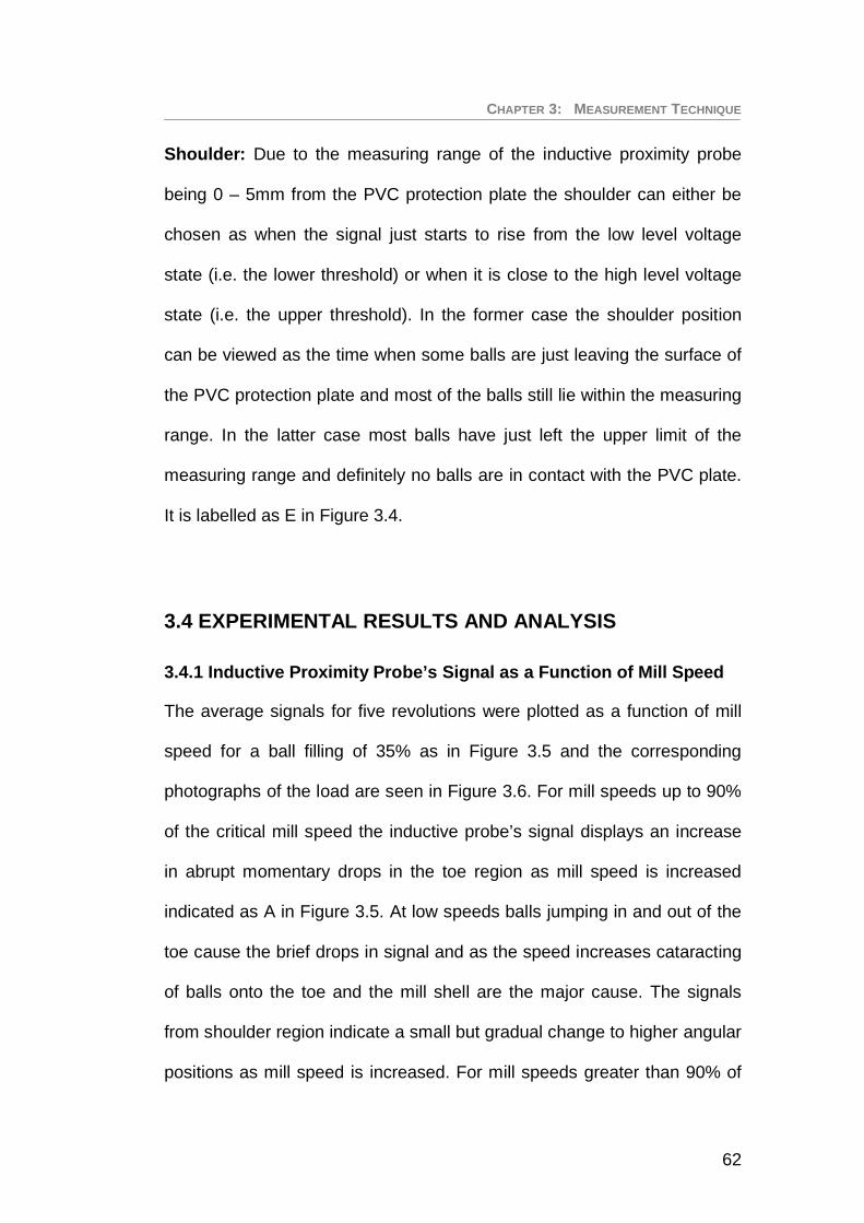
CHAPTER 3: MEASUREMENT TECHNIQUE
62
Shoulder: Due to the measuring range of the inductive proximity probe
being 0 – 5mm from the PVC protection plate the shoulder can either be
chosen as when the signal just starts to rise from the low level voltage
state (i.e. the lower threshold) or when it is close to the high level voltage
state (i.e. the upper threshold). In the former case the shoulder position
can be viewed as the time when some balls are just leaving the surface of
the PVC protection plate and most of the balls still lie within the measuring
range. In the latter case most balls have just left the upper limit of the
measuring range and definitely no balls are in contact with the PVC plate.
It is labelled as E in Figure 3.4.
3.4 EXPERIMENTAL RESULTS AND ANALYSIS
3.4.1 Inductive Proximity Probe’s Signal as a Function of Mill Speed
The average signals for five revolutions were plotted as a function of mill
speed for a ball filling of 35% as in Figure 3.5 and the corresponding
photographs of the load are seen in Figure 3.6. For mill speeds up to 90%
of the critical mill speed the inductive probe’s signal displays an increase
in abrupt momentary drops in the toe region as mill speed is increased
indicated as A in Figure 3.5. At low speeds balls jumping in and out of the
toe cause the brief drops in signal and as the speed increases cataracting
of balls onto the toe and the mill shell are the major cause. The signals
from shoulder region indicate a small but gradual change to higher angular
positions as mill speed is increased. For mill speeds greater than 90% of

CHAPTER 3: MEASUREMENT TECHNIQUE
63
the critical mill speed distinct drops in the inductive proximity probe’s
signal are detected close to the 60o angular position (indicated as B in
Figure 3.5); this is caused by cataracting balls impacting on the mill shell.
Figure 3.5: Inductive probe’s signal as a function of mill speed for a load
filling of 35%
This sort of behaviour is also reflected in Figure 3.6 for mill speeds of 95%,
100% and 105%. The signal from the shoulder region becomes less steep
at high speeds and covers a wider angular range. After the balls in contact
with the PVC plate and within the measuring range of the inductive probe
are projected into space they follow a trajectory that lies within the probe’s
measuring range and travel a wider angular range before leaving the
upper limit of the probe’s measuring range. This behaviour is clearly

CHAPTER 3: MEASUREMENT TECHNIQUE
64
reflected by comparing the balls in the shoulder region in Figure 3.6 as mill
speed is increased.
Mill speed = 60% of criticalspeed
Mill speed = 70% of criticalspeed
Mill speed = 75% of criticalspeed
Mill speed = 80% of criticalspeed
Mill speed = 85% of criticalspeed
Mill speed = 90% of criticalspeed
Mill speed = 95% of criticalspeed
Mill speed = 100% ofcritical speed
Mill speed = 105% ofcritical speed
Figure 3.6: Photographs of the load behaviour as a function of mill speed
for a load filling of 35%

CHAPTER 3: MEASUREMENT TECHNIQUE
65
3.4.2 Inductive Proximity Probe’s Signal as a Function of Mill Filling
The average signals for five revolutions were plotted as a function of ball
filling at 75% of the critical mill speed. The average signal at low mill
fillings (J = 15%) is noisier than signals for higher mill fillings (J > 25%) as
seen in Figure 3.7.
Figure 3.7: Inductive proximity probe’s signal as a function of mill filling for
a mill speed of 75% of the critical mill speed
This is due to the pressure exerted by the mill load on the liner being low
thus causing the balls to loosely slide over the probe’s sensing surface
thus causing fluctuations in the signal. For higher mill fillings the inductive
0
5
10
15
20
25
30
35
40
0 30 60 90 120 150 180 210 240 270 300 330 360Angular Position (Degrees)
Indu
ctiv
e Pr
oxim
ity P
robe
's R
espo
nse
(Vol
ts -
grap
hsar
e su
cces
sive
ly tr
ansl
ated
by
10V)
15%
25%
35%
45%Ball Filling

CHAPTER 3: MEASUREMENT TECHNIQUE
66
proximity probe’s signal at the toe region is less noisy than that of low mill
fillings. This is due to the charge surface forming a tri-linear saddle shape
as explained by Dong and Moys (2003). This shape of the charge causes
more balls to be consolidated at the toe region therefore improving their
packing at high mill fillings despite the turbulent nature of the toe region as
seen in Figure 3.8. The shoulder position moves to higher angular
positions as mill filling is increased.
Load filling = 15% of mill volume Load filling = 25% of mill volume
Load filling = 35% of mill volume Load filling = 45% of mill volume
Figure 3.8: Load behaviour as a function of load filling for a mill speed of
75% of the critical mill speed.

CHAPTER 3: MEASUREMENT TECHNIQUE
67
3.4.3 Load Orientation as a Function of Mill Speed and Mill Filling
The load orientation as a function of mill speed and filling is represented in
Figure 3.9. The error bars represent 1 standard deviation calculated
from the measurements of the toe and shoulder positions of five mill
revolutions. The toe of the load remains relatively constant up to 90% of
the critical mill speed after which it moves rapidly to lower angular
positions. This is due to the increased cataracting of balls onto the mill
shell close to the toe region at high mill speeds.
Figure 3.9: Load orientation as a function of mill speed and filling
measured by the inductive proximity probe
The toe position for higher mill fillings is at a lower angular position than
that of lower mill fillings. The shoulder of the load increases gradually to
higher angular positions as mill speed is increased to 90% of the critical
0
30
60
90
120
150
180
210
240
270
300
330
360
50 55 60 65 70 75 80 85 90 95 100 105 110
Mill Speed (% of critical mill speed)
Ang
ular
Pos
ition
(Deg
ree)
J = 15% J = 25% J = 35% J = 45%
Bulk Toe
Shoulder

CHAPTER 3: MEASUREMENT TECHNIQUE
68
mill speed due to more lift being imparted to the load as mill speed is
increased. At speeds greater than 90% of the critical mill speed the
tendency of the load to start centrifuging causes the shoulder position to
move rapidly to higher angular positions. The shoulder’s angular position
is higher for higher mill fillings than for lower mill fillings, and the toe
position is earlier. Higher mill fillings tend to result in cataracting earlier
than low mill fillings.
3.4.4 Comparison of the Inductive Probe with the Force Probe
An experiment was performed so as to obtain a comparison between a
force probe that measures the radial forces exerted by the load on the mill
shell and an inductive proximity probe. The results of this experiment can
be seen in Figure 3.10 and a quantitative analysis in Table 3.2. The ball
filling was 15% and the mill was run at 75% of the critical mill speed. The
toe position of the force probe signal was obtained by assuming it to be
the point where there is an evident sudden increase in the force signal and
the shoulder position was determined as the intersection of a two straight
lines fitted to the decreasing force signal and the no load force signal as
described by Moys, Smit and Stange (1996).The force probe measured
the location of the shoulder of the load earlier than the inductive proximity
probe. In this case it is actually at an angular position 12.6o earlier than
that measured by the inductive proximity probe at the lower threshold ( sh,
Ind, 2) and 27.4o earlier than that measured at the upper threshold ( sh, Ind, 1).

CHAPTER 3: MEASUREMENT TECHNIQUE
69
Figure 3.10: Inductive proximity and force probe signals for J = 15% and
N = 75%
Table 3.2: Analysis of the inductive and force probe signals for five
revolutions for J = 15% and N = 75%Inductive Proximity Probe Force ProbeUpper Threshold Lower Threshold
Mill Revs. BulkToe Shoulder Load
Locked In Shoulder BulkToe Shoulder
1 138.8 296.0 185.8 279.8 142.8 270.92 145.5 298.8 178.8 282.6 134.3 264.03 147.2 296.0 181.9 280.6 142.0 268.64 149.0 295.6 179.2 284.0 142.8 270.95 147.6 298.2 177.7 283.5 141.3 273.2
Average 145.6 296.9 180.7 282.1 140.6 269.5StandardDeviation 4.0 1.5 3.2 1.8 3.6 3.5
The force probe cannot measure the shoulder position accurately because
at angular positions greater than 270o the balls in contact with the force
probe exert little or no radial force and are held in contact with the force

CHAPTER 3: MEASUREMENT TECHNIQUE
70
probe by their own momentum and support from balls below. Thus the
inductive proximity probe is more suitable than the force probe in
measuring the shoulder’s angular position. A 5o difference is seen between
the measurements of the toe position from both probes. The force probe
registers an earlier toe as compared to the inductive proximity probe.
3.5 CONCLUSION
An inductive proximity probe was employed in this study and has been
shown to be suitable in measuring the load orientation within the mill as a
function of operating conditions prevailing. A reliable measure of the
shoulder position can be obtained from the inductive proximity probe due
to the well-behaved nature of this region as compared to the toe region,
which is a turbulent and variable region. Direct impacts onto the mill shell
by the cataracting balls were also detected. The load lock-in position can
also be located. Comparisons between the inductive proximity probe and
the force probe reveal that inductive probe is superior in measuring the
shoulder position. The nature of the signal from the inductive probe for
different mill speeds and fillings differ. A change in ball packing and the
tendency of the load to slip at low mill fillings is also detected. This shows
that the probe is sensitive to changes in operating conditions prevailing in
the mill and also changes in load structure.

CHAPTER4
EXPERIMENTAL STUDYParticle filling and size effects on the ball load behaviour and power
in a dry pilot mill: Experimental Study
The ball load behaviour in a pilot mill is studied under conditions of
increasing particle filling, for coarse silica feed (0.8-1.8mm) and fine silica
feed (0.075-0.3mm), at the mill speeds of 63, 78, 88 and 98% of the
critical. An inductive probe is used to obtain the ball load behaviour
independent of particles present in the mill. The difference in mill power
draw obtained from the coarse and fine particle charges are explained via
their load behaviour signals. The effect of particle filling and size on the
ball load behaviour is quantified through the toe and shoulder angular
positions. Radial segregation of the coarse silica particles to the periphery
of the charge occurs. A radial segregation index related to the extent of
drop in the inductive probe’s signal has been defined and used to quantify
radial segregation as a function of particle filling and mill speed.
4

CHAPTER 4: EXPERIMENTAL STUDY
72
4.0 INTRODUCTION
Ball mills are typically operated close to their maximum power draw. At the
maximum power draw, it is assumed that the ball charge is well mixed and
void spaces between the balls are filled with particles. But, in reality,
particles can influence the ball charge in various ways causing the
maximum power draw to shift depending on the nature of the influence.
The ball load contributes to the bulk of the charge mass; consequently a
change in the location of its centre of gravity significantly affects the power
drawn by the mill. It is therefore worthwhile to study the behaviour of the
ball charge and the influence particles have on it. From such a study, one
can infer the conditions within the charge that lead to maximum power
draw and optimal throughput.
Several intrusive and non-intrusive techniques have been developed to
measure the dynamic behaviour of a mill’s charge in order to improve the
understanding, optimisation and control of mills. These techniques include
strain (Kolacz, 1997; Tano et al, 2005), acoustic emissions (Pax, 2001),
vibration (Zeng & Forssberg, 1992; Campbell et al, 2001; Behera et al,
2007), x-rays (Powell & Nurick, 1996a & 1996b), conductivity (Moys,
1985), force (Moys & Skorupa, 1993) and inductivity (Kiangi and Moys,
2006). The following study uses a novel technique that measures ball load
behaviour with an inductive proximity probe. The probe has been shown to
be capable of obtaining useful information directly related to the ball load

CHAPTER 4: EXPERIMENTAL STUDY
73
behaviour in a pilot mill (Kiangi and Moys, 2006); including an industrial
mill (Dong et al, 2005). It’s intended use however, is not to be developed
as a tool for mill control, but rather to be used to obtain useful information
that can help one better understand the ball load behaviour and the
variables that affect it. This chapter presents an experimental study of the
effect that both particle filling and size have on the ball load behaviour and
net power in a dry batch pilot mill.
4.1 EXPERIMETAL EQUIPMENT AND METHOD
A mill of diameter 0.526m and length 0.18m was used (Figure 4.1a). The
mill rotates in an anticlockwise direction i.e. in the direction of increasing
angular displacement. The mill was fitted with 24 trapezoidal lifters, each
with a height of 5mm and a face angle of 45o. The lifters are scaled down
versions of Eskom’s Matimba power station’s worn liners. The ball load
was filled to 20% (36.08kg) of the mill’s internal volume, similar to that
found in Eskom’s coal mills and comprised of 6,7,8,9 and 10mm balls
mixed together equally in number. The inductive probe was placed
between two lifters 20mm from the front end plate and a grey PVC
protection plate was bolted on the inside of the mill over the probe’s
sensing surface so as to protect the probe from the harsh conditions
prevailing in the mill (Figure 4.1b). The probe senses the presence of steel
balls within a 5mm range from the surface of the PVC protection plate (i.e.
equivalent to the height of the lifters). As a result, the inductive probe could

CHAPTER 4: EXPERIMENTAL STUDY
74
only sense balls in the outer 5mm layer of the charge in contact with the
mill shell. The net torque was measured via a calibrated load beam after
subtracting the mill’s no-load torque from the gross torque obtained.
a) Photograph of the mill and axis of orientation of the load
b) Inductive probe installation on the mill
Figure 4.1: Photograph of the mill and the installation of inductive
proximity probe.
Silica sand with a bulk density of 1480kg/m3 was used as feed material.
The coarse silica sand particle size was 0.8-1.8mm (50% passing
0o (360o)
90o
180o
270o
0o (360o)
90o
180o
270o

CHAPTER 4: EXPERIMENTAL STUDY
75
1102 m) as seen in Figure 4.2a and the fine silica sand particle size was
0.075-0.3mm (50% passing 173 m) as seen in Figure 4.2b. The silica
sand was coned, quartered and riffled in order that a representative feed
sample could be obtained. Particle filling was defined as the fraction of
void spaces within the resting ball load that are filled with particles. Coarse
particle fillings of 20-150% (0.92-6.87kg) and fine particle fillings of 20-
160% (0.92-7.33kg) were used during experimentation.
a) Coarse particles b) Fine particles
Figure 4.2: Photographs of the coarse and fine particles
For each particle filling, four different mill speeds were used; they were
varied from 63-98% (37-57.6rpm) of the critical. The inductive probe and
load beam signals were sampled for each particle filling and mill speed
used. The sampling time for each particle filling at a specific mill speed
was 22.6s which yielded about 10 to 13 mill revolutions at the lowest
speed used. The signals were sampled twice per degree at the highest mill
speed used and translated to a sampling frequency of 708Hz. Consecutive

CHAPTER 4: EXPERIMENTAL STUDY
76
particle fillings were attained by adding fresh silica onto the charge
containing ground silica sand from the previous particle filling. The total
grinding time for the coarse and fine particle experiments were about 15
minutes each. Performing the experiment in this manner would lead to an
increasing amount of fines generated within the load as particle filling is
increased. The particle size distribution at the end of the experiments was
50% passing 711 m for coarse particles and 50% passing 61 m for fine
particles. It was deemed reasonable to perform a short experiment at a
single speed so as to reduce the extent of change in particle size
distribution as particle filling is increased and deduce the effect it has on
load behaviour and power.
4.2 RESULTS AND DISCUSSIONS
The data yielded various power curves, which are analysed below with
respect to their corresponding load behaviour signals. All power and load
behaviour signals plotted for each individual particle filling at a specific
speed are an average of ten mill revolutions. Additionally, error bars
included in graphs represent one standard deviation from the average
value.
4.2.1 Effect of particle filling and particle size on the net power
There is a notable difference in the variation of net power with increasing
particle filling for both coarse and fine particles as illustrated in Figure 4.3.

CHAPTER 4: EXPERIMENTAL STUDY
77
For coarse particle fillings at 63% of the critical speed (Figure 4.3a), the
power increases gradually as particle filling is increased to 150%.
Increasing the mill speed to 78% of the critical causes the mill power to
peak between the particle fillings of 70-110%. Further increasing the mill
speed shifts the peak power to lower particle fillings between 40-70% for
88% of the critical speed and between 20-60% for 98% of the critical
speed. A rapid decrease in the power is experienced following the peak in
power for 78, 88 and 98% of the critical speed. Mills are operated close to
where the peak power occurs and at this power it is assumed that the void
spaces between the balls are fully occupied with particles. If the maximum
power drawn shifts to lower particle fillings as the mill speed increases it
can cause increased ball and liner wear rates for that period of operation
as they will be fewer particles present in the mill at high mill speeds than at
low mill speeds.
a) Coarse particles b) Fine particles
Figure 4.3: Variations in net power draw with particle filling at different mill
speeds for a ball filling of 20%.
100
150
200
250
300
350
0 10 20 30 40 50 60 70 80 90 100 110 120 130 140 150 160Particle Filling (%)
Pow
er (W
atts
)
63%
78%
88%
98%
Mill Speed
Coarse Particles
100
150
200
250
300
350
0 10 20 30 40 50 60 70 80 90 100 110 120 130 140 150 160Particle Filling (%)
Pow
er (W
atts
)
63%
78%
88%
98%
Mill Speed
Fine Particles

CHAPTER 4: EXPERIMENTAL STUDY
78
For the fine particle curves (Figure 4.3b), the power drawn at 63, 78 and
88% of the critical speed are relatively flat compared to those obtained for
the coarse particles (Figure 4.3a). Additionally, the peak in power for the
fine particle filling occurs between particle fillings of 80-110%. At the mill
speed of 98% of the critical, the peak power shifts to lower particle fillings
between 20-40% and rapidly drops at higher particle fillings. Similar results
have been found where the maximum power draw occurs when the
powder filling fraction is about 0.6 and 0.5 for rod and ball mills
respectively (Zeng & Forssberg, 1991). Likewise, in a wet mill where the
net mill power depends on the slurry concentration and powder filling there
is an optimum powder filling for each slurry concentration that gives a
maximum in power (Tangsathitkulchai, 2003).
4.2.2 Effect of particle filling and particle size on the ball loadbehaviour
Figure 4.4 illustrates the inductive probe’s signal and ball load orientation
as a function of particle filling at a mill speed of 63% of the critical. The
load behaviour signals for each particle filling are translated by one volt
along the probe’s response axis so as to improve their visibility (Figure
4.4a and 4.4c).Vertical dotted lines indicate the toe and shoulder angular
positions for the ball-only load. Addition of coarse particles to the ball load
causes a gradual rise in the shoulder’s angular position from 280o to 297o
(Figure 4.4b). The power at this mill speed rises continuously despite the
charge’s density dropping at particle fillings greater than 100%. A rise in

CHAPTER 4: EXPERIMENTAL STUDY
79
the shoulder’s angular position from 280o to 295o is experienced with
increasing fine particle filling (Figure 4.4d). For fine particles the power
drops slightly after a particle filling of 90% despite the shoulder’s angular
position rising to 295o. In both cases, the toe’s angular position remains
constant. In the inductive probe’s response for coarse particles (Figure
4.4a), the voltage drop changes gradually from 5.5V for the ball-only load
to 4.8V at a particle filling of 110%.
a) Inductive probe signal - coarse particles c) Inductive probe signal – fine particles
b) Load orientation and Power – coarseparticles d) Load orientation and Power – fine particles
Figure 4.4: Inductive probe’s signal, ball load orientation and Power draw
as particle filling increases at 63% of the critical speed for a
ball filling of 20%.
-2-10123456789
10111213141516
0 30 60 90 120 150 180 210 240 270 300 330 360Angular Position (Degrees)
Prob
e's
Res
pons
e (V
olts
)
0%20%40%60%70%80%90%100%110%150%
Particle Filling
Toe for ball-only loadShoulder for ball-only load
5.5V
3.75V
4.8V
Coarse Particles, N63%, J20%-2-10123456789
10111213141516
0 30 60 90 120 150 180 210 240 270 300 330 360Angular Position (Degrees)
Prob
e's
Res
pons
e (V
olts
)
0%20%40%60%70%80%
90%100%110%120%160%
Particle Filling Toe for ball-only loadShoulder for ball-only load
5.5V
5.2V
Fine Particles, N63%, J20%
0
30
60
90
120
150
180
210
240
270
300
330
360
0 10 20 30 40 50 60 70 80 90 100 110 120 130 140 150 160Particle Filling (%)
Ang
ular
Pos
ition
(Deg
rees
)
0
30
60
90
120
150
180
210
240
270
300
330
360
Pow
er (W
atts
)
Shoulder
Toe
Power
Coarse Particles, N63%, J20%
0
30
60
90
120
150
180
210
240
270
300
330
360
0 10 20 30 40 50 60 70 80 90 100 110 120 130 140 150 160Particle Filling (%)
Ang
ular
Pos
ition
(Deg
rees
)
0
30
60
90
120
150
180
210
240
270
300
330
360
Pow
er (W
atts
)Shoulder
Toe
Power
Fine Particles, N63%, J20%

CHAPTER 4: EXPERIMENTAL STUDY
80
A further increase in the particle filling to 150% leads to a substantial
voltage reduction to 3.75V. Most likely radial segregation is occurring
within the coarse particle charge. Here, the particles are preferentially
segregated to the periphery of the load in contact with the mill shell. To
determine radial segregation, a comparison of the extent in voltage drop
from signals obtained in a ball-only load versus a combined ball-particle
load was made. A detailed discussion on radial segregation within the load
is dealt with in greater depth further on in this chapter. In the fine particle
charge segregation of particles to the periphery of the charge did not
occur. Fine particles do not interfere with ball behaviour because they are
more likely to occupy the void spaces and be effectively fluidised as
compared to coarse particles.
At 78% and 88% of the critical speed, the inductive probe’s signal and load
orientation as a function of particle filling are shown in Figure 4.5.
Increasing the coarse particle filling from 20% to 100% at 78% of the
critical speed (Figure 4.5c) causes the toe and shoulder’s angular position
to remain relatively constant. At particle fillings greater than 100%, the
shoulder rapidly rises to higher angular positions while the toe moves to
lower angular positions. The toe’s angular position is affected by balls
cataracting onto the mill shell (Figure 4.5a), leading to a rapid loss in
power at particle fillings greater than 100% (Figure 4.5c). Upon increasing
the speed to 88% of the critical, cataracting onto the mill shell commences
after a particle filling of 70% (Figure 4.5b).

CHAPTER 4: EXPERIMENTAL STUDY
81
a) Inductive probe signal - coarse particles(Mill speed = 78%)
d) Inductive probe signal – fine particles(Mill speed = 78%)
b) Inductive probe signal - coarse particles(Mill speed = 88%)
e) Inductive probe signal – fine particles(Mill speed = 88%)
c) Load orientation and Power - coarseparticles f) Load orientation and Power - fine particles
Figure 4.5: Inductive probe’s signal, ball load orientation and Power as
particle filling increases at 78 and 88% of the critical speed
for a ball filling of 20%
-2-10123456789
10111213141516
0 30 60 90 120 150 180 210 240 270 300 330 360Angular Position (Degrees)
Prob
e's
Res
pons
e (V
olts
)
0%20%40%60%70%80%90%100%110%150%
Particle Filling
Toe for ball-only load
Shoulder for ball-only load
Increased cataractingat these particle fillings
Coarse Particles, N78%, J20%-2-10123456789
10111213141516
0 30 60 90 120 150 180 210 240 270 300 330 360Angular Position (Degrees)
Prob
e's
Res
pons
e (V
olts
)
0%20%40%60%70%80%90%100%110%160%
Particle Filling
Toe for ball-only loadShoulder for ball-only load
Fine Particles, N78%, J20%
-2-10123456789
10111213141516
0 30 60 90 120 150 180 210 240 270 300 330 360Angular Position (Degrees)
Prob
e's
Res
pons
e (V
olts
)
0%20%40%60%70%80%90%100%110%150%
Particle FillingToe for ball-only load
Increased cataracting onto mill shell
~ 5mm layer of particles segregated
Shoulder for ball-only load
Coarse Particles, N88%, J20%-2-10123456789
10111213141516
0 30 60 90 120 150 180 210 240 270 300 330 360Angular Position (Degrees)
Prob
e's
Res
pons
e (V
olts
)
0%20%40%60%70%80%90%100%110%120%160%
Particle Filling Toe for ball-only loadShoulder for ball-only load
Fine Particles, N88%, J20%
0
30
60
90
120
150
180
210
240
270
300
330
360
0 10 20 30 40 50 60 70 80 90 100 110 120 130 140 150 160Particle Filling (%)
Ang
ular
Pos
ition
(Deg
rees
)
90
120
150
180
210
240
270
300
330
360
Pow
er (W
atts
)
Shoulder
Toe
78% 88%Mill Speed:
Power
Particles segregatedto the periphery ofthe chargeCoarse Particles, N78% & N88%, J20%
0
30
60
90
120
150
180
210
240
270
300
330
360
0 10 20 30 40 50 60 70 80 90 100 110 120 130 140 150 160Particle Filling (%)
Ang
ular
Pos
ition
(Deg
rees
)
90
120
150
180
210
240
270
300
330
360
Pow
er (W
atts
)
Shoulder
Toe
Mill Speed: 78% 88%
Power
Fine Particles, N73% & N88%, J20%

CHAPTER 4: EXPERIMENTAL STUDY
82
At the particle filling of 150%, the inductive probe signal dropped by 0.27V
between 138o-307o (Figure 4.5b). This is due to 5mm of coarse silica
particles segregating to the periphery of the load. For fine particles at 78%
of the critical speed, the shoulder’s angular position gradually rises from
289o to 300o at the particle filling of 70% (Figure 4.5f) then proceeds to
drop slightly. Increasing the mill speed to 88% produced a higher shoulder
angular position compared to that seen at 78% of the critical. The shoulder
rises from 289o to 306o at a particle filling of 60% then drops slightly at
higher particle fillings. The toe’s angular position for both mill speeds
remains constant as the fine particle filling is increased.
Variations in the inductive probe’s signal and ball load orientation with
particle filling at 98% of the critical speed are shown in Figure 4.6. The
average inductive probe’s signal of ten mill revolutions for a ball-only load
exhibits a dominant drop between the angular positions of 30o and 60o
(Figure 4.6a and Figure 4.6c). This drop is caused by balls cataracting and
impacting the exposed mill shell, eventually bouncing off again to rejoin
the load at an angular position greater or equal to 120o. The error bar at
the valley of the signal drop is equivalent to one standard deviation of the
signal strength at the angular position 44o and indicates the variation in
signal strength due to cataracting balls striking the exposed mill shell. This
variation shows that the amount of balls striking the mill shell varies per
mill revolution. Addition of silica sand to the ball load results in a drop in

CHAPTER 4: EXPERIMENTAL STUDY
83
the shoulder’s angular position for coarse particle fillings of 20% and 40%
(Figure 4.6b) and fine particle filling of 20% (Figure 4.6d). This drop in
shoulder position eliminates the tendency of balls to impact the mill shell.
a) Inductive probe signal - coarse particles c) Inductive probe signal – fine particles
b) Load Orientation and Power - coarse particles d) Load Orientation and Power - fine particles
Figure 4.6: Inductive probe’s signal and ball load orientation as particle
filling increases at 98% of the critical speed for a ball filling of
20%.
For coarse particle fillings of 60, 70 and 80%, a layer of coarse silica sand
is segregated to the periphery of the load. At the shoulder, the segregated
coarse silica sand is projected into the open cavity of the mill and will most
-2-10123456789
10111213141516
0 30 60 90 120 150 180 210 240 270 300 330 360Angular Position (Degrees)
Prob
e's
Res
pons
e (V
olts
)
0%
20%
40%
90%
60%70%80%
110%
150%
Particle Filling
Toe for ball-only loadShoulder for ball-only load
90%
100%110%
~ 5mm layer of particles segregated
Ball Impacts
***
100%
Coarse Particles, N98%, J20%
-2-10123456789
10111213141516
0 30 60 90 120 150 180 210 240 270 300 330 360Angular Position (Degrees)
Prob
e's
Res
pons
e (V
olts
)
60%
0%
20%40%
Particle Filling
70%80%90%100%110%120%160%
Toe for ball-only loadShoulder for ball-only load
Ball Impacts
110%120%
160%Expected position of theinductive probe's signal *
*
*
*
*
*
100%90%80%
Fine Particles, N98%, J20%
0
30
60
90
120
150
180
210
240
270
300
330
360
0 10 20 30 40 50 60 70 80 90 100 110 120 130 140 150 160
Particle Filling (%)
Ang
ular
Pos
ition
(Deg
rees
)
90
120
150
180
210
240
270
300
330
360
Pow
er (W
atts
)
Toe
Cataracting of balls onto mill shell
A layer of ballsare centrifugedand in contactwith the probe.
Behaviourunknown. Particlefillings not used inthis study.
>5mm layer ofcoarse particlescentrifuged.
Power
Shoulder Coarse Particles, N98%, J20%
0
30
60
90
120
150
180
210
240
270
300
330
360
0 10 20 30 40 50 60 70 80 90 100 110 120 130 140 150 160
Particle Filling (%)
Ang
ular
Pos
ition
(Deg
rees
)
90
120
150
180
210
240
270
300
330
360
Pow
er (W
atts
)
Cataracting of balls onto mill shell
Shoulder
Toe
Power
A layer of ballscentrifuged and in contactwith the probe.
Fine Particles, N98%, J20%

CHAPTER 4: EXPERIMENTAL STUDY
84
likely occupy the outermost trajectory of the cataracting material. This will
shield the steel balls from impacting onto the exposed mill shell and will
have no contact with the inductive probe’s sensing face. The arrows in
Figure 4.6a and 4.6c identified by an asterisk beside their particle fillings
show the expected position of the inductive probe’s signal (as if no balls
were in contact with the probe) and its subsequent drop during the mill
revolution. A drop in the inductive probe’s signal to a low voltage state
over a full mill revolution indicates that some balls have centrifuged. For
coarse particle fillings between 90-110% (Figure 4.6a) and fine particle
fillings greater than 40% (Figure 4.6c), the inductive probe’s signal
dropped to a low voltage state over a full mill revolution. For coarse
particles in Figure 4.6a, the extent of drop in the signal changes from 4V
for a particle filling of 90% to 2V for particle fillings of 100% and 110%.
This change indicates that as particle filling is increased from 90-110%,
either fewer steel balls centrifuge for particle fillings between 100-110%
than at 90% or more of the coarse silica sand centrifuged. For the particle
fillings of 150%, no balls were detected suggesting that a layer of particles
at least 5mm thick was either segregated or centrifuged. From the
previous particle fillings of 90-110% all indications lead to the preference
of coarse silica particles to centrifuge thus it is most likely that at a coarse
particle filling of 150% a layer of coarse particles was centrifuged. A layer
thicker than 5mm would shield the balls away from the sensing range of
the inductive probe thus not activating it.

CHAPTER 4: EXPERIMENTAL STUDY
85
4.3 RADIAL SEGREGATION WITHIN THE LOAD
Intuitively one would always view that the addition of particles to a ball load
would result in a well mixed charge. In this well mixed charge the particles
would somehow be caught up in the void spaces within the ball load, most
likely by percolation, and move with the motion of the load. However, a
load comprised of particles of different sizes and densities can lead to
radial segregation within the load (Jain et al, 2005; Powell & Nurick,
1996b; Cleary, 1998). The inductive probe detects the presence of steel
balls within its sensing range. The strength of the inductive probe’s output
signal depends on the volume of metal presented to it, the shape of the
metallic object and the type of metal. In the case of a ball only load, the
probe’s output signal is expected to be at a maximum voltage drop when
the probe is under the ball load and slight variations in signal will be
caused by balls packing differently per mill revolution as explained in detail
in Chapter 3. By introducing silica sand into the mill it was expected that
the silica sand would interfere with the ball load and hence result in a
reduction in the inductive probe’s voltage drop. For fine particle addition, at
high particle fillings it was expected that the excess particles would reduce
the charge density and hence the volume of metal (steel balls) presented
into the probe’s sensing range thus affecting the probe’s output signal. No
substantial change in the inductive probe’s signal occurred even at high
fine particle fillings (> 100%). For the coarse particles the probe’s voltage
drop decreased as a function of particle filling and mill speed. A reduction

CHAPTER 4: EXPERIMENTAL STUDY
86
of balls (i.e. metal volume) from within the probe’s sensing range can only
occur when there is an increased amount of silica particles within the
sensing range in conjunction with the subsequent displacement of some or
all balls. This can occur either by a layer of particles being present
beneath the balls thus displacing them or a few balls being trapped in a
particle bed formed within the probe’s sensing range. Either way they must
be a process causing coarse particles to be preferentially located at the
periphery of the load in contact with the mill shell even at low particle
fillings (< 100%). The intensity of this process increases with particle filling
and mill speed to an extent where a 5mm layer of particles can be formed
e.g. mill speed of 88% and particle filling of 150% in Figure 4.5b. This
process is radial segregation occurring within the load when coarse
particles are added.
It is beneficial to study and quantify the segregation process in terms of
particle filling and mill speed. Having quantified the segregation process
one can determine its effects on power consumption and mill capacity. In
the case of power consumption, Morrell’s model (Morrell, 1993) can be
used to establish the effect radial segregation has on the mill power draw.
The presence of a segregated layer of silica particles will most likely alter
the efficiency with which energy is transferred from the mill shell to the
load. The segregation of particles to the periphery of the charge will lead to
a reduction in breakage rates of particles as fewer opportunities arise for
the segregated particles to receive breakage action from the steel balls.

CHAPTER 4: EXPERIMENTAL STUDY
87
The core of the load being depleted of particles will also cause an
increased chance of ball to ball contacts and hence increase the ball wear
rate.
To quantify radial segregation using the inductive probe’s signal the radial
segregation index ( ) was defined as follows:
= 1 4.1
Where: VD,U is the voltage drop in the inductive probes signal for a ball
load with a specific particle filling and VD,U is the voltage drop in the
inductive probes signal for a ball-only load.
This index depends on the measuring range of the probe, in this case
5mm. For a ball displacement greater than or equal to 5mm from the
probe’s sensing surface, the radial segregation index will be 1. Otherwise,
if no displacement occurs, the radial segregation index is about 0. Figure
4.7 shows the average radial segregation index variations with particle
filling and mill speed for both coarse and fine particles. The error bars
shown are equivalent to one standard deviation from the average. For
purpose of clarity, the data points for mill speeds of 78% and 98% of the
critical speed have been translated by 1% along the particle filling axis.
The radial segregation index increases with coarse particle filling at a

CHAPTER 4: EXPERIMENTAL STUDY
88
constant mill speed. Similarly, the radial segregation index increases as
the mill speed is increased at a constant coarse particle filling. At the mill
speed of 98% of the critical, and for particle fillings between 60-80%, the
segregation index drops. This is due to an increase in the amount of steel
balls within the probe’s sensing range. At particle fillings greater than 80%,
the segregation index continues to rise to 0.97. This high segregation
index signifies that a layer of particles 5mm thick was formed. No radial
segregation occurred in the fine particle charge as the segregation index
was below 0.1 for all particle fillings and speeds.
Figure 4.7: Effect of particle filling and mill speed on radial segregation
0
0.1
0.2
0.3
0.4
0.5
0.6
0.7
0.8
0.9
1
0 10 20 30 40 50 60 70 80 90 100 110 120 130 140 150 160Particle Filling (%)
Segr
egat
ion
Inde
x (-)
Mill Speed
63%
78%
98%
88%
Coarse Particles
Fine Particles

CHAPTER 4: EXPERIMENTAL STUDY
89
4.4 EFFECT OF REDUCING THE CHANGE IN PARTICLESIZE DISTRIBUTION
In the above experiments, the particle size distribution changed
considerably due to the grinding time being 15 minutes long despite fresh
feed being added to attain the consecutive particle filling. An experiment
was performed at 76% of the critical while maintaining the ball and particle
filling as in the previous experiments. The total grinding time was 4mins for
this experiment. The particle size distribution for the coarse silica sand
changed from 50% passing 1102 m in the feed to 50% passing 1011 m at
the end of the experiment. For fine silica sand it changed from 50%
passing 173 m to 50% passing 141 m at the end of the experiment. The
power draw, load orientation and inductive probe signal dependency on
particle filling for both coarse and fine particles are seen in Figure 4.8.
Shortening the grinding time causes the load behaviour trends (Figure
4.8b and 4.8d) and net power draw (Figure 4.8a) for both coarse and fine
particle loads to be quite different from those obtained in previous
experiments (Figure 4.3, 4.5a and 4.5d) at a similar mill speed. For coarse
particles (Figure 4.8a) the power rises as the particle filling increases to
110% despite the shoulder’s angular position remaining fairly constant at
about 280o (Figure 4.8b and 4.8c). The power then plateaus up to a
particle filling of 160%. For fine particles, the power peaks between the
particle fillings of 70-90% then drops rapidly due to excessive cataracting
of balls on to the mill shell (Figure 4.8c and 4.8d).

CHAPTER 4: EXPERIMENTAL STUDY
90
a) Net power draw c) Load orientation
b) Inductive probe signal - coarse particles(Mill speed = 76%)
d) Inductive probe signal – fine particles(Mill speed = 76%)
Figure 4.8: Net power, ball load orientation and Inductive probe signal as
particle filling increases at 76% of the critical and a ball filling
of 20%.
4.5 CONCLUSION
Increasing the coarse particle filling within the ball load without allowing for
a considerable change in the particle size distribution due to grinding, does
not cause the particles to have a great influence on the ball load
orientation as seen in Figure 4.8b. In this case, the power increases as a
result of the additional particle mass within the charge and lift imparted to
100
150
200
250
300
350
0 10 20 30 40 50 60 70 80 90 100 110 120 130 140 150 160Particle Filling (%)
Pow
er (W
atts
)
Coarse Particles
Fine Particles
4 minute Experiment 0306090
120150180210240270300330360
0 10 20 30 40 50 60 70 80 90 100 110 120 130 140 150 160
Particle Filling (%)
Ang
ular
Pos
ition
(Deg
rees
) Shoulder
Toe
Coarse Particles Fine Particles
Toe's angular position drops due toballs cataracting onto the mill shell
4 minute experiment
-2-10123456789
10111213141516
0 30 60 90 120 150 180 210 240 270 300 330 360Angular Position (Degrees)
Prob
e's
Res
pons
e (V
olts
)
0%20%
40%60%
70%80%90%100%
110%160%
Particle Filling Shoulder for ball-only loadToe for ball-only load
Coarse Particles, N76%, J20%-2-10123456789
10111213141516
0 30 60 90 120 150 180 210 240 270 300 330 360Angular Position (Degrees)
Prob
e's
Res
pons
e (V
olts
)
0%
20%40%60%
70%80%
90%100%110%
160%Particle Filling Shoulder for ball-only load
Toe for ball-only load
Fine Particles, N76%, J20%

CHAPTER 4: EXPERIMENTAL STUDY
91
the ball charge by the particles. No substantial power loss was obtained
for high particle fillings. Once a significant change in the coarse particle
size distribution within the charge is experienced, the particles begin to
interfere with the normal ball load behaviour as seen in Figure 4.4a, 4.5a,
4.5b and 4.6a. As deduced in this study, the shoulder position rises
gradually with increasing particle filling until the onset of intense
cataracting; after which the shoulder position increases rapidly to higher
angular positions with rising mill speed and particle filling. Power will
increase due to an increase in the charge mass and a rise in the
shoulder’s angular position. However, the power peak moves to lower
particle fillings with increasing mill speeds. The primary source of power
loss following a peak in power is the cataracting of balls onto the exposed
mill shell. Strong radial segregation within the charge is experienced,
where the silica particles segregate to the periphery thus allowing for easy
measurement of this phenomenon. Radial segregation intensifies with
increasing mill speed and particle filling.
A small change in the fine particle size distribution while increasing the
particle filling causes fine particles to influence the ball load behaviour as
seen in Figure 4.8d. There is a notable increase in cataracting of the
charge onto the mill shell accompanied with a drastic drop in the mill’s
power. If a substantial change in the fine particle size distribution is
allowed, the shoulder position tends to slump slightly with increase in the
mill speed and particle filling as seen in Figure 4.4c, 4.5d and 4.5e. No

CHAPTER 4: EXPERIMENTAL STUDY
92
cataracting of the charge onto the exposed mill shell is observed. At high
mill speeds, the load centrifuges at low particle fillings accompanied by a
decrease in the mill power draw as seen in Figure 4.6c and 4.6d
respectively. No radial segregation is detected for a load containing fine
particles.
The measurements obtained using the inductive probe demonstrates its
ability to detect various conditions that arise within grinding mills such as
cataracting, centrifuging and segregation. This technique of measuring
load behaviour holds much promise in becoming a tool to validate
computer aided load behaviour models such as the Discrete Element
Model (DEM) using experimental data.

CHAPTER5
MODELLING STUDY 1Modelling of particle filling and size effects on the load behaviour and
power in a dry pilot mill: Morrell’s C Model
Morrell’s C model was used to simulate the experimental data obtained
from the experimental study of the effects of particles on the ball load
behaviour and power. A further understanding of the effects that coarse
particles and fine particle have on the mill power has been realised. For
coarse particles it was necessary to modify Morrell’s definitions of the toe
and shoulder angular positions to account for their variations with particle
filling. Furthermore, the effects of redial segregation, centrifuging of the
coarse particles have been incorporated into Morrell’s model to form the
segregated charge model and the centrifuged charge models. While for
fine particles beyond fillings of 100%, neither the load expansion models
nor the particle pool formation model could account for the power loss at
these particle fillings. A compromise between the two models brought
about an improved model for the mill power.
5

CHAPTER 5: MODELLING STUDY 1
94
5.0 INTRODUCTION
Mill power has a complex non-linear relationship with most of the factors
that affect it such as mill speed and load filling etc. Having good power
models to predict a mill’s power draw has been the focus of many
researchers in the past century. Accurate power models can be used in
mill design, mill control and optimisation.
The basis of most power model development is the description of the load
behaviour. The more realistic the load behaviour description is to reality
the more accurate the power model becomes and likewise the more
complex it becomes as it will involve more details on the internal
mechanics of the load. Power models based on simplified load behaviour
shapes such as Bond’s (1960b), Fuerstenau et al (1990), Moys (1993) and
Morrell (1993) have been used to estimate power draws of various mills.
The simplified load behaviour shapes represent the load as a solid mass
that is well mixed and cannot account for all the factors affecting the load
mass e.g. liner profile, slurry viscosity, segregation etc. These power
models are empirical. The development of the Discrete Element Method
(DEM) in milling (Mishra & Rajamani, 1992) has led to a more robust
model that is capable of simulating a mill’s load behaviour based on the
internal mechanics of the load as affected by various factors and has
enhanced mill power predictions. The load is treated as a discrete mass
of particles interacting with each other and their environment. Each particle

CHAPTER 5: MODELLING STUDY 1
95
in the simulation is tracked and relevant information of the particle stored
per unit time. The particle interactions are modelled using Newton’s laws
of motion and the linear spring-slider-dashpot model used for particle
contact modelling. The DEM can be coupled with other models such as
Computational Fluid Dynamics, Discrete Grain Breakage, Multi-Phase flow
and Finite Element Methods to enhance the realism of the simulations.
Validation data for the DEM is always scarce thus caution should be taken
when using invalidated simulation data.
The study below makes use of Morrell’s C-model to model the various
conditions that arose in the experiment conducted in Chapter 4.
5.1 MORRELL’S MODEL
Morrell (1993) conducted an experimental study on the evolving load
behaviour as a function of mill speed, mill filling and lifter type in a
laboratory mill of diameter:300mm and length:150mm. Morrell
approximated the shape of the load to be equivalent to a C shape as seen
in Figure 5.1. The physical limits of the charge are defined by radial lines
that extend from the toe ( T) and shoulder ( Sh) to the mill’s centre, the
charge inner surface radius (ri) and the mill’s internal radius (rm). Morrell
assumed his load to be well mixed.

CHAPTER 5: MODELLING STUDY 1
96
Figure 5.1: Morrell’s C load behaviour model description
Morrell’s C model incorporated the definition of the shape and motion of
the charge through an empirical definition of the toe and shoulder angular
positions which are functions of the load filling (J) and mill speed (N). The
approach used to derive Morrell’s model is based on the rate at which
potential energy and kinetic energy are generated within the charge.
Morrell’s power model and the physical limits of the load can be
summarized as follows:
Net power draw (Pnet):
=( )
{ ( 2)}{sin sin } +
( ){( ) ( 1) } 5.1

CHAPTER 5: MODELLING STUDY 1
97
Where: = ( )
Toe’s angular position ( T):
( ) + 5.2
Where A and B are parameters determined by regression analysis.
Shoulder’s angular position ( S):
= ( ) 5.3
Where E and F are parameters determined by regression analysis.
Charge inner surface (ri):
5.4
Where: g is the acceleration due to gravity (m/s2), L is the mill’s belly
length (m), c is the density of the charge (Kg/m3), Nm is the mill’s speed
(rpm), rm is the mill’s radius (m), Jt is the mill’s filling and is the fraction of
charge bound by the toe, shoulder and the charge inner surface.
5.2 ANALYSIS AND DISCUSSIONS
Morrell’s C model was used to model the experimental data (Morrell,
1993). The attractiveness of this model is that it incorporates empirical

CHAPTER 5: MODELLING STUDY 1
98
definitions of the load behaviour via its toe, shoulder and the charge inner
surface models. The model has been modified so as to be used in
situations where segregation and centrifuging of the load occur. No
attempts were made to account for loss in power due to the cataracting
charge striking the exposed mill shell. As a result the model is not
expected to fit all of the experimental data. It is anticipated that this
modelling exercise will result in a further understanding of how particles
affect the load behaviour and subsequently the mill power draw.
5.2.1 MODELLING OF THE COARSE PARTICLE EFFECTS
The load orientation, power and the inductive probe average signal for the
mill speeds of 63% and 78% of the critical speeds are shown in Figure 5.2.
Initially all the experimental results were modelled based on Morrell’s
mixed charge model that has been described in detail in Appendix A2.1.
The toe’s angular position for a mill speed of 63% of the critical speed
remains constant (Fig. 5.2a) while that of 78% of the critical varies with
particle filling increment (Fig. 5.2c). The shoulder’s angular position varies
with an increase in coarse particle filling for both the mill speeds of 63%
and 78% of the critical. An account of this variation of load behaviour with
particle filling increment has to be included in Morrell’s toe and shoulder
model.

CHAPTER 5: MODELLING STUDY 1
99
a) Load orientation and power model – CoarseParticles (Mill speed = 63%)
b) Inductive probe signal - Coarse Particles(Mill speed = 63%)
c) Load orientation and power model – CoarseParticles (Mill speed = 78%)
d) Inductive probe signal - coarse particles(Mill speed = 78%)
Figure 5.2: Load orientation, power and the inductive probe average
signal for the mill speeds of 63% and 78% of the critical
The proposed definition of the toe and shoulder are as follows:
Toe ( T):
= ( ) ( ) 5.5
Shoulder ( Sh):
= 2 5.6

CHAPTER 5: MODELLING STUDY 1
100
Where: A, B, C, D, E, F and G are parameters determined by regression
analysis, U is the particle filling (%), N is the mill’s speed (%).
Equations 5.5 and 5.6 have been adapted to be compatible with a
coordinate system that has 0o at the 12 o’clock position and increments
anticlockwise to 360o. Morrell’s coordinate system had 0o at the 3 o’clock
position and increments anticlockwise to 360o. Equations 5.5 and 5.6
predict the toe and shoulder angular positions adequately for the mill
speed of 63% and 78% of the critical speed (Fig. 5.2a and Fig. 5.2c).
For the mill speed of 63% of the critical speed, the mixed charge power
model was capable of modelling adequately the power draw up to a
particle filling of 110% as seen by the black solid line in Fig. 5.2a. Above
the particle filling of 110% the model overestimates the power draw due to
the shoulder’s angular position rising while the toe’s angular position
remains constant. The picture insert in Fig. 5.2a shows the potential
energy states of the charge at the particle filling of 110% (gray) and 150%
(red). The increase in the shoulder’s angular position for the particle filling
of 150% causes an increase in the potential energy calculated via Morrell’s
model by 15% thus causing an increase in the simulated power by a
similar amount.
Significant radial segregation of the coarse silica sand occurred at the
particle filling of 150% as compared to the particle filling of 110%. Radial

CHAPTER 5: MODELLING STUDY 1
101
segregation is detected by the inductive probe when a significant
difference in the probe’s voltage drop results as particle filling increases
(Fig. 5.2b). The inductive probe response for the particle filling of 110%
drops by 4.8V which corresponds to a 13% less drop in the voltage signal
when compared to a balls only load while for a particle filling of 150% the
voltage drops by 3.75V and corresponds to a 32% difference in voltage
drop. It is possible that at the particle filling of 150% the segregated silica
particles have more influence on the outermost ball layer close to the mill
shell and in contact with the segregated silica sand layer thus causing an
increased lift of the balls in this layer as compared to the inner layers
hence a higher shoulder position. If this is the case then the angular
position measured by the probe is not an accurate representation of the
shoulder’s angular position for the bulk of the charge. As a result of this
segregation occurring in the charge, Morrell’s model had to be modified to
reflect a more realistic situation. The segregated charge power model shall
be discussed in more detail under the section 5.2.2.
At 78% of the critical speed the mixed charge model was capable of
modelling adequately the mill’s power draw up to a particle filling of 100%.
Beyond the particle filling of 100%, the model does not model the power
drawn by the mill accurately despite the toe and shoulder angular positions
being predicted within one standard deviation (Fig. 5.2c). Above a particle
filling of 100% an increase in cataracting is experienced by the load (Fig.
5.2d). The increase in cataracting is due to an increase in the influence of

CHAPTER 5: MODELLING STUDY 1
102
silica sand particles on the outermost ball layer close to the mill shell thus
leading to a higher shoulder angular position. The toe’s angular position is
affected by the cataracting of balls thus making it difficult to measure the
correct angular position for the toe. The angular position of the load’s bulk
toe represents the angular position of the majority of balls in the toe and is
the correct value to be used to calculate the power draw using Morrell’s
model. Moreover, no attempts were made to include the energy given up
by the cataracting portion of the load to the exposed mill shell in Morrell’s
power model. This energy would decrease the net power required to drive
the mill.
The inductive probe signal, load behaviour and power modelling for the
mill speeds of 88% and 98% of the critical speed can be seen in Figure
5.3. For 88% of the critical mill speed, as in Figure 5.3a, Morrell’s model
was capable of modelling adequately the toe’s angular positions. The toe
and shoulder angular positions for both the experiments and model at the
particle filling of 150% are assumed to be equal to that obtained for the
particle filling of 110%, as shown in Figure 5.3a, due to the fact that a 5mm
layer of segregated silica sand shields the inductive probe from detecting
the steel balls.
The trend of the mixed charge power model (solid line as seen in Figure
5.3a) with particle filling increment is in line with that of the experimental
power variation with particle filling increment. For particle fillings less than

CHAPTER 5: MODELLING STUDY 1
103
60%, the model over estimates the power by 11-14%. This is due to the
model not being able to model adequately the experimental shoulder’s
angular position and thus over estimating it by 15 degrees. For particle
fillings less than 60%, the potential energy obtained from Morrell’s power
model using the model’s toe and shoulder values is on average 14.5%
more than that obtained when using the experimental toe and shoulder
values in the power model.
a) Load orientation and power model – CoarseParticles (Mill speed = 88%)
b) Inductive probe signal - Coarse Particles(Mill speed = 88%)
c) Load orientation and power model – CoarseParticles (Mill speed = 98%)
d) Inductive probe signal - coarse particles(Mill speed = 98%)
Figure 5.3: Load orientation, power and the inductive probe average
signal for the mill speeds of 88% and 98% of the critical

CHAPTER 5: MODELLING STUDY 1
104
For the particle fillings of 60 – 80%, Morrell’s model was capable of
modelling adequately the experimental power. At particle fillings greater
than 80%, Morrell’s model is 9-26% lower than the experimental power.
Figure 5.3b shows significant cataracting experienced at the particle
fillings between 80 – 110% hence this will have an impact on the inductive
probe’s accuracy in measuring the bulk toe position.
At 98% of the critical mill speed (Figure 5.3c) Morrell’s toe and shoulder
model was capable of modelling adequately the experimental load
behaviour up to the particle fillings of 80%. For the particle fillings of 90-
150% the toe and shoulder angular positions were assumed to be the
same as the values for the particle filling of 80%. This assumption does
not cause any deterioration to the model trend as it is quite similar to that
of the experimental power trend (solid lines as seen in Figure 5.3c). For
the ball only load (U = 0), the mixed charge power model (solid lines as
seen in Figure 5.3c) over estimates the experimental power by 5%. The
inductive proximity probe load behaviour response for these mill speeds
(Figure 5.3d) shows that balls were detected in the 30-60o angular
positions indicating cataracting of balls onto the exposed down coming mill
shell. This cataracting would be accompanied by a loss in mill power draw.
Morrell’s model does not account for this energy loss and thus would result
in the model overestimating the power drawn by the mill. The power model
for the mixed charge model (solid lines as seen in Figure 5.3c) was

CHAPTER 5: MODELLING STUDY 1
105
capable of modelling the experimental power adequately up to a particle
filling of 80%.
The arrows in Figure 5.3d identified by an asterisk beside the particle
fillings of 90%, 100% and 110% show the expected position of the
inductive probe’s signal (as if no balls were in contact with the probe) and
its subsequent drop during the mill revolution. A drop in the inductive
probe’s signal to a low voltage state over a full mill revolution indicates that
some balls have centrifuged for these particle fillings. For the particle filling
of 150% it is assumed that a 5mm layer of silica particles centrifuged with
balls. Looking at the length of the arrows in Figure 5.3d it is evident that as
particle filling increases more particles are centrifuged with balls up to the
an extent of about a 5mm layer of particles is centrifuged at a particle
filling of 150%.
A centrifuged charge model was drawn up using Morrell’s C model as
described in Appendix A2.2. Both the mixed and segregated centrifuged
charge models were used. In the mixed centrifuged charge model it is
assumed that the centrifuged layer contains well mixed balls and silica
sand particles (Figure 5.4a) while for the segregated centrifuged charge
model it is assumed that a segregated layer containing silica particles will
centrifuge beneath the ball layer (Figure 5.4b). The power calculated here
is only for the active charge while the centrifuged charge draws no power.
The mill radius will be reduced by the thickness of the centrifuged layer.

CHAPTER 5: MODELLING STUDY 1
106
The centrifuged layer also affects the load density, ball filling and particle
filling. In the power modelling for the particle fillings of 90-150% a
comparison was made between the assumptions that either a layer of
6mm balls (smallest ball size) or 8mm balls (average ball size) centrifuged.
For the mixed charge model (solid lines as seen in Figure 5.3c) at the
particle fillings of 90 – 110%, the model was capable of modelling
adequately the experimental power under the assumption of a 6mm ball
layer being centrifuged as compared to an 8mm ball layer.
a) Mixed centrifuged charge model b) Segregated centrifuged charge model
Figure 5.4: Centrifuging of the charge for both segregated and mixed
charge conditions
5.2.2 MODELLING THE EFFECTS OF RADIAL SEGREGATION
Through the experimental study in chapter 4, it was shown that the
intensity of radial segregation within the coarse particle charge increases
with particle filling and mill speed. In this experimental study only one
inductive proximity probe was used and this would result in the possibility
that the radial segregation being detected was localised. Through studying
the inductive probe’s signal for individual mill revolutions it was seen that

CHAPTER 5: MODELLING STUDY 1
107
the radial segregation occurred at various degrees of intensity per mill
revolution. Since no load behaviour pictures were taken while conducting
the experiments an investigation was initiated to study the occurrence of
radial segregation within the coarse particle charge in a small plastic batch
mill of diameter 246mm and length 45mm. Square lifters of height 10mm
were installed in the plastic mill. Ball sizes of 6, 7, 8, 9 and 10mm were
mixed together equally in number to a ball filling of 20% of the mills
internal volume.
N:63%, U:40% N:74%, U:40% N:85%, U:40%a) Radial segregation sensitivity with mill speed
N:85%, U:20% N:85%, U:40% N:85%, U:100%b) Radial segregation sensitivity with particle filling
Figure 5.5: Variation of coarse particle radial segregation with mill speed
and particle filling at the ball load of 20%.

CHAPTER 5: MODELLING STUDY 1
108
It can be seen in Figure 5.5 that the segregation of the coarse silica
particles occurs at the periphery of the load in contact with the mill shell.
The intensity of the radial segregation increases with increasing mill speed
(Figure 5.5a) and likewise with increasing particle filling (Figure 5.5b). A
well mixed charge would result at the lower speeds where the charge falls
onto the free surface of the charge and particles would then be trapped in
between the balls in the fluidised free surface of the charge. A segregated
charge comes about when most of the silica particles are thrown clear of
the charge and build up between lifters before it enters the toe of the load.
Interestingly enough one can see from Figure 5.5 that radial segregation of
the steel balls by size did occur with most of the large 10mm balls being
concentrated at the centre of the load.
Being able to detect segregation availed an opportunity to account for the
effects that radial segregation had on the mill power draw through Morrell’s
model. Morrell’s C model was split into two parts as seen in Figure 5.6.
The outer portion of the charge was assumed to contain a uniform layer of
silica sand while the inner layer was comprised of a charge of steel balls
and silica sand with a reduced particle filling. The interface separating the
two layers defines the physical limit of the outer segregated layer. This
interface location can be determined by multiplying the radial segregation
index with the measuring range of the inductive proximity probe in this
case 5mm.

CHAPTER 5: MODELLING STUDY 1
109
Figure 5.6: Illustration of the radial segregation charge model
The radial segregation index is defined below as:
= 1 5.7
Where: VD,U is the voltage drop in the inductive probes signal for a ball
load with a specific particle filling and VD,U is the voltage drop in the
inductive probes signal for a ball-only load.
The plot of the radial segregation index as a function of particle filling and
mill speed is seen in Figure 5.7. Here it is seen that the radial segregation
index increases with particle filling and mill speed. A radial segregation
index of 0 means that no segregation occurred while that of 1 means that
a 5mm layer of segregated silica sand was formed. Linear models were
fitted to the radial segregation index so as to obtain a mathematical

CHAPTER 5: MODELLING STUDY 1
110
description of the segregation process. The error bars reflect the variation
of the segregated layer. It can be seen that at the mill speeds of 63% and
78% of the critical (Figure 5.7a & Figure 5.7b) there was substantial
variation in the thickness of the layer particularly at high particle fillings
while for the mill speeds of 88% and 98% of the critical (Figure 5.7c &
Figure 5.7d) less variation occurred at particle fillings greater than 100%. It
is most likely that at the speed of 88% and 98% of the critical a more
stable segregated layer is formed for high particle fillings.
a) Radial segregation index (Mill speed = 63%) b) Radial segregation index (Mill speed = 78%)
c) Radial segregation index (Mill speed = 88%) d) Radial segregation index (Mill speed = 98%)
Figure 5.7: Modelling the variation of the radial segregation index with
particle filling for various mills speeds
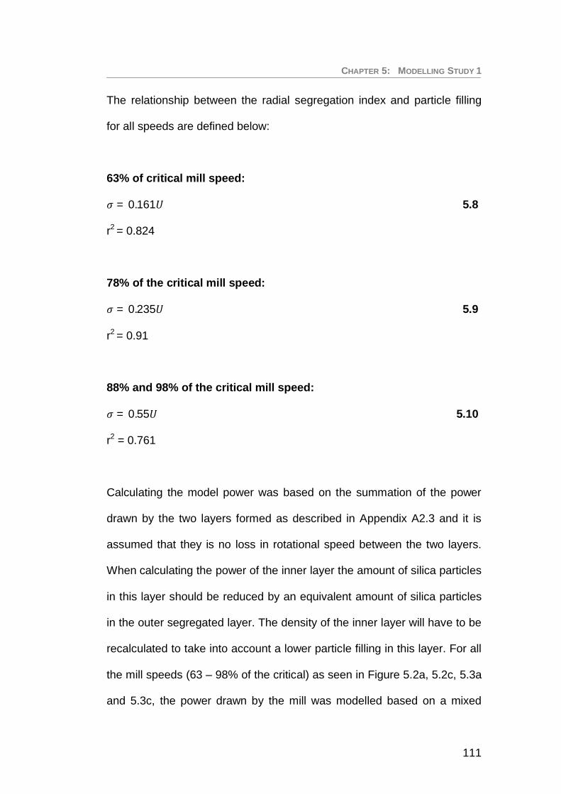
CHAPTER 5: MODELLING STUDY 1
111
The relationship between the radial segregation index and particle filling
for all speeds are defined below:
63% of critical mill speed:
= 0.161 5.8
r2 = 0.824
78% of the critical mill speed:
= 0.235 5.9
r2 = 0.91
88% and 98% of the critical mill speed:
= 0.55 5.10
r2 = 0.761
Calculating the model power was based on the summation of the power
drawn by the two layers formed as described in Appendix A2.3 and it is
assumed that they is no loss in rotational speed between the two layers.
When calculating the power of the inner layer the amount of silica particles
in this layer should be reduced by an equivalent amount of silica particles
in the outer segregated layer. The density of the inner layer will have to be
recalculated to take into account a lower particle filling in this layer. For all
the mill speeds (63 – 98% of the critical) as seen in Figure 5.2a, 5.2c, 5.3a
and 5.3c, the power drawn by the mill was modelled based on a mixed

CHAPTER 5: MODELLING STUDY 1
112
charge model and a segregated charge model. The solid line corresponds
to the mixed charge model while the broken line corresponds to the
segregated charge model. At the lower mill speeds of 63% and 78% of the
critical there is no difference between the powers calculated by either the
mixed or segregated charge models. This is most likely due to the outer
layer comprised of silica sand not being thick enough and of a lower
density as compared to the inner layer thus the power calculated for this
outer layer by the power model cannot cause a substantial difference in
power when the two charge models are considered. For higher mill speeds
of 88% and 98% of the critical there is an 8 and 11% difference
respectively between the powers calculated by the mixed and segregated
charge models.
Of importance to be learnt about radial segregation is that it can influence
the load behaviour substantially. In this case increased cataracting came
about partly due to the fact that the segregated silica sand encouraged
more lift in the outer layer of balls at high particle fillings as seen in Figure
5.2d and 5.3b and for high mill speeds such as 98% of the critical
centrifuging of the load resulted as seen in Figure 5.3d. Cataracting and
centrifuging are known to be accompanied by a loss in power drawn in
tumbling mills and for these experiments a shift in maximum power to a
lower particle filling. If a mill was to operate at this low particle filling
increased ball wear would result as most of the balls would be
concentrated to the middle of the charge with very little particles presents

CHAPTER 5: MODELLING STUDY 1
113
in the void spaces as seen in Figure 5.5b. The grinding kinetics will also be
affected as they will be less breakage resulting due to reduced chances of
ball-ore contact and most likely this would be accompanied by a loss in
product throughput. Operating the mill at speeds where more mixing of the
charge results is to be encouraged and possibly designing liners that
would throw the charge onto the free surface of the load as this would
encourage mixing.
5.2.3 MODELLING OF THE FINE PARTICLE EFFECTS
The inductive probe signal, load behaviour and power modelling for the
mill speeds of 63, 78% and 88% of the critical speed can be seen in Figure
5.8. For the fine particle case at the mill speeds of 63%, 78% and 88% of
the critical speed as in Figure 5.8a, 5.8c and 5.8e respectively, the toe and
shoulder angular positions do not vary with particle filling. The toe and
shoulder models were left as defined by Morrell (1993).
Essentially the form depicts that the toe and shoulder angular positions
only vary with mill speed and load filling which is similar to the fine particle
load behaviour case. In this case no radial segregation occurs in the load
as the extent in voltage drop for a balls only load (particle filling = 0%)
compared to a load with a particle filling of 150% are similar as indicated in
Figure 5.8b. Morrell’s mixed charge power model (Appendix A2.1) was
capable of modelling adequately the mill’s power draw up to a particle
filling of 100% for the mill speeds between 63% and 88% as in Figure

CHAPTER 5: MODELLING STUDY 1
114
5.8a, 5.8c and 5.8e. Beyond the particle filling of 100% the load expansion
and pool formation models were incorporated into Morrell’s model and
used to account for power loss in the mill. In the modelling of power for
particles greater than 100% it is assumed that the excess volume of
particles above the volume that correspond to a particle filling of 100% can
either go to expanding the load or forming a pool comprised of fine silica
particles only or it can be split between pool formation and load expansion
in some pre-defined ratio.
For load expansion the volume of the load increases thus this results in
the total load filling increasing and a corresponding drop in the density of
the load (Appendix A2.1). For ball mills operating under normal conditions
it is usual to take the total mill filling to be equal to the ball filling though in
the case where the mill was overfilled a total filling was considered which
included the fractional volume of the mill that the balls occupied plus the
excess volume of particles above a particle filling of 100%. Morrell’s power
model has a strong dependency on the mill filling and this is displayed by
the mill power modelled by for the load expansion model increasing with
particle filling (Figure 5.8a, 5.8c & 5.8e) despite a 16% drop in the load
density from the particle filling of 100% to 160%. Under an exclusive load
expansion model the mill’s power draw was overestimated.

CHAPTER 5: MODELLING STUDY 1
115
a) Load orientation and power model – FineParticles (Mill speed = 63%)
b) Inductive probe signal - Fine Particles(Mill speed = 63%)
c) Load orientation and power model – FineParticles (Mill speed = 78%)
d) Inductive probe signal - Fine Particles(Mill speed = 78%)
e) Load orientation and power model – FineParticles (Mill speed = 88%)
f) Inductive probe signal - Fine Particles(Mill speed = 88%)
Figure 5.8: Load orientation, power and the inductive probe average
signal for the mill speeds of 63%, 78% and 88% of the critical

CHAPTER 5: MODELLING STUDY 1
116
For the pool formation case a pool made up of silica particles only was
generated using numerical methods as described in Appendix A2.4. The
pool’s volume is calculated by gradually incrementing the pool’s height in
the Simpson’s method up to where the resulting pool volume is equal to
the volume of excess particles above the particle filling of 100%. The
location of the centre of gravity of the pool is then calculated from the
resulting pool shape together with its corresponding torque and power
draw. The pool’s power draw is then reduced from the net power draw
calculated by Morrell’s power model for the rest of the load. Here the load
is assumed to remain at a constant load volume of 20% and its density
remains constant for the particle fillings of 100 – 160%. Under the pool
formation model the mill’s power draw is under estimated. As the mill
speed is increased the experimental power tends to lean towards pool
formation rather than load expansion. This then led to considering
modelling a ratio split between load expansion and pool formation.
For the ratio split between load expansion and pool formation the
excess volume of particles above a particle filling of 100% is split in
increments of 10% between the volume of particles contributing to load
expansion and the volume of particles that contribute to pool formation. A
typical example would be 90% of the excess volume of particles going to
load expansion and 10% going to pool formation and the percentage
contribution is adjusted by 10% for the next power calculation (i.e. the
next step would be 80% load expansion and 20% pool formation). At 63%

CHAPTER 5: MODELLING STUDY 1
117
of the critical mill speed the experimental power at the particle filling of
150% lies between the ratio split of 40:60 and 30:70 (pool formation: load
expansion) as seen in Figure 5.8a, while for the mill speed of 88% the
experimental power lies between the ratio split of 60:40 and 50:50 (pool
formation: load expansion) as seen in Figure 5.8e. Increasing the mill
speed would most likely cause a larger pool to be formed. It can be seen
that taking the ratio split into account one can model the power drawn by
the mill more accurately than a model that is based on load expansion only
or pool formation only.
Figure 5.9 shows the inductive probe signal, load behaviour and power
modelling for the mill speed of 98% of the critical speed. Above the particle
filling of 40% the load centrifuged as indicated in Figure 5.9b by the
asterisk on the corresponding particle fillings. No toe and shoulder angular
positions were obtained for these particle fillings thus it was assumed that
for the purpose of power modelling the toe and shoulder angular positions
will be the same as that obtained from the particle filling of 40%. For the
particle fillings between 0 - 40%, Morrell’s mixed charge model (Appendix
A2.1) was used to calculate the power draw. The model estimates the
power well. In the power modelling for particle filling greater than 40% the
mill’s power draw was modelled using the mixed centrifuged charge model
described in Appendix A2.2 as no radial segregation of particles occurred.
It was assumed that either a 6mm ball layer centrifuged that corresponds
to the smallest ball size or an 8mm ball layer centrifuged that corresponds

CHAPTER 5: MODELLING STUDY 1
118
to an average ball size. The solid line in Figure 5.9 corresponds to the
6mm ball layer centrifuging while the broken line corresponds to the 8mm
ball layer centrifuging. Under the assumption of a 6mm ball layer
centrifuging the experimental power draw was modelled adequately while
under the assumption of an 8mm ball layer centrifuging the power draw
was under estimated.
a) Load orientation and power model –Fine Particles (Mill speed = 98%)
b) Inductive probe signal - Fine Particles(Mill speed = 98%)
Figure 5.9: Load orientation, power and the inductive probe average
signal for the mill speeds of 98% of the critical speeds
5.3 CONCLUSION
For coarse particle fillings it is important to modify Morrell’s toe and
shoulder models to account for their variations with particle fillings. The
structure of Morrell’s C model allows for the incorporation of radial
segregation and centrifuging of silica particles. The effects of radial
segregation on the power were studied through the comparison of a mixed

CHAPTER 5: MODELLING STUDY 1
119
charge power model and the segregated charge power model. No
difference between the estimated powers from the two models was seen
at low mill speeds (i.e. < 88% of the critical speed) but increasing the mill’s
speed a difference was noticed. No attempt was made in incorporating the
effects of cataracting into Morrell’s C model thus for load behaviours
where excessive cataracting occurred the model’s ability of modelling
adequately the mill’s power was substantially degraded. Centrifuging of
the load at high mill speeds and particle fillings was incorporated into
Morrell’s C model thus improving mill power estimation.
For fine particle fillings Morrell’s mixed charge model was capable of
modelling adequately the mill’s power draw up to particle fillings of 100%.
No modifications were made to the models of the toe and shoulder of the
load as proposed by Morrell. Beyond particle filling of 100%, two models
were compared to explain the loss in mill power at high particle fillings this
are the load expansion and the particle pool formation models. Neither of
the two models used independently could explain the power loss so a
compromise between load expansion and pool formation models made it
possible to model the power drawn by the mill at particle fillings beyond
100%.

CHAPTER 6
MODELLING STUDY 2Modelling of particle filling and size effects on the load behaviour and
power in a dry pilot mill: Torque Arm Model
Moys power model was used to model the power draw data from the
experimental study on the effects of particles on the power. This model
was chosen due to the fact that it was developed based on the semi
phenomenological understanding of the mill’s load behaviour and could
relate the non linear dependency that a mill’s power has on ball filling, mill
speed and particle filling. In the model it was assumed that the charge was
well mixed and that at particle fillings greater than 100% the load
expansion model was valid. The parameter N* was used to model the
effects particle filling has on the mill’s power draw. Through the
understanding of the load behaviour signals while modelling the power
better estimation of the mill’s power draw resulted.
6

CHAPTER 6: MODELLING STUDY 2
121
6.0 INTRODUCTION
The torque-arm model has been widely used to develop power models
that are empirical, simplistic and in many instances inadequate in properly
relating the dependency of the mill filling on mill speed to the power
especially at high mill fillings and mill speeds. Despite this Bond’s power
model has been used to size many mills and has worked relatively well
(Bond, 1961). In instances where a knowledgeable individual would like to
determine a mill’s power; the Bond power model becomes an attractive
option due to its simplicity. A more complex model does exist which is
based on Discrete Element Methods and it can penetrate the non linear
dependency that mill variables have on the mill power (Mishra & Rajamani,
1992; Cleary, 1998 and Potapov et al, 2007).
The aim of this chapter is to investigate the ability Moys power model has
in modelling the effect of increasing coarse or fine particle fillings have on
a mill’s power draw.
6.1 MOYS POWER MODEL FRAMEWORK
Moys (1993) developed a power model based Bond’s power model. With a
departure from Bond’s empirical outlook, Moys took on developing a
power model that was based on the semi-phenomenological
understanding of the load behaviour within a mill. Here the model structure
reflected the complex non linear dependence of mill power on mill filling

CHAPTER 6: MODELLING STUDY 2
122
and mill speed. Furthermore the effects of slurry viscosity and liner design
could be related to model parameters.
In this model two extremes of load behaviour are coupled together so as to
describe the mill power over a wide range of operating conditions. These
extremes of load behaviour are:
Cascading load: Dominant at low mill speeds and can be
adequately described by the torque-arm model.
Centrifuging load: Dominant at high speeds and responsible for the
loss in power in mills.
It should be noted that by coupling these two extremes of load behaviour
the model does not describe the energy recovered when cataracting
media strike the descending mill shell and impart some of their energy.
Thus in Moys model the non-centrifuged active portion of the load will
draw power according to Bonds power model applied to a mill with a
reduced effective diameter and the centrifuged portion of the load draws
no power.
Moys power model for the active portion of the load is:
sin 6.1

CHAPTER 6: MODELLING STUDY 2
123
A model that relates the thickness of the centrifuged layer to the mill’s
operating variables is:
6.2
Where N* and N are parameters that are used to quantify the effect of mill
speed on the load behaviour. N* is virtually independent of liner design. J
is a parameter that governs the strength of the dependency of on the
load filling J and will be a strong function of liner profile design.
The effective diameter of the mill (Deff) is given by:
= ( ) 6.3
Here it is assumed that the thickness of the centrifuged layer is .
The effective mill filling (Jeff) is given by:
=( )
( )< 0.5[ ( ) ]
0, 0.5[ ( ) ]6.4
A simplification of equation 6.4 was proposed by Moys. The simplification
is:
= 20, 2 6.5

CHAPTER 6: MODELLING STUDY 2
124
6.2 ANALYSIS AND DISCUSSIONS
In chapter 4 it was seen that an increase in the particle filling can lead to
an increase in cataracting and centrifuging of the load even at normal mill
operating conditions. Such examples can be seen in the load behaviour
signals for coarse particles at the mill speed of 78% of the critical speed
with particle fillings between 110 - 150% (Figure 4.5a) and likewise for the
mill speed of 88% of the critical speed with particle fillings between 80 -
150% (Figure 4.5b). In this study an attempt to model the effect of particle
filling on the mill power will be made using Moys power model through a
proposal of a relationship between the model parameter N* and particle
filling.
To establish the initial parameter set to be used in the regression analysis
for the particle filling effects on power; data from the ball only load
experiments at the mill speeds of 63, 78, 88 and 98% of the critical mill
speed were used. This was important so as to reduce the number of
parameters to be established while modelling the particle filling effects on
power thus leading to the parameters K, , J, and N in Moys power
model being held constant while searching for parameter N*. For the balls
only load the value of N* was kept at 136 similar to what Moys (1993)
suggested in his analysis. The angle of repose was kept at 45o.The model
parameters seen in Table 6.1 were established from the regression
analysis conducted on a load comprised of balls only. Further information

CHAPTER 6: MODELLING STUDY 2
125
of the regression analysis can be obtained in Appendix A4.1 and being
more specific Table A4.1 and Figure A4.1.
Table 6.1: Established initial parameters for a ball only load
Parameter ValueK 0.124
0.836J 2.935N 1.018
6.2.1 MODELLING OF COARSE PARTICLE EFFECTS ON POWER
For coarse particles at the mill speed of 63% of the critical as seen in
Figure 6.1a and tabulated in Table A4.2 of Appendix A3.1, Moys model
was capable of modelling adequately the experimental power well across
almost all values of particle fillings. The established value of parameter N*
across all particle fillings remained at 136 suggesting that at this mill speed
increasing particle filling even up to 150% has no effect on power draw.
For this mill speed at particle fillings less than 100%; it was anticipated that
particles will not have any substantial influence on the power as no
cataracting of balls onto the down coming shell occurred and likewise no
centrifuging was detected by the inductive probe as seen in Figure 6.1b.
Thus the only effect particles would have is increasing the mass of the
load. At particle fillings greater than 100% two possibilities occurs i.e.
expansion of the load or pooling of particles. In this modelling study the
load expansion theory was used in conjunction with Moys power model

CHAPTER 6: MODELLING STUDY 2
126
thus leading to a slight decrease in the model’s power and likewise a slight
under estimation of the experimental power draw for particle fillings greater
than 100%. In addition in Moys power model it is assumed that the charge
is well mixed which was not the case for particle filling greater than 100%
as segregation occurred as seen in Figure 6.1b. No attempt was made to
model the segregation.
a) Moys power model – Coarse Particles(Mill speed = 63%)
b) Inductive probe signal - Coarse Particles(Mill speed = 63%)
c) Moys power model – Coarse Particles(Mill speed = 78%)
d) Inductive probe signal - coarse particles(Mill speed = 78%)
Figure 6.1: Moys power model predictions and the inductive probe
average signal for the mill speeds of 63% and 78% of the
critical

CHAPTER 6: MODELLING STUDY 2
127
At the mill speed of 78% of the critical as seen in Figure 6.1c; the power
model was capable of modelling adequately the experimental power over
the full range of particle fillings. For the particle filling where substantial
cataracting occurred in conjunction with a significant loss in power drawn
by the mill the value on N* in the model decreased to 78.32 as seen in
Table A4.3 in Appendix A4.1. It should be noted here that this substantial
decrease in power was a result of balls cataracting on the descending mill
shell and occurred only at the particle filling of 150%. Thus despite
substantial cataracting occurring at a filling of 110% as seen in Figure
6.1d; Moys model does not activate the model that determines the
centrifuged layer thickness as no substantial power loss is observed in the
experimental data.
At the mill speeds of 88 and 98% of the critical, two different methods were
used to describe the relationship between parameter N* and the particle
filling. Initially parameter N* was made independent of particle filling in an
attempt to use as few parameters as possible. In this case the power
model estimations indicated by N* = 88 seen in Figure 6.2a and N* = 98
seen in Figure 6.2c show a significant deterioration in the model’s ability to
model the power draw beyond the particle filling of 70%. At particle fillings
greater than 70% for the mill speed of 88% and likewise beyond the
particle filling of 60% for the mill speed of 98% of the critical the load
behaviour is dominated by significant cataracting of the load followed by
centrifuging of the load at high particle fillings. Due to the influence

CHAPTER 6: MODELLING STUDY 2
128
particles have on the load behaviour at particle fillings greater than 70% at
the mill speeds of 88 and 98% of the critical it was deemed reasonable to
use a linear model to relate the parameter N* to the particle filling. For
Moys power model predictions with a linear model defined by N* = cU + d
seen in Figure 6.2a and Figure 6.2c also displayed a significant
deterioration in the model’s ability to describe the power draw at particle
filling greater than 70%.
a) Moys power model – Coarse Particles(Mill speed = 88%)
b) Inductive probe signal - Coarse Particles(Mill speed = 88%)
c) Moys power model – Coarse Particles(Mill speed = 98%)
d) Inductive probe signal - Coarse particles(Mill speed = 98%)
Figure 6.2: Moys power model predictions and the inductive probe
average signal for the mill speeds of 88% and 98% of the
critical

CHAPTER 6: MODELLING STUDY 2
129
By using a single constant value to define parameter N* (i.e. N* = 88 and
N* = 98 as in Figure 6.2) or a linear model (i.e. N*= cU + d as in Figure
6.2) over conditions where both cataracting and centrifuging occur as a
result of increasing particle filling reduced the model’s ability to describe
the power drawn by the mill. In the case of cataracting conditions it can be
clearly seen from the experimental data in Figure 6.2 that increasing
particle filling led to an increase in cataracting of the load coupled with a
reduction in the mill’s power draw. While in the case of centrifuging
increasing particle filling while maintaining a constant mill speed led to an
increase in the mills power draw. For the mill speed of 88% of the critical
the load centrifuged at a particle filling of 150%, as seen in Figure 6.2a,
and was associated with an 11% increase in the experimental power draw.
Likewise for the mill speed of 98% of the critical speed, the centrifuging of
the load that occurred after the particle filling of 100% as seen in Figure
6.2c was associated with a 5% increase in power draw. Possibly under the
circumstances where increasing particle filling causes a change in the load
behaviour the model that defines parameter N* should be limited to cover
only a specific load condition.
Through the understanding of the load behaviour and the influence particle
filling has on it for the mill speed of 88 and 98% of the critical it was best to
use separate linear models to define the relationship between parameter
N* and the particle filling when the load is cataracting and when it is
centrifuging. For the linear power model predictions indicated by N*=aU+b

CHAPTER 6: MODELLING STUDY 2
130
as seen in Figure 6.2a and Figure 6.2c, it can be seen that by using two
separate linear models to relate parameter N* to the particle filling
considerably improves the models ability to describe the power draw. The
regression analysis data for the mill speeds of 88% of the critical can be
seen in Table A3.4 through to Table A3.6 in Appendix A3.2. Likewise for
the mill speed of 98% of the critical the regression analysis data can be
seen in Table A3.7 through to Table A3.9 in Appendix A3.2.
6.2.2 MODELLING OF THE FINE PARTICLE EFFECTS ON POWER
For the fine particles at the mill speeds of 63%, 78% and 88% of the
critical speed no cataracting or centrifuging was experienced across any
particle fillings. This is seen in the inductive probe signals in Figure 6.3b,
6.3d and 6.3f. The fine particles possibly lubricate the load more efficiently
than coarse particles thus limiting the extent in which the load could
possibly cataract. This kind of load behaviour across these mill speeds
also led to a power draw that is relatively constant across all particle
fillings.
From the load behaviour investigation for the mill speeds between 63-88%
of the critical, it is possible to safely assume that increasing fine particle
filling has very little or no influence on the load behaviour and thus the
parameter N* could be independent of the particle filling. For particle
fillings greater than 100% the parameter N* in Moys power model was set
at the value of 64 for the mill speed of 63% of the critical (Figure 6.3a), a

CHAPTER 6: MODELLING STUDY 2
131
value of 78.98 for the mill speed of 78% of the critical (Figure 6.3c) and a
value of 89.2 for the mill speed of 88% of the critical (Figure 6.3e). Using
these values of the N* parameter for mill speeds between 63-88% of the
critical, Moys power model was capable of modelling adequately the
experimental power draw over most particle fillings. For the particle filling
of 150%, Moys power model over estimated the experimental power draw
by about 6%. It is possible that when excessive amounts of fine particles
are present in the mill (i.e. U > 100%) a powder pool possibly exists that
would cause a decrease in the power draw. In this modelling exercise the
load expansion theory was used in conjunction with Moys power model.
No investigations were conducted to look at the effects of a particle pool
on the power draw as this was dealt in quite some detail in section 5.2.3 in
Chapter 5. This once again strongly supports the possibility of a powder
pool being formed.
Using a linear model to define the dependency of parameter N* on the
particle filling (N* = aU + b) further improved the ability of Moys power
model in modelling adequately the experimental power draw for particle
fillings greater than 100% at the mill speed of 63% (Figure 6.3a), 78%
(Figure 6.3c) and 88% of the critical speed (Figure 6.3a). Although in the
case where the linear model is used the power loss is strongly related to
the centrifuged layer in Moys power model being thicker thus accounting
for the power loss.

CHAPTER 6: MODELLING STUDY 2
132
a) Moys power model – Fine Particles(Mill speed = 63%)
b) Inductive probe signal - Fine Particles(Mill speed = 63%)
c) Moys power model – Fine Particles(Mill speed = 78%)
d) Inductive probe signal - Fine Particles(Mill speed = 78%)
e) Moys power model – Fine Particles(Mill speed = 88%)
f) Inductive probe signal - Fine Particles(Mill speed = 88%)
Figure 6.3: Moys power model predictions and the inductive probe
average signal for the mill speeds of 63%, 78% and 88% of
the critical

CHAPTER 6: MODELLING STUDY 2
133
Interestingly; for the case of 98% of the critical speed as seen in Figure
6.4b the load behaviour was either in and active charge state or
centrifuged depending on the particle filling. This becomes interesting as
these are the two extremes in load behaviour that Moys power model is
based on i.e. either the load is comprised of an active cascading charge or
the combinations of an active charge and centrifuged charge. However it
should be made clear that in the centrifuged state (U > 60%) the behaviour
of the active load is not known and the load could either be cascading or
experiencing a significant amount of cataracting.
a) Moys power model – Fine Particles(Mill speed = 98%)
b) Inductive probe signal - Fine Particles(Mill speed = 98%)
Figure 6.4: Moys power model predictions and the inductive probe
average signal for the mill speeds of 98% of the critical
speeds
From Figure 6.4a it can be seen that Moys power model was capable of
modelling adequately the power over all particle fillings. For the mill speed
of 98% of the critical and for particle fillings greater than 40% the two

CHAPTER 6: MODELLING STUDY 2
134
methods that define the relationship between parameter N* and particle
filling were used in Moys power model. The use of the two models i.e. N* =
98.27 and N* = aU+b in Moys power model yield identical predictions of
the experimental power over all particle fillings greater than 40%. The
identical predictions are most likely due to the load conditions being similar
to the basis of Moys power model. Furthermore it should be noted that
after centrifuging occurred the power did increase and peak as the particle
filling increased. This is due to the fact that when a mill with a smaller
effective diameter is formed as a result of part of the active charge being
centrifuged it would behave as a new mill and its power should increase
with increasing particle filling provided that the mill speed is held constant.
The regression analysis data for the mill speeds of 63%, 78%, 88% and
98% of the critical can be seen in Table A3.10 through to Table A34.17 in
Appendix A3.3.
6.3 CONCLUSION
In this modelling study a torque arm model in the form of Moys power
model was used to model the mill’s power draw from the experimental
study conducted in Chapter 4. The experimental study offered a unique
data set whereby the mill’s power draw was obtained in conjunction with
load behaviour data from an inductive proximity probe at the mill speeds of
63%, 78%, 88% and 98% of the critical speed. Various conditions of load

CHAPTER 6: MODELLING STUDY 2
135
behaviour were encountered with increasing coarse and fine particle filling
such as segregation, cascading, cataracting, centrifuging and possibly the
pooling of particles. In the modelling it was assumed the charge was well
mixed and no attempts were made in modelling the impact cataracting of
the load has on the power. From the Moys power model the parameter N*
was chosen to model the effects of increasing particle filling has on the
mill’s power draw. Two model definitions were used in the study whereby
one kept the value of parameter N* to be constant and independent of
particle filling and the other made parameter N* vary linearly with particle
filling.
In the case of coarse particle filling at low mill speeds (i.e. 63% of the
critical) the power draw can be predicted using N* = 136 as previously
suggested by Moys (1993). It seems at such low speeds increasing the
coarse particle filling does not have any significant influence on the load
behaviour and likewise power draw. Increasing the mill speed to 78%,
88% and 98% of the critical a new value of parameter N* had to be
established particularly when the conditions of cataracting or centrifuging
prevail. For these mill speeds a better estimations of the mill’s power draw
resulted when the power draw at the conditions of cataracting and
centrifuged are modelled based on separate N* linear models as particle
filling is increased. This resulted from the fact that when balls cataract and
strike on the descending mill shell it is normally accompanied by a loss in
power draw for that mill speed. Increasing coarse particle filling increases

CHAPTER 6: MODELLING STUDY 2
136
the intensity of cataracting at that mill speed. When centrifuging occurs at
a constant speed while increasing the coarse particle filling it is
accompanied by an increase in the power drawn by the mill.
For the case of increasing fine particle filling at the mill speeds of 63, 78
and 88% of the critical a linear model would be the best to use in defining
the relationship between N* and the particle filling. At these mill speeds
there is a possibility that the loss in power occurs as a result of the
presence of a particle pool as no cataracting or centrifuging occurred.
Increasing the mill speed to 98% of the critical the relationship between
parameter N* and the particle filling could either be a constant value or a
linear model. By understanding the load behaviour improvements in the
modelling of a mill’s power draw can be brought about.

CHAPTER7
CONCLUSION AND
RECOMMENDATIONS
7

CHAPTER 7: CONCLUSION AND RECOMMENDATIONS
138
7.0 CONCLUSION
Many factors that influence the ball load behaviour have been previously
studied. It is known that a load comprised of balls only behaves quite
differently when ore is introduced into the mill. Different ore types and
sizes influence the ball load to varying extents. Typically in industry, while
refilling a ground out mill the operator would fill the running mill with ore up
to the point where the maximum power drawn by the mill is achieved. This
practice is from the fact that the mill power has a parabolic dependency on
the mill filling. Under filling the mill would result in an inefficient operation
of the mill due to ball and liner wear. Overfilling the mill would also result in
an inefficient mill operation due to a slowdown in grinding rates as a result
of the presence of excess particles in the mill. At the maximum power
draw it is generally assumed the load is well mixed and that the void
spaces between the balls are full with particles. To the operator this
translates to an efficient mill and maintains the maximum power draw as a
set point. This study sets to understand how particle filling and size
influence the ball load behaviour and power in a dry mill. The study mimics
the filling of an industrial ball mill from when it is empty to when it is 50%
overfilled with particles.
A novel technique in load behaviour measurements was used to conduct
this study. The technique made use of an inductive proximity probe to
measure the steel ball load position independently of the presence of
CHAPTER 7: CONCLUSION AND RECOMMENDATIONS
139
particles in the mill. Static and dynamic response test were performed on
the inductive probe to assess its suitability for load behaviour
measurements. The static test show that the inductive probe’s signal
varies linearly with an increase in distance from its sensing face of a
metallic target. The dynamic tests show that the probe takes 6.9ms to
reach 98% of its maximum signal value thus translating to an error of 2.54o
at the highest mill speed of 60.78rpm for the pilot mill used in this study. In
the case of industrial mills that typically run at lower mill speeds this error
would be insignificant. The probe was also tested in a mill as a means of
measuring the dynamic load behaviour. Load conditions such as
cataracting, centrifuging, ball packing, toe and shoulder positions as a
function of mill filling and speed were easily detected and distinguishable
in the probe’s signal. The probe exhibits superior shoulder angular position
measurement capabilities when compared to a force probe but the toe’s
angular position can be influenced with balls cataracting in this region.
Furthermore, the probe does not require complicated circuitry or signal
analysis algorithms. The inductive probe can be used in industrial mills
provided the necessary protection is made for the probe to operate in the
harsh conditions prevalent in the mill. For an industrial mill, it would be
preferred to use the probe for investigative studies rather than a
measurement device to obtain an additional control variable for the load
behaviour. Here the load behaviour could be easily measured as mill
operating variables are changed and a clear picture drawn as to how the
load responds. The information from such investigations could be used in

CHAPTER 7: CONCLUSION AND RECOMMENDATIONS
140
conjunction with the Discrete Element Model (DEM) simulators to further
understand the load behaviour in the mill. Possibly this would lead to
enhancing the design of the mill internals or select suitable operating
conditions that would lead to an optimal load behaviour prevailing. Caution
should be taken in selecting a sensor with a suitable measuring range due
to the fact that for the larger steel balls the signal will be noisier than the
probe response signals displayed in this thesis. Possibly, for mills
containing large ball sizes a different signal analysis technique could be
used based on a moving standard deviation of the signal response rather
than analysing the average signal response.
Increasing the particle filling of coarse silica sand particles at different mill
speeds between 63-98% of the critical mill speed led to excessive
cataracting of the load, radial segregation and centrifuging. These
changes in load behaviour as particle filling was increased at a set mill
speed led to variations in the experimental mill power draw trends. The
radial segregation of silica sand particles to the periphery of the load was
quantified and reveals that its intensity increases with an increase in mill
speed and particle filling. The depletion of the coarse particles from the
core of the load due to radial segregation causes an increased chance of
ball to ball contacts thus possibly leading to an increased ball wear rate.
The segregated silica sand causes excessive cataracting of the load onto
the exposed mill shell thus leading to a loss in the mill’s power. The
centrifuging of the segregated silica sand leads to further losses in mill

CHAPTER 7: CONCLUSION AND RECOMMENDATIONS
141
power. The maximum mill power drawn by the mill exhibits the tendency to
move to lower particle fillings as mill speed is increased. The steel balls
being located at the core of the load reduced their chances to damage or
break the silica particles thus possibly leading to the slowdown of grinding
rates within the mill. Mill power loss due to cataracting and centrifuging
further reduces the energy available for breakage of particles thus again
negatively impacting the grinding rates. Should radial segregation occur in
an industrial mill then the action of the operator chasing the maximum
power by increasing the mill’s particle filling would lead to the mill
operating inefficiently especially at high mill speeds (i.e. greater than 88%
of the critical speed). The development of the inductive probe to be used
as an additional online measurement for the early detection of segregation
would help the mill operator substantially.
The load comprised of fine silica particles behaved as one would expect
for mill speeds up to 88% of the critical. The load was only sensitive to
increases in mill speed thus leading to a rise in the shoulders angular
position. No sensitivity was established with particle filling increase at a
particular mill speed. The peak in mill power occurred at particle fillings
between 80 – 110% followed by a slight loss in mill power. At this stage it
was assumed that this loss in power is probably due to either load
expansion or a particle pool being formed at the toe of the load. None of
the two assumptions were validated experimentally. Unfortunately the
inductive probe can only sense the presence of metallic objects; thus it

CHAPTER 7: CONCLUSION AND RECOMMENDATIONS
142
would be important in such cases that a second probe would be needed
that can sense both metallic and non-metallic objects. Possibly a force
probe or a capacitive proximity sensor could be used to detect the powder
pool located at the toe of the load. Interestingly, the capacitive sensor can
be very effective in measuring the presence of non- metallic objects, the
density, thickness and location. The capacitive probe works by sensing
changes in the dielectric of the material and therefore changes in
capacitance due to the presence of a non-conductor in the sensing range.
The sensitivity of the sensor to the non-conductive target is directly
proportional to the dielectric constant of the material. When the mill speed
was increased to 98% of the critical the fine silica particle caused the balls
to centrifuge at a particle filling greater than 40% with a corresponding
peak in the mill’s power draw between particle fillings of 20 – 40%.
It should be noted that for both the coarse and fine particle experiments
the effect of the continuous removal of fine particles generated in the mill
by an air draft was not studied. Such an experiment would give an exact
replication of an industrial air swept mill. This continuous removal of the
right size particles can possibly change the load behaviour in the mill and
likewise its power draw. Furthermore, no work was conducted into the
effects that the various load behaviour conditions encountered have on the
grinding rates in the mill. This work would form a basis to establish the
effects that the various load behaviour conditions encountered in the
experiments have on the energy efficiency of grinding. From the

CHAPTER 7: CONCLUSION AND RECOMMENDATIONS
143
experimental study it can be seen that using the power alone to be the
sole indicator for finding a mill’s best operating point is not always the best
thing to do. Various conditions can arise within the mill that would lead to a
peak in power at low particle fillings thus increasing ball and liner wear
rates and leading to inefficient mill operations. With the greater use of
variable speed mills in the mining industry it becomes even more important
to understand how a mill would behave when various particle sizes are
being filled into the mill in relation to the mill speed. It would be highly
discouraged to operate a mill at speeds higher than 88% of the critical as
in both cases of coarse and fine particle fillings the load behaviour
changed dramatically and the conditions would lead to the mill being
operated inefficiently.
A modelling study was conducted using Morrell’s C model. The model was
chosen due to the fact that it contains physical descriptors of the load such
as the toe, shoulder and charge inner surface. Modifications to Morrell’s
model were made in the toe and shoulder models. A segregated charge
model was proposed for situations where radial segregation occurred. A
subtle difference was noted when the radial segregation power model
results were compared to that of the mixed charge model. A centrifuged
charge model was proposed which generally improved the model’s
capability of modelling the power draw during the centrifuging condition. In
the case of fine particles at high particle fillings (U>100%) a split between
a particle pool and load expansion model was proposed which improved

CHAPTER 7: CONCLUSION AND RECOMMENDATIONS
144
Morrell’s C model ability of modelling the fine particle power draw. The
modified Morrell C model was suitable in modelling the experimental
power draw apart from conditions where there was intense cataracting of
the load. No attempt was made to include the effects of the cataracting
portion of the load into Morrell’s model.
In a second modelling exercise the torque arm model in the form of the
Moys power model was used to model the experimental power draw. This
model was chosen due to the fact that it was developed based on the semi
phenomenological understanding of the mill’s load behaviour and could
relate the non linear dependency that a mill’s power has on ball filling, mill
speed and particle filling. The parameter N* was assumed to either vary
linearly with particle filling or be independent of particle filling. Improved
modellling come about when N* is related linearly to the particle filling.
With these modifications added to the N* model the modified Moys model
was capable of modelling the mill’s power draw sufficiently.
This modelling exercise demonstrated the importance of understanding
the impact that mill operating variables and mill design have on the load
behaviour and power draw and through this establish improvements that
can be made to existing power models so as to enhance the models ability
in modelling adequately a mill’s power draw. Both the Morrell’s C power
model and Moys power model with the necessary modifications were

CHAPTER 7: CONCLUSION AND RECOMMENDATIONS
145
capable of modelling adequately the power drawn by the mill for most of
the conditions occurring in the mill.
The Discrete Element Model (DEM) treats the charge as discrete particles
which make it quite a powerful tool in simulating the complex load
behaviours experienced in this study and likewise its corresponding power
draw. Currently most of the available DEM packages can model particles
with different densities and likewise shapes which will be quite useful in
modelling the experiments conducted. Furthermore should a researcher
wish to simplify the problem by using spherical particles for both the balls
and silica particles with no breakage of particles occurring then the
differences in the load behaviours can be established and necessary
adjusting of the DEM model parameters can be done wisely and in an
informed manner.
Some DEM simulators couple their models with Discrete Grain Breakage
(DGB) models, Computational Fluid Dynamic (CFD) models, Smooth
Particle Hydrodynamic (SPH) models and Multi-Phase Flow models
(Cleary, 2001; Potapov et al, 2007). In most cases there has been a lack
of DEM validation data to test their simulators against the reality over a
wide range of conditions from a controlled experiment. The coarse and
fine particle results can be used to validate DEM simulations and in
particular when the researcher’s interests involve a charge mixed with
particles of different densities and of various particle sizes and shapes
CHAPTER 7: CONCLUSION AND RECOMMENDATIONS
146
undergoing breakage. When breakage of particles are involved in a DEM
simulator the problem becomes handling the great number of particles
resulting from the breakage events (i.e. tracking and storing information
related to the new particles) as this would require tremendous computing
power and memory and it would take a long period of time to obtain
sensible results.
For the coarse particle case, the use of the technique published by
Potapov et al (2007) of coupling the DEM with the PBM model to form
what they refer to as the Fast-Breakage model would simplify the DEM
simulation and bring down considerably the simulation time. For the fine
particle case, a tremendous amount of particles will be involved from the
start of the simulation and will continue to increase as breakage occurs in
the mill. Possibly treating the fine particles as slurry would further simplify
the problem. Fine particles have the ability of easily pouring through the
void spaces in the charge without significantly affecting the behaviour of
the ball load. It is important to establish the bottom size limit of the size
distribution where below this size the particles would be regarded as
slurry.

REFERENCES

REFERENCES
148
Agrawala, S., Rajamani, R. K., Songfack, P. and Mishra, B. K., 1997.
Mechanics of media motion in tumbling mills with 3D Discrete
Element Method. Minerals Engineering, Volume 10(2), pp. 215 -
227.
Austin, L. G., Klimpel, R. R. and Luckie, P. T., 1984. Process engineering
of size reduction: Ball Milling. Society of mining engineers of the
American Institute of Mining, Metallurgical and Petroleum
Engineers, Inc.
Behera, B., Mishra, B. K. and Murty, C.V.R., 2007. Experimental analysis
of charge dynamics in tumbling mills by vibration signature
technique. Minerals Engineering, Volume 20(1), pp. 84 – 91.
Bond, F.C, 1961a. Crushing and grinding calculations Part 1. British
Chemical Engineering, Volume 6(8), pp. 378 – 385.
Bond, F.C, 1961b. Crushing and grinding calculations Part 2. British
Chemical Engineering, Volume 6(8), pp. 543 –548.
Cundall, P.A. and Strack, O. D. L, 1979. Discrete numerical model for
granular assemblies. Geotechnique, Volume 29(1), pp. 47 –64.
Campbell, J., Spencer, S., Sutherland, D., Rowlands, T., Weller, K.,
Cleary, P. and Hinde, A., 2001. SAG mill monitoring using surface
vibrations. Proceedings of the International Autogenous and Semi-
Autogenous grinding technology conference 2, pp. 373-385.
Campbell, J. J., Holmes, R. J., Spencer, S. J., Sharp, V., Davey, K. J.,
Barker, D. G. and Phillips, P. L., 2003. The collection and analysis
of single sensor surface vibration data to estimate operating

REFERENCES
149
conditions in pilot scale and production scale AG/SAG mills.
Proceedings: XXII International Mineral Processing Congress, pp.
280 – 288.
Cleary, P. W., 1998. Predicting charge motion, power draw, segregation
and wear in ball mills using discrete element methods. Minerals
Engineering 11(11), pp. 1061-1080.
Cleary, P. W., 2001. Recent advances in DEM modelling of tumbling mills.
Minerals Engineering 14(10), pp. 1295-1319.
Davis, E. W., 1919. Fine crushing in ball mills. Transactions of the
American Institute of Mechanical Engineers (AIME). Volume 61, pp.
250.
Dong, H. and Moys, M. H., 2003. Load behaviour and Mill power.
International Journal of Minerals Processing, Volume 69. pp 11-28.
Dong, H., Couvas, C., Breetzke, M. and Moys, M., 2005. Measurement of
load behaviour of an Eskom coal mill. SAIMM-Mineral Processing
Conference, Cape Town, OR20, pp. 38.
Dupont, J. F. & Vien, A., 2001a. Continuous SAG volumetric charge
measurements. Proceedings of the 33rd Annual Canadian Mineral
Processing AGM, CIM, Ottawa, Canada. pp. 51 – 67.
Dupont, J. F. & Vien, A., 2001b. Direct measurement and control of SAG
volumetric loads using embedded sensors. Preprints of the SME
annual meeting, USA. pp. 1 – 5.
Fuerstenau, D. W., Kapur, P. C. and Velamakanni, 1990. A multi-torque
model for the effects of dispersants and slurry viscosity on ball

REFERENCES
150
milling. International Journal of Minerals Processing, Volume 28, pp
81-98.
Gugel, K., Palacios, G., Ramirez, J. and Parra, M., 2003. Improving ball
mill control with modern tools based on digital signal processing
(DSP) technology. Cement industry technical conference. pp. 311 –
318.
Govender, I., Powell, M. S. and Nurick, G. N., 2002. Automated imaging
technique to track the 3D motion of particles. Experimental
Mechanics. Volume 42 (2), pp 153 - 160.
Govender, I., McBride, A. T., and Powell, M. S., 2004. Improved
experimental tracking techniques for validating discrete element
methods simulations of tumbling mills. Experimental Mechanics.
Volume 44 (6), pp 593 - 607.
Harding, H., 1939. The ‘electric ear’, a device for automatically controlling
mills by their sound. Transactions of the American Institute of
Mining, Metallurgical and Petroleum Engineers. Volume 134, pp
371 - 380.
Jain, N., Ottino, J. and Lueptow, R., 2005. Regimes of segregation and
mixing in combined size and density granular systems: an
experimental study. Granular Matter 7, pp. 69 – 81
Jaspan, R. K., Young, G. J. C and Mellor, M. S., 1986. ROM mill power
draft control using multiple microphones to determine mill load.
Gold 100: Proceedings of the international conference on gold.
SAIMM, Volume 2, pp 483-492.

REFERENCES
151
Kalala, J. T., Breetzke, M. and Moys, M., 2007. Study of the influence of
liner wear on the load behaviour of an industrial tumbling mill using
Discrete Element Methods (DEM). International Journal of Mineral
Processing. Volume 86(1-4), pp 33-39.
Kiangi, K. and Moys, M. H., 2006. Measurement of load behaviour in a dry
pilot mill using an inductive proximity probe. Minerals engineering
Volume 19(13), pp. 1348-1356.
Kolacz, J., 1997. Measurement system of the mill charge in grinding ball
mill circuits. Minerals Engineering, Volume 10, No. 12, pp 1329-
1338.
McIvor, R. E., 1983. Effect of speed and liner configuration on ball mill
performance. Mining Engineering, Volume 35(6), pp 617 – 624.
Mishra, B. K., and Rajamani, R. J., 1992. The discrete element method for
the simulation of ball mills. Applied Mathematical Modelling, Volume
16, 598-604.
Morrell, S., 1993. The prediction of power draw in wet tumbling mills. PhD
Thesis. University of Queensland.
Moys, M. H., 1985. The measurements of parameters describing the
dynamic behaviour of the load in a grinding mill. Journal of the
South African Institute of Mining and Metallurgy, Volume 85(2), pp
51-63.
Moys, M. H., 1993. A model of mill power as affected by mill speed, load
volume and liner design. Journal of the South African Institute of
Mining and Metallurgy, Volume 93(6), pp 135-141.

REFERENCES
152
Moys, M. H., Van Nierop, M. A. and Smit, I., 1996. Progress in measuring
and modelling load behaviour in pilot and industrial mills. Minerals
Engineering, Volume 9(12), pp 1201-1214.
Moys, M. H., Smit, I. and Stange, W., 1996. The measurement of forces
exerted by the load on liners in rotary mills (wet and dry).
International Journal of Minerals Processing, Volume 44-45, pp
383-393.
Nesbit, P. Q. and Moys, M. H., 1998. Load behaviour in the HICOM
nutating mill. Minerals Engineering, Volume 11(10), pp 979 - 988.
Pax, R., 2001. Non-Contact acoustic measurement of in-mill variables of
SAG mills. Proceedings of the International Autogenous and Semi-
Autogenous grinding technology conference 2, pp. 386-393.
Potapov, A., Herbst, J., Song, M. and Pate, W., 2007. A DEM-PBM fast
breakage model for simulation of comminution processes.
Proceedings of Discrete Element Methods, Australia.
Powell, M. S. 1991. The effect of liner design on the motion of the outer
grinding elements in a rotary mill. International Journal of Minerals
Processing, Volume 31(3-4), pp 163-193.
Powell, M. S. and Nurick, G. N., 1996a. A study of charge motion in rotary
mills Part 2- Experimental work. Minerals Engineering, Volume 9,
No. 3, pp 343 – 350
Powell, M. S. and Nurick, G. N, 1996b. A study of charge motion in rotary
mills Part 3 – Analysis of results. Minerals Engineering 9(4), pp.
399-418.

REFERENCES
153
Qiu, X., Potapov, A., Song, M. and Nordell, L., 2001. Prediction of wear of
mill lifters using DEM. Proceedings of the international Autogenous
and Semi-Autogenous Grinding Technology, Vancouver, Canada.
Volume IV, pp. 260-265.
Rose, H. E. and Sullivan, R. M. E, 1958. Treatise on the internal
mechanics of ball tube and rod mills. Constable and Company Ltd.,
London.
Smit, I., 2000. The effect of slurry viscosity and mill speed on the
behaviour of a rotary grinding mill. MSc Dissertation. University of
the Witwatersrand, Johannesburg.
Skorupa, J. and Moys, M. H., 1993. Measurement of the radial and
tangential forces exerted by the load on a liner in a ball mill as a
function of load volume and mill speed. International Journal of
Minerals Processing, Volume 37, pp 239 – 256.
Tangsathitkulchai, C., 2003. Effects of slurry concentration and powder
filling on the net mill power of a laboratory ball mill. Powder
Technology 137(3), pp. 131-138.
Tano, K; Palsson, B and Sellgren, A, 2005. Online lifter deflection
measurements showing flow resistance effects in grinding mills.
Minerals Engineering 18(11), pp. 1077-1085.
Van Nierop, M. A., and Moys, M. H., 2001. Exploration of mill power
modelled as a function of load behaviour. Minerals Engineering,
Volume 14(10), pp 1267-1276.

REFERENCES
154
Vermeulen, L. A., Ohlson, M. J. and Schakowski, F., 1984. Continuous
monitoring of information from the inside of a rotary mill. Journal of
the South African Institute of Mining and Metallurgy, Volume 85(2),
pp 51-63.
Vermeulen, L. A. and Howat, D. D., 1986. Fluctuations in slip of the
grinding charge in rotary mills with smooth liners. International
journal of mineral processing, Volume 16, pp. 153 – 168.
Watson, J. L, 1985. An analysis of grinding media noise. Powder
Technology, Volume 41, pp 83-89.
White, H. A, 1905. Theory of the tube mill. Journal of the Chemical,
Metallurgical and Mining Society of South Africa, Volume 5, pp 290-
305.
Zeng, Y. and Forssberg, E., 1991. Effect of powder filling fraction on
particle size and energy consumption in coarse grinding.
Scandinavian Journal of Metallurgy 20, pp. 300 – 304.
Zeng, Y. and Forssberg, E., 1992. Effects of operating parameters on
vibration signal under laboratory scale ball grinding conditions.
International journal of mineral processing, Volume 35, pp 273 –
290.
Zeng, Y. and Forssberg, E., 1993. Monitoring grinding parameters by
signal measurements for an industrial ball mill. International journal
of mineral processing, Volume 40, pp 1 – 16.

APPENDIX 1
EXPERIMENTALRESULTS
A1

APPENDIX 1: EXPERIMENTAL RESULTS
A1.1 EXPERIMENTAL DATA FOR THE COARSE PARTICLE EXPERIMENTS
Mill speed of 63% of the critical:
Mill speed of 78% of the critical:
Particle Filling Average Standard deviation Average Standard deviation Average Standard deviation Average Standard deviation Average Standard deviation% % % Degrees Degrees Degrees Degrees Nm Nm watts watts
0 62.99 0.09 153.25 1.81 290.93 2.66 43.33 0.20 167.94 0.9220 62.43 0.40 155.01 2.48 285.25 1.10 45.20 0.28 173.93 1.8540 63.22 0.37 156.94 3.08 290.43 2.45 47.38 0.19 184.66 1.1060 62.58 0.31 156.49 2.65 291.19 1.95 48.69 0.27 187.75 1.6070 63.00 0.45 158.64 5.43 292.66 1.90 49.37 0.15 191.79 1.2780 64.45 0.43 159.75 6.63 294.56 1.83 50.59 0.19 201.00 1.5790 63.68 0.45 166.70 8.00 295.22 1.72 51.02 0.30 200.29 1.47
100 64.11 0.27 155.50 4.32 296.27 1.16 51.57 0.30 203.69 1.59110 64.02 0.42 154.63 1.54 297.72 1.00 52.98 0.22 209.05 1.55150 64.20 0.26 156.11 5.67 303.84 2.43 54.00 0.44 213.53 2.33
Speed Toe Shoulder Torque Power
Particle Filling Average Standard deviation Average Standard deviation Average Standard deviation Average Standard deviation Average Standard deviation% % % Degrees Degrees Degrees Degrees Nm Nm watts watts
0 75.32 0.12 168.45 23.45 300.41 3.67 44.90 0.31 207.92 1.3220 76.59 0.11 163.16 4.82 291.52 2.69 47.52 0.23 224.04 1.2340 77.10 0.13 163.39 6.73 297.31 3.12 48.85 0.37 231.81 1.9060 77.11 0.15 167.51 7.17 297.64 2.20 50.06 0.18 237.49 1.1670 76.67 0.11 172.68 6.98 299.08 1.78 50.55 0.18 238.44 0.9080 78.31 0.12 175.37 4.60 302.64 2.34 52.29 0.21 252.00 1.1290 78.46 0.09 173.58 5.85 305.59 3.79 52.14 0.23 251.65 1.07
100 78.11 0.10 161.68 2.70 307.68 2.78 53.26 0.27 255.97 1.44110 79.51 0.13 149.16 10.19 330.83 13.25 49.98 2.47 244.45 11.87150 80.66 0.16 110.35 5.94 346.36 7.45 44.17 1.63 219.35 8.13
Speed Toe Shoulder Torque Power

APPENDIX 1: EXPERIMENTAL RESULTS
157
Mill speed of 88% of the critical:
Mill speed of 98% of the critical:
Particle Filling Average Standard deviation Average Standard deviation Average Standard deviation Average Standard deviation Average Standard deviation% % % Degrees Degrees Degrees Degrees Nm Nm watts watts
0 85.05 0.48 163.40 3.38 312.38 3.85 45.14 0.28 236.16 1.9020 86.62 0.17 162.05 1.90 294.55 1.42 48.51 0.19 258.62 1.2840 86.06 2.81 163.71 3.94 297.66 1.82 49.43 0.64 264.44 3.0060 87.67 0.15 163.84 2.96 306.24 3.26 51.13 0.30 275.74 1.7270 88.47 0.14 172.87 4.49 316.10 9.08 49.53 0.69 269.59 3.7680 90.14 0.10 137.10 9.56 340.44 13.44 45.63 0.82 253.05 4.6090 88.70 0.17 151.18 22.18 352.26 5.57 44.69 0.30 243.85 1.60
100 88.96 0.22 134.43 8.63 353.17 5.22 42.18 0.62 230.85 3.67110 88.97 0.11 152.07 10.63 346.21 14.88 42.48 1.54 215.70 2.16150 89.14 0.51 43.43 1.33 238.64 7.24Particle segregation occurs Particle segregation occurs
Speed Toe Shoulder Torque Power
Particle Filling Average Standard deviation Average Standard deviation Average Standard deviation Average Standard deviation Average Standard deviation% % % Degrees Degrees Degrees Degrees Nm Nm watts watts
0 95.89 0.22 180.48 25.50 332.08 11.00 45.73 0.47 269.81 2.5620 96.62 0.14 172.21 4.29 298.93 2.66 48.87 0.34 290.51 2.1840 95.96 0.20 176.07 2.95 302.23 1.93 49.09 0.26 289.87 1.6560 96.97 0.07 131.00 18.91 325.98 8.89 48.42 0.42 288.93 2.5470 98.32 0.14 143.43 14.41 324.32 8.28 43.70 1.53 264.32 9.2980 99.91 0.15 149.59 6.38 314.89 4.51 40.84 0.92 251.07 5.6590 97.28 1.56 38.86 0.94 237.85 5.33
100 99.92 0.13 36.82 1.85 226.36 11.25110 99.33 0.18 38.28 0.84 233.84 5.00150 100.17 0.46 38.22 0.80 235.90 4.97Silica particles centrifuged Silica particles centrifuged
Centrifuging occurs Centrifuging occursCentrifuging occursCentrifuging occurs Centrifuging occurs
Centrifuging occurs
Speed Toe Shoulder Torque Power

APPENDIX 1: EXPERIMENTAL RESULTS
158
A1.2 EXPERIMENTAL DATA FOR THE FINE PARTICLE EXPERIMENTSMill speed of 63% of the critical:
Mill speed of 78% of the critical:
Particle Filling Average Standard deviation Average Standard deviation Average Standard deviation Average Standard deviation Average Standard deviation% % % Degrees Degrees Degrees Degrees Nm Nm watts watts
0 62.98 0.46 169.54 10.76 290.35 3.61 43.33 0.20 167.94 0.9220 63.91 0.37 164.70 6.60 291.77 2.63 46.21 0.17 181.70 1.0740 63.63 0.47 154.88 1.78 293.46 2.86 46.34 0.26 181.43 2.2060 62.23 0.49 155.76 4.03 292.24 4.08 48.11 0.47 184.19 1.2070 63.63 0.44 153.67 1.80 292.45 2.60 48.28 0.47 189.02 3.0880 62.64 0.45 151.34 1.99 294.80 1.93 47.52 0.20 183.12 1.8990 63.41 0.41 150.99 2.17 295.88 4.26 47.60 0.15 185.71 1.09
100 63.57 0.42 150.71 2.82 294.66 1.97 45.46 0.18 177.80 1.53110 63.37 0.36 167.91 6.99 295.13 1.99 45.25 0.32 176.41 2.21120 63.19 0.44 165.77 7.94 296.76 2.90 45.17 0.10 175.61 1.43160 64.12 0.48 173.05 16.22 303.71 6.32 45.16 0.29 178.13 1.71
Speed Toe Shoulder Torque Power
Particle Filling Average Standard deviation Average Standard deviation Average Standard deviation Average Standard deviation Average Standard deviation% % % Degrees Degrees Degrees Degrees Nm Nm watts watts
0 78.68 0.36 156.57 2.21 303.65 3.21 44.90 0.31 207.92 1.3220 77.25 0.12 158.12 2.39 301.81 3.28 47.25 0.22 224.56 1.1540 78.28 0.20 158.56 2.07 305.53 6.77 48.55 0.21 233.80 1.0660 78.25 1.01 169.94 5.77 308.38 7.13 49.89 0.94 240.15 1.4970 77.75 0.14 158.69 3.81 313.07 11.58 49.96 0.23 238.96 1.0980 75.63 1.65 156.97 3.66 302.95 3.75 49.99 1.07 232.54 1.4890 78.31 0.15 156.38 2.04 302.05 3.04 50.05 0.30 241.14 1.58
100 79.16 0.16 173.10 5.68 303.71 2.70 48.47 0.23 236.12 1.19110 78.15 0.42 171.77 5.10 304.21 3.07 47.21 0.37 226.99 1.27120160 79.18401 0.118805087 172.3088 5.559119274 307.3533 3.545998762 47.06723 0.328323368 229.2931 1.508450538
Speed Toe Shoulder Torque Power

APPENDIX 1: EXPERIMENTAL RESULTS
159
Mill speed of 88% of the critical:
Mill speed of 98% of the critical:
Particle Filling Average Standard deviation Average Standard deviation Average Standard deviation Average Standard deviation Average Standard deviation% % % Degrees Degrees Degrees Degrees Nm Nm watts watts
0 87.72 0.12 174.53 27.53 316.12 5.90 45.14 0.28 236.16 1.9020 87.61 1.66 174.03 6.68 313.34 7.03 48.66 1.12 262.16 1.8640 88.37 1.07 174.14 5.07 325.11 6.89 50.39 1.16 273.87 3.3160 87.02 0.59 175.74 3.90 335.89 17.55 50.50 1.08 270.35 4.0870 87.36 0.34 171.74 4.35 321.63 8.04 50.37 0.62 270.56 2.6680 87.68 0.17 172.05 4.79 320.23 10.94 50.88 0.34 274.48 1.8390 88.49 0.40 174.12 5.65 320.66 12.91 51.11 0.37 278.23 2.83
100 88.24 2.15 172.89 4.48 313.72 5.11 50.06 0.60 271.93 3.74110 88.35 0.35 175.04 5.79 318.19 9.56 48.88 0.48 265.69 2.26120 89.24 0.18 173.64 5.16 314.71 4.89 48.60 0.48 266.81 2.53160 89.51 0.15 174.95 4.04 325.16 8.19 46.46 0.61 255.83 3.52
Speed Toe Shoulder Torque Power
Particle Filling Average Standard deviation Average Standard deviation Average Standard deviation Average Standard deviation Average Standard deviation% % % Degrees Degrees Degrees Degrees Nm Nm watts watts
0 96.84 2.00 167.41 5.47 334.32 7.46 45.73 0.47 269.81 2.5620 97.59 1.05 174.08 4.24 316.07 8.71 49.04 1.52 292.11 1.9740 98.59 0.17 175.05 4.74 328.15 8.30 47.17 0.40 286.20 2.4260 98.52 0.77 39.42 1.27 239.59 7.7070 96.90 2.67 42.69 3.54 255.75 21.3180 98.86 0.17 38.46 1.73 233.93 10.5290 98.95 0.14 40.46 1.78 246.30 10.76
100 99.65 0.15 40.46 1.03 248.02 6.28110 99.54 0.12 41.57 0.44 254.61 2.73120 99.15 0.18 41.67 0.53 254.24 3.32160 98.42 0.14 36.24 0.80 219.47 4.77
Centrifuging occurs Centrifuging occurs
Speed Toe Shoulder Torque Power

APPENDIX2
MORRELL’SPOWERMODEL
A2

APPENDIX 2: MORRELL’S POWER MODEL
161
A2.1 MIXED CHARGE MODELLING
Morrell’s C power model is based on the description of the load behaviour
as seen in Figure A2.1. The toe ( T) and shoulder ( Sh) values used in
Morrell’s load behaviour model are for an angular coordinate system which
has the 0o at the 3 o’clock position and the angles increment in the
anticlockwise direction to 360o. This thesis employs the use of a
coordinate system that starts at the 12 o’clock position which represents
the 0o angular position and increments anticlockwise to the 360o angular
position. The physical limits of the charge are defined by radial lines that
extend from the toe and shoulder to the mill’s centre, the charge inner
surface radius (ri) and the mill’s internal radius (rm).
Figure A2.1: Morrell’s C load behaviour model description

APPENDIX 2: MORRELL’S POWER MODEL
162
It is necessary to modify Morrell’s original definitions of the toe and
shoulder so as to be compatible with the coordinate system used at Wits.
For the charge comprised of coarse particle the toe and shoulder models
were modified to take into account the variations of the toe and shoulder
angular positions with particle filling as seen below.
Toe:
= ( ) ( ) A2.1
Shoulder:
A2.2
Where:
A, B, C, D, E, F
& GParameters determined by regression analysis -
Parameter determined by regression analysis -
N Percentage of critical mill speed %
U Particle filling %
Morrell’s C power model which is based on the load behaviour description
in Figure A2.1 is derived from an energy based method which sums the
kinetic energy required to accelerate the balls in the toe region from rest to
approximately the speed of the mill shell and the potential energy require

APPENDIX 2: MORRELL’S POWER MODEL
163
to raise the balls from the toe to the shoulder. The charge enclosed
between the toe, shoulder and charge surface is assumed to be fully
mixed. The net power drawn by the mill as described by Morrell (1997) is
given by:
=( )
( ) { } +
( )( ) ( ) A2.3
Where:
Pnet Mill’s net power draw watts
g Acceleration due to gravity m/s2
c Charge density Kg/m3
Nm Mill’s rotational rate rpm
rm Mill’s internal radius m
ri Charge inner surface radius m
sh Shoulder’s angular position rad
T Toe’s angular position rad
JT Fractional mill filling -
L Mill’s length m
The empirically derived relationships in Morrell’s net power are defined as:
Calculation of Z:
= ( ) A2.4

APPENDIX 2: MORRELL’S POWER MODEL
164
Jt corresponds to the fractional mill filling. For a ball mill with a particle
filling less than 100% the fractional mill filling corresponds to the fraction of
the mill’s internal volume that the ball would occupy and at particle fillings
greater than 100% the fractional filling corresponds to the fraction of the
mill’s internal volume that the whole charge would occupy.
Calculation of Charge inner surface, ri:
The radial limit of the charge is defined by the position of the charge inner
surface and is represented by the radial distance from the axis of rotation
of the mill. From simple geometry together with the prior knowledge of the
toe and shoulder angular positions and the volume of charge between
these points the charge inner surface (ri) can be given by:
A2.5
Where:
Jt Fractional filling of the load -
rm Mill’s internal radius m
Fraction of charge bound by toe, shoulder and the charge
inner surface
-
Sh Shoulder’s angular position rad
T Toe’s angular position rad
To estimate the fraction of charge bound by the toe, shoulder and the
charge inner surface ( ), Morrell (1997) assumed that it was related to the

APPENDIX 2: MORRELL’S POWER MODEL
165
time taken for a particle to move between the toe and shoulder within the
charge and between the shoulder and toe in free flight. Hence:
= A2.6
Where:
tc Time taken to travel between the toe and shoulder within the
active part of the charge
s
tf Time taken to travel between the shoulder and toe in freefall s
The time taken to travel between the toe and shoulder within the active
part of the charge is given by:
A2.7
The above equation has been changed to suit wits coordinate system.
The mean value of the rotational rate of the active charge is given by:
=2
The time taken to travel between the shoulder and toe in freefall is given
by:
( ) A2.8

APPENDIX 2: MORRELL’S POWER MODEL
166
The mean radial position of the active charge is given by:
= 1 + A2.9
Charge density, c
For particle fillings less than 100%:
= ( ) + ( ) A2.10
For particle fillings less than 100%:
=( ) ( )
) A2.11
Where:
U Particle filling -
Vm Mill’s internal volume m3
b Density of balls kg/m3
p Density of silica particles kg/m3
Voidage (0.4) -

APPENDIX 2: MORRELL’S POWER MODEL
167
A2.2 CENTRIFUGED CHARGE MODELLING
Power drawn by active charge after centrifuging occurs:
After centrifuging the mill is viewed as a new mill with a reduced mill
diameter. Figure A2.2 represents the situation where a part of the charge
has centrifuged thus drawing no power and an active charge remains that
draws power. The centrifuged layer is assumed to be of uniform thickness
throughout the mills circumference. The void spaces between the
centrifuged balls are assumed to contain silica sand. The centrifuged
layer will reduce the mills diameter and alter the density of the load. The
ball filling will be affected due to the reduction in the mill’s diameter and a
certain amount of balls centrifuging. It is anticipated that all these factors
shall have a significant impact on the mill’s power draw.
Figure A2.2: Illustration of the centrifuged layer model
From Figure A2.2, consider the element ABCD with length L and width dr.

APPENDIX 2: MORRELL’S POWER MODEL
168
The area of the element is given by:
The volumetric flowrate of particles with a tangential velocity Vr through the
surface is given by:
=
The mass flowrate of the silica particle flowing through this surface is:
=
The potential energy required to raise the particles from the toe to the
shoulder is given by:
Where: . (sin sin )
Thus:
. (sin sin )
The kinetic energy required to accelerate the balls from rest to the velocity
of the mill shell is given by:
=2

APPENDIX 2: MORRELL’S POWER MODEL
169
The net power drawn by the segregated silica layer is the sum of the
kinetic and potential energy.
, = . (sin sin ) + 2.12
The tangential velocity of the particles is given by:
= 2 A2.13
Morrell suggested the following empirical expression for the mills rotational
rate:
= .( )( )
A2.14
Thus substituting equation 2.14 into equation 2.13:
= 2 .( )( )
A2.15
Substituting equation 2.15 into 2.12:
, = ( )( )
( ) +
( )( ) A2.16

APPENDIX 2: MORRELL’S POWER MODEL
170
Performing the integration in equation 2.16:
, =
( )( ) +
( )( ) ( ) A2.17
Active charge density ( C, Active):
For particle fillings less than 100%:
= ( ) + ( ) A2.18
For particle fillings less than 100%:
=( ) ( )
) A2.19
Where:
UActive Charge Particle filling of the active charge -
b Density of balls kg/m3
p Density of silica particles kg/m3
Voidage (0.4) -

APPENDIX 2: MORRELL’S POWER MODEL
171
Active charge particle filling (UIL):
When centrifuging occurs, the volume of particles in the active charge will
be reduced by the amount of particles that have centrifuged. For
centrifuging, in the case where segregation occurs (Coarse particles, N =
98%, U > 90%) it is assumed that a layer of segregated silica particles
would centrifuge first followed by a layer steel balls containing particles in
between the voids (Figure A2.3a). While for centrifuging where the charge
is considered to be mixed (Fine particle, N = 98%, U > 40%) the
centrifuged layer is considered to contain balls with particles present in the
void spaces in between the balls (Figure A2.3b). In this study it is assumed
that either the smallest ball size (6mm) or an average ball size (8mm)
centrifuged. The particle filling will be affected by the centrifuging of
particles. Likewise, the ball filling will be affected due to balls centrifuging
and a reduction in the mills internal volume.
a) Segregated charge b) Mixed charge
Figure A2.3: Centrifuging of the charge for both segregated and mixed
charge conditions

APPENDIX 2: MORRELL’S POWER MODEL
172
The particle filling for the active charge will be in both cases will be:
= A2.20
Where:
VP, Active Charge Volume of particles in the active charge m3
Jb, reduced Ball filling after centrifuging -
Vm, reduced Mill’s internal volume after centrifuging m3
Voidage -
A) Segregated Centrifuged Charge
Calculation of the volume of silica particles in active charge (VP, Active Charge):
The volume of silica particles in the active charge is the difference
between the total volume of silica particles in the mill (VP, Total) before
centrifuging and the volume of particles in the centrifuged ball layer in
between voids (VP, CL) and the volume of segregated centrifuged particles
(VP, CSL).
A2.21
The total volume of particles present in the mill (VP, Total) is:
( ) A2.22
The volume of particles present in centrifuged ball voids (VP, CL) is:

APPENDIX 2: MORRELL’S POWER MODEL
173
( ) 0.001056
( ) 12 ( + 2 )
A2.23
The volume of particles present in segregated and centrifuged silica layer
(VP, CSL) is:
( ) 12 ( + 2 ) A2.24
Thus substituting equations A2.22, A2.23 and A2.24 into A2.21 results
into:
=
[ ( ) ]
( )
( ) ( )
[ ( ) ( )] A2.25
Where:
Vm Mill’s internal volume m3
VOCL Mills internal volume not occupied by centrifuged layer m3
Vlifters Volume of lifters (0.001056m3) m3
VCSL Volume of centrifuged segregated layer m3
db Ball diameter m

APPENDIX 2: MORRELL’S POWER MODEL
174
a, b1,
b2
Dimensions of the trough between the lifters (a =
0.018m, b1 = 0.003m and b2 = 0.005m)
m
S Thickness of the segregated centrifuged silica layer m
Calculation of the ball filling in the active charge (Jb, reduced):
From the definition of ball filling:
=( )
A2.26
The volume of balls left in the mill (Vb, left) after centrifuging can be
calculated by:
A2.27
The total volume of balls in the mill (Vb, total) is given by:
= ( ) A2.28
The volume of balls centrifuged (Vb, centrifuged) is given by:
= ( )
= ( ) [ ( )] 0.001056
2 2 12 1+ 2+2 A2.29
Substituting equations A2.28 and A2.29 into equation A2.27 then the
volume of balls in the active charge will be:

APPENDIX 2: MORRELL’S POWER MODEL
175
=
( ) ( ) [ ( )]
( ) ( )
A2.30
Calculation of the reduced mill volume due to centrifuging (Vm, reduced):
The reduced mill volume due to centrifuging is given by:
( ) A2.31
Evaluating equations A2.30 and A2.31 and substituting the results into
equations A2.26 the ball filling of the active charge (Jb, reduced) can then be
calculated for the segregated centrifuged charge.
B) Mixed Centrifuged Charge
Calculation of the volume of silica particles in active charge (VP, Active Charge):
The volume of silica particles in the active charge is the difference
between the total volume of silica particles in the mill (VP, Total) before
centrifuging and the volume of particles in the centrifuged ball layer in
between voids (VP, CL)

APPENDIX 2: MORRELL’S POWER MODEL
176
A2.32
The total volume of particles present in the mill (VP, Total) is:
( ) A2.33
The volume of particles present in centrifuged ball voids (VP, CL) is:
A2.34
[ ( ) 0.001056] A2.35
Thus substituting equations A2.33 and A2.35 into equation A2.32 results
in:
= ( ) [ ( ) ]
A2.36
Where:
Vm Mill’s internal volume m3
VOCL Mills internal volume not occupied by centrifuged layer m3
Vlifters Volume of lifters (0.001056m3) m3
db Ball diameter m

APPENDIX 2: MORRELL’S POWER MODEL
177
Calculation of the ball filling in the active charge (Jb, reduced):
From the definition of ball filling:
=( )
A2.37
The volume of balls left in the mill (Vb, left) after centrifuging can be
calculated by:
A2.38
The total volume of balls in the mill (Vb, total) is given by:
= ( ) A2.39
The volume of balls centrifuged (Vb, centrifuged) is given by:
= ( )
= ( )[ [ ] 0.001056] A2.40
Thus the volume of balls in the active charge is given by substituting
equations A2.39 and A2.40 into equation A2.37.
= ( ) ( )[ [ ] ] A2.41

APPENDIX 2: MORRELL’S POWER MODEL
178
Calculation of the reduced mill volume due to centrifuging (Vm, reduced):
The reduced mill volume due to centrifuging is given by:
( ) A2.42
Evaluating equations A2.41 and A2.42 and substituting the results into
equations A2.37 the ball filling of the active charge (Jb, reduced) can then be
calculated for the segregated centrifuged charge.

APPENDIX 2: MORRELL’S POWER MODEL
179
A2.3 SEGREGATED CHARGE MODELLING
The coarse silica charge experiences segregation. During segregation a
layer of coarse silica particles is preferentially located at the periphery of
the mill in contact with the mill shell and the thickness of this segregated
layer increases with mill speed and particle filling. Morrell’s depiction of the
charge was modified to incorporate this segregated layer as seen in Figure
A2.4 so that the effect of segregation on the net power drawn by the mill
could be studied.
Figure A2.4: Morrell’s C model description modified to account for
segregation of coarse silica sand
It is assumed that the segregated outer layer contains silica sand only.
The rest of the charge contained in the inner layer is well mixed and has a
reduced particle filling. It is also assumed that no loss in rotational rate is
experienced at the segregated layer interface (rSL) that lies between the
inner layer and the outer segregated layer.
The net power drawn by the mill is calculated by summing the net power
drawn by the segregated silica outer layer and the power drawn by the
mixed inner layer of the charge.

APPENDIX 2: MORRELL’S POWER MODEL
180
A) Power drawn by the segregated outer layer, Pnet, OL:From Figure A2.4, consider the element ABCD with length L and width dr.
The area of the element is given by:
The volumetric flowrate of particles with a tangential velocity Vr through the
surface is given by:
=
The mass flowrate of the silica particle flowing through this surface is:
=
The potential energy required to raise the particles from the toe to the
shoulder is given by:
Where: . (sin sin )
Thus:
. (sin sin )
The kinetic energy required to accelerate the balls from rest to the velocity
of the mill shell is given by:
=2
The net power drawn by the segregated silica layer is the sum of the
kinetic and potential energy.
= . (sin sin ) + A2.43

APPENDIX 2: MORRELL’S POWER MODEL
181
The tangential velocity of the particles is given by:
= 2 A2.44
Morrell suggested the following empirical expression for the mills rotational
rate:
= .( )( )
A2.45
Thus substituting equation A2.45 into A2.44:
= 2 .( )( )
A2.45
Substituting equation A2.45 into A2.43 results in:
= ( )( )
( ) +
( )( ) A2.46
Doing the integration on equation A2.46 results in:
=( )
( ) +
( )(( ) ( ) ) A2.47
B) Power drawn by the inner layer, Pnet, IL:From Figure A2.4, consider the element CDEF with length L and width dr.
The area of the element is given by:
The volumetric flowrate of particles with a tangential velocity Vr through the
surface is given by:
=

APPENDIX 2: MORRELL’S POWER MODEL
182
The mass flowrate of the silica particle flowing through this surface is:
=
The potential energy required to raise the particles from the toe to the
shoulder is given by:
Where: . (sin sin )
Thus:
. (sin sin )
The kinetic energy required to accelerate the balls from rest to the velocity
of the mill shell is given by:
=2
The net power drawn by the segregated silica layer is the sum of the
kinetic and potential energy.
= . (sin sin ) + A2.47
The tangential velocity of the particles is given by:
= 2 A2.48
Morrell suggested the following empirical expression for the mills rotational
rate:
= .( )( )
A2.49
Thus substituting equation A2.49 into A2.48 we get:
= 2 .( )( )
A2.50
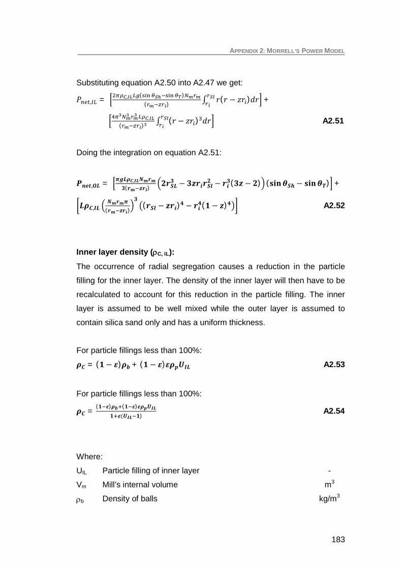
APPENDIX 2: MORRELL’S POWER MODEL
183
Substituting equation A2.50 into A2.47 we get:
= ( )( )
( ) +
( )( ) A2.51
Doing the integration on equation A2.51:
=( )
( ) ( ) +
( )( ) ( ) A2.52
Inner layer density ( C, IL):
The occurrence of radial segregation causes a reduction in the particle
filling for the inner layer. The density of the inner layer will then have to be
recalculated to account for this reduction in the particle filling. The inner
layer is assumed to be well mixed while the outer layer is assumed to
contain silica sand only and has a uniform thickness.
For particle fillings less than 100%:
= ( ) + ( ) A2.53
For particle fillings less than 100%:
=( ) ( )
) A2.54
Where:
UIL Particle filling of inner layer -
Vm Mill’s internal volume m3
b Density of balls kg/m3

APPENDIX 2: MORRELL’S POWER MODEL
184
p Density of silica particles kg/m3
Voidage (0.4) -
Inner layer particle filling (UIL):When segregation occurs, the volume of particles occupying the voids
between the balls in the inner layer reduces by an equivalent volume of
particles that have segregated to the outer layer. The new particle filling for
the inner layer will be:
= A2.55
Where:
VP, IL Volume of particles in the inner layer m3
Jb Ball filling -
Vm Mill’s internal volume m3
Voidage -
The volume of particles in the inner layer is the difference between the
total volume of particles in the mill (VP, Total) and the volume of particles in
the segregated outer layer (VP, OL).
A2.56
The total volume of particles present in the mill is given by:
( ) A2.57
The total volume of particles in the segregated layer has to be derived
from the geometry of the segregated layer. Considering Figure A2.5, the
charge is bound by sector OAB subtended by an angle The angle is
obtained by the difference between the toe and shoulder angular positions.

APPENDIX 2: MORRELL’S POWER MODEL
185
Figure A2.5: Morrell’s C model geometry
From the above geometry:
= ( ) A2.58
= ( ) A2.59
= (1
)( ) A2.60
The segregated layer radius (rSL) varies with mills speed and particle filling
increment. Thus
A2.61
Where:
s Radial segregation index -
Rinductive Inductive proximity probe’s measuring range (0.005m) m

APPENDIX 2: MORRELL’S POWER MODEL
186
Incorporating the definition of the segregated layer radius (equation A2.61)
into the definition of the volume of particles in the segregated layer
(equation A2.60) we obtain the following:
= ( )( ) A2.62
Looking back at the definition of particle filling in the inner layer (equation
A2.55) and incorporating the definitions for volume of particles in the inner
layer (equation A2.56) we then obtain:
=( )
A2.63
Thus including the definition of particle filling in the inner layer (equation
A2.63) into that of the density of the inner layer when segregation occurs
(equation A2.53 & A2.54); the density of the inner layer can be calculated.
The total net power for the charge will be given by:
+ A2.64

APPENDIX 2: MORRELL’S POWER MODEL
187
A2.4 POOL POWER MODELLING USING SIMPSON’SMETHOD
The pool shown in Figure A2.6 is assumed to contain only fine silica sand.
The symmetrical portion of the pool does not draw any power as the
torque from the two halves separated by the Y axis counter each other’s
effects. The additional mass shall only have an effect on the bearing
pressure. The particles present in the toe portion of the pool exert a
counter torque to the loads torque thus reducing its net torque and power
draw.
Figure A2.6: Illustration of the particle pool model

APPENDIX 2: MORRELL’S POWER MODEL
188
Assumptions:
The maximum load density occur at the particle filling (U) of 100%.
At this maximum density the void spaces between the balls are
completely filled with particles.
Pool formation begins at a particle filling greater than 100%. The
density of the load remains constant and maximum at particle filling
greater than 100%.
The pool consists of silica particles only
Coordinates defining the boundary of the pool:The coordinates defining the boundary of the toe portion of the particle
pool are p(XTP, YTP), T(XT, Rm, YT, Rm), (XTP, Ri, YTP, Ri) and (XT, Ri, YT, Ri) and
the indicated in Figure A2.6. The evaluations of the coordinates are:
Coordinates for the Toe, T
At the mill radius rm:
sin( )
cos( )
At the charge inner radius ri:
sin( )
cos( )
Coordinates for the pool, p:
At the mill radius rm:
= ( )
= tan
YT P: This is obtained by iterations of the pools height in the Simpsons
method when the calculated volume of the pool by the Simpsons

APPENDIX 2: MORRELL’S POWER MODEL
189
method is equal to the volume of the excess particles above a
particle filling of 100%.
At the charge inner radius ri:
= ( )
Assuming the particle pool’s surface is at the same level then:
=
Other important coordinates:
Minimum depth of the symmetrical pool: (0, ri)
Maximum height of the pool: (0, YTP)
Equation of the line through the origin and coordinates (XT, Rm, YT, Rm):
=
1. Calculation of the pool mass and volume:
For particle fillings greater than 100% the mass of particles present in the
pool is:
(1 ( % %) A2.65
Thus the volume of the pool will be:
( % %) A2.66
Where:
Jb Ball filling -
Vm Mill’s internal volume m3
UU>100% Fraction of particle filling greater than 100% -

APPENDIX 2: MORRELL’S POWER MODEL
190
UU=100% Fraction of particle filling at 100% -
Voidage -
p Particle density kg/m3
2. Calculation of the pools centre of gravity:
The volume of the pool calculated above combines the toe portion and the
symmetrical portion depending on the height of the pool. The toe portion of
the pool is responsible for the power loss. The centre of gravity that is
being calculated here is only for the toe portion of the pool. In Figure A2.6
the toe portion of the pool is divided into two sections, A and B. The
derivation of the pools centre of gravity is drawn up by considering these
two sections separately.
Centre of gravity of Section A:In Figure A2.6, consider an element of width b and length L in section A of
the toe portion of the particle pool. An exploded view of the element in
consideration can be viewed in Figure A2.7 below and is split into two
parts each having a mass m1 and m2.
Figure A2.7: Illustration of an element in the toe portion of the pool

APPENDIX 2: MORRELL’S POWER MODEL
191
Mass of the element
The mass of the rectangular section of the element is given by:
A2.67
The mass of the triangular section of the element is given by:
= ( ) A2.68
Thus the total mass of the element is given by given by the sum of
equations A2.27 and A2.68:
= ( ) A2.69
Generally for each element’s mass it can be expressed as:
= ( ) A2.70
Moment of the element about the Y – axis
The moment of the element is given by:
= A2.71
Using the dimensions of the element we obtain
=( )
( )A2.72
Simplifying equation A2.72 we get:
= ( )( )
A2.73
The moment about the Y-axis of each element in section A of the toe
portion of the pool (CXA, i) is given by the sum of the distance of an element
from the Y axis (XA, i) and the moment of the element. This is expressed
as:

APPENDIX 2: MORRELL’S POWER MODEL
192
+ [ ][ ] A2.74
The centre of gravity for section A is then given by:
= A2.75
Centre of gravity of Section B:In Figure A2.6, consider an element of width b and length L in section A of
the toe portion of the particle pool. An exploded view of the element in
consideration can be viewed in Figure A2.8 below and is split into two
parts each having a mass m1 and m2.
Figure A2.8: Illustration of an element in the toe portion of the pool
Mass of the element
The mass of the rectangular section of the element is given by:
A2.76
The mass of the triangular section of the element is given by:
= ( ) A2.77
Thus the total mass of the element is given by given by:

APPENDIX 2: MORRELL’S POWER MODEL
193
= ( ) A2.78
Generally for each element’s mass it can be expressed as:
= ( ) A2.79
Moment of the element about the Y – axis
The moment of the element about the Y – axis is given by:
= A2.80
Using the dimensions of the element we obtain
=( )
( )A2.81
Simplifying
= ( )( )
A2.82
The moment about the Y-axis of each element in section B of the toe
portion of the pool (CXB, i) is given by the sum of the distance of an element
from the Y axis (XB, i) and the moment of the element. This is expressed
as:
+ [ ][ ] A2.83
The centre of gravity for section B is then given by:
= A2.84
Thus the centre of gravity for the toe portion of the pool is given by:
= A2.85

APPENDIX 2: MORRELL’S POWER MODEL
194
Where:
=
=
3. Calculation of the pools torque and power
From the definition of torque:
A2.86
Thus the pools torque is given by:
= ( ) A2.87
The pools power is given by:
= A2.88

APPENDIX 2: MORRELL’S POWER MODEL
195
A2.5 MATLAB PROGRAM: POOL’S TORQUE AND POWER
%% Pool_Torq Program%% This program calculates the torque drawn by a pool in a batch ball mill%% using Numerical methods
clear allclc
%%Initialisation of variables
Ri = 0; Rm = 0.263; theta_T = 0; U = 0; Umax = 1; J = 0; Vm = 0; rho_P =0; X_TRm = 0; Y_TRm = 0; X_TRi = 0; Y_TRi = 0; del_U = 0; Mp = 0; Ep =0.4; Vpl = 0; Va = 0;Vb = 0; Vc = 0; Vd = 0; Ve = 0; Vf = 0; Vg = 0; Vh = 0;Vj = 0; a = 0.001; X_Tp = 0; X_Tl = 0; b = 0; n = 0; incr = 1; V_meas = 0;Vpool = 0; V_simp = 0; Y_even = 0; Y_odd = 0; Lm = 0; ind = 0; Y_Tp = 0;Y_Tp1 = 0; Ya_even = 0; Ya_odd = 0; Yb_even = 0; Yb_odd = 0; Yc_even= 0; Yc_odd = 0; Yd_even = 0; Yd_odd = 0;Ya = 0; Yb = 0;Yc = 0;
% User defined variablesRm = 0.263; %input('Enter value for the mill internal radius (meters) :');Lm = 0.18; %input('Enter value for the mill length (meters) :');Ri = 0.202811; %input('Enter value for the charge internal radius (meters):');N_rpm = 51.78444;theta_T = 137.2109; %input('Enter value for the toe`s angular position(degrees) :');U = 160/100; %(input('Enter value for the particle filling (%) :'))/100;J = 20/100; %(input('Enter value for the ball filling (%) :'))/100;Vm = 0.0387; %input('Enter value for the mills internal volume (m^3) :');rho_P = 2466.667; %input('Enter value for the particle density (kg/m^3) :');a = 0.0000001; %input('Enter value for the pool height (m) (Default =0.0001) :');n = 1000; %input('Enter number of strips to be created (default 1000) :');
%% Conversion of the toe coordinates of the load to cartesian coordinates
%Toe coordinates at the mill shellX_TRm = Rm*sin(pi-((pi/180)*theta_T));Y_TRm = Rm*cos(pi - ((pi/180)*theta_T));
%Toe coerdinates at the charge inner surface radiusX_TRi = Ri*sin(pi-((pi/180)*theta_T));Y_TRi = Ri*cos(pi - ((pi/180)*theta_T));
%% Calculation of the pools mass and volume

APPENDIX 2: MORRELL’S POWER MODEL
196
% Pool Massdel_U = U - Umax;Mp = Ep*(1 - Ep)*J*rho_P*Vm*del_U;
%Pool VolumeV_meas = 0.4*Ep*J*Vm*del_U; % Experimatally determined pool volumefrom particles filling
% Calculation of the pools volume% This is the first part of the calculation of the center of gravity of the% toe pool. The condition that has to be met when generating the pool is% that the Experimentally determined pool vulme V_meas should equalthe% pool volume generated by Simpson`s rule V_pool.
Y_Tp = Y_TRm; %Setting the pool height to be equal to the toe`s Y coord.
while (V_meas - Vpool) >= 0 %Dummy
Y_Tp = Y_Tp - a; % Increase the pool height
if Y_TRm >= Ri % Check if the symetrical pool is present
if Y_Tp >= Ri % Check if the symetrical pool is present
Ya_even = 0; Ya_odd = 0; Yb_even = 0; Yb_odd = 0;
X_Tp = sqrt((Rm^2)-(Y_Tp^2)); %Initial X coordinate of the pool X_Tl = (X_TRm/Y_TRm)*Y_Tp; % Final X coordinate of the pool
b = (X_Tp - X_TRm)/n; % Width of the strip for toe pool A c = (X_TRm - X_Tl)/n; % width of the strip for toe pool B
for k = 1:(n+1) % Loop to define the x coord and calc the%corresponding y coord
%Calculation of the Y coordinates of toe pool A Xa(k) = X_Tp - ((k-1)*b); % x coord of toe pool A Ya(k) = sqrt((Rm^2) - (Xa(k)^2)) - Y_Tp; % y coord of
%toe pool A

APPENDIX 2: MORRELL’S POWER MODEL
197
odd = ((k/2)-fix(k/2));
if (odd == 0)&(k ~= (n+1))&(k>1)% Sorts out and adds up%the Y coord with odd%indices excluding Y(1)% and Y(n)
Ya_even = Ya(k) + Ya_even;end
if (odd > 0)&(k ~= (n+1))&(k>1)% Sorts out and adds up%the Y coord with even%indices excluding Y(1)%and Y(n)
Ya_odd = Ya(k) + Ya_odd;end
% Calculation of the Y coordinate of toe pool B Xb(k) = X_TRm - ((k - 1)*c); % x coord of toe pool B Yb(k) = ((Y_TRm/X_TRm)*Xb(k)) - Y_Tp; % y coord of toepool B
odd = ((k/2)-fix(k/2));
if (odd == 0)&(k ~= (n+1))&(k>1)% Sorts out and adds up%the Y coord with odd%indices excluding Y(1) and Y(n)
Yb_even = Yb(k) + Yb_even;end
if (odd > 0)&(k ~= (n+1))&(k>1)% Sorts out and adds up%the Y coord with even%indices excluding Y(1) and Y(n)
Yb_odd = Yb(k) + Yb_odd;end
end
% Calculation of the pool volume by Simpsons Rule Va = b/3*Lm*((Ya(1)+Ya((n+1))) + (4*Ya_even)+(2*Ya_odd)); Vb = c/3*Lm*((Yb(1)+Yb((n+1))) + (4*Yb_even)+(2*Yb_odd));
end
if (Y_Tp < Ri)&(Y_Tp >= Y_TRi)
Ya_even = 0; Ya_odd = 0; Yb_even = 0;

APPENDIX 2: MORRELL’S POWER MODEL
198
Yb_odd = 0; Yc_even = 0; Yc_odd = 0;
X_Tp = sqrt((Rm^2)-(Y_Tp^2)); X_Tl = X_TRm/Y_TRm*Y_Tp; X_Sp = sqrt((Ri^2)-(Y_Tp^2));
b = (X_Tp - X_TRm)/n; c = (X_TRm - X_Tl)/n; f = X_Sp/n;
for k = 1:(n+1)
Xa(k) = X_Tp - ((k-1)*b); Ya(k) = sqrt((Rm^2)-(Xa(k)^2))-Y_Tp;
odd = ((k/2)-fix(k/2));
if (odd == 0)&(k ~= (n+1))&(k>1)% Sorts out and adds up%the Y coord with odd indices%excluding Y(1) and Y(n)
Ya_even = Ya(k) + Ya_even;end
if (odd > 0)&(k ~= (n+1))&(k>1)% Sorts out and adds up%the Y coord with even indices%excluding Y(1) and Y(n)
Ya_odd = Ya(k) + Ya_odd;end
Xb(k) = X_TRm - ((k-1)*c); Yb(k) = ((Y_TRm/X_TRm)*Xb(k)) - Y_Tp;
if (odd == 0)&(k ~= (n+1))&(k>1)% Sorts out and adds up%the Y coord with odd indices%excluding Y(1) and Y(n)
Yb_even = Yb(k) + Yb_even;end
if (odd > 0)&(k ~= (n+1))&(k>1)% Sorts out and adds up%the Y coord with even indices%excluding Y(1) and Y(n)
Yb_odd = Yb(k) + Yb_odd;end

APPENDIX 2: MORRELL’S POWER MODEL
199
Xc(k) = X_Sp - ((k-1)*f); Yc(k) = sqrt((Ri^2)-(Xc(k)^2))-Y_Tp;
if (odd == 0)&(k ~= (n+1))&(k>1)% Sorts out and adds up%the Y coord with odd indices%excluding Y(1) and Y(n)
Yc_even = Yc(k) + Yc_even;end
if (odd > 0)&(k ~= (n+1))&(k>1)% Sorts out and adds up%the Y coord with even indices%excluding Y(1) and Y(n)
Yc_odd = Yc(k) + Yc_odd;end
end
% Calculation of the pool volume using Simpson rule Va = b/3*Lm*((Ya(1)+Ya((n+1))) + (4*Ya_even)+(2*Ya_odd)); Vb = c/3*Lm*((Yb(1)+Yb((n+1))) + (4*Yb_even)+(2*Yb_odd)); Vc = 2*f/3*Lm*((Yc(1)+Yc((n+1)))+(4*Yc_even)+(2*Yc_odd));
end
if (Y_Tp < Y_TRi) & (Y_Tp >= 0)
Ya_even = 0; Ya_odd = 0; Yb_even = 0; Yb_odd = 0; Yc_even = 0; Yc_odd = 0; Yd_even = 0; Yd_odd = 0;
X_Tp = sqrt((Rm^2)-(Y_Tp^2)); X_Sp = sqrt((Ri^2) - (Y_Tp^2));
b = (X_Tp - X_TRm)/n; c = (X_TRm - X_TRi)/n; f = X_TRi/n; g = X_Sp/n;
for k = 1:(n+1)
Xa(k) = X_Tp - ((k-1)*b); Ya(k) = sqrt((Rm^2)-(Xa(k)^2))-Y_Tp;

APPENDIX 2: MORRELL’S POWER MODEL
200
odd = ((k/2)-fix(k/2));
if (odd == 0)&(k ~= (n+1))&(k>1)% Sorts out and adds up%the Y coord with odd indices% excluding Y(1) and Y(n)
Ya_even = Ya(k) + Ya_even;end
if (odd > 0)&(k ~= (n+1))&(k>1)% Sorts out and adds up%the Y coord with even indices%excluding Y(1) and Y(n)
Ya_odd = Ya(k) + Ya_odd;end
Xb(k) = X_TRm - ((k-1)*c); Yb(k) = (((Y_TRm/X_TRm)*Xb(k)) - Y_Tp);
if (odd == 0)&(k ~= (n+1))&(k>1)% Sorts out and adds up%the Y coord with odd indices%excluding Y(1) and Y(n)
Yb_even = Yb(k) + Yb_even;end
if (odd > 0)&(k ~= (n+1))&(k>1)% Sorts out and adds up%the Y coord with even indices%excluding Y(1) and Y(n)
Yb_odd = Yb(k) + Yb_odd;end
Xc(k) = X_TRi - ((k-1)*f); Yc(k) = sqrt((Ri^2)-(Xc(k)^2))-Y_Tp;
if (odd == 0)&(k ~= (n+1))&(k>1)% Sorts out and adds up%the Y coord with odd indices%excluding Y(1) and Y(n)
Yc_even = Yc(k) + Yc_even;
end
if (odd > 0)&(k ~= (n+1))&(k>1)% Sorts out and adds up%the Y coord with even indices%excluding Y(1) and Y(n)
Yc_odd = Yc(k) + Yc_odd;
end

APPENDIX 2: MORRELL’S POWER MODEL
201
Xd(k) = 0 - ((k-1)*g); Yd(k) = sqrt((Ri^2)-((Xd(k))^2))-Y_Tp;
if (odd == 0)&(k ~= (n+1))&(k>1)% Sorts out and adds up%the Y coord with odd indices%excluding Y(1) and Y(n)
Yd_even = Yd(k) + Yd_even;
end
if (odd > 0)&(k ~= (n+1))&(k>1)% Sorts out and adds up%the Y coord with even indices%excluding Y(1) and Y(n)
Yd_odd = Yd(k) + Yd_odd;
endend% Calculation of the pool volume using Simpson rule
Va = b/3*Lm*((Ya(1)+Ya(n+1)) + (4*Ya_even) + (2*Ya_odd)); Vb = c/3*Lm*((Yb(1)+Yb(n+1)) + (4*Yb_even) + (2*Yb_odd)); Vc = f/3*Lm*((Yc(1)+Yc(n+1)) + (4*Yc_even) + (2*Yc_odd)); Vd = g/3*Lm*((Yd(1)+Yd(n+1)) + (4*Yd_even) + (2*Yd_odd));
end
Vpool = Va + Vb+ Vc+ Vd;
elseif Y_TRm < Ri % If the Toe Pool is above the inner surface radius
if (Y_Tp >= Y_TRm) & (Y_Tp < Ri) % Is the pool height between% the toe Y coordinate and the% charge inner surface radius?
Ye_even = 0; Ye_odd = 0;
X_Sp = sqrt((Ri^2)-(Y_Tp^2)); h = X_Sp/n;
for k = 1:(n+1)
%Calculation of the Y coordinates of the pool Xe(k) = X_Sp - ((k-1)*h); Ye(k) = (sqrt((Ri^2)-(Xe(k)^2)))- Y_Tp;
odd = ((k/2)-fix(k/2));

APPENDIX 2: MORRELL’S POWER MODEL
202
if (odd == 0)&(k ~= (n+1))&(k>1)% Sorts out and adds up%the Y coord with odd indices% excluding Y(1) and Y(n)
Ye_even = Ye(k) + Ye_even;end
if (odd > 0)&(k ~= (n+1))&(k>1)% Sorts out and adds up%the Y coord with even indices%excluding Y(1) and Y(n)
Ye_odd = Ye(k) + Ye_odd;
endend% Calculation of the volume of the symetrical pool
Ve = 2*h/3*Lm*((Ye(1)+Ye(n+1))+(4*Ye_even)+(2*Ye_odd));end
if (Y_Tp < (Y_TRm-a)) %Is pool height greater than the%Y coordinate of the toe's angular position?
Ve = 0; Yf_even = 0; Yf_odd = 0; Yg_even = 0; Yg_odd = 0; Yh_even = 0; Yh_odd = 0; Yj_even = 0; Yj_odd = 0;
X_Tp = sqrt((Rm^2)-(Y_Tp^2)); X_Tl = (X_TRm/Y_TRm)*Y_Tp; X_Sp = sqrt((Ri^2)-(Y_Tp^2));
l = (X_Tp - X_TRm)/n; m = (X_TRm - X_Tl)/n; p = X_TRi/n; q = X_Sp/n;
for k = 1:(n+1)
% Calculations for toe pool A Xf(k) = X_Tp - ((k-1)*l); Yf(k) = sqrt((Rm^2)- (Xf(k)^2)) - Y_Tp;
odd = ((k/2)-fix(k/2));if (odd == 0)&(k ~= (n+1))&(k>1)% Sorts out and adds up

APPENDIX 2: MORRELL’S POWER MODEL
203
% the Y coord with odd indices% excluding Y(1) and Y(n)
Yf_even = Yf(k) + Yf_even;end
if (odd > 0)&(k ~= (n+1))&(k>1)% Sorts out and adds up% the Y coord with even indices% excluding Y(1) and Y(n)
Yf_odd = Yf(k) + Yf_odd;end
% Calculations for toe pool B Xg(k) = X_TRm - ((k-1)*m); Yg(k) = ((Y_TRm/ X_TRm)*Xg(k)) - Y_Tp;
if (odd == 0)&(k ~= (n+1))&(k>1)% Sorts out and adds up% the Y coord with odd indices% excluding Y(1) and Y(n)
Yg_even = Yg(k) + Yg_even;end
if (odd > 0)&(k ~= (n+1))&(k>1)% Sorts out and adds up% the Y coord with even indices% excluding Y(1) and Y(n)
Yg_odd = Yg(k) + Yg_odd;end
% Calculations for toe pool C Xh(k) = X_TRi - ((k-1)*p); Yh(k) = sqrt((Ri^2)- (Xh(k)^2)) - Y_Tp;
if (odd == 0)&(k ~= (n+1))&(k>1)% Sorts out and adds up% the Y coord with odd indices% excluding Y(1) and Y(n)
Yh_even = Yh(k) + Yh_even;end
if (odd > 0)&(k ~= (n+1))&(k>1)% Sorts out and adds up% the Y coord with even indices% excluding Y(1) and Y(n)
Yh_odd = Yh(k) + Yh_odd;end
% Calculations for toe pool D Xj(k) = 0 - ((k-1)*q); Yj(k) = sqrt((Ri^2)- (Xj(k)^2)) - Y_Tp;

APPENDIX 2: MORRELL’S POWER MODEL
204
if (odd == 0)&(k ~= (n+1))&(k>1)% Sorts out and adds up% the Y coord with odd indices% excluding Y(1) and Y(n)
Yj_even = Yj(k) + Yj_even;end
if (odd > 0)&(k ~= (n+1))&(k>1)% Sorts out and adds up% the Y coord with even indices% excluding Y(1) and Y(n)
Yj_odd = Yj(k) + Yj_odd;end
end
% Calculation of the pool volume using Simpson rule Vf = l/3*Lm*((Yf(1)+Yf(n+1)) + (4*Yf_even) + (2*Yf_odd)); Vg = m/3*Lm*((Yg(1)+Yg(n+1)) + (4*Yg_even) + (2*Yg_odd)); Vh = p/3*Lm*((Yh(1)+Yh(n+1)) + (4*Yh_even) + (2*Yh_odd)); Vj = q/3*Lm*((Yj(1)+Yj(n+1)) + (4*Yj_even) + (2*Yj_odd));
end
Vpool = Ve + Vf + Vg+ Vh + Vj;end
V_simp = Vpool;end
%%Calculation of the pools center of gravityif Y_Tp < Y_TRi
sum_MCx_r = 0; sum_MCx_s = 0; sum_MCx_t = 0;
X_Tpi = sqrt((Ri^2)-(Y_Tp^2));
for k = 1:(n+1)
% create strips for different regions of the toe pool r = (X_Tp - X_TRm)/n; s = (X_TRm - X_Tpi)/n; t = ((X_Tpi - X_TRi)/n);
% X & Y coordinates Xr(k) = X_Tp - ((k-1)*r); Yr(k) = sqrt((Rm^2)- (Xr(k)^2)) - Y_Tp;

APPENDIX 2: MORRELL’S POWER MODEL
205
Xs(k) = X_TRm - ((k-1)*s); Ys(k) = (Y_TRm/X_TRm*Xs(k)) - Y_Tp;
Xt(k) = X_Tpi - ((k-1)*t); Yt(k) = sqrt((Ri^2)-(Xt(k)^2)) - Y_Tp;
end
% Calculation of center of gravity for the strips
for k = 1:n
% Calculation of the centre of gravity for individual strips Cx_r(k) = (r*((2*Yr(k))+ (Yr(k+1)))/(3*(Yr(k)+Yr(k+1))))+ Xr(k+1); Cx_s(k) = (s*((2*Ys(k))+ (Ys(k+1)))/(3*(Ys(k)+Ys(k+1))))+ Xs(k+1); Cx_t(k) = (t*((2*Yt(k))+ (Yt(k+1)))/(3*(Yt(k)+Yt(k+1))))+ Xt(k+1);
%Calculation of the mass of the individual elements Mr(k) = 0.5*r*Lm*rho_P*(Yr(k)+Yr(k+1)); Ms(k) = 0.5*s*Lm*rho_P*(Ys(k)+Ys(k+1)); Mt(k) = 0.5*t*Lm*rho_P*(Yt(k)+Yt(k+1));
%Calculation of the product of Cx * M for individual strips sum_MCx_r = sum_MCx_r + (Mr(k)*Cx_r(k)); sum_MCx_s = sum_MCx_s + (Ms(k)*Cx_s(k)); sum_MCx_t = sum_MCx_t + (Mt(k)*Cx_t(k));
end
M_total = sum(Mr + Ms + Mt);% Total pool mass sum_MCx = sum_MCx_r + sum_MCx_s + sum_MCx_t; %Total sum ofthe product of M * Cx Cx = (sum_MCx/M_total)end
if Y_Tp >= Y_TRi
sum_MCx_u = 0; sum_MCx_v = 0;
X_Tpi = (X_TRm/Y_TRm)*Y_Tp;
for k = 1:(n+1)
% create strips for different regions of the toe pool u = (X_Tp - X_TRm)/n; v = (X_TRm - X_Tpi)/n;

APPENDIX 2: MORRELL’S POWER MODEL
206
% X & Y coordinates Xu(k) = X_Tp - ((k-1)*u); Yu(k) = sqrt((Rm^2)- (Xu(k)^2)) - Y_Tp;
Xv(k) = X_TRm - ((k-1)*v); Yv(k) = (Y_TRm/X_TRm*Xv(k)) - Y_Tp;
end
% Calculation of center of gravity for the stripsfor k = 1:n
% Calculation of the centre of gravity for individual strips Cx_u(k) = (u*((2*Yu(k))+ (Yu(k+1)))/(3*(Yu(k)+Yu(k+1))))+ Xu(k+1); Cx_v(k) = (v*((2*Yv(k))+ (Yv(k+1)))/(3*(Yv(k)+Yv(k+1))))+ Xv(k+1);
%Calculation of the mass of the individual elements Mu(k) = 0.5*u*Lm*rho_P*(Yu(k)+Yu(k+1)); Mv(k) = 0.5*v*Lm*rho_P*(Yv(k)+Yv(k+1));
%Calculation of the product of Cx * M for individual strips sum_MCx_u = sum_MCx_u + (Mu(k)*Cx_u(k)); sum_MCx_v = sum_MCx_v + (Mv(k)*Cx_v(k));
end
M_total = sum(Mu + Mv);% Total pool mass sum_MCx = sum_MCx_u + sum_MCx_v; %Total sum of the product ofM * Cx Cx = (sum_MCx/M_total)end
%% Pool Torque and Power calculationTorq = M_total*9.81*CxPower = 2*pi*N_rpm*Torq/60

APPENDIX 3
TORQUE AREM MODEL
A3

APPENDIX 3: TORQUE ARM MODEL
A3.1 REGRESSION ON BALLS ONLY DATA
Table A3.1: Parameter estimation for balls only loadParametersK 0.124
0.836J 2.935
N* 136.000N 1.018
Experiment DataMill Speed, N (%) 62.993 75.316 85.046 95.893 62.985 78.677 87.725 96.843Mill Speed, rpm 37.006 44.246 49.962 56.334 37.002 46.221 51.536 56.893Power, Watts 167.942 207.920 236.164 269.806 171.825 221.253 252.773 278.580StdDev 0.920 1.323 1.901 2.560 1.523 1.279 2.115 3.352Mill Filling, J (-) 0.200 0.200 0.200 0.200 0.200 0.200 0.200 0.200Internal Mill Diameter, D (m) 0.526 0.526 0.526 0.526 0.526 0.526 0.526 0.526Mill Length, L (m) 0.180 0.180 0.180 0.180 0.180 0.180 0.180 0.180Model DataBall Density, rb (Kg/m3) 7800.000 7800.000 7800.000 7800.000 7800.000 7800.000 7800.000 7800.000Load Density, rl (kg/m3) 4680.000 4680.000 4680.000 4680.000 4680.000 4680.000 4680.000 4680.000
c 0.000 0.000 0.000 0.000 0.000 0.000 0.000 0.000Thickness of centrifuged layer, mm 0.000 0.000 0.000 0.000 0.000 0.000 0.000 0.000Effective mill Diameter, Deff (m) 0.526 0.526 0.526 0.526 0.526 0.526 0.526 0.526Effective mill filling, Jeff (-) 0.200 0.200 0.200 0.200 0.200 0.200 0.200 0.200Effective Critical Mill Speed (RPM) 58.747 58.747 58.747 58.747 58.747 58.747 58.747 58.747Effective mill speed, Neff (%) 62.993 75.316 85.046 95.893 62.985 78.677 87.725 96.843Angle of repose, rads 0.785 0.785 0.785 0.785 0.785 0.785 0.785 0.785Angle of repose, degrees 45.000 45.000 45.000 45.000 45.000 45.000 45.000 45.000Model_Net Power (Watts) 176.779 211.362 238.670 269.109 176.757 220.795 246.187 271.775
(Expt - Mod) -8.837 -3.442 -2.506 0.697 -4.931 0.457 6.586 6.805SSE 210.927
Experiment 2Experiment 1

APPENDIX 3: TORQUE ARM MODEL
209
Figure A3.1: Model fit for balls only load

APPENDIX 3: TORQUE ARM MODEL
210
A3.2 REGRESSION ON POWER DATA FROM COARSE PARTICLE EXPERIMENTS
Table A3.2: Parameter estimation for coarse particles at the mill speed of 63% of the criticalParametersK 0.124
0.836J 2.935
N* 136.000N 1.018
Experiment DataParticle Filling, U (-) 0 20 40 60 70 80 90 100 110 150Power_Expt (Watts) 167.942 173.925 184.655 187.747 191.792 200.997 200.292 203.689 209.045 213.534StdDev 0.199 0.279 0.185 0.266 0.150 0.185 0.295 0.305 0.221 0.437Mill Speed (%) 63.468 63.468 63.468 63.468 63.468 63.468 63.468 63.468 63.468 63.468Mill Speed rpm 37.286 37.286 37.286 37.286 37.286 37.286 37.286 37.286 37.286 37.286Ball filling (J) 0.200 0.200 0.200 0.200 0.200 0.200 0.200 0.200 0.208 0.240Internal Mill Diameter, D (m) 0.526 0.526 0.526 0.526 0.526 0.526 0.526 0.526 0.526 0.526Mill Length, L (m) 0.180 0.180 0.180 0.180 0.180 0.180 0.180 0.180 0.180 0.180Ball Density (Kg/m3) 7800.000 7800.000 7800.000 7800.000 7800.000 7800.000 7800.000 7800.000 7800.000 7800.000Particle Density (Kg/m3) 2466.667 2466.667 2466.667 2466.667 2466.667 2466.667 2466.667 2466.667 2466.667 2466.667Load Density (kg/m3) 4680.000 4798.400 4916.800 5035.200 5094.400 5153.600 5212.800 5272.000 5126.154 4640.000Model DataN* 136.000 136.000 136.000 136.000 136.000 136.000 136.000 136.000 136.000 136.000N*f 136.000 136.000 136.000 136.000 136.000 136.000 136.000 136.000 136.000 136.000Ucrit 2.500 2.500 2.500 2.500 2.500 2.500 2.500 2.500 2.500 2.500N*p 136.000 136.000 136.000 136.000 136.000 136.000 136.000 136.000 136.000 136.000dc 0.000 0.000 0.000 0.000 0.000 0.000 0.000 0.000 0.000 0.000Thickness of centrifuged layer, mm 0.000 0.000 0.000 0.000 0.000 0.000 0.000 0.000 0.000 0.000Deff 0.526 0.526 0.526 0.526 0.526 0.526 0.526 0.526 0.526 0.526Jeff 0.200 0.200 0.200 0.200 0.200 0.200 0.200 0.200 0.208 0.240Nceff , (rpm) 58.747 58.747 58.747 58.747 58.747 58.747 58.747 58.747 58.747 58.747Neff , (%) 63.468 63.468 63.468 63.468 63.468 63.468 63.468 63.468 63.468 63.468a 0.785 0.785 0.785 0.785 0.785 0.785 0.785 0.785 0.785 0.785Power_Model (Watts) 178.378 182.891 187.404 191.917 194.173 196.430 198.686 200.943 201.566 203.698
(Expt - Mod) -10.436 -8.966 -2.749 -4.170 -2.381 4.567 1.606 2.746 7.479 9.836SSE 403.589

APPENDIX 3: TORQUE ARM MODEL
211
Table A3.3: Parameter estimation for coarse particles at the mill speed of 78% of the criticalParametersK 0.126
0.836J 2.935
N* 136.000N 1.018
Experiment DataParticle Filling, U (-) 0 20 40 60 70 80 90 100 110 150Power_Expt (Watts) 207.920 224.045 231.809 237.486 238.439 252.005 251.649 255.973 244.451 219.352StdDev 1.323 1.234 1.901 1.156 0.902 1.123 1.066 1.440 11.870 8.133Mill Speed (%) 77.784 77.784 77.784 77.784 77.784 77.784 77.784 77.784 77.784 77.784Mill Speed rpm 45.696 45.696 45.696 45.696 45.696 45.696 45.696 45.696 45.696 45.696Ball filling (J) 0.200 0.200 0.200 0.200 0.200 0.200 0.200 0.200 0.208 0.240Internal Mill Diameter, D (m) 0.526 0.526 0.526 0.526 0.526 0.526 0.526 0.526 0.526 0.526Mill Length, L (m) 0.180 0.180 0.180 0.180 0.180 0.180 0.180 0.180 0.180 0.180Ball Density (Kg/m3) 7800.000 7800.000 7800.000 7800.000 7800.000 7800.000 7800.000 7800.000 7800.000 7800.000Particle Density (Kg/m3) 2466.667 2466.667 2466.667 2466.667 2466.667 2466.667 2466.667 2466.667 2466.667 2466.667Load Density (kg/m3) 4680.000 4798.400 4916.800 5035.200 5094.400 5153.600 5212.800 5272.000 5126.154 4640.000Model DataN* 136.000 136.000 136.000 136.000 136.000 136.000 136.000 136.000 136.000 78.324N*f 78.324 78.324 78.324 78.324 78.324 78.324 78.324 78.324 78.324 78.324Ucrit 1.300 1.300 1.300 1.300 1.300 1.300 1.300 1.300 1.300 1.300N*p 136.000 136.000 136.000 136.000 136.000 136.000 136.000 136.000 136.000 78.324dc 0.000 0.000 0.000 0.000 0.000 0.000 0.000 0.000 0.000 0.009Thickness of centrifuged layer, mm 0.000 0.000 0.000 0.000 0.000 0.000 0.000 0.000 0.000 4.689Deff 0.526 0.526 0.526 0.526 0.526 0.526 0.526 0.526 0.526 0.517Jeff 0.200 0.200 0.200 0.200 0.200 0.200 0.200 0.200 0.208 0.212Nceff , (rpm) 58.747 58.747 58.747 58.747 58.747 58.747 58.747 58.747 58.747 59.288Neff , (%) 77.784 77.784 77.784 77.784 77.784 77.784 77.784 77.784 77.784 77.074a 0.785 0.785 0.785 0.785 0.785 0.785 0.785 0.785 0.785 0.785Power_Model (Watts) 220.993 226.584 232.175 237.766 240.561 243.357 246.152 248.948 249.720 218.271
(Expt - Mod) -13.073 -2.539 -0.366 -0.280 -2.122 8.648 5.497 7.026 -5.269 1.080SSE 365.366

APPENDIX 3: TORQUE ARM MODEL
212
Table A3.4: Power prediction with N* = 88 for coarse particles at the mill speed of 88% of the criticalParametersK 0.125
0.836J 2.935
N* 136.000
N 1.018
Experiment DataParticle Filling, U (-) 0 20 40 60 70 80 90 100 110 150Power_Expt (Watts) 236.164 258.624 264.437 275.737 269.589 253.047 243.850 230.850 215.696 238.643StdDev 1.901 1.277 3.001 1.725 3.755 4.603 1.599 3.674 2.156 7.241Mill Speed (%) 87.979 87.979 87.979 87.979 87.979 87.979 87.979 87.979 87.979 87.979Mill Speed rpm 51.685 51.685 51.685 51.685 51.685 51.685 51.685 51.685 51.685 51.685Ball filling (J) 0.200 0.200 0.200 0.200 0.200 0.200 0.200 0.200 0.208 0.240Internal Mill Diameter, D (m) 0.526 0.526 0.526 0.526 0.526 0.526 0.526 0.526 0.526 0.526Mill Length, L (m) 0.180 0.180 0.180 0.180 0.180 0.180 0.180 0.180 0.180 0.180Ball Density (Kg/m3) 7800.000 7800.000 7800.000 7800.000 7800.000 7800.000 7800.000 7800.000 7800.000 7800.000Particle Density (Kg/m3) 2466.667 2466.667 2466.667 2466.667 2466.667 2466.667 2466.667 2466.667 2466.667 2466.667Load Density (kg/m3) 4680.000 4798.400 4916.800 5035.200 5094.400 5153.600 5212.800 5272.000 5126.154 4640.000Model DataN* 136.000 136.000 136.000 136.000 136.000 88.000 88.000 88.000 88.000 88.000N*f 97.892 94.731 92.149 90.147 89.363 88.724 88.230 87.880 87.676 88.306Ucrit 0.750 0.750 0.750 0.750 0.750 0.750 0.750 0.750 0.750 0.750N*p 136.000 136.000 136.000 136.000 136.000 88.000 88.000 88.000 88.000 88.000
0.000 0.000 0.000 0.000 0.000 0.009 0.009 0.009 0.010 0.015Thickness of centrifuged layer, mm 0.000 0.000 0.000 0.000 0.000 4.573 4.573 4.573 5.131 7.809Deff 0.526 0.526 0.526 0.526 0.526 0.517 0.517 0.517 0.516 0.510Jeff 0.200 0.200 0.200 0.200 0.200 0.171 0.171 0.171 0.176 0.193Nceff , (rpm) 58.747 58.747 58.747 58.747 58.747 59.275 59.275 59.275 59.340 59.657Neff , (%) 87.979 87.979 87.979 87.979 87.979 87.196 87.196 87.196 87.100 86.637
0.785 0.785 0.785 0.785 0.785 0.785 0.785 0.785 0.785 0.785Power_Model (Watts) 249.382 255.691 262.000 268.309 271.464 230.507 233.155 235.803 233.100 220.552
(Expt - Mod) -13.218 2.933 2.436 7.428 -1.875 22.539 10.695 -4.953 -17.404 18.091SSE 1197.757

APPENDIX 3: TORQUE ARM MODEL
213
Table A3.5: N* linear model parameter estimation for coarse particles at the mill speed of 88% of the criticalParametersK 0.125
0.836
J 2.935N* 136.000
N 1.018N* Linear model parametersa1 -3.127b1 91.103Experiment DataParticle Filling, U (-) 0 20 40 60 70 80 90 100 110Power_Expt (Watts) 236.164 258.624 264.437 275.737 269.589 253.047 243.850 230.850 215.696StdDev 1.901 1.277 3.001 1.725 3.755 4.603 1.599 3.674 2.156Mill Speed (%) 87.979 87.979 87.979 87.979 87.979 87.979 87.979 87.979 87.979Mill Speed rpm 51.685 51.685 51.685 51.685 51.685 51.685 51.685 51.685 51.685Ball filling (J) 0.200 0.200 0.200 0.200 0.200 0.200 0.200 0.200 0.208Internal Mill Diameter, D (m) 0.526 0.526 0.526 0.526 0.526 0.526 0.526 0.526 0.526Mill Length, L (m) 0.180 0.180 0.180 0.180 0.180 0.180 0.180 0.180 0.180Ball Density (Kg/m3) 7800.000 7800.000 7800.000 7800.000 7800.000 7800.000 7800.000 7800.000 7800.000Particle Density (Kg/m3) 2466.667 2466.667 2466.667 2466.667 2466.667 2466.667 2466.667 2466.667 2466.667Load Density (kg/m3) 4680.000 4798.400 4916.800 5035.200 5094.400 5153.600 5212.800 5272.000 5126.154Model DataN* 136.000 136.000 136.000 136.000 136.000 88.601 88.289 87.976 87.663N*f 97.892 94.731 92.149 90.147 89.363 88.724 88.230 87.880 87.676Ucrit 0.750 0.750 0.750 0.750 0.750 0.750 0.750 0.750 0.750N*p 136.000 136.000 136.000 136.000 136.000 88.601 88.289 87.976 87.663
c 0.000 0.000 0.000 0.000 0.000 0.005 0.007 0.009 0.014Thickness of centrifuged layer, mm 0.000 0.000 0.000 0.000 0.000 2.532 3.443 4.682 7.142Deff 0.526 0.526 0.526 0.526 0.526 0.521 0.519 0.517 0.512Jeff 0.200 0.200 0.200 0.200 0.200 0.184 0.179 0.171 0.163Nceff , (rpm) 58.747 58.747 58.747 58.747 58.747 59.038 59.143 59.288 59.578Neff , (%) 87.979 87.979 87.979 87.979 87.979 87.546 87.390 87.177 86.752
(Radians) 0.785 0.785 0.785 0.785 0.785 0.785 0.785 0.785 0.785Power_Model (Watts) 249.382 255.691 262.000 268.309 271.464 250.233 244.210 234.726 213.892
(Expt - Mod) -13.218 2.933 2.436 7.428 -1.875 2.814 -0.360 -3.877 1.804SSE 274.266

APPENDIX 3: TORQUE ARM MODEL
214
Table A3.6: N* linear model parameter estimation for coarse particles at the mill speed of 88% of the criticalParametersK 0.125
0.836
J 2.935N* 136.000
N 1.018
N* Linear model parametersa1 -3.127b1 91.103N* Linear model parametersa2 1.598b2 85.910Experiment DataParticle Filling, U (-) 0 20 40 60 70 80 90 100 110 150Power_Expt (Watts) 236.164 258.624 264.437 275.737 269.589 253.047 243.850 230.850 215.696 238.643StdDev 1.901 1.277 3.001 1.725 3.755 4.603 1.599 3.674 2.156 7.241Mill Speed (%) 87.979 87.979 87.979 87.979 87.979 87.979 87.979 87.979 87.979 87.979Mill Speed rpm 51.685 51.685 51.685 51.685 51.685 51.685 51.685 51.685 51.685 51.685Ball filling (J) 0.200 0.200 0.200 0.200 0.200 0.200 0.200 0.200 0.208 0.240Internal Mill Diameter, D (m) 0.526 0.526 0.526 0.526 0.526 0.526 0.526 0.526 0.526 0.526Mill Length, L (m) 0.180 0.180 0.180 0.180 0.180 0.180 0.180 0.180 0.180 0.180Ball Density (Kg/m3) 7800.000 7800.000 7800.000 7800.000 7800.000 7800.000 7800.000 7800.000 7800.000 7800.000Particle Density (Kg/m3) 2466.667 2466.667 2466.667 2466.667 2466.667 2466.667 2466.667 2466.667 2466.667 2466.667Load Density (kg/m3) 4680.000 4798.400 4916.800 5035.200 5094.400 5153.600 5212.800 5272.000 5126.154 4640.000Model DataN* 136.000 136.000 136.000 136.000 136.000 88.601 88.289 87.976 87.663 88.307N*f 97.892 94.731 92.149 90.147 89.363 88.724 88.230 87.880 87.676 88.306Ucrit 0.750 0.750 0.750 0.750 0.750 0.750 0.750 0.750 0.750 0.750N*p 136.000 136.000 136.000 136.000 136.000 88.601 88.289 87.976 87.663 88.307dc 0.000 0.000 0.000 0.000 0.000 0.005 0.007 0.009 0.014 0.011Thickness of centrifuged layer, mm 0.000 0.000 0.000 0.000 0.000 2.532 3.443 4.682 7.142 5.778Deff 0.526 0.526 0.526 0.526 0.526 0.521 0.519 0.517 0.512 0.514Jeff 0.200 0.200 0.200 0.200 0.200 0.184 0.179 0.171 0.163 0.205Nceff , (rpm) 58.747 58.747 58.747 58.747 58.747 59.038 59.143 59.288 59.578 59.416Neff , (%) 87.979 87.979 87.979 87.979 87.979 87.546 87.390 87.177 86.752 86.988a 0.785 0.785 0.785 0.785 0.785 0.785 0.785 0.785 0.785 0.785Power_Model (Watts) 249.382 255.691 262.000 268.309 271.464 250.233 244.210 234.726 213.892 237.330
(Expt - Mod) -13.218 2.933 2.436 7.428 -1.875 2.814 -0.360 -3.877 1.804 1.312SSE 274.266

APPENDIX 3: TORQUE ARM MODEL
215
Table A3.7: Power prediction with N* = 98 for coarse particles at the mill speed of 98% of the critical
ParametersK 0.126
0.937J 2.935
N* 136.000N 1.018
Experiment DataParticle Filling, U (-) 0 20 40 60 70 80 90 100 110 150Power_Expt (Watts) 269.806 290.506 289.874 288.930 264.318 251.065 237.848 226.363 233.843 235.896StdDev 2.560 2.184 1.654 2.543 9.285 5.648 5.332 11.246 5.001 4.975Mill Speed (%) 98.300 98.300 98.300 98.300 98.300 98.300 98.300 98.300 98.300 98.300Mill Speed rpm 57.749 57.749 57.749 57.749 57.749 57.749 57.749 57.749 57.749 57.749Ball filling (J) 0.200 0.200 0.200 0.200 0.200 0.200 0.200 0.200 0.208 0.240Internal Mill Diameter, D (m) 0.526 0.526 0.526 0.526 0.526 0.526 0.526 0.526 0.526 0.526Mill Length, L (m) 0.180 0.180 0.180 0.180 0.180 0.180 0.180 0.180 0.180 0.180Ball Density (Kg/m3) 7800.000 7800.000 7800.000 7800.000 7800.000 7800.000 7800.000 7800.000 7800.000 7800.000Particle Density (Kg/m3) 2466.667 2466.667 2466.667 2466.667 2466.667 2466.667 2466.667 2466.667 2466.667 2466.667Load Density (kg/m3) 4680.000 4798.400 4916.800 5035.200 5094.400 5153.600 5212.800 5272.000 5126.154 4640.000Model DataN* 136.000 136.000 136.000 136.000 98.000 98.000 98.000 98.000 98.000 98.000N*f 102.860 101.257 99.957 98.959 98.574 98.264 98.030 97.872 97.789 98.215Ucrit 0.650 0.650 0.650 0.650 0.650 0.650 0.650 0.650 0.650 0.650N*p 136.000 136.000 136.000 135.775 98.000 98.000 98.000 98.000 98.000 98.000dc 0.000 0.000 0.000 0.000 0.012 0.012 0.012 0.012 0.013 0.020Thickness of centrifuged layer, mm 0.000 0.000 0.000 0.000 6.271 6.271 6.271 6.271 7.036 10.709Deff 0.526 0.526 0.526 0.526 0.513 0.513 0.513 0.513 0.512 0.505Jeff 0.200 0.200 0.200 0.200 0.160 0.160 0.160 0.160 0.164 0.174Nceff , (rpm) 58.747 58.747 58.747 58.747 59.474 59.474 59.474 59.474 59.565 60.006Neff , (%) 98.300 98.300 98.300 98.300 97.098 97.098 97.098 97.098 96.950 96.238a 0.785 0.785 0.785 0.785 0.785 0.785 0.785 0.785 0.785 0.785Power_Model (Watts) 273.381 280.297 287.214 294.130 233.252 235.962 238.673 241.383 236.809 216.213
(Expt - Mod) -3.575 10.209 2.660 -5.200 31.066 15.103 -0.825 -15.020 -2.966 19.683SSE 1966.854

APPENDIX 3: TORQUE ARM MODEL
216
Table A3.8: N* linear model parameter estimation for coarse particles at the mill speed of 98% of the critical
ParametersK 0.126
0.937J 2.935
N* 136.000N 1.018
N* Linear model parametersa1 -0.059b1 98.186Experiment DataParticle Filling, U (-) 0 20 40 60 70 80 90 100 110 150Power_Expt (Watts) 269.806 290.506 289.874 288.930 264.318 251.065 237.848 226.363 233.843 235.896StdDev 2.560 2.184 1.654 2.543 9.285 5.648 5.332 11.246 5.001 4.975Mill Speed (%) 98.300 98.300 98.300 98.300 98.300 98.300 98.300 98.300 98.300 98.300Mill Speed rpm 57.749 57.749 57.749 57.749 57.749 57.749 57.749 57.749 57.749 57.749Ball filling (J) 0.200 0.200 0.200 0.200 0.200 0.200 0.200 0.200 0.208 0.240Internal Mill Diameter, D (m) 0.526 0.526 0.526 0.526 0.526 0.526 0.526 0.526 0.526 0.526Mill Length, L (m) 0.180 0.180 0.180 0.180 0.180 0.180 0.180 0.180 0.180 0.180Ball Density (Kg/m3) 7800.000 7800.000 7800.000 7800.000 7800.000 7800.000 7800.000 7800.000 7800.000 7800.000Particle Density (Kg/m3) 2466.667 2466.667 2466.667 2466.667 2466.667 2466.667 2466.667 2466.667 2466.667 2466.667Load Density (kg/m3) 4680.000 4798.400 4916.800 5035.200 5094.400 5153.600 5212.800 5272.000 5126.154 4640.000Model DataN* 136.000 136.000 136.000 135.775 98.145 98.139 98.133 98.127 98.121 98.098N*f 102.860 101.257 99.957 98.959 98.574 98.264 98.030 97.872 97.789 98.215Ucrit 0.650 0.650 0.650 0.650 0.650 0.650 0.650 0.650 0.650 0.650N*p 136.000 136.000 136.000 135.775 98.145 98.139 98.133 98.127 98.121 98.098dc 0.000 0.000 0.000 0.000 0.010 0.010 0.010 0.011 0.012 0.018Thickness of centrifuged layer, mm 0.000 0.000 0.000 0.000 5.440 5.471 5.503 5.535 6.246 9.729Deff 0.526 0.526 0.526 0.526 0.515 0.515 0.515 0.515 0.514 0.507Jeff 0.200 0.200 0.200 0.200 0.166 0.166 0.165 0.165 0.169 0.180Nceff , (rpm) 58.747 58.747 58.747 58.747 59.377 59.380 59.384 59.388 59.472 59.887Neff , (%) 98.300 98.300 98.300 98.300 97.258 97.252 97.246 97.240 97.103 96.429a 0.785 0.785 0.785 0.785 0.785 0.785 0.785 0.785 0.785 0.785Power_Model (Watts) 273.381 280.297 287.214 294.130 241.867 244.347 246.818 249.279 244.956 224.970
(Expt - Mod) -3.575 10.209 2.660 -5.200 22.451 6.718 -8.970 -22.916 -11.113 10.926SSE 1548.808

APPENDIX 3: TORQUE ARM MODEL
217
Table A3.9: N* linear model parameter estimation for coarse particles at the mill speed of 98% of the critical
ParametersK 0.126
0.937
J 2.935N* 136.000
N 1.018N* Linear model parameters - Cataractinga1 -2.597b1 100.359N* Linear model parameters - Centrifuginga2 0.690b2 97.189Experiment DataParticle Filling, U (-) 0 20 40 60 70 80 90 100 110 150Power_Expt (Watts) 269.806 290.506 289.874 288.930 264.318 251.065 237.848 226.363 233.843 235.896StdDev 2.560 2.184 1.654 2.543 9.285 5.648 5.332 11.246 5.001 4.975Mill Speed (%) 98.300 98.300 98.300 98.300 98.300 98.300 98.300 98.300 98.300 98.300Mill Speed rpm 57.749 57.749 57.749 57.749 57.749 57.749 57.749 57.749 57.749 57.749Ball filling (J) 0.200 0.200 0.200 0.200 0.200 0.200 0.200 0.200 0.208 0.240Internal Mill Diameter, D (m) 0.526 0.526 0.526 0.526 0.526 0.526 0.526 0.526 0.526 0.526Mill Length, L (m) 0.180 0.180 0.180 0.180 0.180 0.180 0.180 0.180 0.180 0.180Ball Density (Kg/m3) 7800.000 7800.000 7800.000 7800.000 7800.000 7800.000 7800.000 7800.000 7800.000 7800.000Particle Density (Kg/m3) 2466.667 2466.667 2466.667 2466.667 2466.667 2466.667 2466.667 2466.667 2466.667 2466.667Load Density (kg/m3) 4680.000 4798.400 4916.800 5035.200 5094.400 5153.600 5212.800 5272.000 5126.154 4640.000Model DataN* 136.000 136.000 136.000 135.775 98.541 98.282 98.022 97.762 97.947 98.223N*f 102.860 101.257 99.957 98.959 98.574 98.264 98.030 97.872 97.789 98.215Ucrit 0.650 0.650 0.650 0.650 0.650 0.650 0.650 0.650 0.650 0.650N*p 136.000 136.000 136.000 135.775 98.541 98.282 98.022 97.762 97.947 98.223dc 0.000 0.000 0.000 0.000 0.007 0.009 0.012 0.015 0.014 0.016Thickness of centrifuged layer, mm 0.000 0.000 0.000 0.000 3.685 4.756 6.138 7.922 7.411 8.601Deff 0.526 0.526 0.526 0.526 0.519 0.516 0.514 0.510 0.511 0.509Jeff 0.200 0.200 0.200 0.200 0.177 0.170 0.161 0.150 0.161 0.188Nceff , (rpm) 58.747 58.747 58.747 58.747 59.171 59.296 59.459 59.670 59.610 59.752Neff , (%) 98.300 98.300 98.300 98.300 97.596 97.390 97.124 96.779 96.878 96.648a 0.785 0.785 0.785 0.785 0.785 0.785 0.785 0.785 0.785 0.785Power_Model (Watts) 274.425 281.368 288.310 295.253 260.957 252.788 241.002 224.448 233.826 235.908
(Expt - Mod) -4.619 9.139 1.563 -6.323 3.361 -1.723 -3.154 1.915 0.017 -0.012SSE 175.150

APPENDIX 3: TORQUE ARM MODEL
218
A3.3 REGRESSION ON POWER DATA FROM FINE PARTICLE EXPERIMENTS
Table A3.10: Power prediction with N* = 64 for fine particles at the mill speed of 63% of the criticalParametersK 0.098
0.836J 2.935
N* 136.000N 1.018
Experiment DataParticle Filling, U (-) 0 20 40 60 70 80 90 100 110 120 160Power_Expt (Watts) 167.942 181.698 181.433 184.189 189.021 183.122 185.710 177.801 176.412 175.613 178.132StdDev 0.920 1.065 2.200 1.202 3.081 1.886 1.086 1.525 2.211 1.426 1.714Mill Speed (%) 63.335 63.335 63.335 63.335 63.335 63.335 63.335 63.335 63.335 63.335 63.335Mill Speed rpm 37.207 37.207 37.207 37.207 37.207 37.207 37.207 37.207 37.207 37.207 37.207Ball filling (J) 0.200 0.200 0.200 0.200 0.200 0.200 0.200 0.200 0.208 0.240 0.240Internal Mill Diameter, D (m) 0.526 0.526 0.526 0.526 0.526 0.526 0.526 0.526 0.526 0.526 0.526Mill Length, L (m) 0.180 0.180 0.180 0.180 0.180 0.180 0.180 0.180 0.180 0.180 0.180Ball Density (Kg/m3) 7800.000 7800.000 7800.000 7800.000 7800.000 7800.000 7800.000 7800.000 7800.000 7800.000 7800.000Particle Density (Kg/m3) 2466.667 2466.667 2466.667 2466.667 2466.667 2466.667 2466.667 2466.667 2466.667 2466.667 2466.667Load Density (kg/m3) 4680.000 4798.400 4916.800 5035.200 5094.400 5153.600 5212.800 5272.000 5126.154 4991.111 4538.065Model DataN* 136.000 136.000 136.000 136.000 136.000 136.000 136.000 64.000 64.000 64.000 64.000dc 0.000 0.000 0.000 0.000 0.000 0.000 0.000 0.005 0.005 0.008 0.008Thickness of centrifuged layer, mm 0.000 0.000 0.000 0.000 0.000 0.000 0.000 2.429 2.725 4.147 4.147Deff 0.526 0.526 0.526 0.526 0.526 0.526 0.526 0.521 0.521 0.518 0.518Jeff 0.200 0.200 0.200 0.200 0.200 0.200 0.200 0.185 0.191 0.216 0.248Nceff , (rpm) 58.747 58.747 58.747 58.747 58.747 58.747 58.747 59.026 59.060 59.225 59.225Neff , (%) 63.335 63.335 63.335 63.335 63.335 63.335 63.335 63.036 62.999 62.824 62.824a 0.785 0.785 0.785 0.785 0.785 0.785 0.785 0.785 0.785 0.785 0.785Power_Model (Watts) 170.711 175.030 179.349 183.667 185.827 187.986 190.146 176.421 175.782 185.898 187.725
(Expt - Mod) -2.769 6.668 2.085 0.521 3.194 -4.864 -4.435 1.380 0.630 -10.285 -9.593SSE 310.381

APPENDIX 3: TORQUE ARM MODEL
219
Table A3.11: N* linear model parameter estimation for fine particles at the mill speed of 63% of the criticalParametersK 0.098
0.836J 2.935
N* 136.000N 1.018
N* Linear model parametersa -1.583b 65.630Experiment DataParticle Filling, U (-) 0 20 40 60 70 80 90 100 110 120 160Power_Expt (Watts) 167.942 181.698 181.433 184.189 189.021 183.122 185.710 177.801 176.412 175.613 178.132StdDev 0.920 1.065 2.200 1.202 3.081 1.886 1.086 1.525 2.211 1.426 1.714Mill Speed (%) 63.335 63.335 63.335 63.335 63.335 63.335 63.335 63.335 63.335 63.335 63.335Mill Speed rpm 37.207 37.207 37.207 37.207 37.207 37.207 37.207 37.207 37.207 37.207 37.207Ball filling (J) 0.200 0.200 0.200 0.200 0.200 0.200 0.200 0.200 0.208 0.240 0.240Internal Mill Diameter, D (m) 0.526 0.526 0.526 0.526 0.526 0.526 0.526 0.526 0.526 0.526 0.526Mill Length, L (m) 0.180 0.180 0.180 0.180 0.180 0.180 0.180 0.180 0.180 0.180 0.180Ball Density (Kg/m3) 7800.000 7800.000 7800.000 7800.000 7800.000 7800.000 7800.000 7800.000 7800.000 7800.000 7800.000Particle Density (Kg/m3) 2466.667 2466.667 2466.667 2466.667 2466.667 2466.667 2466.667 2466.667 2466.667 2466.667 2466.667Load Density (kg/m3) 4680.000 4798.400 4916.800 5035.200 5094.400 5153.600 5212.800 5272.000 5126.154 4991.111 4538.065Model DataN* 136.000 136.000 136.000 136.000 136.000 136.000 136.000 64.047 63.889 63.731 63.098
0.000 0.000 0.000 0.000 0.000 0.000 0.000 0.004 0.006 0.010 0.019Thickness of centrifuged layer, mm 0.000 0.000 0.000 0.000 0.000 0.000 0.000 2.318 3.038 5.402 10.063Deff 0.526 0.526 0.526 0.526 0.526 0.526 0.526 0.521 0.520 0.515 0.506Jeff 0.200 0.200 0.200 0.200 0.200 0.200 0.200 0.186 0.189 0.216 0.248Nceff , (rpm) 58.747 58.747 58.747 58.747 58.747 58.747 58.747 59.013 59.096 59.372 59.928Neff , (%) 63.335 63.335 63.335 63.335 63.335 63.335 63.335 63.049 62.961 62.668 62.087
0.785 0.785 0.785 0.785 0.785 0.785 0.785 0.785 0.785 0.785 0.785Power_Model (Watts) 170.711 175.030 179.349 183.667 185.827 187.986 190.146 177.148 173.801 183.644 177.142
(Expt - Mod) -2.769 6.668 2.085 0.521 3.194 -4.864 -4.435 0.653 2.611 -8.031 0.990SSE 183.000

APPENDIX 3: TORQUE ARM MODEL
220
Table A3.12: Power prediction with N* = 78.98 for fine particles at the mill speed of 78% of the criticalParametersK 0.101
0.836J 2.935
N* 136.000N 1.018
Experiment DataParticle Filling, U (-) 0 20 40 60 70 80 90 100 110 160Power_Expt (Watts) 207.920 224.555 233.800 240.151 238.960 232.540 241.144 236.123 226.994 229.293StdDev 1.323 1.152 1.061 1.491 1.094 1.477 1.578 1.193 1.270 1.508Mill Speed (%) 78.064 78.064 78.064 78.064 78.064 78.064 78.064 78.064 78.064 78.064Mill Speed rpm 45.860 45.860 45.860 45.860 45.860 45.860 45.860 45.860 45.860 45.860Ball filling (J) 0.200 0.200 0.200 0.200 0.200 0.200 0.200 0.200 0.208 0.240Internal Mill Diameter, D (m) 0.526 0.526 0.526 0.526 0.526 0.526 0.526 0.526 0.526 0.526Mill Length, L (m) 0.180 0.180 0.180 0.180 0.180 0.180 0.180 0.180 0.180 0.180Ball Density (Kg/m3) 7800.000 7800.000 7800.000 7800.000 7800.000 7800.000 7800.000 7800.000 7800.000 7800.000Particle Density (Kg/m3) 2466.667 2466.667 2466.667 2466.667 2466.667 2466.667 2466.667 2466.667 2466.667 2466.667Load Density (kg/m3) 4680.000 4798.400 4916.800 5035.200 5094.400 5153.600 5212.800 5272.000 5126.154 4538.065Model DataN* 136.000 136.000 136.000 136.000 136.000 136.000 136.000 78.983 78.983 78.983dc 0.000 0.000 0.000 0.000 0.000 0.000 0.000 0.004 0.004 0.006Thickness of centrifuged layer, mm 0.000 0.000 0.000 0.000 0.000 0.000 0.000 1.893 2.124 3.232Deff 0.526 0.526 0.526 0.526 0.526 0.526 0.526 0.522 0.522 0.520Jeff 0.200 0.200 0.200 0.200 0.200 0.200 0.200 0.188 0.195 0.248Nceff , (rpm) 58.747 58.747 58.747 58.747 58.747 58.747 58.747 58.964 58.991 59.119Neff , (%) 78.064 78.064 78.064 78.064 78.064 78.064 78.064 77.777 77.742 77.573
0.785 0.785 0.785 0.785 0.785 0.785 0.785 0.785 0.785 0.785Power_Model (Watts) 217.206 222.701 228.196 233.691 236.439 239.186 241.934 228.948 228.485 240.979
(Expt - Mod) -9.286 1.854 5.604 6.460 2.522 -6.646 -0.790 7.175 -1.490 -11.686SSE 404.221

APPENDIX 3: TORQUE ARM MODEL
221
Table A3.13: N* linear model parameter estimation for fine particles at the mill speed of 78% of the criticalParametersK 0.101372
0.836413J 2.935335
N* 136N 1.017754
N* Linear model parametersa -2.13729b 81.4188Experiment DataParticle Filling, U (-) 0 20 40 60 70 80 90 100 110 160Power_Expt (Watts) 207.92 224.5554 233.8003 240.151 238.9604 232.5403 241.1444 236.1229 226.9944 229.2931StdDev 1.323088 1.15194 1.0609 1.491424 1.094196 1.477159 1.577637 1.192754 1.269668 1.508451Mill Speed (%) 78.06385 78.06385 78.06385 78.06385 78.06385 78.06385 78.06385 78.06385 78.06385 78.06385Mill Speed rpm 45.86037 45.86037 45.86037 45.86037 45.86037 45.86037 45.86037 45.86037 45.86037 45.86037Ball filling (J) 0.2 0.2 0.2 0.2 0.2 0.2 0.2 0.2 0.208 0.24Internal Mill Diameter, D (m) 0.526 0.526 0.526 0.526 0.526 0.526 0.526 0.526 0.526 0.526Mill Length, L (m) 0.18 0.18 0.18 0.18 0.18 0.18 0.18 0.18 0.18 0.18Ball Density (Kg/m3) 7800 7800 7800 7800 7800 7800 7800 7800 7800 7800Particle Density (Kg/m3) 2466.667 2466.667 2466.667 2466.667 2466.667 2466.667 2466.667 2466.667 2466.667 2466.667Load Density (kg/m3) 4680 4798.4 4916.8 5035.2 5094.4 5153.6 5212.8 5272 5126.154 4538.065Model DataN* 136 136 136 136 136 136 136 79.28151 79.06778 77.99913dc 1.68E-27 1.68E-27 1.68E-27 1.68E-27 1.68E-27 1.68E-27 1.68E-27 0.002683 0.003714 0.016156Thickness of centrifuged layer, mm 8.85E-25 8.85E-25 8.85E-25 8.85E-25 8.85E-25 8.85E-25 8.85E-25 1.411485 1.953787 8.497939Deff 0.526 0.526 0.526 0.526 0.526 0.526 0.526 0.523177 0.522092 0.509004Jeff 0.2 0.2 0.2 0.2 0.2 0.2 0.2 0.191343 0.1961 0.248Nceff , (rpm) 58.74726 58.74726 58.74726 58.74726 58.74726 58.74726 58.74726 58.90862 58.97097 59.73934Neff , (%) 78.06385 78.06385 78.06385 78.06385 78.06385 78.06385 78.06385 77.85002 77.76771 76.76746a 0.785398 0.785398 0.785398 0.785398 0.785398 0.785398 0.785398 0.785398 0.785398 0.785398Power_Model (Watts) 217.2058 222.701 228.1961 233.6912 236.4388 239.1863 241.9339 232.9587 229.8455 228.9054
(Expt - Mod) -9.28588 1.85438 5.604171 6.459741 2.521644 -6.64607 -0.78951 3.164181 -2.85104 0.387671SSE 232.2444

APPENDIX 3: TORQUE ARM MODEL
222
Table A3.14: Power prediction with N* = 89.2 for fine particles at the mill speed of 88% of the criticalParametersK 0.103
0.836J 2.935
N* 136.000N 1.018
Experiment DataParticle Filling, U (-) 0 20 40 60 70 80 90 100 110 120 160Power_Expt (Watts) 236.164 262.164 273.872 270.353 270.558 274.481 278.230 271.934 265.691 266.807 255.828StdDev 1.901 1.855 3.315 4.083 2.660 1.835 2.833 3.738 2.261 2.534 3.524Mill Speed (%) 88.144 88.144 88.144 88.144 88.144 88.144 88.144 88.144 88.144 88.144 88.144Mill Speed rpm 51.782 51.782 51.782 51.782 51.782 51.782 51.782 51.782 51.782 51.782 51.782Ball filling (J) 0.200 0.200 0.200 0.200 0.200 0.200 0.200 0.200 0.208 0.218 0.240Internal Mill Diameter, D (m) 0.526 0.526 0.526 0.526 0.526 0.526 0.526 0.526 0.526 0.526 0.526Mill Length, L (m) 0.180 0.180 0.180 0.180 0.180 0.180 0.180 0.180 0.180 0.180 0.180Ball Density (Kg/m3) 7800.000 7800.000 7800.000 7800.000 7800.000 7800.000 7800.000 7800.000 7800.000 7800.000 7800.000Particle Density (Kg/m3) 2466.667 2466.667 2466.667 2466.667 2466.667 2466.667 2466.667 2466.667 2466.667 2466.667 2466.667Load Density (kg/m3) 4680.000 4798.400 4916.800 5035.200 5094.400 5153.600 5212.800 5272.000 5126.154 4991.111 4538.065Model DataN* 136.000 136.000 136.000 136.000 136.000 136.000 136.000 89.166 89.166 89.166 89.166
c 0.000 0.000 0.000 0.000 0.000 0.000 0.000 0.003 0.004 0.004 0.006Thickness of centrifuged layer, mm 0.000 0.000 0.000 0.000 0.000 0.000 0.000 1.711 1.920 2.203 2.922Deff 0.526 0.526 0.526 0.526 0.526 0.526 0.526 0.523 0.522 0.522 0.520Jeff 0.200 0.200 0.200 0.200 0.200 0.200 0.200 0.189 0.196 0.205 0.240Nceff , (rpm) 58.747 58.747 58.747 58.747 58.747 58.747 58.747 58.943 58.967 59.000 59.083Neff , (%) 88.144 88.144 88.144 88.144 88.144 88.144 88.144 87.851 87.815 87.767 87.643
(Radians) 0.785 0.785 0.785 0.785 0.785 0.785 0.785 0.785 0.785 0.785 0.785Power_Model (Watts) 250.321 256.653 262.986 269.319 272.486 275.652 278.819 265.601 265.203 266.296 271.843
(Expt - Mod) -14.156 5.511 10.886 1.034 -1.927 -1.171 -0.589 6.334 0.488 0.511 -16.015SSE 652.869

APPENDIX 3: TORQUE ARM MODEL
223
Table A3.15: N* linear model parameter estimation for fine particles at the mill speed of 88% of the criticalParametersK 0.103467
0.836413J 2.935335
N* 136N 1.017754
N* Linear model parametersa -2.67781b 92.30461Experiment DataParticle Filling, U (-) 0 20 40 60 70 80 90 100 110 120 160Power_Expt (Watts) 236.164 262.164 273.872 270.353 270.558 274.481 278.230 271.934 265.691 266.807 255.828StdDev 1.901 1.855 3.315 4.083 2.660 1.835 2.833 3.738 2.261 2.534 3.524Mill Speed (%) 88.144 88.144 88.144 88.144 88.144 88.144 88.144 88.144 88.144 88.144 88.144Mill Speed rpm 51.782 51.782 51.782 51.782 51.782 51.782 51.782 51.782 51.782 51.782 51.782Ball filling (J) 0.200 0.200 0.200 0.200 0.200 0.200 0.200 0.200 0.208 0.218 0.240Internal Mill Diameter, D (m) 0.526 0.526 0.526 0.526 0.526 0.526 0.526 0.526 0.526 0.526 0.526Mill Length, L (m) 0.180 0.180 0.180 0.180 0.180 0.180 0.180 0.180 0.180 0.180 0.180Ball Density (Kg/m3) 7800.000 7800.000 7800.000 7800.000 7800.000 7800.000 7800.000 7800.000 7800.000 7800.000 7800.000Particle Density (Kg/m3) 2466.667 2466.667 2466.667 2466.667 2466.667 2466.667 2466.667 2466.667 2466.667 2466.667 2466.667Load Density (kg/m3) 4680.000 4798.400 4916.800 5035.200 5094.400 5153.600 5212.800 5272.000 5126.154 4991.111 4538.065Model DataN* 136.000 136.000 136.000 136.000 136.000 136.000 136.000 89.627 89.359 89.091 88.020
c 0.000 0.000 0.000 0.000 0.000 0.000 0.000 0.002 0.003 0.005 0.017Thickness of centrifuged layer, mm 0.000 0.000 0.000 0.000 0.000 0.000 0.000 1.087 1.587 2.370 9.004Deff 0.526 0.526 0.526 0.526 0.526 0.526 0.526 0.524 0.523 0.521 0.508Jeff 0.200 0.200 0.200 0.200 0.200 0.200 0.200 0.193 0.198 0.204 0.240Nceff , (rpm) 58.747 58.747 58.747 58.747 58.747 58.747 58.747 58.871 58.929 59.019 59.800Neff , (%) 88.144 88.144 88.144 88.144 88.144 88.144 88.144 87.958 87.872 87.738 86.592
(Radians) 0.785 0.785 0.785 0.785 0.785 0.785 0.785 0.785 0.785 0.785 0.785Power_Model (Watts) 250.321 256.653 262.986 269.319 272.486 275.652 278.819 271.583 268.269 264.816 256.167
(Expt - Mod) -14.156 5.511 10.886 1.034 -1.927 -1.171 -0.589 0.351 -2.577 1.991 -0.339SSE 366.6181

APPENDIX 3: TORQUE ARM MODEL
224
Table A3.16: Power prediction with N* = 98.27 for fine particles at the mill speed of 98% of the criticalParametersK 0.103
0.836J 2.935
N* 136.000N 1.018
Experiment DataParticle Filling, U (-) 0 20 40 60 70 80 90 100 110 120 160Power_Expt (Watts) 269.806 292.105 286.200 239.589 255.748 233.928 246.302 248.017 254.614 254.242 219.467StdDev 2.560 1.973 2.421 7.700 21.309 10.519 10.765 6.281 2.731 3.320 4.773Mill Speed (%) 98.455 98.455 98.455 98.455 98.455 98.455 98.455 98.455 98.455 98.455 98.455Mill Speed rpm 57.840 57.840 57.840 57.840 57.840 57.840 57.840 57.840 57.840 57.840 57.840Ball filling (J) 0.200 0.200 0.200 0.200 0.200 0.200 0.200 0.200 0.208 0.218 0.240Internal Mill Diameter, D (m) 0.526 0.526 0.526 0.526 0.526 0.526 0.526 0.526 0.526 0.526 0.526Mill Length, L (m) 0.180 0.180 0.180 0.180 0.180 0.180 0.180 0.180 0.180 0.180 0.180Ball Density (Kg/m3) 7800.000 7800.000 7800.000 7800.000 7800.000 7800.000 7800.000 7800.000 7800.000 7800.000 7800.000Particle Density (Kg/m3) 2466.667 2466.667 2466.667 2466.667 2466.667 2466.667 2466.667 2466.667 2466.667 2466.667 2466.667Load Density (kg/m3) 4680.000 4798.400 4916.800 5035.200 5094.400 5153.600 5212.800 5272.000 5126.154 4991.111 4538.065Model DataN* 136.000 136.000 136.000 98.265 98.265 98.265 98.265 98.265 98.265 98.265 98.265
c 0.000 0.000 0.000 0.011 0.011 0.011 0.011 0.011 0.012 0.014 0.018Thickness of centrifuged layer, mm 0.000 0.000 0.000 5.628 5.628 5.628 5.628 5.628 6.315 7.248 9.612Deff 0.526 0.526 0.526 0.515 0.515 0.515 0.515 0.515 0.513 0.512 0.507Jeff 0.200 0.200 0.200 0.165 0.165 0.165 0.165 0.165 0.169 0.173 0.181Nceff , (rpm) 58.747 58.747 58.747 59.399 59.399 59.399 59.399 59.399 59.480 59.590 59.873Neff , (%) 98.455 98.455 98.455 97.375 97.375 97.375 97.375 97.375 97.243 97.062 96.604
(Radians) 0.785 0.785 0.785 0.785 0.785 0.785 0.785 0.785 0.785 0.785 0.785Power_Model (Watts) 277.205 284.218 291.231 240.783 243.614 246.445 249.276 252.107 248.347 244.918 226.041
(Expt - Mod) -7.399 7.887 -5.031 -1.194 12.134 -12.517 -2.975 -4.090 6.266 9.324 -6.575SSE 642.599

APPENDIX 3: TORQUE ARM MODEL
225
Table A3.17: N* linear model parameter estimation for fine particles at the mill speed of 98% of the criticalParametersK 0.103
0.836J 2.935
N* 136.000N 1.018
N* Linear model parametersa -0.050b 98.318Experiment DataParticle Filling, U (-) 0 20 40 60 70 80 90 100 110 120 160Power_Expt (Watts) 269.806 292.105 286.200 239.589 255.748 233.928 246.302 248.017 254.614 254.242 219.467StdDev 2.560 1.973 2.421 7.700 21.309 10.519 10.765 6.281 2.731 3.320 4.773Mill Speed (%) 98.455 98.455 98.455 98.455 98.455 98.455 98.455 98.455 98.455 98.455 98.455Mill Speed rpm 57.840 57.840 57.840 57.840 57.840 57.840 57.840 57.840 57.840 57.840 57.840Ball filling (J) 0.200 0.200 0.200 0.200 0.200 0.200 0.200 0.200 0.208 0.218 0.240Internal Mill Diameter, D (m) 0.526 0.526 0.526 0.526 0.526 0.526 0.526 0.526 0.526 0.526 0.526Mill Length, L (m) 0.180 0.180 0.180 0.180 0.180 0.180 0.180 0.180 0.180 0.180 0.180Ball Density (Kg/m3) 7800.000 7800.000 7800.000 7800.000 7800.000 7800.000 7800.000 7800.000 7800.000 7800.000 7800.000Particle Density (Kg/m3) 2466.667 2466.667 2466.667 2466.667 2466.667 2466.667 2466.667 2466.667 2466.667 2466.667 2466.667Load Density (kg/m3) 4680.000 4798.400 4916.800 5035.200 5094.400 5153.600 5212.800 5272.000 5126.154 4991.111 4538.065Model DataN* 136.000 136.000 136.000 98.289 98.284 98.279 98.274 98.269 98.264 98.259 98.239
c 0.000 0.000 0.000 0.010 0.011 0.011 0.011 0.011 0.012 0.014 0.019Thickness of centrifuged layer, mm 0.000 0.000 0.000 5.501 5.527 5.554 5.582 5.609 6.324 7.294 9.863Deff 0.526 0.526 0.526 0.515 0.515 0.515 0.515 0.515 0.513 0.511 0.506Jeff 0.200 0.200 0.200 0.165 0.165 0.165 0.165 0.165 0.168 0.173 0.180Nceff , (rpm) 58.747 58.747 58.747 59.384 59.387 59.390 59.393 59.396 59.481 59.596 59.903Neff , (%) 98.455 98.455 98.455 97.400 97.395 97.390 97.384 97.379 97.241 97.054 96.555
(Radians) 0.785 0.785 0.785 0.785 0.785 0.785 0.785 0.785 0.785 0.785 0.785Power_Model (Watts) 277.205 284.218 291.231 242.104 244.669 247.227 249.776 252.318 248.254 244.460 223.814
(Expt - Mod) -7.399 7.887 -5.031 -2.514 11.079 -13.298 -3.475 -4.301 6.359 9.782 -4.347SSE 633.769
