.. ..

M\ Agricultural Economics _itaff Paper No. 87-75 "October 1987

MODELING U.S. AND WORLD AGRICULTURE WITH - MICRO TSP - PROCESS AND APPLICATION

John N. Ferris

Department of Agricultural Economi~ _.. LMichigan State University

Micro TSP software has been available for a number of years with new versions

being introduced regularly by David M. Lilien of Quantitative Micro Software. These

programs have been particularly useful in least squares analysis with time series data.

The capacity of the program increased and model building capabilities were added. With

the introduction of Version 5.0 in 1986, the number of variables this program could

handle was increased from 150 to 300 (Hall and Lilien). This version requires 384K of

RAM, but will use up to 512K if availabl~. Up to 10,000 data points are allowed for 384K

and up to 32,000 data points for 512K. Version 5.1 is now available which is similar to

5.0, but with more facility for interaction with Lotus 1-2-3.

A feature of these recent editions of Micro TSP is the ease with which models can

be developed and solved. Micro TSP can solve linear or nonlinear systems of equations by

the Gauss-Seidel method.

Least squares equations can be estimated and stored and then later retrieved with

the EDIT facility. Equations can also be typed in directly in the EDIT mode. A number

of operators and functional forms are available to generate the desired relationships.

Graphics can be developed quickly and used as a diagnostic tool as well as for

generating visuals. The GRAPH command creates a two variable dot graph [or with

GRAPH(C) a dot graph with successive years connected]. The PLOT command generates

a chart of one or more variables over time with several options for scaling. The program

lacks a good table-writing routine. G IANNINI t Oln~~N OF \GRJCULTU~ OMICS

~ y

~)~ 3 1988

2

Developing AGMOO

Since the fall of 1986, I have been estimating relationships in U.S. and world

agriculture and developing a model based on the relationships using Micro TSP. Early

assistance in use of Micro TSP was received from Shayle Shagam, a Graduate Student in

Agricultural Economics (Shagam, 1986). The basic model was completed in about three

months in what time I was able to divert from on-going commitments. Since completion

of the basic model, efforts have been devoted to refinements and testing. While the

conceptual framework was fairly well in mind at the outset, all of the behavioral

equations were estimated from scratch even though some earlier estimates were

available from previous studies. The point is that fairly comprehensive models can be

developed by this process in a relatively short time.

The model, called "AGMOD" has currently 207 equations, of which 80 are

behavioral and 127 are transformations. The model includes 181 endogenous, 48

exogenous variables and a number of "dummy variables." About 27 5 of the maximum 300

variables have been used in the core model. Most of the statistical relationships were

based on annual data for 1960 to 1986. The commodity coverage includes cattle, hogs,

broilers, turkeys, eggs, milk, feed grain, wheat, soybeans, soybean meal and soybean oil.

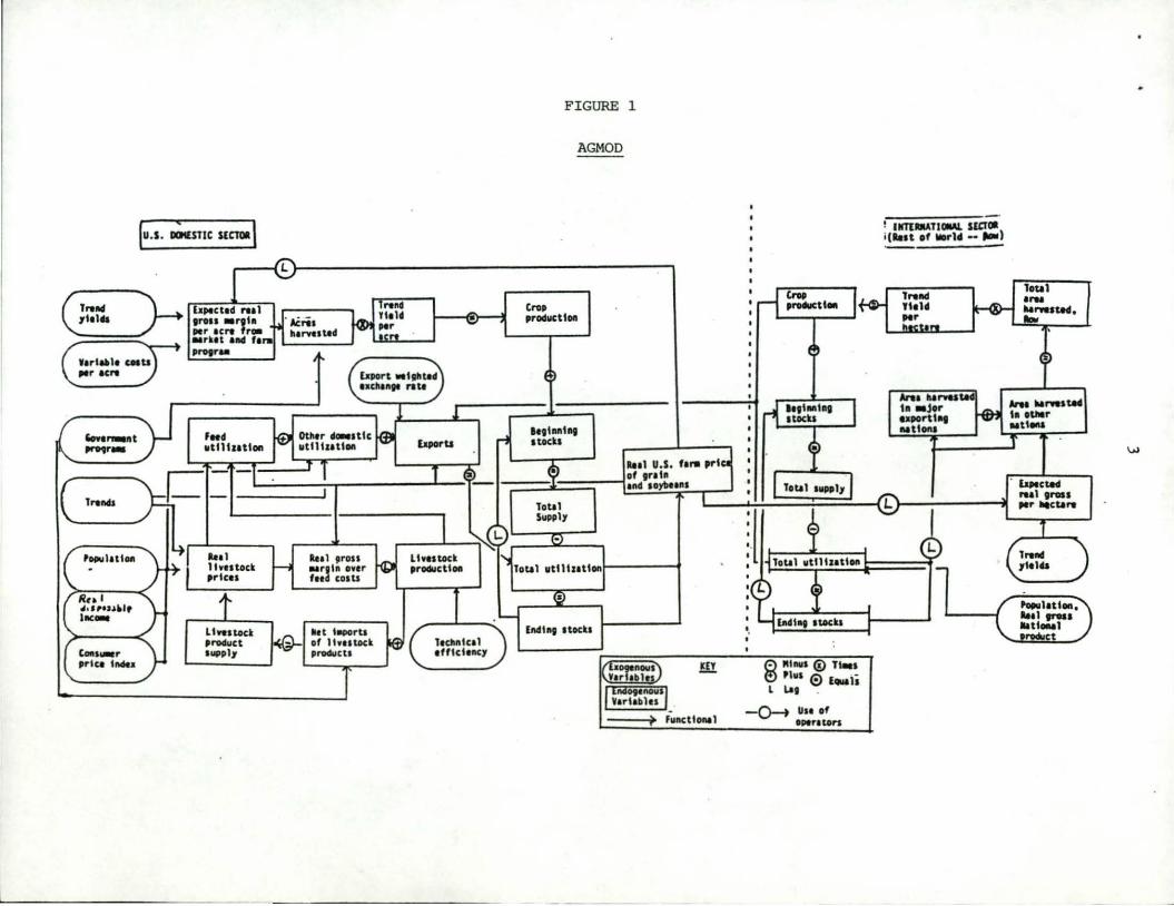
The basic structure of the model is presented in Figure 1. It is primarily recursive,

but involves a simultaneous equation · solution focusing on the real U.S. farm price of

grain and soybeans. The supply equations feature gross margins over variable costs on

crops and gross margins over feed costs on livestock. Gross margin type variables

provide indicators of profits from enterprises over time. Because gross margins tend to

display consistency over time or change in a consistent manner, they provide a means for

diagnostic checking of the forecast. Major departures from past levels or trends are

cause for re-evaluation.

---t ,,..,_

T,.fldl

~.s. ~1c smoa l

bpected nal '""' ·1·· ... , ., ... ,.. .. ,kit .... ,.,.. ,,..., ..

fffd 11ttlh1tton

... 1 lhtstoct ,,., .. lhHlod •r'Oduct 1-.pl1

[Jlp0rt .. tpud udla11tt nu

Otlltr "-•tic utt 1t 11 tton

... 1 , , ... NrJ'" over ftt COIU

lltt l11POrU of lhutoct procklcu

Unnock ,,..,,u ..

Ttdl11tc11 tfflclt11C1

FIGURE 1

A GM OD

••1h111t .. ltOCU

• I

'· •

0 t1t11111 © Tt•s e> Plus 0 l f l ... , . .....

- ()-+ UH of •Ptrators

Ana Ilana t• •Jtr UllClrtl .. MUOlll

lotal ..... ... ,,..led. ...

bpected rul 1n111 ,., lleeure

Trelld ytalu

'°"'lit tc111, ... 1 ,,.... .. tt-1

"*

4

The general format of AGMOD is similar to the MSU Agriculture Model, but with

much less detail, especially in the international sector J./ The international sector is

basically the "rest of the world" except that supply relationships on coarse grain and

wheat are separately derived for the major exporting nations. Also, the availability of

soybeans and soybean meal from Argentina and Brazil was estimated from a sub model.

With an upper limit of 300 variables in Micro TSP, one must be very selective in

order to develop a reasonably comprehensive model. Consequently, the model has been

kept fairly simple. The development strategy was to produce a working version; that is a

version which could consistently be solved and generate reasonable forecasts. As time

permitted, the components of the model were then refined and tested. This approach

was effective because problems were encountered in obtaining solutions in early forms of

AGMOD, a problem that plagued the MSU Agriculture Model. Having a fairly simple

version aided in finding ways to handle this problem.

The speed of solution of the model aided greatly in model development and

diagnostic checking. AGMOD normally solves in 2-3 minutes on an IBM-AT or Zenith

248-82. The graphics options were also employed frequently for identifying problems.

For each statistical equation which was entered into the model, several alternative

equations were estimated--in some cases as many as 5-10 alternative formulations. The

equation with the strongest logical and statistical properties was then selected for

inclusion. Another test was to observe the estimate of the dependent variable in the

model solution for the historical period and the forecast for the projection period. The

estimated values were compared to the actual over the historical period as one test. The

other test was to check how "reasonable" were the forecasts into the future.

J!The MSU Agriculture Model was developed on a mainframe computer in the mid 1970s to mid 1980s. It includes a comprehensive international sector in addition to the domestic component. Gauss-Seidel is also the solution process (MSU Agriculture Model).

------

5

As the model grew in size, a decision was made to forego the ability to compare

the estimates from the model with the actual. This required two codes for each

variable-actual and estimated. In order to enlarge the model, each variable was given

only one code name which represented actual values over the historical period and

forecast values in the future.

The size of the model is an asset in terms of updating. The U.S. Department of

Agriculture, which is the source of most of the data, revises their estimates for the

current year frequently, often monthly. Even recent years' numbers are subject to fairly

regular change. Updating requires 1-2 hours of time each month.

For the first year into the forecast period, which is 1987 in the current formulation

of the model, decisions have to be made as to whether to use the model forecasts or new

government or trade estimates. As the year proceeds, the government or trade

estimates begin to be given more weight than the model forecasts. By the application of

"add" factors in the EDIT mode, the model forecasts can be adjusted to match the

emerging actual figure.

Use for AGMOD

To date, the main use of AGMOD has been for generating long-range projections.

The model is geared to forecast to the year 2000. This information has been used for

planning and budgeting purposes. The projections have also been used as background

information on outlook presentations.

AGMOD is also capable of policy analysis. The current version employs the

program parameters of the Food Security Act of 1985 and accounts for the

implementation of the Conservation Reserve. Assumptions are made about how these

policy tools would be employed as carryover stocks change over time. Alternative

policies could be tested.

An additional application of AGMOD which is yet to be explored is to make the

model stochastic and gain information on market risk. Micro TSP has random number

,....-------------------------------------~------ · -----

l _____ _

6

generators; one of which returns a uniformly distributed random number in the range of 0

to 1; the other returns a normally distributed random number with variance equal to 1.

A possible application of the normally distributed random number generators would

simulate the departure of crop yields from trends. That factor could be added to the

yield equations and with repeated runs of the model the sensitivity of major variables to

yield fluctuations could be discerned. The problem of cross-correlation between corn,

soybean and wheat yields in the U.S. and abroad would have to be addressed.

The applications of the random number generators might be extended to simulating

errors of the forecasts of the component equations in the model, although this might

become a difficult step to take computationally.

If a smaller version of AGMOD could be developed which would allow the

comparison of the model forecasts with actual values over the forec ast period, errors in

the forecasts could be used in risk analysis. Also, this information could be used in the

development of games for teaching forward pricing (Ferris, 1986).

The simplicity and rapid feedback from the model solution might be capitalized

upon in educational programs. The uses could e xplore alternative assumptions with

audiences and clientele and tailor the analysis to the group or individual vie ws.

Satellite Models

While the AGMOD is limited in size, an array of satellite models could be

developed to interface with the core model. These models depend on the output of the

core model, but do not reciprocate. That is, the satellite models have little o r no impact

on the core model. A number of satellite models are slated for development .

1. U.S. models on vegetables, potatoes, dry beans, sugar and fruit.

2. U.S. farm income and expenses.

3. Retail food prices and consumer expenditures on food.

4. Farm price of land.

5. Demand for capital inputs in agriculture.

6. Model of Michigan agriculture; com modi ties, farm income.

7

The solved values for AGMOD for the forecast period could be stored and then

retrieved into the satellite models. These models would, in turn, be solved using the

AGMOD output as exogenous variables.

Further Developmnent and Testing

AGMOD currently incorporates 275 of the maximum 300 variables available in

Micro TSP. With minor modifications, the number could be reduced to about 250

variables. This would provide some flexibility in developing special versions tailored to

address specific problems. For example, the international sector could be enlarged to

include more regional analysis such as was developed for the MSU Agriculture Model

(Shagam, 1987). Alternatively, more detailed subsector models could be incorporated in

the domestic component drawing from such research as the livestock market analysis by

Merlinda Ingco Ongco, 1987). However, the capacity is not available to do both so that

each would serve somewhat different purposes. For many problems, this may not be a

major handicap.

AGMOD remains in a formative stage in that it has not been critiqued by

commodity outlook specialists or those familiar with the general agriculture picture.

More subjective input is needed at this point. A testing ground will be provided in a

symposium on "Large-Scale Models and Economic Policy Analysis" scheduled as a pre­

AAEA conference for August 1988. Several models in the public sector will focus on a

set of policy decisions and the results will be presented at the symposium.

• • 8

References

Ferris, John. "Understanding the Hog Market and How to Forward Price (Including a Game)." Agricultural Economics Staff Paper No. 87-22, March 1987.

Hall, Robert E. and David M. Lilien. Micro TSP User's Manual, Version 5.0. McGraw-Hill Book Company, New York, NY, 1986.

Ingco, Merlinda. "An Econometric Model of U.S. Livestock and Poultry Sector for Policy Analysis and Long-Term Forecasting: Testing of Parameter Stability and Structural Change." Unpublished Ph.D. Dissertation, Department of Agricultural Economics, Michigan State University, 1987.

MSU Agriculture Model. "Long-Term Forecast of U.S. and World Agriculture." Department of Agricultural Economics, Michigan State University, Spring 1985.

Shagam, Shayle. "An International Agricultural Trade Model With Linkage Capability." Volume I and Volume II. Unpublished M.S. Thesis, Department of Agricultural Economics, Michigan State University, 1987.

Shagam, Shayle. "Using Micro TSP With Mainframe Econometric Models." Computers in Agricultural Marketing. Proceedings of a Workshop sponsored by the North Central Computer Institute, October 13-15, 1986, Des Plaines, IL.