Effective Exploration Strategies for the Construction of Visual Maps

Robert Sim and Gregory DudekCentre for Intelligent Machines, McGill University

3480 University St, Montreal, Quebec, Canada H3A 2A7{dudek,simra}@cim.mcgill.ca

Abstract— We consider the effect of exploration policy inthe context of the autonomous construction of a visual mapof an unknown environment. Like other concurrent map-ping and localization (CML) tasks, odometric uncertaintyposes the problem of introducing distortions into the mapwhich are difficult to correct without costly on-line or post-processing algorithms. Our problem is further compoundedby the implicit nature of the visual map representation,which is designed to accommodate a wide variety of visualphenomena without assuming a particular imaging platform,thereby precluding the inference of scene geometry. Such arepresentation presents a requirement for a relatively densesampling of observations of the environment in order toproduce reliable models. Our goal is to develop an on-line policy for exploring an unknown environment whichminimizes map distortion while maximizing coverage. We donot depend on costly post-hoc expectation maximization ap-proaches to improve the output, but rather employ extendedKalman filter (EKF) methods to localize each observationonce, and rely on the exploration policy to ensure thatsufficient information is available to localize the successiveobservations. We present an experimental analysis of avariety of exploratory policies, in both simulated and realenvironments, and demonstrate that with an effective policyan accurate map can be constructed.

I. I NTRODUCTION

In this paper we consider the problem of automaticallyexploring an environment and constructing a visual map.In particular, we are interested in selecting an explorationstrategy which minimizes map uncertainty on-line. Suchuncertainty is accumulated by errors in odometric sensing,and can grow unbounded over time. Our work differs fromother exploration techniques in that the map representationis implicit in nature; that is, we do not produce a geometricdescription of the environment but rather a mapping fromimage features to robot pose. As such, it precludes explicitgeometric inference of landmark positions and henceis not immediately suited to standard Kalman filter, orexpectation maximization techniques [1], [2], [3]. Rather,our goal is to minimize error by selecting an appropriateexploration trajectory which allows the robot to localizeagainst its known map as accurately as possible priorto adding a new observation to the map. We examine avariety of such trajectories, both in simulation and usinga real robot, and present experimental results.

Our approach is aimed at using a purely on-line ex-ploration paradigm to produce a map that is suitable forrobotic navigation. Of course, in many contexts it mightbe desirable to post-process such a map to further optimizeits accuracy, but the current work is motivated by thesupposition that even in such cases a good initial mapis helpful.

A key component of our work is the visual maprepresentation [4]. Unlike the vast majority of mappingparadigms, which employ range sensors derived fromsonar, laser or stereo cameras, visual maps make noattempt to infer scene geometry, but rather encode vi-sual landmarks implicitly in the image domain. As such,visual maps do not require camera calibration, and canencode a wide variety of visual phenomena, includingexotic phenomena such as specularity, shadowing andatmospheric hazing, using arbitrary imaging geometry.The challenge posed by such a representation is that unlikegeometric landmarks it involves no explicit parameters toestimate, and hence is not well-suited to filters which aimto compute maximum-likelihood parameterizations. Thisposes an interesting challenge for autonomous mapping–how to maximize the map likelihood without an explicitrepresentation. It should also be noted that, by definition,an implicit representation makes no prior assumptionsabout imaging geometry, so a further challenge is to inferthe correct map without effectively linearizing away thenonlinear interactive properties of the environment andsensor. Finally, an implicit representation also poses therequirement for a relatively dense sampling of observa-tions covering the pose space. This presents additionalchallenges in that the exploratory trajectory can be quitelong, even in a small environment.

With these challenges in mind, our goal is to developa technique for maximizing coverage of a relatively smallpose space in order to generate an accurate visual map.The mapping process can be made more robust by com-posing a large map using a set of smaller sub-maps [5],[6], [7], [8]. These principles should be applicable to themapping context described here, but can be viewed as asecondary stage of processing and control.

In the following sections we examine previous work

on the CML problem, followed by a description of thevisual mapping framework. We then go on to establish aframework for exploration and discuss several candidateexploration policies. Finally, we present experimental re-sults based on both simulation and validation in our lab,and discuss their implications.

II. RELATED WORK

The problem of concurrent mapping and localization(CML), also known as simultaneous localization and map-ping (SLAM) has received considerable attention in therobotics community [9], [10], [3], [11], [12]. The state ofthe art in CML can be broadly subdivided into one of twoapproaches (and various hybrids). One family of methodscollects measurements and incrementally builds the mapwhile the robot moves (i.e. in an on-line fashion). Usuallythe map is represented as a set of landmarks derived from arange sensor, and a Kalman filter is employed to minimizethe total uncertainty of the robot pose and the individuallandmark positions [1], [2]. These techniques differ fromprevious Kalman filters employed for localization ([9],[10]) in that the landmark positions, as well as the robotpose, are being estimated. While there exist approximationtechniques for reducing the computational expense of on-line CML (c.f. [13]), each update in the standard on-lineapproach is quadratic in the number of landmarks.

The second family of methods for CML involves firstcollecting measurements and then post-processing them ina batch. The standard post-processing method is to employExpectation Maximization (EM), again to minimize the to-tal uncertainty of robot poses and landmark positions [3].One goal of our work is to develop an on-line explorationmethod which maximizes the accuracy of the map withoutresort to expensive map updating. While outside the scopeof this paper, this result can in turn be employed as areliable prior for subsequent EM-style post-processing.

While most of the prior work on mobile robot mappingexploits the use of range data to construct an explicitgeometric map, several authors have considered the use ofvisual data. Nayar,et al were among the first to considerthe use of a purely appearance-based representation of theworld for robot navigation using principal componentsanalysis (PCA) [14]. Pourraz and Crowley consideredthe stability of PCA-based methods for appearance-basednavigation of a mobile robot [15] and Jugessur and Dudeklooked at voting-based methods to make PCA methodsrobust to changes in the scene or illumination [16]. Severalauthors have also considered the use of vision-basedsensing to extract a geometric map, which can then beused in a more traditional CML context. Se,et al extractstereo-based landmarks using a scale-invariant filter [17],and Davison and Kita considered the problem of activelyservoing a stereo head for landmark acquisition as a robottraverses uneven terrain [18]. Finally, Dellaertet al take

advantage of environmental invariants, such as a planarceiling, to construct a mosaic-like map by registering anensemble of images [19].

III. V ISUAL MAPS

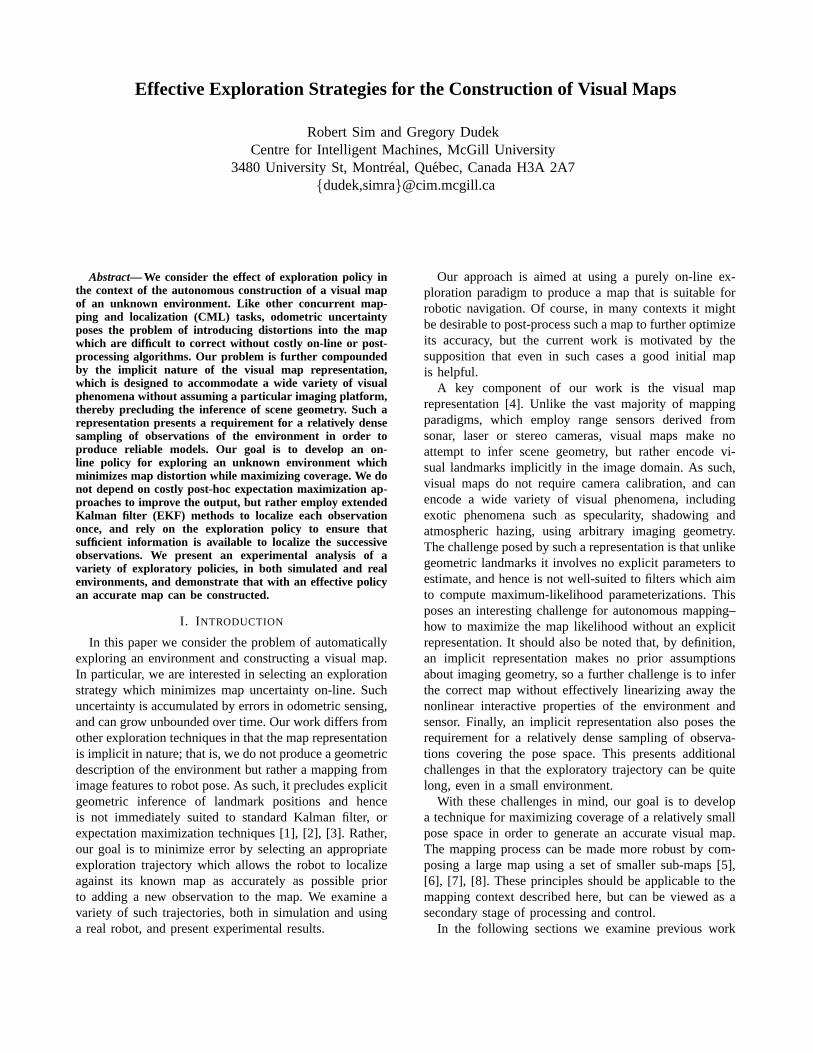
Fig. 1. Landmark Learning Framework: Salient features are detected inthe input images and tracked across the ensemble. The resulting featuresets are subsequently parameterized as functions of the robot pose.

Our visual map representation employs the landmarklearning framework described by Sim and Dudek [4]. Wereview it here in brief and refer the reader to the citedwork for further details.

The key idea is to learn a set of visual features of ascene, and parametrically describe them so that they canbe used to estimate one’s position (that is, they can beused for localization). The features are pre-screened usingan attention operator that efficiently detects statisticallyanomalous parts of an image and robust, useful featuresare tracked over an image ensemble and recorded alongwith an estimate of their individual utility.

The framework operates as follows. Assume for themoment that we have collected an set of observations ofa scene with ground-truth position information associatedwith each image. The landmark learning framework op-erates by first selecting a set of local features from theimages using a measure of visual attention, tracking thosefeatures across the ensemble of images by maximizing thecorrelation of the local image intensity of the feature, andsubsequently parameterizing the set of observed featuresin terms of their behaviour as a function of the knownpositions of the robot (Figure 1). In the context of map-ping, as each image arrives, matches to the parameterizedfeatures are located in the image, the image is localizedfrom the matches using a Kalman Filter (see below), andthe matched observations are inserted into the map usingthe filter estimate as the observation pose.

The feature paramterization employed in [4] computesa radial basis network interpolator of feature propertiessuch as local appearance and image position. In practice,an arbitrary interpolation scheme can be employed and in

this work, for reasons of efficiency, we approximate theinterpolant using bilinear interpolation over the Delaunaytriangulation of the observation poses. Furthermore, againfor efficiency reasons we measure only the image positionof the landmark. Our previous work indicates that whilethe local appearance distribution is informative for local-ization, image position is a stronger and more compactindicator of pose [20].

IV. EXPLORATION FRAMEWORK

We have adapted the Extended Kalman Filter (EKF)localization framework described in the seminal papersby Smith et al and Leonard and Durrant-Whyte as thebasis for our exploration framework [9], [10]. Whilethe work by Leonardet al employed geometric beaconsderived from range sensors as landmarks, the visual maprepresentation instead employs landmark observations inthe visual domain. It should be noted that, unlike EKFimplementations deployed for CML which encode bothrobot pose and landmark position parameters, the onlyparameters maintained in our implementation are thoseof the robot pose. Given that the EKF has been studiedextensively, we repeat here only those aspects of ourimplementation that are particular to our work.

At each time stepk, the robot executes an actionu(k),and takes a subsequent observationz. The plant modelis updated fromu according to the standard EKF formu-lation, and a set of matches to known landmarkszi areextracted from the observed image. Given that the visualmap assumes a 2D configuration space, (that is, fixedorientation) some rehearsal procedure may be requiredto align the camera prior to taking an observation– weconsider this issue in further detail in presenting ourexperimental results.

For each successfully matched landmark, a predictedobservationzi is generated using the visual map, and theinnovationvi(k+1) is computed

vi(k+1) = zi(k+1)− zi(k+1) (1)

The innovation covariance requires estimation of theJacobian of the predicted observation given the map andthe plant estimate. We approximate this Jacobian as thegradient of the nearest face of the model triangulation anddefine it as∇hi . Defined as such, the innovation covariancefollows the standard observation model:

Si(k+1) = ∇hiP(k+1|k)∇hTi +Ri(k+1) (2)

where P is the pose covariance following the actionu,and R is the cross-validation covariance associated withthe learned landmark model. It is important to note thatRserves several purposes– it is simultaneously an overallindicator of the quality of the interpolation model, aswell as the reliability of the matching phase that ledto the observations that define the model; finally it alsoaccomodates the stochastic nature of the sensor.

A. Outlier Detection

It should be noted that feature correspondence takesplace once an observation is obtained. However, theremay be outlier matches that must be filtered out. Assuch, we employ the gating procedure described in [10],with the additional constraint that the gating paramtergis computed adaptively. Specifically, we accept landmarkobservations that meet the constraint

vi(k+1)S−1i (k+1)vT

i (k+1)≤ g2 (3)

whereg = max(gbase, g+2σg) (4)

andgbase is a user defined threshold, and ¯g andσg are theaverage and standard deviation of the set of gating valuescomputed for each landmark observation (that is, the left-hand side of Equation 3). This selection ofg allows thefilter to correct itself when several observations indicatestrong divergence from the predicted observations– indi-cating a high probability that the filter has diverged andaffording the opportunity to correct the error.

B. Map Update

Given the set of gated observations, the EKF is updatedaccording to the standard formulation, whereby the setof filtered innovation measurements is compounded intoa single observation vector and a least-squares solutionis computed for the Kalman gain. Combined with theplant model, a pose estimate and associated covarianceare obtained. Once an updated pose estimate is available,the successfully matched landmarks are inserted into thevisual map, using the estimated pose as their observationpose. It should be noted that we also insert those obser-vations that were removed by the gating procedure. Wetake this approach because it serves to increase the cross-validation covariance associated with the mis-matchedlandmark, thereby reducing its influence for future local-ization. As such, at the end of the exploration procedure,only those landmarks that serve to match reliablyandlocalize reliably can be selected and retained.

In the subsequent section we consider the problem ofselecting exploration trajectories that result in an accuratemap using the EKF framework.

V. EXPLORATION POLICIES

We are interested in comparing candidate robot explo-ration policies with the goal of balancing two competinginterests: coverage and accuracy. In other words, we wantto build the largest, most accurate map possible in a finiteamount of time. Given that there are an infinite number ofpossible exploration trajectories, we will restrict our con-sideration to a set of policies which are either intuitivelysatisfying or serve to illustrate an extreme case. The par-ticular policies we will examine are described below. They

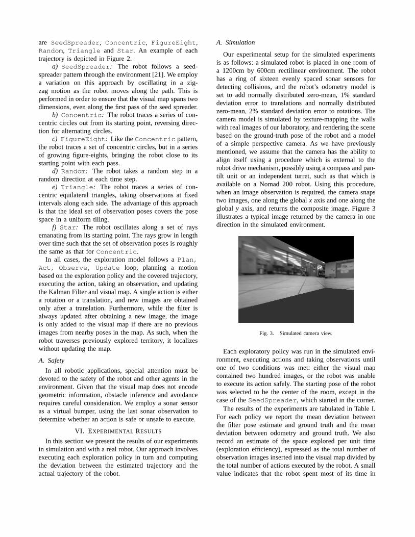
are SeedSpreader , Concentric , FigureEight ,Random, Triangle and Star . An example of eachtrajectory is depicted in Figure 2.

a) SeedSpreader : The robot follows a seed-spreader pattern through the environment [21]. We employa variation on this approach by oscillating in a zig-zag motion as the robot moves along the path. This isperformed in order to ensure that the visual map spans twodimensions, even along the first pass of the seed spreader.

b) Concentric : The robot traces a series of con-centric circles out from its starting point, reversing direc-tion for alternating circles.

c) FigureEight : Like theConcentric pattern,the robot traces a set of concentric circles, but in a seriesof growing figure-eights, bringing the robot close to itsstarting point with each pass.

d) Random: The robot takes a random step in arandom direction at each time step.

e) Triangle : The robot traces a series of con-centric equilateral triangles, taking observations at fixedintervals along each side. The advantage of this approachis that the ideal set of observation poses covers the posespace in a uniform tiling.

f) Star : The robot oscillates along a set of raysemanating from its starting point. The rays grow in lengthover time such that the set of observation poses is roughlythe same as that forConcentric .

In all cases, the exploration model follows aPlan,Act, Observe, Update loop, planning a motionbased on the exploration policy and the covered trajectory,executing the action, taking an observation, and updatingthe Kalman Filter and visual map. A single action is eithera rotation or a translation, and new images are obtainedonly after a translation. Furthermore, while the filter isalways updated after obtaining a new image, the imageis only added to the visual map if there are no previousimages from nearby poses in the map. As such, when therobot traverses previously explored territory, it localizeswithout updating the map.

A. Safety

In all robotic applications, special attention must bedevoted to the safety of the robot and other agents in theenvironment. Given that the visual map does not encodegeometric information, obstacle inference and avoidancerequires careful consideration. We employ a sonar sensoras a virtual bumper, using the last sonar observation todetermine whether an action is safe or unsafe to execute.

VI. EXPERIMENTAL RESULTS

In this section we present the results of our experimentsin simulation and with a real robot. Our approach involvesexecuting each exploration policy in turn and computingthe deviation between the estimated trajectory and theactual trajectory of the robot.

A. Simulation

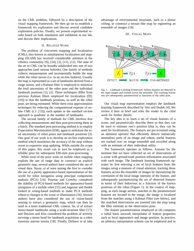
Our experimental setup for the simulated experimentsis as follows: a simulated robot is placed in one room ofa 1200cm by 600cm rectilinear environment. The robothas a ring of sixteen evenly spaced sonar sensors fordetecting collisions, and the robot’s odometry model isset to add normally distributed zero-mean, 1% standarddeviation error to translations and normally distributedzero-mean, 2% standard deviation error to rotations. Thecamera model is simulated by texture-mapping the wallswith real images of our laboratory, and rendering the scenebased on the ground-truth pose of the robot and a modelof a simple perspective camera. As we have previouslymentioned, we assume that the camera has the ability toalign itself using a procedure which is external to therobot drive mechanism, possibly using a compass and pan-tilt unit or an independent turret, such as that which isavailable on a Nomad 200 robot. Using this procedure,when an image observation is required, the camera snapstwo images, one along the globalx axis and one along theglobal y axis, and returns the composite image. Figure 3illustrates a typical image returned by the camera in onedirection in the simulated environment.

Fig. 3. Simulated camera view.

Each exploratory policy was run in the simulated envi-ronment, executing actions and taking observations untilone of two conditions was met: either the visual mapcontained two hundred images, or the robot was unableto execute its action safely. The starting pose of the robotwas selected to be the center of the room, except in thecase of theSeedSpreader , which started in the corner.

The results of the experiments are tabulated in Table I.For each policy we report the mean deviation betweenthe filter pose estimate and ground truth and the meandeviation between odometry and ground truth. We alsorecord an estimate of the space explored per unit time(exploration efficiency), expressed as the total number ofobservation images inserted into the visual map divided bythe total number of actions executed by the robot. A smallvalue indicates that the robot spent most of its time in

−100 −50 0 50 100 150 200 2500

50

100

150

200

250

300

Example Trajectory for iros simul seed3

X position (cm)

Y p

ositi

on (c

m)

(a) SeedSpreader

−200 −150 −100 −50 0 50 100 150

−100

−50

0

50

100

150

Example Trajectory for iros simul concentric

X position (cm)

Y p

ositi

on (c

m)

(b) Concentric

−250 −200 −150 −100 −50 0 50 100 150 200 250−200

−150

−100

−50

0

50

100

150

200

Example Trajectory for iros simul figure eight

X position (cm)

Y p

ositi

on (c

m)

(c) FigureEight

−50 0 50 100 150 200 250 300

−250

−200

−150

−100

−50

0

Example Trajectory for iros simul random

X position (cm)

Y p

ositi

on (c

m)

(d) Random

−150 −100 −50 0 50 100 150

−50

0

50

100

150

Example Trajectory for iros simul triangle

X position (cm)

Y p

ositi

on (c

m)

(e) Triangle

−100 −50 0 50 100 150

−100

−50

0

50

100

Example Trajectory for iros simul star

X position (cm)

Y p

ositi

on (c

m)

(f) Star

Fig. 2. Example Trajectories by Policy

TABLE I

SUMMARY OF EXPLORATION RESULTS BY EXPLORATION POLICY.

Method

MeanFilterError(cm)

MeanOdometricError(cm)

ExplorationEfficiency(images/step)

MaximalDistancefrom O(cm)

SeedSpreader 26.4 43.7 0.178 373Concentric 9.57 4.95 0.496 183FigureEight 5.09 6.87 0.411 242.9Random 8.46 93.4 0.475 347Triangle 30.1 12.0 0.480 173Star 1.63 23.8 <0.001 152

previously explored space. Finally, we report the maximaldistance achieved from the robot’s starting pose.

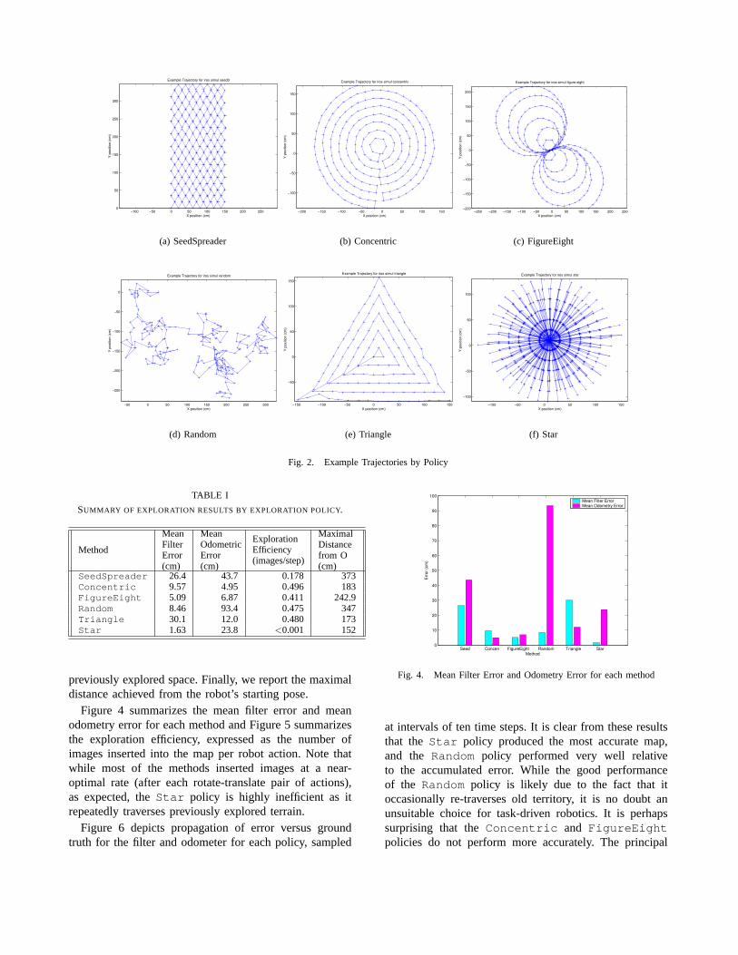
Figure 4 summarizes the mean filter error and meanodometry error for each method and Figure 5 summarizesthe exploration efficiency, expressed as the number ofimages inserted into the map per robot action. Note thatwhile most of the methods inserted images at a near-optimal rate (after each rotate-translate pair of actions),as expected, theStar policy is highly inefficient as itrepeatedly traverses previously explored terrain.

Figure 6 depicts propagation of error versus groundtruth for the filter and odometer for each policy, sampled

Seed Concen FigureEight Random Triangle Star0

10

20

30

40

50

60

70

80

90

100

Method

Err

or (c

m)

Mean Filter ErrorMean Odometry Error

Fig. 4. Mean Filter Error and Odometry Error for each method

at intervals of ten time steps. It is clear from these resultsthat theStar policy produced the most accurate map,and the Random policy performed very well relativeto the accumulated error. While the good performanceof the Random policy is likely due to the fact that itoccasionally re-traverses old territory, it is no doubt anunsuitable choice for task-driven robotics. It is perhapssurprising that theConcentric and FigureEightpolicies do not perform more accurately. The principal

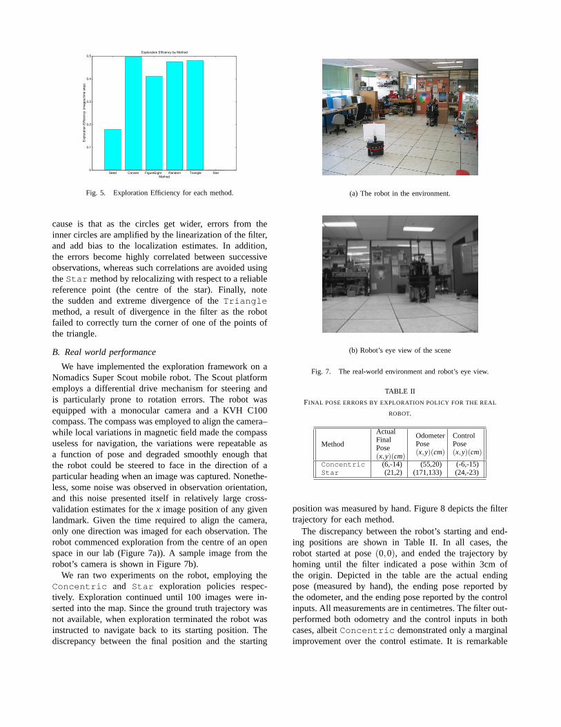
Seed Concen FigureEight Random Triangle Star0

0.1

0.2

0.3

0.4

0.5

Method

Exp

lora

tion

Effi

cien

cy (i

mag

es/ti

me

step

)

Exploration Efficency by Method

Fig. 5. Exploration Efficiency for each method.

cause is that as the circles get wider, errors from theinner circles are amplified by the linearization of the filter,and add bias to the localization estimates. In addition,the errors become highly correlated between successiveobservations, whereas such correlations are avoided usingtheStar method by relocalizing with respect to a reliablereference point (the centre of the star). Finally, notethe sudden and extreme divergence of theTrianglemethod, a result of divergence in the filter as the robotfailed to correctly turn the corner of one of the points ofthe triangle.

B. Real world performance

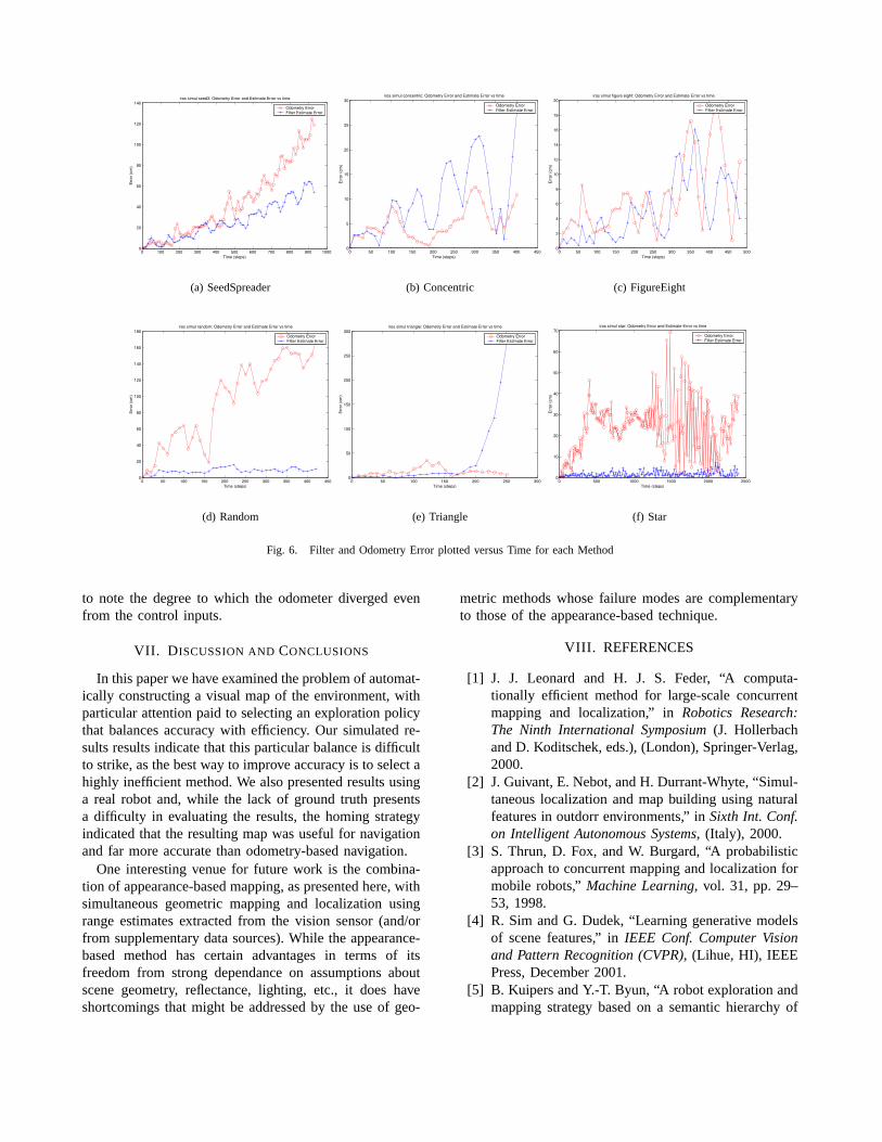
We have implemented the exploration framework on aNomadics Super Scout mobile robot. The Scout platformemploys a differential drive mechanism for steering andis particularly prone to rotation errors. The robot wasequipped with a monocular camera and a KVH C100compass. The compass was employed to align the camera–while local variations in magnetic field made the compassuseless for navigation, the variations were repeatable asa function of pose and degraded smoothly enough thatthe robot could be steered to face in the direction of aparticular heading when an image was captured. Nonethe-less, some noise was observed in observation orientation,and this noise presented itself in relatively large cross-validation estimates for thex image position of any givenlandmark. Given the time required to align the camera,only one direction was imaged for each observation. Therobot commenced exploration from the centre of an openspace in our lab (Figure 7a)). A sample image from therobot’s camera is shown in Figure 7b).

We ran two experiments on the robot, employing theConcentric and Star exploration policies respec-tively. Exploration continued until 100 images were in-serted into the map. Since the ground truth trajectory wasnot available, when exploration terminated the robot wasinstructed to navigate back to its starting position. Thediscrepancy between the final position and the starting

(a) The robot in the environment.

(b) Robot’s eye view of the scene

Fig. 7. The real-world environment and robot’s eye view.

TABLE II

FINAL POSE ERRORS BY EXPLORATION POLICY FOR THE REAL

ROBOT.

Method

ActualFinalPose(x,y)(cm)

OdometerPose(x,y)(cm)

ControlPose(x,y)(cm)

Concentric (6,-14) (55,20) (-6,-15)Star (21,2) (171,133) (24,-23)

position was measured by hand. Figure 8 depicts the filtertrajectory for each method.

The discrepancy between the robot’s starting and end-ing positions are shown in Table II. In all cases, therobot started at pose(0,0), and ended the trajectory byhoming until the filter indicated a pose within 3cm ofthe origin. Depicted in the table are the actual endingpose (measured by hand), the ending pose reported bythe odometer, and the ending pose reported by the controlinputs. All measurements are in centimetres. The filter out-performed both odometry and the control inputs in bothcases, albeitConcentric demonstrated only a marginalimprovement over the control estimate. It is remarkable

0 100 200 300 400 500 600 700 800 900 10000

20

40

60

80

100

120

140iros simul seed3: Odometry Error and Estimate Error vs time

Time (steps)

Err

or (c

m)

Odometry ErrorFilter Estimate Error

(a) SeedSpreader

0 50 100 150 200 250 300 350 400 4500

5

10

15

20

25

30iros simul concentric: Odometry Error and Estimate Error vs time

Time (steps)

Err

or (c

m)

Odometry ErrorFilter Estimate Error

(b) Concentric

0 50 100 150 200 250 300 350 400 450 5000

2

4

6

8

10

12

14

16

18

20iros simul figure eight: Odometry Error and Estimate Error vs time

Time (steps)

Err

or (c

m)

Odometry ErrorFilter Estimate Error

(c) FigureEight

0 50 100 150 200 250 300 350 400 4500

20

40

60

80

100

120

140

160

180iros simul random: Odometry Error and Estimate Error vs time

Time (steps)

Err

or (c

m)

Odometry ErrorFilter Estimate Error

(d) Random

0 50 100 150 200 250 3000

50

100

150

200

250

300iros simul triangle: Odometry Error and Estimate Error vs time

Time (steps)

Err

or (c

m)

Odometry ErrorFilter Estimate Error

(e) Triangle

0 500 1000 1500 2000 25000

10

20

30

40

50

60

70iros simul star: Odometry Error and Estimate Error vs time

Time (steps)

Err

or (c

m)

Odometry ErrorFilter Estimate Error

(f) Star

Fig. 6. Filter and Odometry Error plotted versus Time for each Method

to note the degree to which the odometer diverged evenfrom the control inputs.

VII. D ISCUSSION ANDCONCLUSIONS

In this paper we have examined the problem of automat-ically constructing a visual map of the environment, withparticular attention paid to selecting an exploration policythat balances accuracy with efficiency. Our simulated re-sults results indicate that this particular balance is difficultto strike, as the best way to improve accuracy is to select ahighly inefficient method. We also presented results usinga real robot and, while the lack of ground truth presentsa difficulty in evaluating the results, the homing strategyindicated that the resulting map was useful for navigationand far more accurate than odometry-based navigation.

One interesting venue for future work is the combina-tion of appearance-based mapping, as presented here, withsimultaneous geometric mapping and localization usingrange estimates extracted from the vision sensor (and/orfrom supplementary data sources). While the appearance-based method has certain advantages in terms of itsfreedom from strong dependance on assumptions aboutscene geometry, reflectance, lighting, etc., it does haveshortcomings that might be addressed by the use of geo-

metric methods whose failure modes are complementaryto those of the appearance-based technique.

VIII. REFERENCES

[1] J. J. Leonard and H. J. S. Feder, “A computa-tionally efficient method for large-scale concurrentmapping and localization,” inRobotics Research:The Ninth International Symposium(J. Hollerbachand D. Koditschek, eds.), (London), Springer-Verlag,2000.

[2] J. Guivant, E. Nebot, and H. Durrant-Whyte, “Simul-taneous localization and map building using naturalfeatures in outdorr environments,” inSixth Int. Conf.on Intelligent Autonomous Systems, (Italy), 2000.

[3] S. Thrun, D. Fox, and W. Burgard, “A probabilisticapproach to concurrent mapping and localization formobile robots,”Machine Learning, vol. 31, pp. 29–53, 1998.

[4] R. Sim and G. Dudek, “Learning generative modelsof scene features,” inIEEE Conf. Computer Visionand Pattern Recognition (CVPR), (Lihue, HI), IEEEPress, December 2001.

[5] B. Kuipers and Y.-T. Byun, “A robot exploration andmapping strategy based on a semantic hierarchy of

−100 −50 0 50 100

−80

−60

−40

−20

0

20

40

60

80

100

Filter Trajectory for sloth concentric

X position (cm)

Y p

ositi

on (c

m)

(a) Concentric

−80 −60 −40 −20 0 20 40 60 80 100

−60

−40

−20

0

20

40

60

80

Filter Trajectory for sloth star

X position (cm)

Y p

ositi

on (c

m)

(b) Star

Fig. 8. Filter trajectory for each method

spatial representations,”Robotics and AutonomousSystems, vol. 8, pp. 47–63, 1991.

[6] S. Simhon and G. Dudek, “A global topological mapformed by local metric maps,” inIEEE/RSJ Int. Conf.on Intelligent Robotic Systems, (Victoria, Canada),October 1998.

[7] I. Ulrich and I. Nourbakhsh, “Appearance-basedplace recognition for topological localization,” inProc. IEEE Intl. Conf. on Robotics and Automation,pp. 1023–1029, IEEE Press, April 2000.

[8] H. Choset and K. Nagatani, “Topological simulta-neous localization and mapping (slam): toward ex-act localization without explicit localization,”IEEETrans. on Robotics and Automation, vol. 17, April2001.

[9] R. Smith, M. Self, and P. Cheeseman, “Estimatinguncertain spatial relationships in robotics,” inAu-tonomous Robot Vehicles(I. Cox and G. T. Wilfong,eds.), pp. 167–193, Springer-Verlag, 1990.

[10] J. Leonard and H. F. Durrant-Whyte, “Simultaneousmap building and localization for an autonomousmobile robot,” in IEEE Int. Workshop on IntelligentRobots and Systems, (Osaka, Japan), pp. 1442–1447,November 1991.

[11] B. Yamauchi, A. Schultz, and W. Adams, “Mobilerobot exploration and map building with continuouslocalization,” inIEEE Int. Conf. on Robotics and Au-tomation, (Leuven, Belgium), pp. 3715–2720, IEEEPress, May 1998.

[12] H. Blaasvaer, P. Pirjanian, and H. I. Christensen,“Amor: An autonomous mobile robot navigationsystem,” in IEEE Int. Conf. on Systems, Man, andCybernetics, pp. 2266–2271, 1994.

[13] M. Montemerlo, S. Thrun, D. Koller, and B. Weg-breit, “FastSLAM: A factored solution to the si-multaneous localization and mapping problem,” inAAAI National Conference on Artificial Intelligence,(Edmonton, Canada), AAAI, 2002.

[14] S. Nayar, H. Murase, and S. Nene, “Learning, po-sitioning, and tracking visual appearance,” inIEEEConf on Robotics and Automation, (San Diego, CA),pp. 3237–3246, May 1994.

[15] F. Pourraz and J. L. Crowley, “Continuity propertiesof the appearance manifold for mobile robot positionestimation,” in2nd IEEE Workshop on Perception forMobile Agents, (Ft. Collins, CO), IEEE Press, June1999.

[16] G. Dudek and D. Jugessur, “Robust place recognitionusing local appearance based methods,” inIEEEConf on Robotics and Automation, (San Francisco),IEEE Press, April 2000.

[17] S. Se, D. Lowe, and J. Little, “Vision-based mobilerobot localization and mapping using scale-invariantfeatures,” inIEEE Conf on Robotics and Automation,(Seoul, Korea), pp. 2051–2058, May 2001.

[18] A. J. Davison and N. Kita, “Sequential localisa-tion and map-building for real-time computer visionand robotics,”Robotics and Autonomous Systems,vol. 36, no. 4, pp. 171–183, 2001.

[19] F. Dellaert, W. Burgard, D. Fox, and S. Thrun,“Using the condensation algorithm for robust, vision-based mobile robot localization,” inIEEE Conferenceon Computer Vision and Pattern Recognition, IEEEPress, June 1999.

[20] R. Sim and G. Dudek, “Learning and evaluatingvisual features for pose estimation,” inIEEE Int Confon Computer Vision, (Kerkyra, Greece), IEEE Press,sept 1999.

[21] S. Lumelsky, S. Mukhopadhyay, and K. Sun, “Dy-namic path planning in sensor-based terrain acquisi-tion,” IEEE Trans Robotics and Automation, vol. 6,no. 4, pp. 462–472, 1990.