effective production: measuring of the sales effect using
TRANSCRIPT
Ann Oper ResDOI 10.1007/s10479-015-1932-3
Effective production: measuring of the sales effect usingdata envelopment analysis
Chia-Yen Lee1,2 · Andrew L. Johnson3,4
© Springer Science+Business Media New York 2015
Abstract Sales fluctuations lead to variations in the output levels affecting technical effi-ciency measures of operations when units sold are used at an output measure. The presentstudy uses the concept of “effective production” and “effectiveness” to account for the effectof sales on operational performance measurements in a production system. The effectivenessmeasure complements the efficiency measure which does not account for the sales effect.The Malmquist productivity index is used to measure the sales effects characterized as thedifference between the production function associated with efficiency and the sales-truncatedproduction function associated with effectiveness. The proposed profit effectiveness is dis-tinct from profit efficiency in that it accounts for sales. An empirical study of US airlinesdemonstrates the proposed method which describes the strategic position of a firm and aproductivity-change analysis. These results demonstrate the concept of effectiveness andquantifies the effect of using sales as output.
Keywords Data envelopment analysis · Effectiveness measure · Sales effect · Effectiveproduction · Strategic position
B Chia-Yen [email protected]
Andrew L. [email protected]
1 Institute of Manufacturing Information and Systems, National Cheng Kung University,Tainan City 701, Taiwan
2 Research Center for Energy Technology and Strategy, National Cheng Kung University,Tainan City 701, Taiwan
3 Department of Industrial and Systems Engineering, Texas A&M University,College Station, TX 77840, USA
4 Graduate School of Information Science and Technology, Osaka University, Osaka 565-0871, Japan
123
Ann Oper Res
1 Introduction
In productivity and efficiency analysis, given the same input resources, a firm is called efficientif its output levels are higher than other firms. A typical efficiency study does not distinguishbetween poor performance in terms of production and sales (the performance of the salesgroup) when the outputs are units sold or sales (Lee and Johnson 2014). Thus, this researchcontinues the development of an “effectiveness” measure to quantify a sales effect distinctfrom productive efficiency, in particular, for the Malmquist productivity index in panel dataanalysis (Caves et al. 1982).
In the literature there are two common ways to assess effectiveness. First way is to assessorganizational effectiveness with respect to given goals and objectives. Several researchefforts have used data envelopment analysis (DEA)1 explicitly to address the issue of effec-tiveness analysis. Golany (1988) andGolany et al. (1993) propose that effectivenessmeasurescharacterize how well an organization’s performs when attempting to achieve a goal(s) oran objective(s) and argues that inefficiency is associated with waste, and, therefore, cannotbe associated with effective operations. Golany and Tamir (1995) describe trade-offs amongefficiency, effectiveness, and equality. These authors define an efficiency criterion that seeksto achieve “more-for-less,” i.e., achieving resource savings while maintaining output levelsor expanding outputs generated while maintaining input levels. The effectiveness criterionis determined by the distance between observed outputs and a set of desired goals. Finally,the equality criterion measures the degree of fairness in the allocation of resources or thedistribution of outputs among the units that are evaluated. Asmild et al. (2007) state whenmeasuring effectiveness or other behavioral objectives, multipliers in DEA must reflect real-istic values or prices. Overall effectiveness measures the degree to which a single behavioralor organizational goal such as cost minimization has been attained for a given set of marketprices.
The second way to assess the effectiveness is to use a network analysis to illustrate thedecomposition of a production process (Vaz et al. 2010). Fielding et al. (1985) developperformance evaluation approaches for transportation systems. They distinguish betweenthe production process and the consumption process, arguing that output consumption issubstantially different from output production since transportation services cannot be stored.These authors propose various performance indicators, specifically, service effectiveness,which is the ratio of passenger trip miles over vehicle operating miles. However, singlefactor productivity indicators do not represent all factors in the production system (Chen andMcGinnis 2007). Byrnes and Freeman (1999) measure the efficiency and effectiveness inhealth service.Theydescribe the behavioral health service provision as a two-stageproductionprocess. In the first stage, providers assess client functioning and structure a service planwithin the budget limits. Then, the service plan activities yield changes in client functioningin the second stage. High performance in the first stage is termed cost-efficiency, whereashigh performance in the second stage is term cost-effectiveness. Thus, effectiveness refers toachieving a level of outcome for the least cost. Yu and Lin (2008) use network DEA modelsto characterize a consumption process and assess the service effectiveness and technicaleffectiveness.
The literature regarding the demand (or sales) effect in productivity and efficiency analy-sis is limited. Recently, Lee and Johnson (2011, 2012) use network DEA to decomposea production process into capacity design, demand generation, operations components anddemand consumption, and measure the productivity change of each component. They distin-
1 Charnes et al. (1978), Banker et al. (1984) and Talluri et al. (2006).
123
Ann Oper Res
guish the production process from the demand generation/consumption process. The resultsindicate technical regress can be caused by sales fluctuations rather than production capabil-ities. Further the capacity design component generally has a significant effect on long-termproductivity. Lee and Johnson (2014) propose a demand-truncated production function foreffectiveness measure and use stochastic programming technique to handle demand fluctu-ation. However, the focus of their research is on a cross-sectional production function andtherefore only addresses the relationship between efficiency and effectiveness. This paperconsiders the role of an effectiveness measure when price information and panel data areavailable. Thus, we consider profit effectiveness compared to the more classical profit effi-ciency and we investigate the implications and interpretations possible when a Malmquistproductivity decomposition of effective production is performed.
The paper is organized as follows. Section 2 defines a sales-truncated production functionand illustrates the relationship between efficiency and effectiveness. Section 3 proposes ameasure of sales effect by characterizing the gap between the original production function andthe sales-truncated production function. Section 4 proposes that when evaluating operationalperformance, the measure of profits should be estimated while accounting for the effect ofsales, thus effectiveness rather than efficiency is a useful concept. In Sect. 5 productivitychange and industry growth are quantified using the Malmquist productivity index (MPI).In Sect. 6 the US airline industry is investigated to demonstrate the effectiveness measure.Finally, Sect. 7 concludes the paper.
2 Effective production
2.1 Truncated production function
A production function (PF) defines the maximum outputs that an organization or productionsystem can produce given input resources. Let x be a vector of input variable quantifying theinput resources, y be the single-output variable generated from production system, and yPF
represent maximal output level given inputs. A standard production function with a singleoutput is shown in Eq. (1) and satisfies the properties of nonnegativity, weak essentiality,monotonicity, and concavity (Coelli et al. 2005).
yPF = f (x) (1)
Based on Lee and Johnson (2014), effective output is defined as the output product orservice generated by the production system that is consumed. Furthermore, they define thesales-truncated production function as the maximum sales for a product or service that canbe fulfilled given the quantities of the input resources consumed. A firm is achieving effectiveproduction if the effective output level identified by the sales-truncated production function(STPF) is generated.
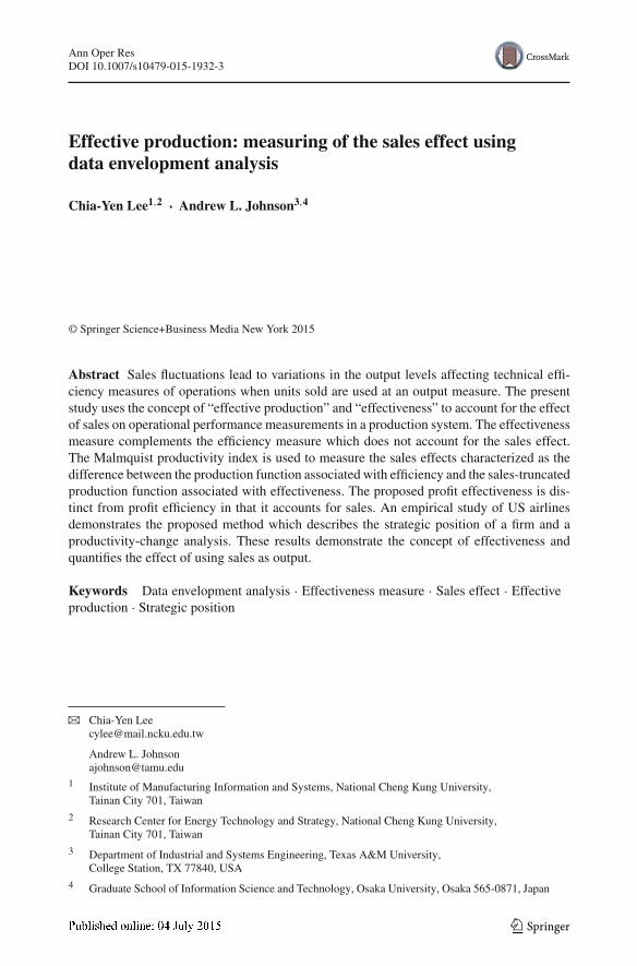
A STPF is defined based on the sales level. To maintain generality, sales are firm-specific,each firm can have a different sales level, and the STPF is defined as the production functiontruncated by the sales of the specific firm. Let s be the realized sales. The effective production,yE , is the smaller of the two variables: the frontier production output level yPF and realizedsales s. The STPF with output level yE is formulated as Eq. (2), where ySTPF is the outputlevel of STPF.
ySTPF = min(yPF , s) = min ( f (x) , s) (2)
123
Ann Oper Res
Y
Fig. 1 Sales-truncated production function
Figure 1 illustrates the STPF and its properties for a single-input and a single-outputcase. For an observation, firm A, the production level is equal to the sales level, SA =Y EA = YA = f (XA). That is, a firm can produce the optimal output level without unfulfilled
sales or excessive inventory. In addition, it is straight-forward to validate the properties-nonnegativity, weak essentiality, monotonicity, and concavity of STPF since the minimumfunction of a production function and constant, sales, is a convex polyhedral.
Now consider amultiple-input andmultiple-output production process. Let x ∈ RI+ denote
a vector of input variables and y ∈ RJ+ denote a vector of output variables for a production
system. The production possibility set (PPS) T is defined as T = {(x, y) : x can produce y}and is estimated by a piece-wise linear convex function enveloping all observations shownin model (3). Let i = {1, 2, . . . , I } be the set of input index, j = {1, 2, . . . , J } be the setof output index, and k = {1, 2, . . . , K } be the set of firm index. Xik is the data of the i thinput resource, Yjk is the amount of the j th production output, and λk is the multiplier forthe kth firm (observation). Model (3) defines the feasible region of the estimated productionpossibility set T̃ . Then, efficiency, θ , can be measured using the variable-returns-to-scale(VRS) DEA estimator which generalizes constant-returns-to-scale (CRS) and captures theeffect of the law of diminishing marginal returns. Output-oriented technical efficiency (T E)
is defined as the distance function Dy(x, y) = inf{θ ∣∣(x, y/θ) ∈ T̃ }.2 If θ = 1, then the firm
is efficient; otherwise it is inefficient when θ < 1.
T̃ ={
(x, y)∣∣∑
kλkYjk ≥ y j ,∀ j;
∑
kλk Xik ≤ xi ,∀i;
∑
kλk = 1; λk ≥ 0,∀k
}
(3)
Similarly, let yE ∈ RJ+ denote an effective output vector produced and consumed. The
sales-truncated production possibility set (PPSE) T E = {(x, yE ) : x can produce yE
that will be consumed in current period} can be estimated by a piece-wise linear convex func-tion truncated by the sales level as shown in (4). Y E
jk is the observation of the amount of thej th output produced by the kth firm and consumed given the firm specific sales S j . That is,Y Ejk = min
(
Yjk, S j)
. The model (4) illustrates the feasible region of the effective production
possibility set T̃ E , where T̃ E is a PPSE estimated by observations with outputs Y Ejk .
2 To avoid the fractional linear programming, the TE is calculated by Dy (x, y) = θ = 1/δ, where δ =sup{δ∣∣ (x, δy) ∈ T̃ }.
123
Ann Oper Res
T̃ E ={
(x, yE )∣∣∑
kλkYjk ≥ yEj ,∀ j; S j ≥ yEj ,∀ j;
∑
kλk Xik
≤ xi ,∀i;∑
kλk = 1; λk ≥ 0,∀k
}
(4)
To complete the discussion we restate a previous result by Lee and Johnson (2014) to char-acterize the STPF.
Proposition 1 The sales-truncated production function (STPF) defined as ySTPF =min( f (x), s) satisfies the underlying properties of nonnegativity, weak essentiality,monotonicity, and concavity.
Proof Recognizing PPSE ⊆ PPS, the underlying properties can be proven directly by usingthe definition ySTPF = min ( f (x), s) and the definition of the properties in Coelli et al.(2005).
2.2 Effectiveness measure
Lee and Johnson (2014) introduced an effectiveness measure with respect to the STPF asfollows.Theoutput-oriented technical effectiveness (TEE ), θ E , is defined as distance function
DEy
(
x, yP) = inf
{
θ E | (x, yP/θ E) ∈ T̃ E
}
where yP is penalized output and defined below.
Assuming producing less than the sales level will lead to lost sales and producingmore outputthan the sales level will lead to inventory holding cost, a generalized effectiveness measureis developed. First, a penalized output Y P
kj is calculated. If Ykj < Skj, then the opportunity to
sell Skj −Ykj units is lost and we set Y Pkj = Ykj −αkj
(
Skj − Ykj) ≥ 0, where αkj
(
Skj − Ykj)
isthe penalty associated with the opportunity cost; otherwise Ykj > Skj and Ykj − Skj units ofinventory are generated and we set Y P
kj = Skj − βkj(
Ykj − Skj) ≥ 0, where βkj
(
Ykj − Skj)
is
the penalty associated with carrying this inventory. In calculating Y Pkj the penalty parameters
αkj ≥ 0 andβkj ≥ 0 are used to quantify the effect of lost sales and inventories, respectively, oneffectiveness. Note this definition of Y P
kj allows for the same normalization of the efficiency
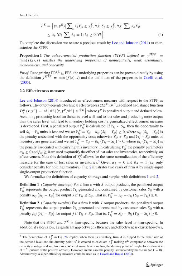
measure for the case of lost sales or inventories.3 Given αA = 0 and βA = 1 (i.e. onlyconsider penalty for holding inventory), Fig. 2 illustrates two cases of firm A by single-inputsingle-output production function.
We formalize the definitions of capacity shortage and surplus with definitions 1 and 2.
Definition 1 (Capacity shortage) For a firm k with J output products, the penalized outputY Pkj represents the output product Ykj generated and consumed by customer sales Skj with a
penalty αkj(
Skj − Ykj)
for output j if Ykj ≤ Skj. That is, Y Pkj = Ykj − αkj
(
Skj − Ykj) ≥ 0.
Definition 2 (Capacity surplus) For a firm k with J output products, the penalized outputY Pkj represents the output product Ykj generated and consumed by customer sales Skj with a
penalty βkj(
Ykj − Skj)
for output j if Ykj > Skj. That is, Y Pkj = Skj − βkj
(
Ykj − Skj) ≥ 0.
Note that the STPF and T E is firm-specific because the sales level is firm-specific. Inaddition, if sales is low, a significant gap between efficiency and effectiveness exists; however,
3 The description of Y PA in Fig. 2b implies when there is inventory, firm A is flipped to the other side of
the demand level and the dummy point A′ is created to calculate Y PA making θ E comparable between the
capacity shortage and surplus cases. When demand levels are low, the dummy point A′ maybe located outsideof T E (outside of the positive orthant). However, in this case the penalty is truncated by the x-axis (or Y = 0).Alternatively, a super efficiency measure could be used as in Lovell and Rouse (2003).
123
Ann Oper Res
(a) (b)
Y
Lost sales
X
Y
Inventory
Penalty
X
Fig. 2 Effectiveness measured by a penalty for capacity shortage, or b penalty for capacity surplus
if sales is high and αkj = 0, efficiency and effectiveness are identical measures. This indicateseffectiveness is particularly important during economic down-turns. Thus, a firm is efficientif θ = 1; otherwise it’s inefficient. Similarly, a firm is effective if θ E = 1 or it’s ineffective.
Proposition 2 (revised from Lee and Johnson 2014:) When sales is large enough, thesales-truncated production possibility set converges to the production possibility set andthe effectiveness converges to efficiency when αkj = 0.
Proof Based on the definition of effectiveness and model (4), for all output j , given αkj = 0,we have Y P
j = Y j and if S j → ∞, then the constraint S j ≥ Y Pj in model (4) is redundant.
Thus, limS j→∞ θ E = θ .
In summary, the definition of sales-truncated production function implies some notableissues. Given this definition, if actual output exceeds sales, then inventories are built and theinventory is ineffective production due to the holding costs and risk of obsolesce of the prod-uct; vice versa, if sales exceeds production, a shortage is created leading to loses in goodwillor market share. Thus, the effectiveness analysis proposed is suitable for characterizing pro-duction systemwith perishable goods,make-to-order production systems, or service systems.
There are two additional considerations in an effectiveness analysis. First, the parametersαkj and βkj characterize the relationship between the opportunity costs and the inventorycosts. In general, we can define αkj as a function of βkj to capture the relationship betweenthese two types of cost.4 Second, the proposed model assumes that output is high enoughthat Y P
kj is not truncated by the x-axis (or Y j = 0) when A′ is constructed.5
2.3 Efficiency v.s. effectiveness
Efficiency and effectiveness complement each other and are not mutually independent, buthave different strategic interpretations (Lee and Johnson 2014). Efficiency measures therelative return on inputs used while effectiveness indicates the ability to match sales given anexisting production technology. High effectiveness generates revenues by providing products
4 For example, let Clkj be the cost of lost sales and Ch
kj be the inventory holding cost of the output j of the
firm k, we can derive the function as αkj = Clkj
Chkj
βkj , ∀k, j . Thus, if βkj = 1, then αkj = Clkj
Chkj.
5 In this case truncation will bias the effectiveness measure and alternative methods based on the superefficiency model alternative would be preferred.
123
Ann Oper Res
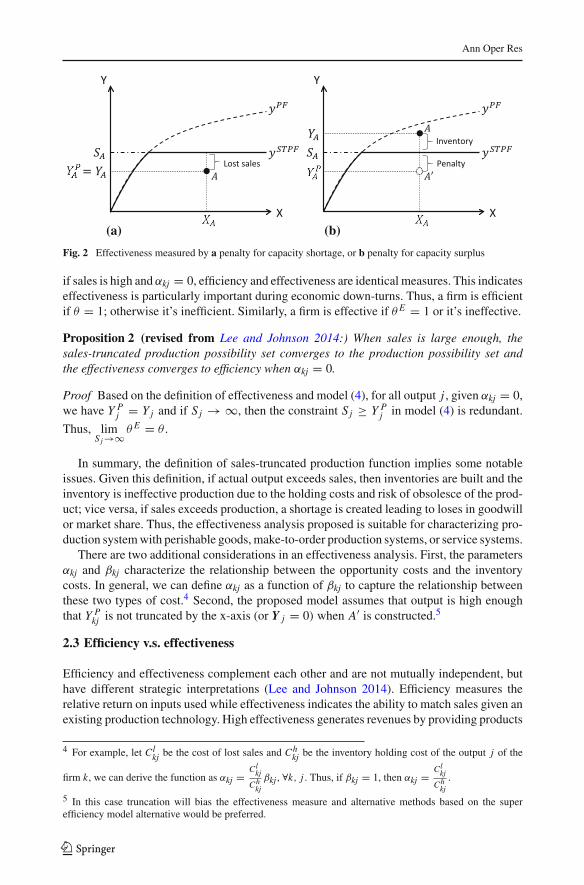
Fig. 3 Strategic position
Low
Effectiveness
Efficiency
Laggard
SalesFocus
ProductionFocus
Leader
High
Low
High
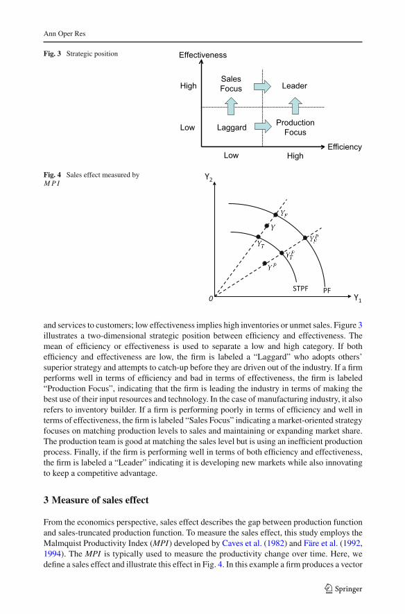
Fig. 4 Sales effect measured byMPI
0PFSTPF
Y1
Y2
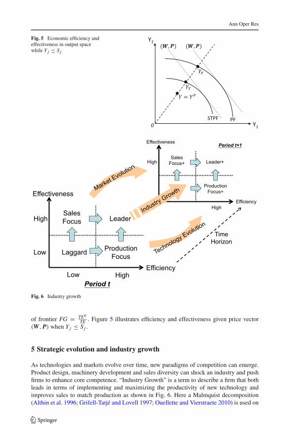
and services to customers; low effectiveness implies high inventories or unmet sales. Figure 3illustrates a two-dimensional strategic position between efficiency and effectiveness. Themean of efficiency or effectiveness is used to separate a low and high category. If bothefficiency and effectiveness are low, the firm is labeled a “Laggard” who adopts others’superior strategy and attempts to catch-up before they are driven out of the industry. If a firmperforms well in terms of efficiency and bad in terms of effectiveness, the firm is labeled“Production Focus”, indicating that the firm is leading the industry in terms of making thebest use of their input resources and technology. In the case of manufacturing industry, it alsorefers to inventory builder. If a firm is performing poorly in terms of efficiency and well interms of effectiveness, the firm is labeled “Sales Focus” indicating a market-oriented strategyfocuses on matching production levels to sales and maintaining or expanding market share.The production team is good at matching the sales level but is using an inefficient productionprocess. Finally, if the firm is performing well in terms of both efficiency and effectiveness,the firm is labeled a “Leader” indicating it is developing new markets while also innovatingto keep a competitive advantage.
3 Measure of sales effect
From the economics perspective, sales effect describes the gap between production functionand sales-truncated production function. To measure the sales effect, this study employs theMalmquist Productivity Index (MPI) developed by Caves et al. (1982) and Färe et al. (1992,1994). The MPI is typically used to measure the productivity change over time. Here, wedefine a sales effect and illustrate this effect in Fig. 4. In this example a firm produces a vector
123
Ann Oper Res
of output Y made up of two types of output, Y1 and Y2. Efficiency is measured relative to aproduction function, PF, and effectiveness is measured relative to a STPF. Output level Yprojected to PF is YF , and projected to STPF is YT (subscript F means “frontier” and Tmeans “truncated frontier”). Similarly the (penalized) effective output vector Y P is projectedto PF and labeled point Y P
F and projected to STPF and labeled point Y PT . The sales effect
is defined using a decomposition of the MPI consisting of the inverse of the effectiveness-
efficiency ratio TEE
TE and the frontier gap (FG).
Sales effect=[
Dy (x, y)
Dy(
x, yP) × DE
y (x, y)
DEy
(
x, yP)
] 12
= Dy (x, y)
DEy
(
x, yP)
[
DEy
(
x, yP)
Dy (x, y)× DE
y (x, y)
Dy(
x, yP)
] 12
=(TEE
TE
)−1
× FG
where
Dy(x, y) = inf{
θ∣∣ (x, y/θ) ∈ T̃
}
= OY/OYF = TE
DEy (x, y) = inf
{
θ E∣∣
(
x, y/θ E)
∈ T̃ E}
= OY/OYT
Dy
(
x, yP)
= inf{
θ∣∣
(
x, yP/θ)
∈ T̃}
= OYP/OYPF
DEy
(
x, yP)
= inf{
θ E∣∣
(
x, yP/θ E)
∈ T̃ E}
= OYP/OYPT = TEE .
Typically MPI is decomposed into the Change in Efficiency (CIE) and Change in (Pro-duction) Technology (CIT). CIE describes the change in technical efficiency while CITcharacterizes the technical change, that is, the shift of the production frontier. TheMPI, CIEand CIT are each interpreted as achieving progress, no change, and regress when the valuesfor their estimates are greater than 1, equal to 1, and less than 1, respectively. Here a parallelstructure for decomposition is used, but the interpretation is adjusted for the current setting.
Sales effect is decomposed into the inverse of the TEE
TE and FG. The effectiveness-efficiency
ratio TEE
TE illustrates the gap between effectiveness and efficiency. If TEE
TE < 1, then the firm
should strive to increase sales and focus on market development. If TEE
TE > 1, then the firmshould focus on productivity to catch upwith the cutting-edge production technology. In addi-tion, the frontier gap (FG) characterizes the sales change, that is, the shift between STPF andPF. STPF is always closer to the origin than PF, thus FGmust be greater-than-or-equal-to 1.
Proposition 3 Based on the decomposition of sales effect, FG is always greater-than-or-
equal-to 1. Thus, if(TEE
TE
)−1> 1, then sales effect must be greater than 1.
Proof Based on footnote 3, output is high enough and Y P should not be less than zero. TheFG can be calculated as follows.
FG =[
DEy
(
x, yP)
Dy (x, y)× DE
y (x, y)
Dy(
x, yP)
] 12
=[
OY P/OY PT
OY/OYF× OY/OYT
OY P/OY PF
] 12
=[
OY PF
OY PT
× OYF
OYT
] 12
≥ 1
123
Ann Oper Res
In particular, STPF cannot move beyond the PF. Thus, sales effect> 1 when(TEE
TE
)−1
> 1.
Sales effect characterizes the frontier gap between STPF and PF. From an economicperspective, sales effect is a measure to account for sales on operational performance. Whileefficiency attributes the entire difference between the production frontier and the observationto operations, the sales effects identifies the part of inefficiency that is attributable to the lackof sales. In particular, given the output price, the revenue efficiency (Nerlove 1965) assumesthat all the output generated from production system can be consumed and may overestimatethe revenue; however, in fact, only sold products generate revenues. In such a case, givenprice information the revenue difference between efficiency and effectiveness results in thesales effect. That is, sales effect characterizes the gap between production revenue (withoutconsidering the sales level) and sales revenue (with considering the sales level) if outputprices are given. We describe economic efficiency in Sect. 4.
4 Economic efficiency and economic effectiveness
Economic efficiency is a measure characterizing the use of resources so as to maximize thevalue of production goods (Coelli et al. 2005). Here we discuss profit efficiency for economic
efficiency. The profit maximization function PF∗ (W,P) = max{{
Py − Wx∣∣ (x,y) ∈ T̃
}}
presents the maximal profit achievable with the given input and output price, where W isa price vector of inputs and P is a price vector of outputs. We define profit efficiency (PE)(Nerlove 1965) as the ratio of the profit of an observation r and the maximum profit given thespecific input and output price PE
(
W,P; xr , yr) = Pyr−Wxr
PF∗(W,P)= PF
PF∗ . Based on the traditionaldefinition of economic efficiency (Farrell 1957), the profit efficiency can be decomposed intoallocative efficiency (AE) and technical efficiency (TE). Specifically, PE = AE× TE, whereTE can be measured by general productivity technique.
As mentioned, only sold products generate revenues. Here a parallel structure similar toeconomic efficiency is used to define economic effectiveness. Economic effectiveness is ameasure characterizing the use of resources so as to maximize the value of sold productsgenerated from a production system. Thus, the profit-maximization function and profit effec-
tiveness is firm-specific and defined as PFE∗r (W,P) = max
{{
PyP − Wx∣∣(
x, yP) ∈ T̃ E
r
}}
and PEEr
(
W,P; xr , yPr) = PyPr −Wxr
PFE∗r (W,P)
= PFEr
PFE∗r
of firm r , where yP is penalized output
related to STPF described in Sect. 2. Similarly, profit effectiveness can be decomposed intoallocative effectiveness (AEE ) and technical effectiveness (TEE ). That is,PEE = AEE×TEE .Note that PE is calculated under the assumption all output can be consumed no matter thesales level; however,PEE considers the effective product with respect to the sales level. Thus,
when sales is limited, the traditional measure of PE is biased. The ratio PEE
PE measures the
gap between economic efficiency and economic effectiveness, and PEE
PE = AEE
AE × TEE
TE .In a special case inwhich all firms under produce, Y j ≤ S j for all j , and the cost associated
with missed sales are negligible, then PEE
PE = PFE/PFE∗PF/PF∗ = PF∗
PFE∗ ≥ 1 because PFE = PF
and T E ⊆ T . This result shows the traditional measure of PE is a lower bound for the trueprofit efficiency (i.e. profit effectiveness) when sales is sufficient.
To address this issue, profit effectiveness is proposed to capture the sales effect. TEE
TEdirectly measures the gap between STPF and PF, a measure of the sales effect on the shift
123
Ann Oper Res
Fig. 5 Economic efficiency andeffectiveness in output spacewhile Y j ≤ S j
0PFSTPF
Y1
Y2
Low
Effectiveness
Efficiency
Laggard
SalesFocus
ProductionFocus
Leader
High
Low
High
Period t
Effectiveness
Efficiency
SalesFocus+
ProductionFocus+
Leader+
High
High
Period t+1
TimeHorizon
Fig. 6 Industry growth
of frontier FG = TEE
TE . Figure 5 illustrates efficiency and effectiveness given price vector(W,P) when Y j ≤ S j .
5 Strategic evolution and industry growth
As technologies and markets evolve over time, new paradigms of competition can emerge.Product design, machinery development and sales diversity can shock an industry and pushfirms to enhance core competence. “Industry Growth” is a term to describe a firm that bothleads in terms of implementing and maximizing the productivity of new technology andimproves sales to match production as shown in Fig. 6. Here a Malmquist decomposition(Althin et al. 1996; Grifell-Tatjé and Lovell 1997; Ouellette and Vierstraete 2010) is used on
123
Ann Oper Res
both efficiency and the new effectiveness measure to measure market evolution, technologyevolution, or identify industry growths using the measure of productivity change with respectto efficiency and effectiveness (all of which are defined rigorously below).
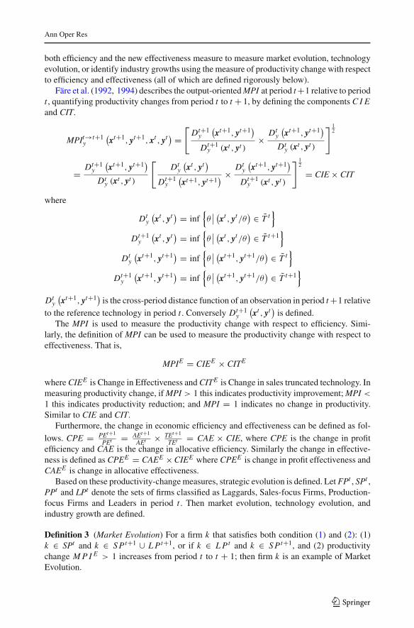
Färe et al. (1992, 1994) describes the output-orientedMPI at period t+1 relative to periodt , quantifying productivity changes from period t to t + 1, by defining the components C I Eand CIT.
MPIt→t+1y
(
xt+1, yt+1, xt , yt) =
[
Dt+1y
(
xt+1, yt+1)
Dt+1y (xt , yt )
× Dty
(
xt+1, yt+1)
Dty (xt , yt )
] 12
= Dt+1y
(
xt+1, yt+1)
Dty (xt , yt )
[
Dty
(
xt , yt)
Dt+1y
(
xt+1, yt+1) × Dt
y
(
xt+1, yt+1)
Dt+1y (xt , yt )
] 12
= CIE × CIT
where
Dty
(
xt , yt) = inf
{
θ∣∣(
xt , yt/θ) ∈ T̃ t
}
Dt+1y
(
xt , yt) = inf
{
θ∣∣(
xt , yt/θ) ∈ T̃ t+1
}
Dty
(
xt+1, yt+1) = inf{
θ∣∣(
xt+1, yt+1/θ) ∈ T̃ t
}
Dt+1y
(
xt+1, yt+1) = inf{
θ∣∣(
xt+1, yt+1/θ) ∈ T̃ t+1
}
Dty
(
xt+1, yt+1)
is the cross-period distance function of an observation in period t+1 relativeto the reference technology in period t . Conversely Dt+1
y
(
xt , yt)
is defined.The MPI is used to measure the productivity change with respect to efficiency. Simi-
larly, the definition of MPI can be used to measure the productivity change with respect toeffectiveness. That is,
MPIE = CIEE × CITE
whereCIEE is Change in Effectiveness andCITE is Change in sales truncated technology. Inmeasuring productivity change, ifMPI > 1 this indicates productivity improvement;MPI <
1 this indicates productivity reduction; and MPI = 1 indicates no change in productivity.Similar to CIE and CIT.
Furthermore, the change in economic efficiency and effectiveness can be defined as fol-
lows. CPE = PEt+1
PEt = AEt+1
AEt × TEt+1
TEt = CAE × CIE, where CPE is the change in profitefficiency and CAE is the change in allocative efficiency. Similarly the change in effective-ness is defined as CPEE = CAEE ×CIEE where CPEE is change in profit effectiveness andCAEE is change in allocative effectiveness.
Based on these productivity-changemeasures, strategic evolution is defined. Let FPt , SPt ,PPt and LPt denote the sets of firms classified as Laggards, Sales-focus Firms, Production-focus Firms and Leaders in period t . Then market evolution, technology evolution, andindustry growth are defined.
Definition 3 (Market Evolution) For a firm k that satisfies both condition (1) and (2): (1)k ∈ SPt and k ∈ SPt+1 ∪ LPt+1, or if k ∈ LPt and k ∈ SPt+1, and (2) productivitychange MPI E > 1 increases from period t to t + 1; then firm k is an example of MarketEvolution.
123
Ann Oper Res
Definition 4 (Technology Evolution) For a firm k that satisfies both condition (1) and (2):(1) k ∈ PPt and k ∈ PPt+1 ∪ LPt+1, or if k ∈ LPt and k ∈ PPt+1, and (2) the productivitychangeMPI > 1 progresses from period t to t + 1; then firm k is an example of TechnologyEvolution.
Definition 5 (Industry Growth) For a firm k that satisfies both condition (1) and (2): (1)k ∈ LPt and k ∈ LPt+1, and (2) the productivity change MPI > 1 or MPIE > 1 progressesfrom period t to t + 1; then firm k is an example of Industry Growth.
We assume the production possibility set expands as improved methods for productionbecome available, thus Diewert’s sequential model (1980, 1992) is used. The reference set toevaluate a production process in a given period is constructed by including observations ofthe production processes from that same period and all previous periods. However, applyingDiewert’s sequential model to the estimation of the STPF does not necessarily result in thesales truncated production possibility set expanding because when sales levels fall the salestruncated production possibility set will contract.
6 US airline industry
6.1 Data description
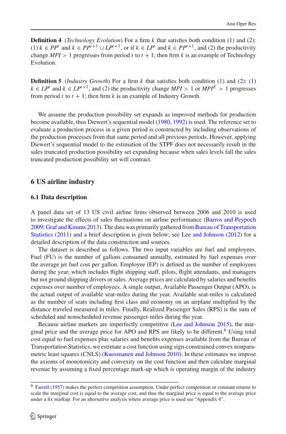
A panel data set of 13 US civil airline firms observed between 2006 and 2010 is usedto investigate the effects of sales fluctuations on airline performance (Barros and Peypoch2009;Graf andKimms2013). The datawas primarily gathered fromBureau of TransportationStatistics (2011) and a brief description is given below; see Lee and Johnson (2012) for adetailed description of the data construction and sources.
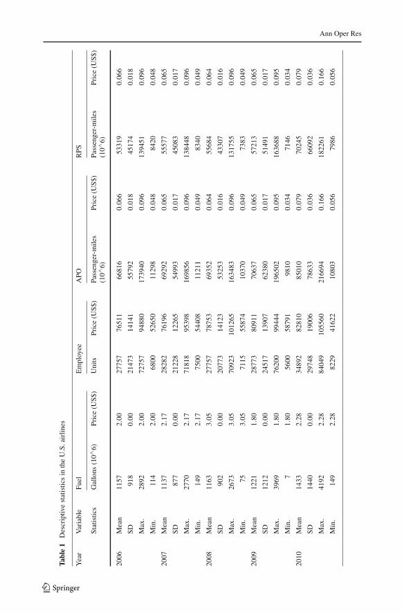
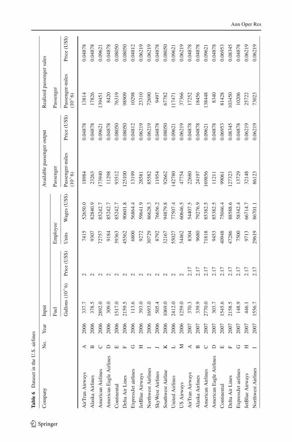
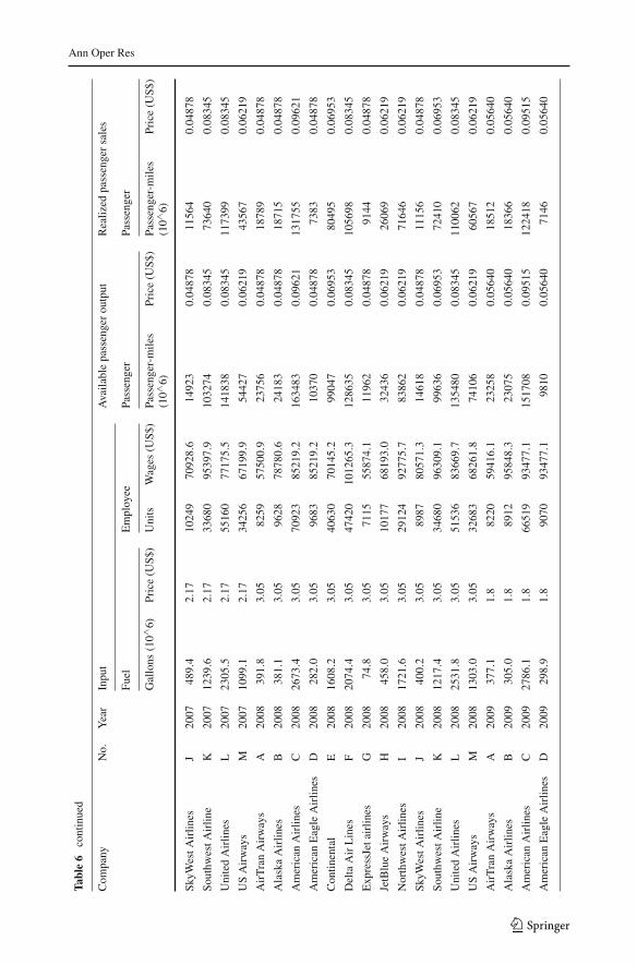
The dataset is described as follows. The two input variables are fuel and employees.Fuel (FU) is the number of gallons consumed annually, estimated by fuel expenses overthe average jet fuel cost per gallon. Employee (EP) is defined as the number of employeesduring the year, which includes flight shipping staff, pilots, flight attendants, and managersbut not ground shipping drivers or sales. Average prices are calculated by salaries and benefitsexpenses over number of employees. A single output, Available Passenger Output (APO), isthe actual output of available seat-miles during the year. Available seat-miles is calculatedas the number of seats including first class and economy on an airplane multiplied by thedistance traveled measured in miles. Finally, Realized Passenger Sales (RPS) is the sum ofscheduled and nonscheduled revenue passenger-miles during the year.
Because airline markets are imperfectly competitive (Lee and Johnson 2015), the mar-ginal price and the average price for APO and RPS are likely to be different.6 Using totalcost equal to fuel expenses plus salaries and benefits expenses available from the Bureau ofTransportation Statistics, we estimate a cost function using sign-constrained convex nonpara-metric least squares (CNLS) (Kuosmanen and Johnson 2010). In these estimates we imposethe axioms of monotonicity and convexity on the cost function and then calculate marginalrevenue by assuming a fixed percentage mark-up which is operating margin of the industry
6 Farrell (1957) makes the perfect competition assumption. Under perfect competition or constant returns toscale the marginal cost is equal to the average cost, and thus the marginal price is equal to the average priceunder a fix markup. For an alternative analysis where average price is used see “Appendix 4”.
123
Ann Oper Res
average 0.0348, see “Appendix 1”.7 Table 1 summarizes the dataset. A further description ofthe data is available in the “Appendix 2”.
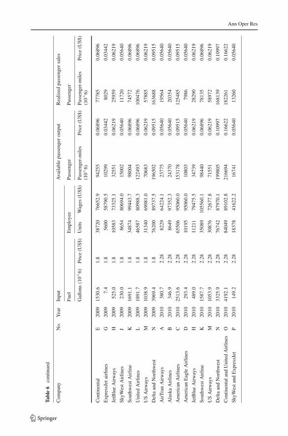
In the panel data, mergers and acquisitions are observed in 2009 and 2010. As reportedin the financial statements, Delta Airlines and Northwest Airlines merged in 2009. Simi-larly, Continental Airlines and United Airlines, and the ExpressJet Airlines and SkyWestAirlines merged in 2010. The effects of merges and acquisitions will be investigated inSect. 6.3.
6.2 Productivity level analysis: strategic position
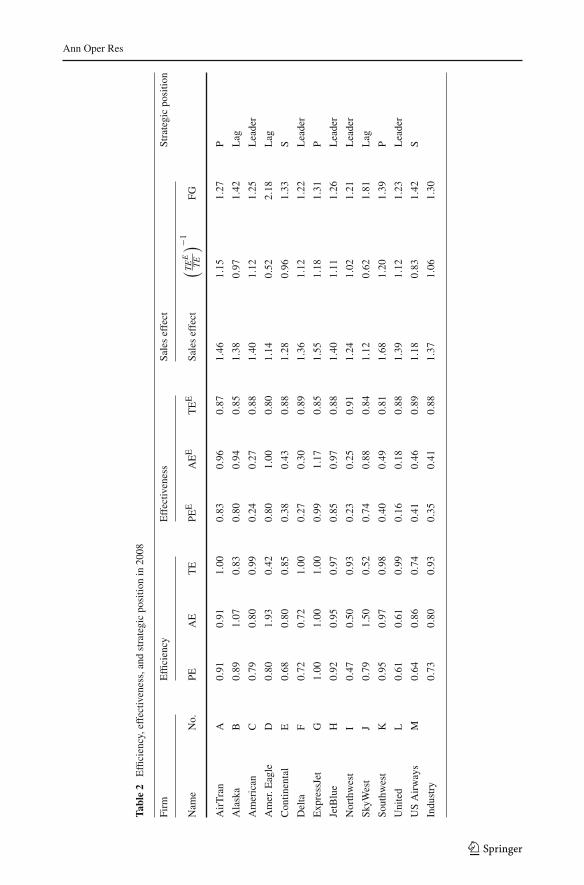
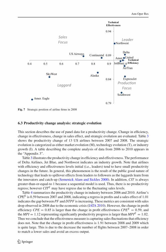
Efficiency, effectiveness, sales effect, and strategic position are estimated.8 In this data setthe actual output is greater than or equal to the sales, i.e., we discuss only the case of capacitysurplus with the penalty parameter βkj = 0.5 since we assume that the cost of two empty seatscan be covered by the payment of one passenger. Table 2 and Fig. 7 show the performance of13 US airline firms in 2008 and the industrial weighted9 average performance. The strategicposition of each airline is categorized as either laggard (Lag), sales focus (S), productionfocus (P), or leader in Fig. 7.
In general all airlines have similarly good levels of technical effectiveness. This indicatesall airlines are effectively matching sales levels to output levels generated. Second, even goodperformance in technical effectiveness, this does not mean firms are generating large profitsbecause most firms have poor profit effectiveness. Take for example Southwest Airlines, ithas an excellent profit efficiency but poor profit effectiveness. In the airline industry, halfof airlines perform poorly in terms of allocative effectiveness, thus given the current saleslevel the airline is not using the cost efficient mix of labor and capital (i.e., fuel in this case).Third, Southwest has a larger sales effect, that is the gap between PF and STPF is large.Generally, larger sales effects imply the lower sales levels, and thus indicate a lower technicaleffectiveness than industrial average. Southwest should focus on better matching their seatsavailable to the seats customers are demanding. Fourth, at the industry level, the averageprofit efficiency is almost 2.06 times as large as the profit effectiveness, PE = 0.73 andPEE = 0.35. This indicates the severity of the bias in estimating profit using the originalproduction function. Finally, a high allocative efficiency does not guarantee a high allocativeeffectiveness, and vice versa. For instance, the American Airlines allocative efficiency is0.80, higher than average, but its allocative effectiveness is 0.27. American Airlines shouldselect their labor to capital ratio based on their actual sales levels rather than their availableseat levels. Similar conclusions hold for profit efficiency and profit effectiveness. Note thatlower AEE measures the resources wasted due to differences between sales and productionlevels. In the case of airlines, sales is lower than production output in 2006–2010 becauseinventorying seats is not possible. Large fixed capital investments limit the airline’s flexibilityto adjust to fluctuating sales, in particular, downturns.
7 Sign-constrained CNLS is a deterministic estimator that for a cost function gives the same estimated costlevels as DEA for observed output levels, but typically has different estimates of marginal cost. Under certainconditions the equivalence between the two estimators is shown in Kuosmanen and Johnson (2010). Thespecific estimator of the cost function used is shown in “Appendix 1”.8 Negative profits can occur. To maintain positive profits for the analysis, a constant dollar value is added toeach airline’s profits. This transformation maintains an ordinal ranking in PE and PEE , however the cardinalrange is condensed. This issue may lead to AE and AEE larger than 1, but does not affect our result andconclusion.9 Passenger-miles is used as weights.
123
Ann Oper Res
Table1
Descriptiv
estatisticsin
theU.S.airlin
es
Year
Variable
Fuel
Employee
APO
RPS
Statistics
Gallons
(10∧
6)Price(U
S$)
Units
Price(U
S$)
Passenger-miles
(10∧
6)Price(U
S$)
Passenger-miles
(10∧
6)Price(U
S$)
2006
Mean
1157
2.00
2775
776
511
6681
60.06
653
319
0.06
6
SD91
80.00
2147
314
141
5579
20.01
845
174
0.01
8
Max.
2892
2.00
7275
794
880
1739
400.09
613
9451
0.09
6
Min.
114
2.00
6800
5265
011
298
0.04
884
200.04
8
2007
Mean
1137
2.17
2828
276
196
6929
20.06
555
577
0.06
5
SD87
70.00
2122
812
265
5499
30.01
745
083
0.01
7
Max.
2770
2.17
7181
895
398
1698
560.09
613
8448
0.09
6
Min.
149
2.17
7500
5440
811
211
0.04
983
400.04
9
2008
Mean
1163
3.05
2775
778
753
6935
20.06
455
684
0.06
4
SD90
20.00
2077
314
123
5325
30.01
643
307
0.01
6
Max.
2673
3.05
7092
310
1265
1634
830.09
613
1755
0.09
6
Min.
753.05
7115
5587
410
370
0.04
973
830.04
9
2009
Mean
1221
1.80
2877
380
911
7063
70.06
557
213
0.06
5
SD12
120.00
2451
713
907
6238
00.01
751
491
0.01
7
Max.
3969
1.80
7620
099
444
1965
020 .09
516
3688
0.09
5
Min.
71.80
5600
5879
198
100.03
471
460.03
4
2010
Mean
1433
2.28
3489
282
810
8501
00.07
970
245
0.07
9
SD14
400.00
2974
819
006
7863
30.03
666
092
0.03
6
Max.
4192
2.28
8404
910
5560
2166
940.16
618
2261
0.16
6
Min.
149
2.28
8229
4162
210
803
0.05
679
860.05
6
123
Ann Oper Res
Table2
Efficiency,effectiv
eness,andstrategicpositio
nin
2008
Firm
Efficiency
Effectiv
eness
Saleseffect
Strategicpositio
n
Nam
eNo.
PEAE
TE
PEE
AEE
TEE
Saleseffect
(TEE
TE
)−1
FG
AirTran
A0.91
0.91
1.00
0.83
0.96
0.87
1.46
1.15
1.27
P
Alaska
B0.89
1.07
0.83
0.80
0.94
0.85
1.38
0.97
1.42
Lag
American
C0.79
0.80
0.99
0.24
0.27
0.88
1.40
1.12
1.25
Leader
Amer.E
agle
D0.80
1.93
0.42
0.80
1.00
0.80
1.14
0.52
2.18
Lag
Con
tinental
E0.68
0.80
0.85
0.38
0.43
0.88
1.28
0.96
1.33
S
Delta
F0.72
0.72
1.00
0.27
0.30
0.89
1.36
1.12
1.22
Leader
ExpressJet
G1.00
1.00
1.00
0.99
1.17
0.85
1.55
1.18
1.31
P
JetBlue
H0.92
0.95
0.97
0.85
0.97
0.88
1.40
1.11
1.26
Leader
Northwest
I0.47
0.50
0.93
0.23
0.25
0.91
1.24
1.02
1.21
Leader
SkyW
est
J0.79
1.50
0.52
0.74
0.88
0.84
1.12
0.62
1.81
Lag
Southw
est
K0.95
0.97
0.98
0.40
0.49
0.81
1.68
1.20
1.39
P
United
L0.61
0.61
0.99
0.16
0.18
0.88
1.39
1.12
1.23
Leader
USAirways
M0.64
0.86
0.74
0.41
0.46
0.89
1.18
0.83
1.42
S
Indu
stry
0.73
0.80
0.93
0.35
0.41
0.88
1.37
1.06
1.30
123
Ann Oper Res
AirTran
Alaska
Amer.
Amer. Eagle
ContinentalDelta
ExpressJet
JetBlue
Northwest
SkyWest
Southwest
UnitedUS Airways
0.79
0.84
0.89
0.94
0.4 0.5 0.6 0.7 0.8 0.9 1.0
TechnicalEffectiveness
TechnicalEfficiency
SalesFocus Leader
Produc�onFocus
Laggard
Fig. 7 Strategic position of airline firms in 2008
6.3 Productivity change analysis: strategic evolution
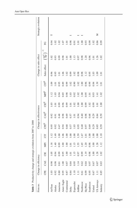
This section describes the use of panel data for a productivity change. Change in efficiency,change in effectiveness, change in sales effect, and strategic evolution are evaluated. Table 3shows the productivity change of 13 US airlines between 2007 and 2008. The strategicevolution is categorized as either market evolution (M), technology evolution (T), or industrygrowth (I). A table describing the complete analysis of data from 2006 to 2010 appears inthe “Appendix 3”.
Table 3 illustrates the productivity change in efficiency and effectiveness. The performanceof Delta Airlines, Jet Blue, and Northwest indicates an industry growth. Note that airlineswith efficiency and effectiveness levels initial (i.e., leaders) tend to have small productivitychanges in the future. In general, this phenomenon is the result of the public good nature oftechnology that leads to spillover effects from leaders to followers as the laggards learn fromthe innovators and catch-up (Semenick Alam and Sickles 2000). In addition, CIT is alwaysgreater-than-or-equal-to 1 because a sequential model is used. Thus, there is no productivityregress; however CITE may have regress due to the fluctuating sales levels.
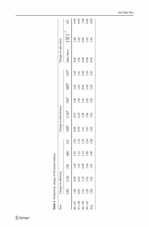
Table 4 summarizes the productivity change in industry between 2006 and 2010. Airline’sCPEE is 0.59 between 2007 and 2008, indicating a regress in profits and a sales effect of 1.01indicates the gap betweenPF andDTPF is increasing. Thesemetrics are consistent with salesdrop observed in 2008 due to the economic crisis (IATA 2010). However, the change in profitefficiency CPE = 0.85 is larger than the change in profit effectiveness CPEE = 0.59, andtheMPI = 1.12 representing significantly productivity progress is larger thanMPIE = 1.02.Thuswe conclude that the effectivenessmeasure is capturing sales fluctuations that efficiencydoes not. Note that the change in profit effectiveness is 1.91 between 2008 and 2009 whichis quite large. This is due to the decrease the number of flights between 2007–2008 in orderto match a lower sales and avoid an excess output.
123
Ann Oper Res
Table3
Prod
uctiv
itychange
andstrategicevolutionfrom
2007
to20
08
Firm
no.
Changein
efficiency
Changein
effectiveness
Changein
saleseffect
Strategicevolution
CPE
CAE
CIE
MPI
CIT
CPE
ECAEE
CIE
EMPI
ECIT
ESaleseffect
(TEE
TE
)−1
FG
AirTran
1.03
0.98
1.05
1.18
1.12
0.95
0.92
1.03
1.12
1.09
0.96
1.02
0.94
T
Alaska
0.92
0.98
0.94
1.40
1.49
0.92
0.91
1.01
1.03
1.01
0.95
0.93
1.02
American
0.80
0.81
0.99
0.99
1.00
0.47
0.48
0.99
0.94
0.95
1.01
0.99
1.02
Amer.E
agle
0.95
1.00
0.95
1.00
1.06
0.94
0.98
0.96
0.85
0.89
1.06
0.98
1.07
Con
tinental
0.87
0.87
1.00
1.00
1.00
0.68
0.69
0.99
0.98
0.99
1.02
1.01
1.01
Delta
0.84
0.84
1.01
1.01
1.00
0.57
0.57
1.01
1.03
1.02
0.99
1.00
0.98
I
ExpressJet
1.10
0.95
1.15
1.15
1.00
1.03
1.01
1.02
0.92
0.90
1.02
1.13
0.91
JetBlue
1.11
1.14
0.97
1.55
1.59
0.95
0 .94
1.00
1.02
1.02
0.98
0.97
1.01
I
Northwest
0.61
0.62
0.99
1.65
1.67
0.40
0.40
1.00
1.00
1.00
0.98
0.98
1.00
I
SkyW
est
0.99
0.84
1.19
1.20
1.01
0.97
0.98
0.99
0.95
0.96
1.12
1.20
0.93
Southw
est
0.95
0.97
0.98
0.98
1.00
0.69
0.68
1.02
1.01
0.99
0.95
0.96
0.99
United
0.67
0.67
1.00
1.00
1.00
0.29
0.29
0.99
0.93
0.94
1.03
1.01
1.02
USAirways
1.11
0.87
1.28
1.28
1.00
0.85
0.84
1.01
1.41
1.39
1.09
1.26
0.86
M
Indu
stry
0.85
0.83
1.02
1.12
1.10
0.59
0.59
1.00
1.02
1.01
1.01
1.02
0.99
123
Ann Oper Res
Table4
Prod
uctiv
itychange
ofUSairlineindu
stry
Year
Changein
efficiency
Changein
effectiveness
Changein
saleseffect
CPE
CAE
CIE
MPI
CIT
CPE
ECAEE
CIE
EMPI
ECIT
ESaleseffect
(TEE
TE
)−1
FG
06->
071.00
0.99
1.00
1.03
1.02
0.98
0.97
1.00
1.05
1.05
0.99
1.00
0.99
07->
080.85
0.83
1.02
1.12
1.10
0.59
0.59
1.00
1.02
1.01
1.01
1.02
0.99
08->
091.23
1.25
0.99
1.15
1.16
1.91
1.89
1.01
0.96
0.96
0.98
0.98
1.00
09->
101.05
1.01
1.04
1.08
1.03
1.07
1.06
1.01
1.04
1.03
0.98
1.02
0.96
Avg
.1.02
1.01
1.01
1.09
1.08
1.04
1.04
1.01
1.02
1.01
0.99
1.01
0.99
123
Ann Oper Res
Table5
Prod
uctiv
itychange
ofthemergersfrom
2008
to20
10
Year
Firm
no.
Changein
efficiency
Changein
effectiveness
Changein
saleseffect
Strategicevolution
CPE
CAE
CIE
MPI
CIT
CPE
ECAEE
CIE
EMPI
ECIT
ESaleseffect
(TEE
TE
)−1
FG
08->
09F-
>N
1.38
1.38
1.00
1.55
1.55
1.90
1.89
1.01
0.94
0.93
0.98
0.99
0.99
I
I->N
2.12
1.99
1.07
1.64
1.53
2.23
2.26
0.98
0.92
0.93
1.08
1.09
0.99
I
Indu
stry
1.23
1.25
0.99
1.15
1.16
1.91
1.89
1.01
0.96
0.96
0.98
0.98
1.00
09->
10N
1.01
1.01
1.00
1.05
1.05
1.21
1.20
1.01
1.03
1.03
0.98
0.99
0.99
I
E->
O1.27
1.05
1.21
1.27
1.05
1.14
1.12
1.01
1.04
1.02
1.06
1.19
0.89
M
L->
O1.14
1.09
1.05
1.12
1.07
1.22
1.20
1.02
1.04
1.02
0.98
1.03
0.95
I
G->
P0.73
0.93
0.79
0.79
1.00
0.85
0.84
1.01
0.68
0.67
0.86
0.78
1.11
J->P
0.91
0.75
1.22
1.22
1.00
0.97
0.96
1.01
0.68
0.67
1.08
1.20
0.89
Indu
stry
1.05
1.01
1.04
1.08
1.03
1.07
1.06
1.01
1.04
1.03
0.98
1.02
0.96
The
notatio
nF-
>Nmeans
thefirm
Fismergedto
thefirm
N
123
Ann Oper Res
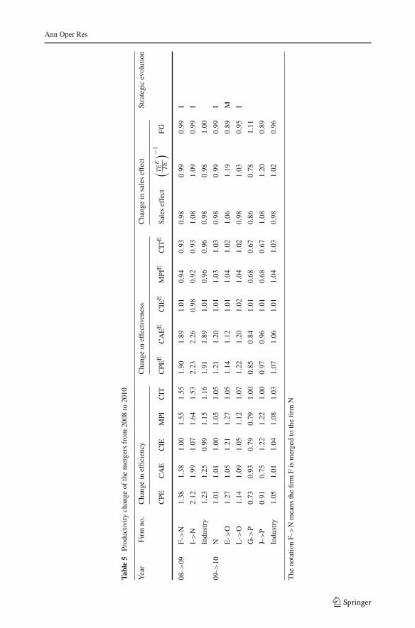
Table 5 illustrates changes in performance due to mergers.10 Let “N” represent the mergedairline consisting of Delta Airlines and Northwest Airlines, “O” represent the merged air-line consisting of Continental Airlines and United Airlines, and “P” represent the mergedairline consisting of ExpressJet and SkyWest Airlines. Mergers benefit the merging airlinesby improving efficiency through increased economies of scale; whereas a merger may notimprove effectiveness immediately (see all MPI E are lower than the industry average).Even worse the merger may lead to trouble in maintaining customer relationships and lead toprofit loses in the short-term. So while mergers allow a larger scale of operations leading tomore output, sales may not be similarly affected, thus the profit effectiveness could drop asin the case of the Sky West/ExpressJet merger. In particular, the Delta merger significantlyimproved the change in profit effectiveness because of the economic downturn in 2008 andgradual recovery in 2010.11
7 Conclusion
This study uses an effectiveness measure to capture the sales effect in productivity analy-sis, in particular, a panel data analysis. It complements efficiency measures. The concepts ofstrategic position and strategic evolution are developed for identifying the competitive advan-tage using the metrics of efficiency and effectiveness. An empirical study of US airlines isconducted to demonstrate the proposed framework. The results show that effectiveness cap-tures sales fluctuations, in particular, the economic crisis in 2008. Furthermore, mergers andacquisitions in the airline industry are evaluated; we conclude that mergers benefit efficiencyby increasing the scale of operations but not necessarily improve effectiveness in the shortrun.
The effectiveness measure can be applied to the different domains, in particular, serviceindustry whose non-storable commodities once generated need to be consumed immediately.Effectiveness also represents the “real” profit we earn from the consumption. In Sect. 4we demonstrated the traditional measure of profit efficiency is a lower bound for the trueprofit efficiency when sales is sufficient. Thus, effectiveness can capture the sales effect andconnect to profits. To extend the study, capacity planning based on an effectivenessmeasure issuggested rather than efficiency measure which captures only the production capability. Thepurpose of capacity planning is to adjust the input resource to control required output. Thus,an objective of maximizing effectiveness is more appropriate than maximizing efficiencyin helping a firm reallocate resource to maximize profits. In addition, this study focuses onsales fluctuation and develops effectiveness measure. To develop a generalized model foreffectiveness with respect to some variable fluctuation, e.g. interest rate fluctuation, mayprovide new insights to different applications.
10 To assess the cross-period effectiveness of the merger in period t + 1, for two firms in period t relative tothe frontier in period t +1, the sales of merger in period t +1 is separated into two parts according to the salesproportions in period t . Vice versa, the sum of sales in period t is used for the merger in period t + 1 relativeto the frontier in period t .11 The progress indicated by CPEE > 1 does not necessarily mean an increase in sales goes up rather thisindicates the airlines is controlling the input resource to match sales levels. The MPIE is mainly an index toshow the sales growth or drop since it characterizes the STPF.
123
Ann Oper Res
Acknowledgments This research was funded by National Science Council (NSC101-2218-E-006-023) andNational Cheng Kung University Research Center for Energy Technology and Strategy (NCKU RCETS),Taiwan.
Appendix 1: Cost function estimation
The sign-constrained convex nonparametric least squares (CNLS) technique is used to esti-mate the cost function andmarginal cost. CNLS can be traced to the seminal work of Hildreth(1954) and was popularized by Kuosmanen (2008) as a powerful tool for describing theaverage behavior of observations. CNLS avoids strong prior assumptions regarding func-tion form while maintaining the standard regularity conditions from microeconomic theoryfor production functions, namely continuity, monotonicity, and concavity. Kuosmanen andJohnson (2010) demonstrated that inefficiency estimated by the sign-constrained CNLS isequivalent to that estimated by DEA. This study imposes the axioms of monotonicity andconvexity on cost function and estimates it by sing-constrained CNLS to obtain marginalcost estimates (Kuosmanen 2012).
Let Ck be the total cost equal to fuel expenses plus salaries and benefits expenses of firmk. εk be the inefficiency term of firm k. Let index h be an alias of index k, αk be the interceptcoefficient, and βkj be the slope coefficient of the j th output of kth firm. In particular, βkj isthe coefficients of the tangent hyperplanes to the piece-wise linear cost frontier which can beinterpreted as the marginal cost of outputs. We obtain the marginal cost estimate βkj of firmk by solving the following sign-constrained CNLS.
min∑
k ε2k
s.t. lnCk = ln(
αk + ∑
j βkjYkj)
+ εk,∀kαk + ∑
j βkjYkj ≥ αh + ∑
j βhjYkj,∀k,∀hβkj ≥ 0,∀ j, k
εk ≥ 0,∀k
(5)
Next, the marginal price for passenger-miles is a fixed mark-up of marginal cost by oper-ating margin of all firms (i.e., the industry average). Operating margin data is available fromAirlinefinancials.com (2014).
Appendix 2: Dataset
See Table 6.
123
Ann Oper Res
Table6
Datasetin
theU.S.airlin
es
Com
pany
No.
Year
Input
Availablepassengeroutput
Realized
passengersales
Fuel
Employee
Passenger
Passenger
Gallons
(10∧
6)Price(U
S$)
Units
Wages
(US$
)Passenger-miles
(10∧
6)Price(U
S$)
Passenger-miles
(10∧
6)Price(U
S$)
AirTranAirways
A20
0633
7.7
274
1552
650.0
1898
40.04
878
1381
40.04
878
AlaskaAirlin
esB
2006
378.5
293
0782
840.9
2326
30.04
878
1782
60.04
878
American
Airlin
esC
2006
2892
.02
7275
785
242.7
1739
400.09
621
1394
510.09
621
American
EagleAirlin
esD
2006
309.0
291
8485
242.7
1129
80.04
878
8420
0.04
878
Con
tinental
E20
0615
17.0
239
363
8524
2.7
9351
20.08
050
7631
90.08
050
DeltaAirLines
F20
0621
59.5
245
562
9060
1.8
1251
000.08
050
9890
90.08
050
Exp
ressJetairlin
esG
2006
113.6
268
0056
864.4
1319
90.04
812
1029
80.04
812
JetBlueAirways
H20
0639
3.0
292
7259
641.9
2858
10.06
219
2331
00.06
219
NorthwestA
irlin
esI
2006
1693
.02
3072
986
628.3
8558
20.06
219
7269
00.06
219
SkyW
estA
irlin
esJ
2006
505.4
287
9276
656.2
1195
40.04
878
9497
0.04
878
Southw
estA
irlin
eK
2006
1069
.02
3216
794
879.8
9266
20.08
050
6778
20.08
050
UnitedAirlin
esL
2006
2412
.02
5502
777
507.4
1427
800.09
621
1174
710.09
621
USAirways
M20
0612
59.0
234
462
6064
6.5
4775
40.06
219
3736
60.06
219
AirTranAirways
A20
0737
0.3
2.17
8304
5440
7.5
2268
00.04
878
1725
20.04
878
AlaskaAirlin
esB
2007
339.9
2.17
9680
7927
6.9
2419
70.04
878
1845
60.04
878
American
Airlin
esC
2007
2770
.02.17
7181
885
382.5
1698
560.09
621
1384
480.09
621
American
EagleAirlin
esD
2007
303.7
2.17
9453
8538
2.5
1121
10.04
878
8340
0.04
878
Con
tinental
E20
0715
45.6
2.17
4094
875
046.4
9906
10.06
953
8142
80.06
953
DeltaAirLines
F20
0721
58.5
2.17
4728
688
588.6
1273
230.08
345
1034
500.08
345
Exp
ressJetairlin
esG
2007
148.9
2.17
7500
5834
2.4
1372
90.04
878
1020
60.04
878
JetBlueAirways
H20
0744
6 .1
2.17
9713
6671
4.7
3214
80.06
219
2572
20.06
219
NorthwestA
irlin
esI
2007
1556
.72.17
2961
986
701.1
8612
30.06
219
7302
30.06
219
123
Ann Oper Res
Table6
continued
Com
pany
No.
Year
Input
Availablepassengeroutput
Realized
passengersales
Fuel
Employee
Passenger
Passenger
Gallons
(10∧
6)Price(U
S$)
Units
Wages
(US$
)Passenger-miles
(10∧
6)Price(U
S$)
Passenger-miles
(10∧
6)Price(U
S$)
SkyW
estA
irlin
esJ
2007
489.4
2.17
1024
970
928.6
1492
30.04
878
1156
40.04
878
Southw
estA
irlin
eK
2007
1239
.62.17
3368
095
397.9
1032
740.08
345
7364
00.08
345
UnitedAirlin
esL
2007
2305
.52.17
5516
077
175.5
1418
380.08
345
1173
990.08
345
USAirways
M20
0710
99.1
2.17
3425
667
199.9
5442
70.06
219
4356
70.06
219
AirTranAirways
A20
0839
1.8
3.05
8259
5750
0.9
2375
60.04
878
1878
90.04
878
AlaskaAirlin
esB
2008
381.1
3.05
9628
7878
0.6
2418
30.04
878
1871
50.04
878
American
Airlin
esC
2008
2673
.43.05
7092
385
219.2
1634
830.09
621
1317
550.09
621
American
EagleAirlin
esD
2008
282.0
3.05
9683
8521
9.2
1037
00.04
878
7383
0.04
878
Con
tinental
E20
0816
08.2
3.05
4063
070
145.2
9904
70.06
953
8049
50.06
953
DeltaAirLines
F20
0820
74.4
3.05
4742
010
1265
.312
8635
0.08
345
1056
980.08
345
ExpressJetairlin
esG
2008
74.8
3.05
7115
5587
4.1
1196
20.04
878
9144
0.04
878
JetBlueAirways
H20
0845
8.0
3.05
1017
768
193.0
3243
60.06
219
2606
90.06
219
NorthwestA
irlin
esI
2008
1721
.63.05
2912
492
775.7
8386
20.06
219
7164
60.06
219
SkyW
estA
irlin
esJ
2008
400.2
3.05
8987
8057
1.3
1461
80.04
878
1115
60.04
878
Southw
estA
irlin
eK
2008
1217
.43.05
3468
096
309.1
9963
60.06
953
7241
00.06
953
UnitedAirlin
esL
2008
2531
.83.05
5153
683
669.7
1354
800.08
345
1100
620.08
345
USAirways
M20
0813
03.0
3.05
3268
368
261.8
7410
60.06
219
6056
70.06
219
AirTranAirways
A20
0937
7.1
1.8
8220
5941
6.1
2325
80.05
640
1851
20.05
640
AlaskaAirlin
esB
2009
305.0
1.8
8912
9584
8.3
2307
50.05
640
1836
60.05
640
American
Airlin
esC
2009
2786
.11.8
6651
993
477.1
1517
080.09
515
1224
180.09
515
American
EagleAirlin
esD
2009
298 .9
1.8
9070
9347
7.1
9810
0.05
640
7146
0.05
640
123
Ann Oper Res
Table6
continued
Com
pany
No.
Year
Input
Availablepassengeroutput
Realized
passengersales
Fuel
Employee
Passenger
Passenger
Gallons
(10∧
6)Price(U
S$)
Units
Wages
(US$
)Passenger-miles
(10∧
6)Price(U
S$)
Passenger-miles
(10∧
6)Price(U
S$)
Con
tinental
E20
0915
30.6
1.8
3872
076
652.9
9425
50.06
896
7778
50.06
896
ExpressJetairlin
esG
2009
7.4
1.8
5600
5879
0.5
1029
90.03
442
8029
0.03
442
JetBlueAirways
H20
0952
5.0
1.8
1058
373
325.1
3255
10.06
219
2595
90.06
219
SkyW
estA
irlin
esJ
2009
230.0
1.8
8654
8069
4.0
1500
20.05
640
1172
00.05
640
Southw
estA
irlin
eK
2009
1691
.11.8
3487
499
443.7
9800
40.06
896
7457
20.06
896
UnitedAirlin
esL
2009
1891
.71.8
4658
780
988.3
1224
930.06
896
1004
760.06
896
USAirways
M20
0910
38.9
1.8
3134
069
081.0
7068
30.06
219
5788
50.06
219
DeltaandNorthwest
N20
0939
69.4
1.8
7620
089
737.5
1965
020.09
515
1636
880.09
515
AirTranAirways
A20
1038
0.7
2.28
8229
6422
4.1
2377
50.05
640
1956
40.05
640
AlaskaAirlin
esB
2010
346.9
2.28
8649
9735
2.3
2437
00.05
640
2035
40.05
640
American
Airlin
esC
2010
2513
.62.28
6550
695
060.0
1531
780.09
515
1254
850.09
515
American
EagleAirlin
esD
2010
293.4
2.28
1019
595
060.0
1080
30.05
640
7986
0.05
640
JetBlueAirways
H20
1048
9.0
2.28
1121
179
475.5
3473
90.06
219
2829
00.06
219
Southw
estA
irlin
eK
2010
1587
.72.28
3508
910
5560
.198
440
0.06
896
7813
50.06
896
USAirways
M20
1010
53.9
2.28
3087
672
677.8
7155
10.06
219
5897
20.06
219
DeltaandNorthwest
N20
1033
25.9
2.28
7674
287
970.1
1998
050.10
997
1681
390.10
997
Con
tinentaland
UnitedAirlin
esO
2010
4192
.12.28
8404
989
102.8
2166
940.16
622
1822
610.16
622
SkyW
estand
Exp
ressJet
P20
1014
9.2
2.28
1837
841
622.2
1674
10.05
640
1326
00.05
640
123
Ann Oper Res
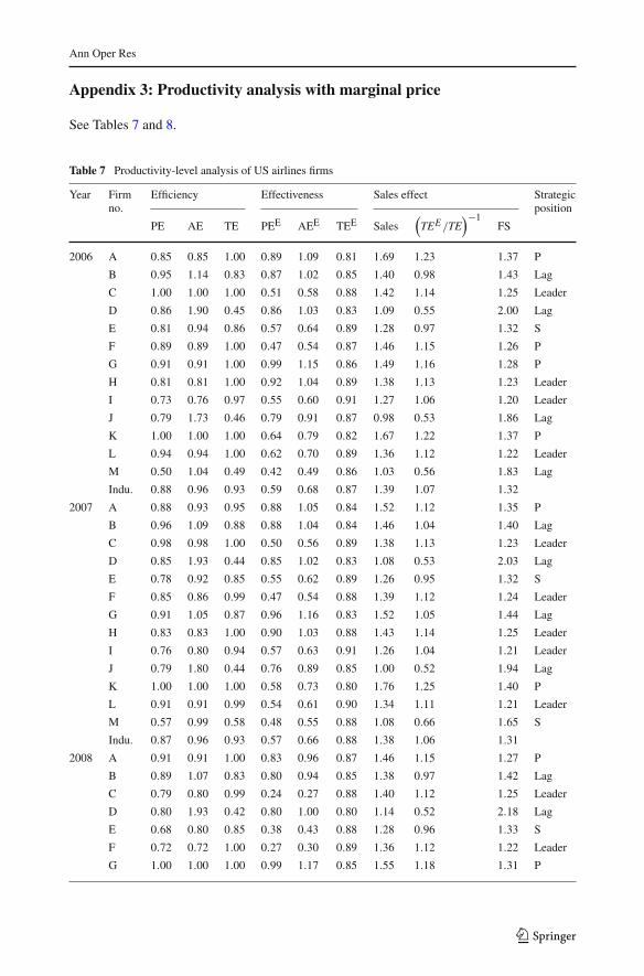
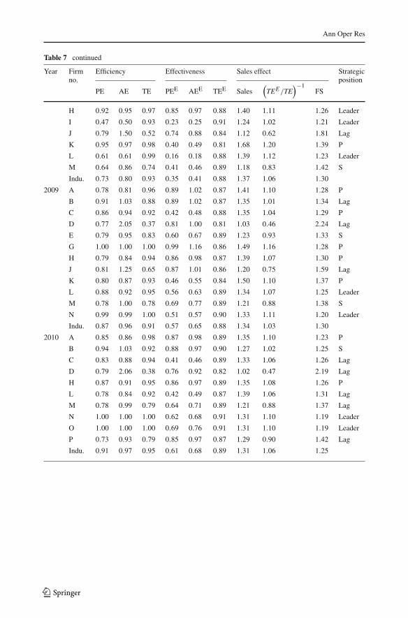
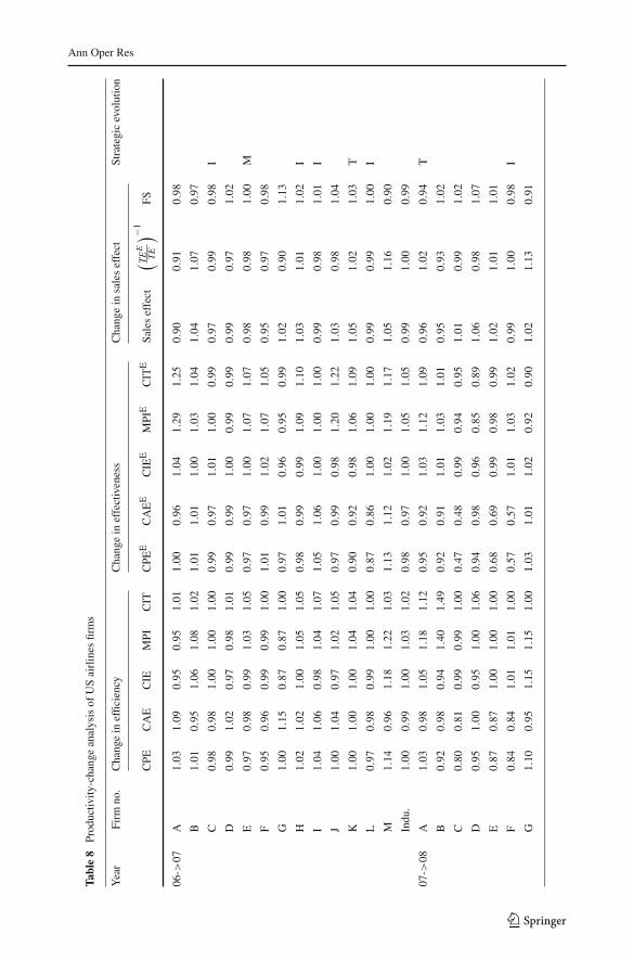
Appendix 3: Productivity analysis with marginal price
See Tables 7 and 8.
Table 7 Productivity-level analysis of US airlines firms
Year Firmno.
Efficiency Effectiveness Sales effect Strategicposition
PE AE TE PEE AEE TEE Sales(
TEE/TE)−1
FS
2006 A 0.85 0.85 1.00 0.89 1.09 0.81 1.69 1.23 1.37 P
B 0.95 1.14 0.83 0.87 1.02 0.85 1.40 0.98 1.43 Lag
C 1.00 1.00 1.00 0.51 0.58 0.88 1.42 1.14 1.25 Leader
D 0.86 1.90 0.45 0.86 1.03 0.83 1.09 0.55 2.00 Lag
E 0.81 0.94 0.86 0.57 0.64 0.89 1.28 0.97 1.32 S
F 0.89 0.89 1.00 0.47 0.54 0.87 1.46 1.15 1.26 P
G 0.91 0.91 1.00 0.99 1.15 0.86 1.49 1.16 1.28 P
H 0.81 0.81 1.00 0.92 1.04 0.89 1.38 1.13 1.23 Leader
I 0.73 0.76 0.97 0.55 0.60 0.91 1.27 1.06 1.20 Leader
J 0.79 1.73 0.46 0.79 0.91 0.87 0.98 0.53 1.86 Lag
K 1.00 1.00 1.00 0.64 0.79 0.82 1.67 1.22 1.37 P
L 0.94 0.94 1.00 0.62 0.70 0.89 1.36 1.12 1.22 Leader
M 0.50 1.04 0.49 0.42 0.49 0.86 1.03 0.56 1.83 Lag
Indu. 0.88 0.96 0.93 0.59 0.68 0.87 1.39 1.07 1.32
2007 A 0.88 0.93 0.95 0.88 1.05 0.84 1.52 1.12 1.35 P
B 0.96 1.09 0.88 0.88 1.04 0.84 1.46 1.04 1.40 Lag
C 0.98 0.98 1.00 0.50 0.56 0.89 1.38 1.13 1.23 Leader
D 0.85 1.93 0.44 0.85 1.02 0.83 1.08 0.53 2.03 Lag
E 0.78 0.92 0.85 0.55 0.62 0.89 1.26 0.95 1.32 S
F 0.85 0.86 0.99 0.47 0.54 0.88 1.39 1.12 1.24 Leader
G 0.91 1.05 0.87 0.96 1.16 0.83 1.52 1.05 1.44 Lag
H 0.83 0.83 1.00 0.90 1.03 0.88 1.43 1.14 1.25 Leader
I 0.76 0.80 0.94 0.57 0.63 0.91 1.26 1.04 1.21 Leader
J 0.79 1.80 0.44 0.76 0.89 0.85 1.00 0.52 1.94 Lag
K 1.00 1.00 1.00 0.58 0.73 0.80 1.76 1.25 1.40 P
L 0.91 0.91 0.99 0.54 0.61 0.90 1.34 1.11 1.21 Leader
M 0.57 0.99 0.58 0.48 0.55 0.88 1.08 0.66 1.65 S
Indu. 0.87 0.96 0.93 0.57 0.66 0.88 1.38 1.06 1.31
2008 A 0.91 0.91 1.00 0.83 0.96 0.87 1.46 1.15 1.27 P
B 0.89 1.07 0.83 0.80 0.94 0.85 1.38 0.97 1.42 Lag
C 0.79 0.80 0.99 0.24 0.27 0.88 1.40 1.12 1.25 Leader
D 0.80 1.93 0.42 0.80 1.00 0.80 1.14 0.52 2.18 Lag
E 0.68 0.80 0.85 0.38 0.43 0.88 1.28 0.96 1.33 S
F 0.72 0.72 1.00 0.27 0.30 0.89 1.36 1.12 1.22 Leader
G 1.00 1.00 1.00 0.99 1.17 0.85 1.55 1.18 1.31 P
123
Ann Oper Res
Table 7 continued
Year Firmno.
Efficiency Effectiveness Sales effect Strategicposition
PE AE TE PEE AEE TEE Sales(
TEE/TE)−1
FS
H 0.92 0.95 0.97 0.85 0.97 0.88 1.40 1.11 1.26 Leader
I 0.47 0.50 0.93 0.23 0.25 0.91 1.24 1.02 1.21 Leader
J 0.79 1.50 0.52 0.74 0.88 0.84 1.12 0.62 1.81 Lag
K 0.95 0.97 0.98 0.40 0.49 0.81 1.68 1.20 1.39 P
L 0.61 0.61 0.99 0.16 0.18 0.88 1.39 1.12 1.23 Leader
M 0.64 0.86 0.74 0.41 0.46 0.89 1.18 0.83 1.42 S
Indu. 0.73 0.80 0.93 0.35 0.41 0.88 1.37 1.06 1.30
2009 A 0.78 0.81 0.96 0.89 1.02 0.87 1.41 1.10 1.28 P
B 0.91 1.03 0.88 0.89 1.02 0.87 1.35 1.01 1.34 Lag
C 0.86 0.94 0.92 0.42 0.48 0.88 1.35 1.04 1.29 P
D 0.77 2.05 0.37 0.81 1.00 0.81 1.03 0.46 2.24 Lag
E 0.79 0.95 0.83 0.60 0.67 0.89 1.23 0.93 1.33 S
G 1.00 1.00 1.00 0.99 1.16 0.86 1.49 1.16 1.28 P
H 0.79 0.84 0.94 0.86 0.98 0.87 1.39 1.07 1.30 P
J 0.81 1.25 0.65 0.87 1.01 0.86 1.20 0.75 1.59 Lag
K 0.80 0.87 0.93 0.46 0.55 0.84 1.50 1.10 1.37 P
L 0.88 0.92 0.95 0.56 0.63 0.89 1.34 1.07 1.25 Leader
M 0.78 1.00 0.78 0.69 0.77 0.89 1.21 0.88 1.38 S
N 0.99 0.99 1.00 0.51 0.57 0.90 1.33 1.11 1.20 Leader
Indu. 0.87 0.96 0.91 0.57 0.65 0.88 1.34 1.03 1.30
2010 A 0.85 0.86 0.98 0.87 0.98 0.89 1.35 1.10 1.23 P
B 0.94 1.03 0.92 0.88 0.97 0.90 1.27 1.02 1.25 S
C 0.83 0.88 0.94 0.41 0.46 0.89 1.33 1.06 1.26 Lag
D 0.79 2.06 0.38 0.76 0.92 0.82 1.02 0.47 2.19 Lag
H 0.87 0.91 0.95 0.86 0.97 0.89 1.35 1.08 1.26 P
L 0.78 0.84 0.92 0.42 0.49 0.87 1.39 1.06 1.31 Lag
M 0.78 0.99 0.79 0.64 0.71 0.89 1.21 0.88 1.37 Lag
N 1.00 1.00 1.00 0.62 0.68 0.91 1.31 1.10 1.19 Leader
O 1.00 1.00 1.00 0.69 0.76 0.91 1.31 1.10 1.19 Leader
P 0.73 0.93 0.79 0.85 0.97 0.87 1.29 0.90 1.42 Lag
Indu. 0.91 0.97 0.95 0.61 0.68 0.89 1.31 1.06 1.25
123
Ann Oper Res
Table8
Productiv
ity-changeanalysisof
USairlines
firms
Year
Firm
no.
Changein
efficiency
Changein
effectiveness
Changein
saleseffect
Strategicevolution
CPE
CAE
CIE
MPI
CIT
CPE
ECAEE
CIE
EMPI
ECIT
ESaleseffect
(TEE
TE
)−1
FS
06->
07A
1.03
1.09
0.95
0.95
1.01
1.00
0.96
1.04
1.29
1.25
0.90
0.91
0.98
B1.01
0.95
1.06
1.08
1.02
1.01
1.01
1.00
1.03
1.04
1.04
1.07
0.97
C0.98
0.98
1.00
1.00
1.00
0.99
0.97
1.01
1.00
0.99
0.97
0.99
0.98
I
D0.99
1.02
0.97
0.98
1.01
0.99
0.99
1.00
0.99
0.99
0.99
0.97
1.02
E0.97
0.98
0.99
1.03
1.05
0.97
0.97
1.00
1.07
1.07
0.98
0.98
1.00
M
F0.95
0.96
0.99
0.99
1.00
1.01
0.99
1.02
1.07
1.05
0.95
0.97
0.98
G1.00
1.15
0.87
0.87
1.00
0.97
1.01
0.96
0.95
0.99
1.02
0.90
1.13
H1.02
1.02
1.00
1.05
1.05
0 .98
0.99
0.99
1.09
1.10
1.03
1.01
1.02
I
I1.04
1.06
0.98
1.04
1.07
1.05
1.06
1.00
1.00
1.00
0.99
0.98
1.01
I
J1.00
1.04
0.97
1.02
1.05
0.97
0.99
0.98
1.20
1.22
1.03
0.98
1.04
K1.00
1.00
1.00
1.04
1.04
0.90
0.92
0.98
1.06
1.09
1.05
1.02
1.03
T
L0.97
0.98
0.99
1.00
1.00
0.87
0.86
1.00
1.00
1.00
0.99
0.99
1.00
I
M1.14
0.96
1.18
1.22
1.03
1.13
1.12
1.02
1.19
1.17
1.05
1.16
0.90
Indu
.1.00
0.99
1.00
1.03
1.02
0.98
0.97
1.00
1.05
1.05
0.99
1.00
0.99
07->
08A
1.03
0.98
1.05
1.18
1.12
0.95
0.92
1.03
1.12
1.09
0.96
1.02
0.94
T
B0.92
0.98
0.94
1.40
1.49
0.92
0.91
1.01
1.03
1.01
0.95
0.93
1.02
C0.80
0.81
0.99
0.99
1.00
0.47
0.48
0.99
0.94
0.95
1.01
0.99
1.02
D0.95
1.00
0.95
1.00
1.06
0.94
0.98
0.96
0.85
0.89
1.06
0.98
1.07
E0.87
0.87
1.00
1.00
1.00
0.68
0.69
0 .99
0.98
0.99
1.02
1.01
1.01
F0.84
0.84
1.01
1.01
1.00
0.57
0.57
1.01
1.03
1.02
0.99
1.00
0.98
I
G1.10
0.95
1.15
1.15
1.00
1.03
1.01
1.02
0.92
0.90
1.02
1.13
0.91
123
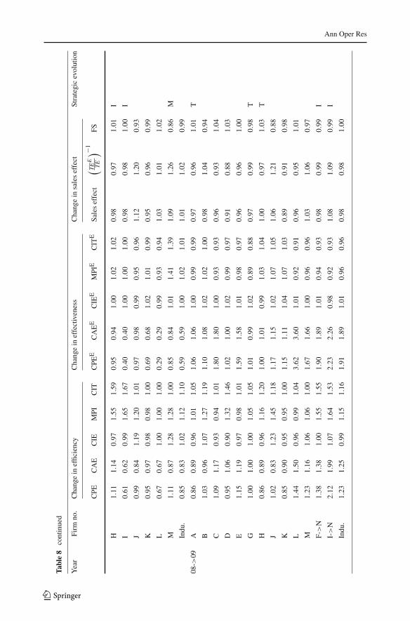
Ann Oper Res
Table8
continued
Year
Firm
no.
Changein
efficiency
Changein
effectiveness
Changein
saleseffect
Strategicevolution
CPE
CAE
CIE
MPI
CIT
CPE
ECAEE
CIE
EMPI
ECIT
ESaleseffect
(TEE
TE
)−1
FS
H1.11
1.14
0.97
1.55
1.59
0.95
0.94
1.00
1.02
1.02
0.98
0.97
1.01
I
I0.61
0.62
0.99
1.65
1.67
0.40
0.40
1.00
1.00
1.00
0.98
0.98
1.00
I
J0.99
0.84
1.19
1.20
1.01
0.97
0.98
0.99
0.95
0.96
1.12
1.20
0.93
K0.95
0.97
0.98
0.98
1.00
0.69
0.68
1.02
1.01
0.99
0.95
0.96
0.99
L0.67
0.67
1.00
1.00
1.00
0.29
0.29
0.99
0.93
0.94
1.03
1.01
1.02
M1.11
0.87
1.28
1.28
1.00
0.85
0.84
1.01
1.41
1.39
1.09
1.26
0.86
M
Indu
.0.85
0.83
1.02
1.12
1.10
0.59
0.59
1.00
1.02
1.01
1.01
1.02
0.99
08->
09A
0.86
0.89
0.96
1.01
1.05
1 .06
1.06
1.00
0.99
0.99
0.97
0.96
1.01
T
B1.03
0.96
1.07
1.27
1.19
1.10
1.08
1.02
1.02
1.00
0.98
1.04
0.94
C1.09
1.17
0.93
0.94
1.01
1.80
1.80
1.00
0.93
0.93
0.96
0.93
1.04
D0.95
1.06
0.90
1.32
1.46
1.02
1.00
1.02
0.99
0.97
0.91
0.88
1.03
E1.15
1.19
0.97
0.98
1.01
1.59
1.58
1.01
0.98
0.97
0.96
0.96
1.00
G1.00
1.00
1.00
1.05
1.05
1.01
0.99
1.02
0.89
0.88
0.97
0.99
0.98
T
H0.86
0.89
0.96
1.16
1.20
1.00
1.01
0.99
1.03
1.04
1.00
0.97
1.03
T
J1.02
0.83
1.23
1.45
1.18
1.17
1.15
1.02
1.07
1.05
1.06
1.21
0.88
K0.85
0.90
0.95
0.95
1.00
1.15
1.11
1.04
1.07
1.03
0.89
0.91
0.98
L1.44
1.50
0.96
0.99
1.04
3.62
3.60
1.01
0.92
0.91
0.96
0.95
1.01
M1.23
1.16
1.06
1.06
1.00
1.67
1.66
1.00
0.96
0.96
1.03
1.06
0.97
F->N
1.38
1.38
1.00
1.55
1.55
1.90
1.89
1 .01
0.94
0.93
0.98
0.99
0.99
I
I->N
2.12
1.99
1.07
1.64
1.53
2.23
2.26
0.98
0.92
0.93
1.08
1.09
0.99
I
Indu
.1.23
1.25
0.99
1.15
1.16
1.91
1.89
1.01
0.96
0.96
0.98
0.98
1.00
123
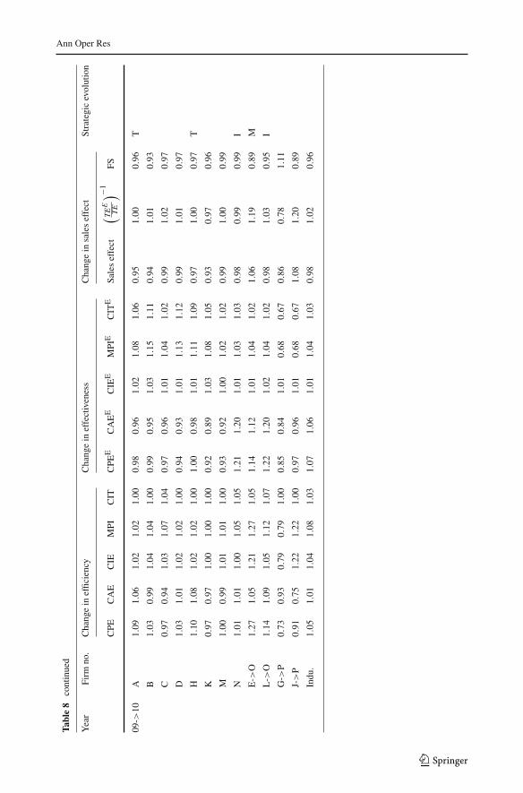
Ann Oper Res
Table8
continued
Year
Firm
no.
Changein
efficiency
Changein
effectiveness
Changein
saleseffect
Strategicevolution
CPE
CAE
CIE
MPI
CIT
CPE
ECAEE
CIE
EMPI
ECIT
ESaleseffect
(TEE
TE
)−1
FS
09->
10A
1.09
1.06
1.02
1.02
1.00
0.98
0.96
1.02
1.08
1.06
0.95
1.00
0.96
T
B1.03
0.99
1.04
1.04
1.00
0.99
0.95
1.03
1.15
1.11
0.94
1.01
0.93
C0.97
0.94
1.03
1.07
1.04
0.97
0.96
1.01
1.04
1.02
0.99
1.02
0.97
D1.03
1.01
1.02
1.02
1.00
0.94
0.93
1.01
1.13
1.12
0.99
1.01
0.97
H1.10
1.08
1.02
1.02
1.00
1.00
0.98
1.01
1.11
1.09
0.97
1.00
0.97
T
K0.97
0.97
1.00
1.00
1.00
0.92
0.89
1.03
1.08
1.05
0.93
0.97
0.96
M1.00
0.99
1.01
1.01
1.00
0.93
0.92
1.00
1.02
1.02
0.99
1.00
0.99
N1.01
1.01
1.00
1.05
1.05
1 .21
1.20
1.01
1.03
1.03
0.98
0.99
0.99
I
E->
O1.27
1.05
1.21
1.27
1.05
1.14
1.12
1.01
1.04
1.02
1.06
1.19
0.89
M
L->
O1.14
1.09
1.05
1.12
1.07
1.22
1.20
1.02
1.04
1.02
0.98
1.03
0.95
I
G->
P0.73
0.93
0.79
0.79
1.00
0.85
0.84
1.01
0.68
0.67
0.86
0.78
1 .11
J->P
0.91
0.75
1.22
1.22
1.00
0.97
0.96
1.01
0.68
0.67
1.08
1.20
0.89
Indu
.1.05
1.01
1.04
1.08
1.03
1.07
1.06
1.01
1.04
1.03
0.98
1.02
0.96
123
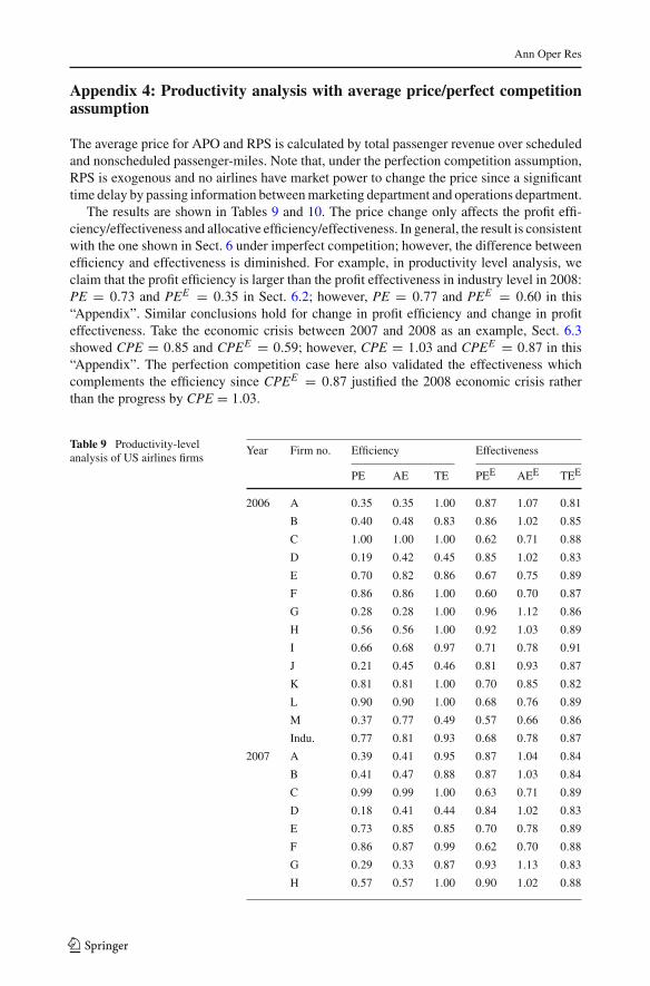
Ann Oper Res
Appendix 4: Productivity analysis with average price/perfect competitionassumption
The average price for APO and RPS is calculated by total passenger revenue over scheduledand nonscheduled passenger-miles. Note that, under the perfection competition assumption,RPS is exogenous and no airlines have market power to change the price since a significanttime delay by passing information betweenmarketing department and operations department.
The results are shown in Tables 9 and 10. The price change only affects the profit effi-ciency/effectiveness and allocative efficiency/effectiveness. In general, the result is consistentwith the one shown in Sect. 6 under imperfect competition; however, the difference betweenefficiency and effectiveness is diminished. For example, in productivity level analysis, weclaim that the profit efficiency is larger than the profit effectiveness in industry level in 2008:PE = 0.73 and PEE = 0.35 in Sect. 6.2; however, PE = 0.77 and PEE = 0.60 in this“Appendix”. Similar conclusions hold for change in profit efficiency and change in profiteffectiveness. Take the economic crisis between 2007 and 2008 as an example, Sect. 6.3showed CPE = 0.85 and CPEE = 0.59; however, CPE = 1.03 and CPEE = 0.87 in this“Appendix”. The perfection competition case here also validated the effectiveness whichcomplements the efficiency since CPEE = 0.87 justified the 2008 economic crisis ratherthan the progress by CPE = 1.03.
Table 9 Productivity-levelanalysis of US airlines firms
Year Firm no. Efficiency Effectiveness
PE AE TE PEE AEE TEE
2006 A 0.35 0.35 1.00 0.87 1.07 0.81
B 0.40 0.48 0.83 0.86 1.02 0.85
C 1.00 1.00 1.00 0.62 0.71 0.88
D 0.19 0.42 0.45 0.85 1.02 0.83
E 0.70 0.82 0.86 0.67 0.75 0.89
F 0.86 0.86 1.00 0.60 0.70 0.87
G 0.28 0.28 1.00 0.96 1.12 0.86
H 0.56 0.56 1.00 0.92 1.03 0.89
I 0.66 0.68 0.97 0.71 0.78 0.91
J 0.21 0.45 0.46 0.81 0.93 0.87
K 0.81 0.81 1.00 0.70 0.85 0.82
L 0.90 0.90 1.00 0.68 0.76 0.89
M 0.37 0.77 0.49 0.57 0.66 0.86
Indu. 0.77 0.81 0.93 0.68 0.78 0.87
2007 A 0.39 0.41 0.95 0.87 1.04 0.84
B 0.41 0.47 0.88 0.87 1.03 0.84
C 0.99 0.99 1.00 0.63 0.71 0.89
D 0.18 0.41 0.44 0.84 1.02 0.83
E 0.73 0.85 0.85 0.70 0.78 0.89
F 0.86 0.87 0.99 0.62 0.70 0.88
G 0.29 0.33 0.87 0.93 1.13 0.83
H 0.57 0.57 1.00 0.90 1.02 0.88
123
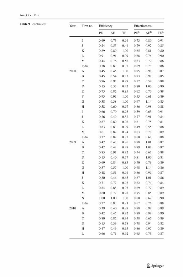
Ann Oper Res
Table 9 continued Year Firm no. Efficiency Effectiveness
PE AE TE PEE AEE TEE
I 0.69 0.73 0.94 0.73 0.80 0.91
J 0.24 0.55 0.44 0.79 0.92 0.85
K 0.89 0.89 1.00 0.65 0.81 0.80
L 0.91 0.91 0.99 0.68 0.76 0.90
M 0.44 0.76 0.58 0.63 0.72 0.88
Indu. 0.78 0.83 0.93 0.69 0.79 0.88
2008 A 0.45 0.45 1.00 0.85 0.98 0.87
B 0.45 0.54 0.83 0.83 0.97 0.85
C 0.96 0.97 0.99 0.52 0.59 0.88
D 0.15 0.37 0.42 0.80 1.00 0.80
E 0.73 0.85 0.85 0.62 0.70 0.88
F 0.93 0.93 1.00 0.55 0.61 0.89
G 0.38 0.38 1.00 0.97 1.14 0.85
H 0.58 0.60 0.97 0.86 0.98 0.88
I 0.66 0.70 0.93 0.59 0.65 0.91
J 0.26 0.49 0.52 0.77 0.91 0.84
K 0.87 0.89 0.98 0.61 0.75 0.81
L 0.83 0.83 0.99 0.49 0.55 0.88
M 0.61 0.82 0.74 0.63 0.70 0.89
Indu. 0.77 0.82 0.93 0.60 0.68 0.88
2009 A 0.42 0.43 0.96 0.88 1.01 0.87
B 0.42 0.48 0.88 0.89 1.02 0.87
C 0.83 0.91 0.92 0.54 0.62 0.88
D 0.15 0.40 0.37 0.81 1.00 0.81
E 0.69 0.84 0.83 0.70 0.79 0.89
G 0.57 0.57 1.00 0.98 1.14 0.86
H 0.48 0.51 0.94 0.86 0.99 0.87
J 0.30 0.46 0.65 0.87 1.01 0.86
K 0.71 0.77 0.93 0.62 0.74 0.84
L 0.84 0.88 0.95 0.69 0.77 0.89
M 0.60 0.77 0.78 0.75 0.85 0.89
N 1.00 1.00 1.00 0.60 0.67 0.90
Indu. 0.77 0.83 0.91 0.67 0.76 0.88
2010 A 0.39 0.40 0.98 0.88 0.98 0.89
B 0.42 0.45 0.92 0.89 0.98 0.90
C 0.80 0.85 0.94 0.58 0.65 0.89
D 0.15 0.39 0.38 0.78 0.94 0.82
H 0.47 0.49 0.95 0.86 0.97 0.89
L 0.66 0.71 0.92 0.65 0.75 0.87
123
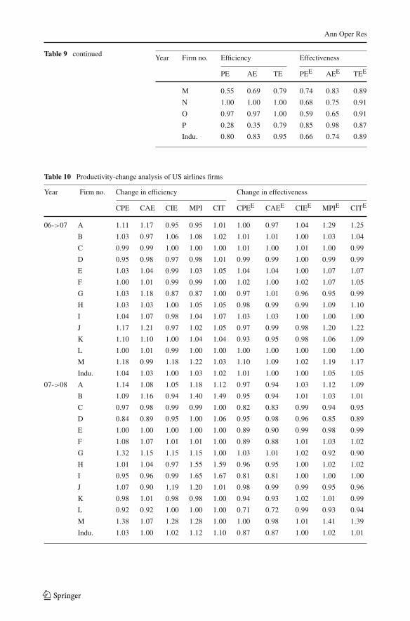
Ann Oper Res
Table 9 continued Year Firm no. Efficiency Effectiveness
PE AE TE PEE AEE TEE
M 0.55 0.69 0.79 0.74 0.83 0.89
N 1.00 1.00 1.00 0.68 0.75 0.91
O 0.97 0.97 1.00 0.59 0.65 0.91
P 0.28 0.35 0.79 0.85 0.98 0.87
Indu. 0.80 0.83 0.95 0.66 0.74 0.89
Table 10 Productivity-change analysis of US airlines firms
Year Firm no. Change in efficiency Change in effectiveness
CPE CAE CIE MPI CIT CPEE CAEE CIEE MPIE CITE
06->07 A 1.11 1.17 0.95 0.95 1.01 1.00 0.97 1.04 1.29 1.25
B 1.03 0.97 1.06 1.08 1.02 1.01 1.01 1.00 1.03 1.04
C 0.99 0.99 1.00 1.00 1.00 1.01 1.00 1.01 1.00 0.99
D 0.95 0.98 0.97 0.98 1.01 0.99 0.99 1.00 0.99 0.99
E 1.03 1.04 0.99 1.03 1.05 1.04 1.04 1.00 1.07 1.07
F 1.00 1.01 0.99 0.99 1.00 1.02 1.00 1.02 1.07 1.05
G 1.03 1.18 0.87 0.87 1.00 0.97 1.01 0.96 0.95 0.99
H 1.03 1.03 1.00 1.05 1.05 0.98 0.99 0.99 1.09 1.10
I 1.04 1.07 0.98 1.04 1.07 1.03 1.03 1.00 1.00 1.00
J 1.17 1.21 0.97 1.02 1.05 0.97 0.99 0.98 1.20 1.22
K 1.10 1.10 1.00 1.04 1.04 0.93 0.95 0.98 1.06 1.09
L 1.00 1.01 0.99 1.00 1.00 1.00 1.00 1.00 1.00 1.00
M 1.18 0.99 1.18 1.22 1.03 1.10 1.09 1.02 1.19 1.17
Indu. 1.04 1.03 1.00 1.03 1.02 1.01 1.00 1.00 1.05 1.05
07->08 A 1.14 1.08 1.05 1.18 1.12 0.97 0.94 1.03 1.12 1.09
B 1.09 1.16 0.94 1.40 1.49 0.95 0.94 1.01 1.03 1.01
C 0.97 0.98 0.99 0.99 1.00 0.82 0.83 0.99 0.94 0.95
D 0.84 0.89 0.95 1.00 1.06 0.95 0.98 0.96 0.85 0.89
E 1.00 1.00 1.00 1.00 1.00 0.89 0.90 0.99 0.98 0.99
F 1.08 1.07 1.01 1.01 1.00 0.89 0.88 1.01 1.03 1.02
G 1.32 1.15 1.15 1.15 1.00 1.03 1.01 1.02 0.92 0.90
H 1.01 1.04 0.97 1.55 1.59 0.96 0.95 1.00 1.02 1.02
I 0.95 0.96 0.99 1.65 1.67 0.81 0.81 1.00 1.00 1.00
J 1.07 0.90 1.19 1.20 1.01 0.98 0.99 0.99 0.95 0.96
K 0.98 1.01 0.98 0.98 1.00 0.94 0.93 1.02 1.01 0.99
L 0.92 0.92 1.00 1.00 1.00 0.71 0.72 0.99 0.93 0.94
M 1.38 1.07 1.28 1.28 1.00 1.00 0.98 1.01 1.41 1.39
Indu. 1.03 1.00 1.02 1.12 1.10 0.87 0.87 1.00 1.02 1.01
123
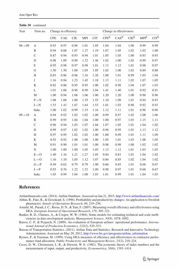
Ann Oper Res
Table 10 continued
Year Firm no. Change in efficiency Change in effectiveness
CPE CAE CIE MPI CIT CPEE CAEE CIEE MPIE CITE
08->09 A 0.93 0.97 0.96 1.01 1.05 1.04 1.04 1.00 0.99 0.99
B 0.94 0.88 1.07 1.27 1.19 1.07 1.05 1.02 1.02 1.00
C 0.87 0.94 0.93 0.94 1.01 1.05 1.05 1.00 0.93 0.93
D 0.98 1.09 0.90 1.32 1.46 1.02 1.00 1.02 0.99 0.97
E 0.95 0.98 0.97 0.98 1.01 1.13 1.12 1.01 0.98 0.97
G 1.50 1.50 1.00 1.05 1.05 1.02 1.00 1.02 0.89 0.88
H 0.83 0.86 0.96 1.16 1.20 1.00 1.01 0.99 1.03 1.04
J 1.16 0.94 1.23 1.45 1.18 1.13 1.11 1.02 1.07 1.05
K 0.82 0.86 0.95 0.95 1.00 1.02 0.98 1.04 1.07 1.03
L 1.01 1.06 0.96 0.99 1.04 1.41 1.40 1.01 0.92 0.91
M 1.00 0.94 1.06 1.06 1.00 1.20 1.20 1.00 0.96 0.96
F->N 1.08 1.08 1.00 1.55 1.55 1.10 1.09 1.01 0.94 0.93
I->N 1.53 1.43 1.07 1.64 1.53 1.01 1.03 0.98 0.92 0.93
Indu. 1.00 1.02 0.99 1.15 1.16 1.12 1.11 1.01 0.96 0.96
09->10 A 0.94 0.92 1.02 1.02 1.00 0.99 0.97 1.02 1.08 1.06
B 0.99 0.95 1.04 1.04 1.00 1.00 0.97 1.03 1.15 1.11
C 0.96 0.94 1.03 1.07 1.04 1.07 1.05 1.01 1.04 1.02
D 0.99 0.97 1.02 1.02 1.00 0.96 0.95 1.01 1.13 1.12
H 0.97 0.95 1.02 1.02 1.00 1.00 0.99 1.01 1.11 1.09
K 0.92 0.92 1.00 1.00 1.00 1.05 1.01 1.03 1.08 1.05
M 0.91 0.90 1.01 1.01 1.00 0.98 0.98 1.00 1.02 1.02
N 1.00 1.00 1.00 1.05 1.05 1.13 1.12 1.01 1.03 1.03
E->O 1.40 1.16 1.21 1.27 1.05 0.84 0.83 1.01 1.04 1.02
L->O 1.16 1.10 1.05 1.12 1.07 0.86 0.85 1.02 1.04 1.02
G->P 0.49 0.62 0.79 0.79 1.00 0.86 0.85 1.01 0.68 0.67
J->P 0.93 0.76 1.22 1.22 1.00 0.98 0.97 1.01 0.68 0.67
Indu. 1.03 0.99 1.04 1.08 1.03 1.01 0.99 1.01 1.04 1.03
References
Airlinefinancials.com. (2014). Airline Database. Assessed on Jan 21, 2015, http://www.airlinefinancials.com/Althin, R., Färe, R., & Grosskopf, S. (1996). Profitability and productivity changes: An application to Swedish
pharmacies. Annals of Operations Research, 66, 219–230.Asmild, M., Paradi, J. C., Reese, D. N., & Tam, F. (2007). Measuring overall efficiency and effectiveness using
DEA. European Journal of Operational Research, 178, 305–321.Banker, R. D., Charnes, A., & Cooper, W. W. (1984). Some models for estimating technical and scale ineffi-
ciencies in data envelopment analysis. Management Science, 30(9), 1078–1092.Barros, C. P., & Peypoch, N. (2009). An evaluation of European airlines’ operational performance. Interna-
tional Journal of Production Economics, 122(2), 525–533.Bureau of Transportation Statistics. (2011). Airline Data and Statistics, Research and Innovative Technology
Administration. Assessed on May 29, 2012, http://www.bts.gov/programs/airline_informationByrnes, P., & Freeman, M. (1999). Using DEA measures of efficiency and effectiveness in contractor perfor-
mance fund allocation. Public Productivity and Management Review, 23(2), 210–224.Caves, D. W., Christensen, L. R., & Diewert, W. E. (1982). The economic theory of index numbers and the
measurement of input, output, and productivity. Econometrica, 50(6), 1393–1414.
123
Ann Oper Res
Charnes, A., Cooper,W.W.,&Rhodes, E. (1978).Measuring the efficiency of decisionmaking units.EuropeanJournal of Operational Research, 2(6), 429–444.
Chen, W.-C., &McGinnis, L. F. (2007). Reconciling ratio analysis and DEA as performance assessment tools.European Journal of Operational Research, 178(1), 277–291.
Coelli, T. J., Rao, D. S. P., O’Donnell, C. J., & Battese, G. E. (2005). An introduction to efficiency andproductivity analysis (2nd ed.). New York: Springer.
Diewert, W. E. (1980). Capital and the theory of productivity measurement. The American Economic Review,70(2), 260–267.
Diewert, W. E. (1992). The measurement of productivity. Bulletin of Economic Research, 44(3), 163–198.Färe, R., Grosskopf, S., Lindgren, B., & Roos, P. (1992). Productivity changes in Swedish pharmacies 1980–
1989: A non-parametric Malmquist approach. Journal of Productivity Analysis, 3(1–2), 85–101.Färe, R., Grosskopf, S., Norris, M., & Zhang, Z. (1994). Productivity growth technical progress, and efficiency
change in industrialized countries. American Economic Review, 84(1), 66–83.Farrell, M. J. (1957). The measurement of productive efficiency. Journal of the Royal Statistical Society Series
A, 120(3), 253–290.Fielding, G. J., Babitsky, T. T., &Brenner,M. E. (1985). Performance evaluation for bus transit. Transportation
Research Part A, 19(1), 73–82.Golany, B. (1988). An interactiveMOLP procedure for the extension of DEA to effectiveness analysis. Journal
of the Operational Research Society, 39(8), 725–734.Golany,B., Phillips, F.Y.,&Rousseau, J. J. (1993).Models for improved effectiveness based onDEAefficiency
results. IIE Transactions, 25(6), 2–10.Golany, B., & Tamir, E. (1995). Evaluating efficiency-effectiveness-equality trade-offs: a data envelopment
analysis approach.Management Science, 41(7), 1172–1184.Graf, M., & Kimms, A. (2013). Transfer price optimization for option-based airline alliance revenue manage-
ment. International Journal of Production Economics, 145, 281–293.Grifell-Tatjé, E., & Lovell, C. A. K. (1997). A DEA-based analysis of productivity change and intertemporal
managerial performance. Annals of Operations Research, 73, 177–189.Hildreth, C. (1954). Point estimates of ordinates of concave functions. Journal of the American Statistical
Association, 49(267), 598–619.IATA. (2010). 2009: Worst demand decline in history—encouraging year-end improvements. Assessed on
May 29, 2012, http://www.iata.org/pressroom/pr/Pages/2010-01-27-01.aspxKuosmanen, T. (2008). Representation theorem for convex nonparametric least squares.Econometrics Journal,
11(2), 308–325.Kuosmanen, T. (2012). Stochastic semi-nonparametric frontier estimation of electricity distribution networks:
Application of the StoNED method in the Finnish regulatory model. Energy Economics, 34(6), 2189–2199.
Kuosmanen, T., & Johnson, A. L. (2010). Data envelopment analysis as nonparametric least squares regression.Operations Research, 58(1), 149–160.
Lee, C.-Y., & Johnson, A. L. (2011). A decomposition of productivity change in the semiconductor manufac-turing industry. International Journal of Production Research, 49(16), 4761–4785.
Lee, C.-Y., & Johnson, A. L. (2012). Two-dimensional efficiency decomposition to measure the demand effectin productivity analysis. European Journal of Operational Research, 216(3), 584–593.
Lee, C.-Y., & Johnson, A. L. (2014). Proactive data envelopment analysis: Effective production and capacityexpansion in stochastic environments. European Journal of Operational Research, 232(3), 537–548.
Lee, C.-Y., & Johnson, A. L. (2015). Measuring efficiency in imperfectly competitive markets: An exampleof rational inefficiency. Journal of Optimization Theory and Applications, 164(2), 702–722.
Lovell, C. A. K., & Rouse, A. P. B. (2003). Equivalent standard DEA models to provide super-efficiencyscores. Journal of the Operational Research Society, 54, 101–108.
Nerlove, M. (1965). Estimation and identification of Cobb–Douglas production functions. Chicago: Rand-McNally.
Ouellette, P., & Vierstraete, V. (2010). Malmquist indexes with quasi-fixed inputs: An application to schooldistricts in Québec. Annals of Operations Research, 173(1), 57–76.
Semenick Alam, I., & Sickles, R. (2000). Time series analysis of deregulatory dynamics and technical effi-ciency: The case of the US airline industry. International Economic Review, 41(1), 203–218.
Talluri, S., Narasimhan, R., & Nair, A. (2006). Vendor performance with supply risk: A chance-constrainedDEA approach. International Journal of Production Economics, 100(2), 212–222.
Vaz, C. B., Camanho, A. S., & Guimarães, R. C. (2010). The assessment of retailing efficiency using networkdata envelopment analysis. Annals of Operations Research, 173(1), 5–24.
Yu, M.-M., & Lin, E. T. J. (2008). Efficiency and effectiveness in railway performance using a multiactivitynetwork DEA model. Omega, 36(6), 1005–1017.
123