effectoffree-stream turbulenceonboundarylayer...

rsta.royalsocietypublishing.org

ReviewCite this article: Goldstein ME. 2014 Effect offree-stream turbulence on boundary layertransition. Phil. Trans. R. Soc. A 372: 20130354.http://dx.doi.org/10.1098/rsta.2013.0354

One contribution of 15 to a Theme Issue‘Stability, separation and close bodyinteractions’.

Subject Areas:fluid mechanics

Keywords:boundary layer transition, free-streamturbulence, boundary layer streaks

Author for correspondence:M. E. Goldsteine-mail: [email protected]

Effect of free-streamturbulence on boundary layertransitionM. E. Goldstein

NASA Glenn Research Center, 2100 Brookpark Road, Cleveland,44135 OH, USA

This paper is concerned with the transition toturbulence in flat plate boundary layers due tomoderately high levels of free-stream turbulence.The turbulence is assumed to be generated by an(idealized) grid and matched asymptotic expansionsare used to analyse the resulting flow over a finitethickness flat plate located in the downstream region.The characteristic Reynolds number RΛ based on themesh size Λ and free-stream velocity is assumed tobe large, and the turbulence intensity ε is assumed tobe small. The asymptotic flow structure is discussedfor the generic case where the turbulence Reynoldsnumber εRΛ and the plate thickness and are held fixed(at O(1) and O(Λ), respectively) in the limit as RΛ → ∞and ε→ 0. But various limiting cases are considered inorder to explain the relevant transition mechanisms.It is argued that there are two types of streak-likestructures that can play a role in the transition process:(i) those that appear in the downstream region and aregenerated by streamwise vorticity in upstream flowand (ii) those that are concentrated near the leadingedge and are generated by plate normal vorticity inupstream flow. The former are relatively unaffected byleading edge geometry and are usually referred to asKlebanoff modes while the latter are strongly affectedby leading edge geometry and are more streamwisevortex-like in appearance.

1. IntroductionThis paper is concerned with the transition to turbulencein flat plate boundary layers due to moderately highlevels of grid-generated turbulence—a subject that beganwith the work of Dryden [1] and Taylor [2], who showedthat the unsteady boundary layer flow was dominatedby chaotic low-frequency streaks. But these studies werelargely ignored by subsequent researchers who focused

2014 The Author(s) Published by the Royal Society. All rights reserved.

on July 3, 2018http://rsta.royalsocietypublishing.org/Downloaded from

http://crossmark.crossref.org/dialog/?doi=10.1098/rsta.2013.0354&domain=pdf&date_stamp=2014-06-16

mailto:[email protected]

http://rsta.royalsocietypublishing.org/

2

rsta.royalsocietypublishing.orgPhil.Trans.R.Soc.A372:20130354

.........................................................

y*

z*

U•

w• = e U• cos (2 p z*/L)

x*

d

L

Figure 1. Configuration for Crow’s analysis.

on the much more regular and (at the time) seemingly more interesting Tollmien–Schlichtingwaves that occur at very low free-stream turbulence levels (say less than 1% or so) until theseearlier ideas were resurrected about two decades later by Klebanoff [3]. However, the researchreally took off in the late 1980s and 1990s. Klebanoff found that the measured hot wire signalthat passed through a low-pass filter at 12 Hz was almost identical in magnitude to the signalmeasured over all frequencies, indicating that most of the energy was in frequencies below12 Hz—a result that has now been reproduced many times. Kendall [4] later showed that thespanwise dimension of these low-frequency structures, which he referred to as Klebanoff modes,was of the order of the boundary layer thickness. Based on an earlier proposal that Bradshaw [5]introduced to explain some low free-stream turbulence observations, Klebanoff [3] suggested thatthese ‘modes’ (which, as has been pointed out many times, are not actually eigenmodes) could beinterpreted as a local thickening and thinning of the Blasius boundary layer. Bradshaw [5] pointedout that perturbing the boundary layer thickness, say δ, in the Blasius solution, u = F′

B(η) (wherethe prime denotes differentiation with respect to η= y/δ and FB is the Blasius function) by a smallamount, say δ(1), and expanding in a Taylor series gives

u = F′B

(y

δ + δ(1)

)= F′

B(η) − δ(1)

δηF′′

B(η) + · · · , (1.1)

which means that the difference between the actual streamwise velocity u and the Blasiussolution should be proportional to ηF′′

B—a result that is almost invariably found to be in excellentagreement with experimental observations.

A few months after Bradshaw came up with this proposal Crow [6], who had been visitingthe National Physical Laboratory, Teddington, UK, at the time, put this result on a more rigorousfoundation by analysing the flow over an infinitely thin flat plate produced by a small-amplitudespanwise-periodic velocity perturbation

w∞ = ε cos(

2πz∗

Λ

), (1.2)

imposed on a uniform upstream flow U∞, where ε is a measure of the disturbance amplitude(figure 1).

His analysis showed that

u = F′B(η) − 1

2

[ε

(x∗

Λ

)sin

(2πz∗

Λ

)]ηF′′

B(η), (1.3)



3


.........................................................

y*

z*

x*

I IIIV V

III

III

U•

O (L)

Ls/e

(x, y, z) = {x*, y*, z*}/L

eu•(x – t, y, z;t )

L

L

L

V

flat plate

Figure 2. Generic flow configuration.

when δ�Λ, which means that the boundary layer thickness perturbation δ(1) in (1.1) should begiven by δ(1) = [εδ(x∗/Λ) sin(2πz∗/Λ)]/2. While this is a remarkably simple and elegant result, itdoes not agree with the experimentally observed growth rate, which seems to be more like

√x∗

than like x∗.There is obviously a lot more about Klebanoff modes and their subsequent breakdown into

turbulence that still needs to be explained. This paper attempts to give an overview of a verygeneral methodology that has been developed to provide this explanation. Most of the materialhas already appeared in the literature but some new material is included in §§2 (at the end)and 3. An excellent summary of the overall approach can be found in the Introduction of [7],which also provides a penetrating explanation of why the other methodologies proposed in theliterature (optimal growth (see also Introduction of [8]), Orr–Sommerfeld theory, leading edgeeigensolutions, etc.) do not provide viable alternatives to this approach.

2. Overall flow structureThe paper begins by considering the general situation shown in figure 2, but assumes, forsimplicity, that the flow is incompressible [9–11]. The fundamental length-scale Λ is set bythe (idealized) upstream grid, which is presumed to generate weak free-stream turbulencewith characteristic amplitude O(εU∞). It can, therefore, be locally represented by a convecteddisturbance, say εu∞(x − it; t), x = {x, y, z} that satisfies the continuity equation ∇ · u∞ = 0 and canotherwise be specified as an upstream boundary condition [12]. All velocities are assumed to benormalized by the uniform free-stream velocity, U∞, all lengths by Λ, the time, t, by Λ/U∞ and,because of the important role played by the low-frequency disturbances, it seems appropriateto explicitly specify the parametric dependence of u∞ on the slow time variable t ≡ εt/σ , whereσ ε is an additional gauge function. The technologically interesting cases, for which virtuallyall of the experiments were carried out, correspond to large values of the characteristic Reynoldsnumber RΛ ≡ U∞Λ/ν. The generic scaling then corresponds to the double limit as RΛ → ∞, ε→ 0with the turbulence Reynolds number RT ≡ εRΛ and plate thickness held fixed at O(1) and O(Λ),respectively: in which case, the additional gauge function σ = σ (RT) can be set equal to unity andthe flow divides into the five asymptotic regions shown in figure 2.

The flow in region I, which corresponds to the vicinity of the leading edge (i.e. |x| = O(1)),is nearly two dimensional and steady with the three-dimensional and unsteady effects being an



4


.........................................................

O(ε) perturbation of the two-dimensional potential flow, {U0, V0, 0}. The latter is basically inviscidwhen the grid is sufficiently close to the leading edge, which is now assumed to be the case.

The viscous effects are then confined to a relatively thin boundary layer of thickness O(R−1/2Λ ),

which is denoted as region II in the figure and is again nearly two dimensional and steady withthe three-dimensional and unsteady effects coming in as a O(ε) perturbation of that flow. Theflow in region I is governed by linear rapid distortion theory [13–15] about a two-dimensionalpotential mean flow U0 − iV0 = dW/dξ , ξ = x + iy, which is induced by the plate and the O(R−1/2

Λ )displacement effects of the two-dimensional boundary layer flow. The latter can be accounted forby adding−iR−1/2

Λ δ(ξ ), where δ(ξ ) is the analytic continuation into the complex ξ -plane of thescaled boundary layer displacement, to the complex potential W = W0 of the plate itself. Therapid distortion theory solution is easily found by solving a Poisson equation [15].

Asymptotic solutions to the linearized boundary layer problem constructed in [6,11,16] showthat the unsteady flow can be divided into a two-dimensional component that is driven by thestreamwise velocity at the bottom of region I and remains small, i.e. O(ε) for all x, and a three-dimensional component that is driven by the cross flow velocity at the bottom of region I andcontinues to grow with increasing x. Leib et al. [11] constructed a Wentzel–Kramers–Brillouin–Jeffreys solution for this component that is valid in the limit as x → ∞ with t = O(1) and has asingle turning point at the outer edge of the boundary layer [7,11]. Since this solution must breakdown in the vicinity of that point a new asymptotic solution has to be constructed in this region,which is usually referred to as the ‘edge layer’. This result shows that the O(1) frequency velocityperturbations move out into this ‘edge layer’ as x → ∞, while the 1/t = O(ε/σ ) low-frequencyportion of the three-dimensional component of the boundary layer solution continues to growwith increasing x. The smaller transverse wavenumber components exhibit the most rapidgrowth, suggesting that the velocity fluctuations within the boundary layer will be dominatedby the low-frequency small transverse wavenumber components at large downstream distances,where y = O(1) and x = O(σ/ε).

The boundary layer thickness also continues to increase with increasing x and the classicallinearized boundary layer solution (which only applies when the boundary layer thickness ismuch less thanΛ [8]) eventually becomes invalid. A new solution therefore has to be constructedin region III where

x ≡ εxσ

(2.1)

and y are both O(1). The flow is fully nonlinear in this region and the boundary layer thicknessis of the same order as the spanwise wavelength when RT = O(1). It, therefore, scales like {u, p +1/2} = {U, (ε/σ )V, (ε/σ )W, (ε/σ )2P} and is governed by the boundary region equations [17]

∂U∂ t

+ U∂U∂ x

+ V∂U∂y

+ W∂U∂z

= σ

RT

(∂2U∂y2 + ∂2U

∂z2

), (2.2)

∂V∂ t

+ U∂V∂ x

+ V∂V∂y

+ W∂V∂z

= −∂P∂y

+ σ

RT

(∂2V∂y2 + ∂2V

∂z2

)(2.3)

∂W∂ t

+ U∂W∂ x

+ V∂W∂y

+ W∂W∂z

= −∂P∂z

+ σ

RT

(∂2W∂y2 + ∂2W

∂z2

)(2.4)

and∂U∂ x

+ ∂V∂y

+ ∂W∂z

= 0, (2.5)

which are just the Navier–Stokes equations with the streamwise derivatives neglected in theviscous and pressure gradient terms, implying that spanwise ellipticity is important in regionIII. This is the region of primary interest since the spanwise wavelength is of the order of theboundary layer thickness in almost all Klebanoff mode experiments. It is worth noting thatthe spanwise ellipticity (which introduces additional viscous effects) decreases the streamwisegrowth rate of the wall layer streaks below the linear growth rate that occurs in the upstreamboundary layer region II, which explains the discrepancy between the Crow [6] analysis and the



5


.........................................................

experimental observations. It is also worth noting that the definition of the scaled streamwisecoordinate x is somewhat different from the one used in [11], but the two are asymptoticallyequivalent because the scale factors are of the same asymptotic order.

The thin edge layer that causes the high-frequency disturbances to move out of the unsteadyboundary layer region at large downstream distances is expected to continue downstream andform a region V that lies between region III and region IV, where x = O(1) and y ≡ εy = O(1) whenRT = O(1). This layer (which was not included in some of the previous studies) is expected to actas a kind of buffer zone that prevents the high-frequency/small-scale disturbances in region IVfrom penetrating into region III (see [7]). It did not appear in the analyses in [8,18] because theregion IV disturbances were of low frequency or completely steady in those papers, and it wasnot included in [11] because the low-frequency components could be treated independently ofthe high-frequency components in the linearized flow investigated in that paper.

3. Flow in region IVThe flow in this region expands like [8,9,11,18]

u = i + ε

[1σ

u0(x, y, t) + u(x, x; t0)]

+ · · · , (3.1)

where u depends on the slow moving frame variable t0 ≡ t − x only parametrically, the complexconjugate velocity u0 − iv0 of the mean displacement velocity u0 = {u0, v0, 0} is given by [18]

u0 − iv0 = −iδξ (ξ , t), (3.2)

where δ(ξ , t) is the analytic continuation of the displacement thickness

δ ≡ 1T

∫T

0

∫∞

0[1 − U(x, y, z, t)] dy dz (3.3)

into the complex ξ ≡ x + iy plane, and u satisfies the full Navier–Stokes equations

1σ

∂u∂ x

+ u · ∇xu = −∇xp∞ + 1RT

∇2x u (3.4)

and∇x · u = 0, (3.5)

in the slow variable εx (which plays the role of time) and the fast displaced moving coordinatesystem variable

x = {x1, x2, x3} ≡ {x − t + Imδ(ξ , t), y − Reδ(ξ , t), z}, (3.6)

subjected to the upstream boundary condition

u(x, 0; t0) = u∞(x, t0). (3.7)

The operator ∇x is defined in the obvious way by

∇x ≡{∂

∂ x1,∂

∂ x2,∂

∂ x3

}, (3.8)

the modified displacement δ is determined by the first-order partial differential equation

δξ + δ t = δξ , (3.9)

and p∞ denotes the corresponding pressure, but the partial derivatives with respect to x and xi,i = 1, 2, 3 are at constant t0 ≡ t − x, since the slow time variable t0 enters only parametrically. Sothe actual time-dependent velocity at x is given by u(x, x; t − x). And as can be seen by directsubstitution, the displaced streamwise coordinate x1 (which did not enter the correspondingequations in [18] and [8] since the flow was of low frequency or completely steady in thosepapers) had to be introduced in order to balance the advection of streamwise momentum in theNavier–Stokes equation (3.4).



6


.........................................................

As region V is expected to filter out the x − t dependence of the region IV solution, it is likelythat the flow in the viscous wall layer (region III) will be mainly determined by the time-average(low-frequency) component

u(x⊥, x; t0) ≡ lim�→∞

12�

∫�−�

u(x, x; t0) dx1 = limT→∞

12T

∫T

−Tu(x, x; t0) dt, (3.10)

p∞(x⊥, x; t0) ≡ lim�→∞

12�

∫�−�

p∞(x, x; t0) dx1 (3.11)

and x⊥ ≡ {0, x2, x3} (3.12)

of the region IV solution, which satisfies

1σ

∂u∂ x

+ u⊥ · ∇⊥u = −∇⊥p∞ + 1RT

∇2⊥u − ∇⊥ · u′u′ (3.13)

and

∇⊥ · u⊥ = 0, (3.14)

subject to the inhomogeneous upstream boundary condition

u(x⊥, 0; t0) = u∞(x⊥, t0) (3.15)

and is expected to remain relatively inhomogeneous and grid dependent even though the overallturbulence velocity u is expected to be approximately homogeneous. Appropriate transverseboundary conditions can probably be inferred by assuming that u has the same transverseperiodicity as the imposed upstream flow. The remaining quantities in (3.13)–(3.15) are definedby

u′ ≡ u − u, (3.16)

u⊥ ≡ {0, u2, u3} (3.17)

and ∇⊥ ≡{

0,∂

∂ x2,∂

∂ x3

}. (3.18)

Equations (3.13) and (3.14) show that u⊥ is decoupled from u1 and is determined by the two-dimensional Reynolds averaged Navier–Stokes equations, with x playing the role of time whenu′u′ is assumed to be independent of u1. The latter equations can be reduced to a single equationby using (3.14) to introduce the stream function ψ

u2 = ∂ψ

∂ x3and u3 = − ∂ψ

∂ x2, (3.19)

and then eliminating the pressure to obtain

(1σ

∂

∂ x+ ∂ψ

∂ x3

∂

∂ x2− ∂ψ

∂ x2

∂

∂ x3

)∇2

⊥ψ = 1RT

∇4⊥ψ − ∂

∂ xi

(∂Ti2

∂ x3− ∂Ti3

∂ x2

), i = 2, 3, (3.20)

where Tij denotes the Reynolds stress tensor

Tij ≡ u′iu

′j (3.21)

produced by the small-scale relatively homogeneous components of the turbulence which (asnoted above) are not expected to have a significant effect on the flow in region III. It would,therefore, not be unreasonable to close the system by introducing an appropriate model for thisquantity.



7


.........................................................

Since ψ(x2, 0, x; t0) =ψ(x2, 2π/γ , x; t0) when the upstream disturbance is spanwise periodicwith wavelength γ , equation (3.19) implies that

∫ 2π/γ

0u2 dx3 = 0, (3.22)

which ensures that (3.10)–(3.18) will match the spanwise average transverse wall layer velocity asx2 → 0 (see (3.15) of [8]).

The streamwise velocity, u1, which can be determined after the fact from the formallylinear equation (

1σ

∂

∂ x+ ∂ψ

∂ x3

∂

∂ x2− ∂ψ

∂ x2

∂

∂ x3

)u1 = 1

RT∇2

⊥u1 − ∂Ti1

∂ xi, i = 2, 3, (3.23)

when Tij is independent of u1, has no effect on the outer edge boundary condition for the flowin region III for the low-frequency and steady flows considered in [18] and [8], respectively.The streamwise component ω1 = ∇2

⊥ψ of the time-averaged vorticity ω = {εijk∂uj/∂ xk} is thendetermined by stream function ψ while the cross flow components are determined by u1. So it isnot unreasonable to expect that the outer edge boundary condition for the flow in region III willonly be affected by the streamwise vorticity at lowest order of approximation (but see commentsat the end of this section): in which case the transverse vorticity components would only affectthe flow in this region through the upstream boundary condition, i.e. through the leading edgeinteraction.

Equation (3.15) shows that the solution to (3.20) and (3.23) must satisfy the inhomogeneousupstream boundary condition{

u1,∂ψ(x⊥, 0; t0)

∂ x3, −∂ψ(x⊥, 0; t0)

∂ x2

}= u∞(x⊥, t0). (3.24)

Appropriate boundary conditions for (3.20) would then be to specify ψ(x⊥, 0; t0) and require thatthe solution remain bounded as |x⊥| → ∞. The system (3.19) and (3.20) will be hyperbolic whenany of the usual turbulence models are used for Tij. This greatly simplifies the computation and itseems appropriate to take advantage of this simplification by modelling Tij since, as noted above,the flow in region III is expected to be relatively independent of the small-scale homogeneouscomponent of the turbulence that contributes to this quantity.

The Reynolds stress terms obviously drop out of equations (3.20) and (3.23) when the small-scale turbulence is assumed to be homogeneous. They also drop out of (3.20) when the turbulenceis assumed to be axisymmetric [19] but not necessarily homogeneous because

Tij = A(x, x)δ1iδ1j + B(x, x)δij (3.25)

in that case. This implies that

∂

∂ xi

(∂Ti2

∂ x3− ∂Ti3

∂ x2

)= 0, i = 2, 3. (3.26)

Equation (3.20) becomes(1σ

∂

∂ x+ ∂ψ

∂ x3

∂

∂ x2− ∂ψ

∂ x2

∂

∂ x3

)∇2

⊥ψ =(

1RT

+ μ

)∇4

⊥ψ , (3.27)

when Tij is approximated by the Boussinesq model

Tij = −μ(∂ui

∂xj+ ∂uj

∂xi

). (3.28)

The boundary value problem corresponding to (3.24) together with the homogeneous versions of(3.20) and (3.23) was effectively solved in [18].

The flow in this region IV is independent of the slow transverse variable y and can bedetermined independently of the flow in regions III and V. It can, therefore, be used as the outer



8


.........................................................

boundary condition for the flow in these regions, i.e. the problem can be solved in seriatim. In fact,the region IV flow should be well approximated by decaying homogeneous turbulence whenx becomes sufficiently large. There are many calculations of this type of flow in the literatureand the numerical procedures are highly developed. Simmons & Salter [20] showed that gridturbulence divides into two distinct regimes. (i) A near-field just downstream of the grid, whichis strongly inhomogeneous and sheared. It consists of a multitude of interacting wakes and jetsand is therefore likely to depend strongly on the grid properties. And (ii) a far-field, which is moreor less homogeneous. The boundary between these two regimes is not abrupt and in any event islikely to depend on the grid in question. A general rule of thumb is that reasonable homogeneityis usually achieved after 50–80 integral scales.

The thin edge layer V occurs because the convection of the fast free-stream velocity u bythe O(1) streamwise wall layer velocity becomes large and must be balanced by an increase inthe viscous terms (i.e. an increase in the transverse shear). This region is expected to act as alow-pass filter that filters out the fast (i.e. high frequency) x − t dependence of the region IVvelocity ˜u(x, x, t) ≡ u(x, x; t − x). The resulting transmitted velocity field will then have O(1) andO(ε) streamwise and transverse velocity components, respectively, that depend only on the slowvariables x, t and the fast cross stream variables y, z as implied by equations (2.2)–(2.5).

Non-parallel flow effects are expected to remain important in this region (i. e. region V) becauseof the relatively rapid increase in the boundary layer displacement [7]. There is also the possibilitythat the nonlinear u′u′ Reynolds stress terms (or other effects) can become large enough to causea jump in the time-average velocity u across this layer. This would, of course, impact the outeredge boundary condition for region III.

But when this jump in u is neglected and the region IV Reynolds stress is modelled in theusual fashion the outer edge boundary condition for region III will be determined by the value ofu at the bottom of region IV and the complete problem, which, as noted earlier, can be solved inseriatim, is parabolic. However, the resulting flow field is still very complex and would probablyrequire considerable numerical computation.

4. Limiting casesBut a lot of the physics can be understood by considering some limiting cases. These include thelow- and high-turbulence Reynolds number limits, the zero plate thickness approximation andthe steady or quasi-steady limits where the imposed upstream boundary condition u∞(x − it; t)depends only on the transverse component x⊥ of x − it—or some combination of these.

(a) Low-turbulence Reynolds number limitThe gauge function σ (RT) can be set equal to RT when RT � 1, which means that x = x/RΛ,t = t/RΛ in this case. This limit is important because the flow is completely linear in this case.(The upstream flow is always linear in the rapid distortion region I and the unsteady boundarylayer region II.) The solution can therefore be used to obtain a relationship between the spectrumof the imposed upstream turbulence and the spectrum of the Klebanoff modes in the boundarylayer which can be directly compared with experiments. This was done by Leib et al. [11], whoanalysed the flow over a zero thickness flat plate and obtained reasonable agreement with theexperiments (which at the time were mainly focused on the Klebanoff modes themselves and notso much on the turbulent spots that eventually developed) even though the turbulence Reynoldsnumber was fairly large in most cases.

Leib et al. also found that the Klebanoff modes usually exhibited linear behaviour at theupstream boundary of the measuring region but eventually became nonlinear at the downstreamend. However, the agreement between the predicted streamwise RMS levels and Kendall’s data[4], shown in figure 3, appears to be reasonably good over the entire measuring range.

Their results indicate that the Klebanoff mode amplitudes will only be large enough to agreewith the experiments when they are continuously forced by the free-stream turbulence. They



9


.........................................................

0.1

0.2

0.3

0.4

0.5(a) (b)

(c) (d)

0.1

0.2

0.3

0.4

0.5

0.1 0.2d d

0.30 0.1 0.2 0.30

(·u¢2

Ò/·u2 •

ÒRL

)1/2

(·u¢2

Ò/·u2 •

ÒRL

)1/2

Figure 3. Comparison of theoretical results with the experimental data of Kendall. (a) Broadband RMS; (b) band 1, 0–4 Hz;(c) band 2, 4–8 Hz; (d) band 3, 8–12 Hz [11].

also found that the Klebanoff modes were mainly produced by the streamwise vorticity in theupstream flow and not so much by the transverse (normal to the plate) vorticity—even thoughtheir computations show that the latter produced somewhat larger disturbance levels in theupstream region, where the Klebanoff mode amplitudes are relatively small.

(b) Upstream boundary conditions independent of x1 − tThe main disadvantage of the linear solution is that it does not cause the streamwise velocityprofiles to deviate from the Blasius profile by an O(1) amount in region III and, therefore, does notprovide the optimal base flow for studying the secondary instability. Wundrow & Goldstein [8]considered the simplest O(1) turbulence Reynolds number case, which basically amounted toassuming zero plate thickness and choosing the upstream boundary condition u∞(x − it; t) torepresent steady streamwise vortices in the upstream flow, i.e. putting u∞(x − it; t) equal to{0, v∞(x⊥), w∞(x⊥)}. The flow in region IV, u(x, x; t0), is therefore independent of t0 = t − x andsatisfies (3.19) and a homogeneous version of (3.20) (figure 4).

Their calculations show that the boundary layer disturbances exhibit strong spanwise focusingand develop high-shear layers that become inflectional in the wall normal direction and may,therefore, be able to support rapidly growing inviscid instabilities which are governed by thegeneralized Rayleigh equation(

∂

∂t+ U

∂

∂x

)∇2p′ − 2

∂

∂x

(Uy

∂

∂y+ Uz

∂

∂z

)p′ = 0, (4.1)



10


.........................................................

U•

w

L

Figure 4. Flow configuration for the Wundrow & Goldstein analysis [8].

because U = U(x, y, z) changes on the slow streamwise length-scale x and, therefore, varies moreslowly with respect to x than it does with respect to y, z. The subscripts on U denote partialderivatives, p′ denotes the pressure fluctuation associated with the instability and, as usual, ∇2 ≡(∂2/∂x2) + (∂2/∂y2) + (∂2/∂z2) denotes the Laplacian.

Rayleigh’s theorem does not, of course, apply in this case and inflection of the streamwisevelocity is not a necessary condition for instability, as shown, for example, by Hall &Horseman [21]—but there does seem to be some sort of empirical connection here. TheWundrow & Goldstein [8] calculations also show that the lateral high-shear layers move uptowards the edge of the wall layer III with increasing downstream distance while the wall normalinflection points tend to lie on the fuller velocity profiles between the streaks.

A number of calculations of the secondary instability of low-frequency base flows have nowappeared in the literature. These flows are governed by the fully unsteady boundary regionequations (2.2)–(2.5) in the wall layer region III [18,22]. All of them require the flow to be spanwiseperiodic but consider more general upstream boundary conditions than the one considered in [8].The unstable component of the flow is still governed by the generalized Rayleigh equation (4.1)but with U = U(x, y, z, t) now dependent on the slow time variable t which, however, entersonly parametrically. The instability is therefore intermittent and only occurs during part of theoscillation cycle [23–25]. Ricco et al. [18] consider the case where the imposed upstream velocityhas the form {0, v∞(x⊥, t), w∞(x⊥, t)}. The flow, u(x, x; t0), in region IV then depends on t0 ≡ t − xbut satisfies the same equations as in [8].

The Vaughan & Zaki [22] calculations show that these flows can support two types ofinstability during at least part of the cycle (as first noted for a steady flow in [26]). They arenow usually referred to as the varicose and sinuous modes because of their appearance whenlooking down at the plate surface. Swearingen & Blackwelder [26] investigated the instabilityof the streaks that appear downstream of the Gortler vortices on a concave wall. They foundthat only the varicose instability is related to the transverse shear while the varicose mode is aconsequence of the lateral high-shear layers.

Ricco et al. [18] only consider the sinuous mode. They found that the wall layer flow isqualitatively similar to that of Wundrow & Goldstein—at least in so far as its outer portion isconcerned, but did not seem to find the strong spanwise focusing reported in [8]. Their resultssuggest that the wall normal inflection points tend to lie on the fuller velocity profiles betweenthe low-speed streaks while the lateral high-shear layers and the maximum of the sinuous modeshape functions appear to move up into the upper edge of the boundary layer during part of theoscillation cycle. Some typical results for the sinuous mode shape function are shown in figure 5.

It seems that both unsteady and nonlinear effects cause the lateral high-shear layers to moveup into the outer edge of region III. But (as noted earlier) the edge layer is absent in these flows. Itshould, however, be present in the corresponding real flow where u∞(x − it; t) depends on x − tand therefore also contains high-frequency components. It is likely that the modal maxima ofthe region III instability waves will eventually approach this layer and, since the high-frequencyfree-stream disturbances may be able to penetrate, i.e. drive the unsteady flow in this region,they should be able to generate (the spatially growing) instability waves through a neutral point



11


.........................................................

0

1

2

3

4

5

1 2 3z

4 5 6 0 1 2 3z

4 5 6

h

x = 0.7 F = 25P /16 x = 1.2 F = P

Figure 5. Instability mode partially concentrates in the outer edge of the boundary layer during part of the oscillation cycle.(From [18].)

resonant mechanism similar to that considered in [27]. This could explain the experimentallyobserved wave packets which propagate downstream at about 0.8U∞ and eventually turn intothe turbulent spots that lead to transition.

Vaughan & Zaki [22] considered a similar problem from a more numerical point of view thanRicco et al. But they consider both varicose and sinuous instabilities and show that, while thesinuous mode tends to be concentrated in the outer edge of the boundary layer, the varicose modetends to be localized in the inner region of the flow. They, therefore, refer to these instabilitiesas inner and outer modes and argue that, while the sinuous mode is generated locally by thefree-stream disturbances, the varicose mode is generated near the leading edge.

But these instabilities are a collective phenomenon which depends on the entire spanwisestructure, while the experiments suggest that the instability is local. However, both papers onlyconsider flows that are time periodic in the slow variable. It may, therefore, be of some interestto consider the case where u(x, x; t0) is a random function of t0 because that could produce somerelatively rare streamwise distortions that are much larger than their RMS values and could helpexplain the random occurrence of the precursor wave packets that lead to transition at muchsmaller RMS values than predicted for time periodic disturbances.

(c) High-turbulence Reynolds number (the leading edge problem)The initial streak breakdown does seem to result from wave packets that occur at the outeredge of the boundary layer in most Klebanoff mode experiments. But these experiments wereconducted at relatively low free-stream turbulence levels. Nagarajan et al. [28] carried outnumerical simulations which suggest that a somewhat different mechanism might occur at thehigher Tu levels that are typical of internal turbomachinery flows, say Tu> 4%, when the leadingedge is sufficiently blunt. They found that linear wave packets seem to form in regions of highsurplus velocity and appear to lie closer to the wall (since they move downstream at speeds inthe 0.55U∞ − 0.65U∞ range), and, much more interestingly, that these streamwise wave packetstend to occur when a particularly energetic vortex extends downstream of the stagnation planeby virtue of being wrapped around the leading edge. These wave packets again appear to growon the streak-like background disturbance inside the boundary layer and are again precursorsto turbulent spots which eventually dominate the motion. But overlaying the spot precursors onstreaks suggested that the wave packets were not located on the low-speed streaks.

This suggests, among other things, that distortion of turbulence by the mean flow aroundthe leading edge causes wake-like disturbances in the free-stream turbulence to be transformed



12


.........................................................

upstreamvelocitydistortion

flatplate

distortedvorticity

˜ alignedwith plate

w•upstreamvorticity(perpendicularto the plate)

U•

e u•

w w

w w

w w

L

LL

Figure 6. Flow configuration considered in [10,15,30].

into streamwise aligned vortices that penetrate into the boundary layer to produce the localizedthickening and thinning of the region characteristic of the Klebanoff modes.

It is therefore of some interest to consider the case where the upstream vorticity is normalto the plate even though the analysis by Leib et al. [11] shows that the Klebanoff modes aremainly determined by the streamwise vorticity in the upstream flow and not so much by thetransverse (normal to the plate) vorticity when the plate has zero thickness. The stretching of thevorticity around the leading edge will not only selectively amplify the low-frequency componentof this vorticity but will also produce the streamwise vorticity at the edge of the plate requiredto drive the spatially growing component of the boundary layer velocity in region II when theplate thickness is finite [29]. This is best illustrated by taking the upstream boundary conditionu∞(x − it; t) to be {u∞(x⊥, t), 0, 0, } or even more simply by {u∞(z, t), 0, 0}, which corresponds tothe flow configuration shown in figure 6.

However, as indicated earlier, the finite plate thickness must now be taken into account. So, asin §2, the flow in region I consists of the two-dimensional potential flow about the plate correctedfor the mean boundary layer displacement effect plus an O(ε) perturbation flow that can be foundfrom rapid distortion theory (RDT) by solving a simple boundary value problem for Poisson’sequation. Its solution shows that the cross flow velocity exhibits a logarithmic singularity at thesurface of the plate, which would be absent in a similar solution for the completely unsteady case,where u∞(x − it; t) depends on x − t [31]. This justifies my previous assertion about the selectiveamplification of the low-frequency component of the motion.

The detailed solution has to be found numerically, but our interest here is in the solution inthe downstream region III, and the upstream boundary conditions for this solution can againbe found from the asymptotic solution to the RDT problem as x → ∞, which can be obtainedin closed form independently of the upstream solution. The relatively mild singularity in thissolution is smoothed out by viscous effects in the linearized boundary layer solution of region II.The mean boundary layer is of the Blasius type at large downstream distances and an analysissimilar to the one carried out by Crow [6] shows that the streamwise velocity in this regionbehaves like [10]

F′B(η) + εx ln

(εxRT

)au′′

∞(z, t)ηF′′B + O(εx) as x → ∞, (4.2)



13


.........................................................

where (as in §1) η denotes the Blasius variable, FB the Blasius function and a is an O(1) constantthat can be determined from the mean potential flow around the plate. The main differencebetween this result and that of [6] is the logarithmic gauge function ln(εx/RT) produced by thesurface singularity in the outer RDT solution.

These results provide upstream matching conditions for the solution in region III. As noted in§2, the solution in this region still involves quite a bit of numerics. However, a lot can be learnedby considering the high-turbulence Reynolds number limit RT ≡ εRΛ → ∞. The additional gaugefunction σ (RT) is determined by the leading edge bluntness effects in this limit and is given by

σ (RT) ≡ − 1a ln δ0

, (4.3)

with δ0 determined by δ0 = [RTa ln(1/δ0)]−1/2. The flow in region III where x = O(1) then splitsinto three layers. These include an outer region where the upstream linear rapid distortion theorysolution continues to apply, and a viscous wall layer in which Y ≡ y/δ0 = O(1), the solutionexpands like [31]

u = {U(x, Y, z, t), (ε/σ )δ0V(x, Y, z, t), (ε/σ )W(x, Y, z, t)} + · · · , (4.4)

and (since the thickness, Λδ0, of this layer is small compared with Λ) the flow is governed by thethree-dimensional boundary layer equations

∂U∂ t

+ U∂U∂ x

+ V∂U∂Y

+ W∂U∂z

= ∂2U∂Y2 , (4.5)

∂W∂ t

+ U∂W∂ x

+ V∂W∂Y

+ W∂W∂z

= ∂2W∂Y2 (4.6)

and∂U∂ x

+ ∂V∂Y

+ ∂W∂z

= 0, (4.7)

with no pressure gradient term. Equations (2.1) and (4.3) show that region III now lies closer tothe leading edge than in the RT = O(1) case discussed in §4b, which implies that the Klebanoffmodes will be generated closer to the leading edge when the turbulent Reynolds number is large.

The third layer is an inviscid vorticity layer induced by the log singularity in the upstreamRDT solution. The scaled variable η≡ −σ ln y is O(1) in this region and the scaled crossflow velocity W∞(ς , z; t − x) ≡ w/aε ln y = wσ/aεη, which depends on ς ≡ x ln y/ ln δ0 = xηa, z andparametrically on the slow variable t − x, is determined by the inviscid Burger equation

∂W∞∂ς

+ W∞∂W∞∂z

= 0, (4.8)

which can of course be solved analytically to obtain

W∞(ς , z; t − x) = f (z − ςW∞(ς , z; t − x); t − x). (4.9)

Matching with the upstream solution shows that the arbitrary function f in this solution isdetermined by f (Z; t − x) = −u′∞(Z; t − x), where the prime denotes differentiation with respectto the dummy variable Z.

This solution provides an outer edge boundary condition for the solution in the viscous walllayer whose thickness δ0Λ is now smaller than Λ by a factor of the square root of the turbulenceReynolds number RT times ln(1/δ0). Since ς = x(1 − aσ ln Y) → x for Y = O(1), matching inner andouter solutions shows that the outer edge boundary conditions for the scaled streamwise andcross flow velocities in the viscous wall layer are

U → 1, W → W∞(x, z; t − x) as Y ≡ yδ0

→ ∞. (4.10)

The scaling (4.4) suggests that the flow structures in the viscous wall layer will be more vortex-likeand less streak-like than the Klebanoff modes discussed in §4b.



14


.........................................................

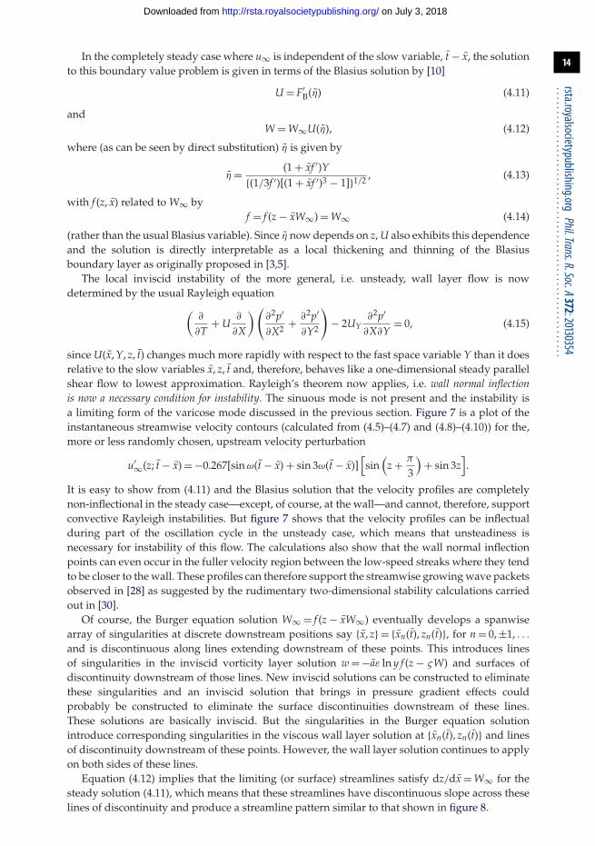
In the completely steady case where u∞ is independent of the slow variable, t − x, the solutionto this boundary value problem is given in terms of the Blasius solution by [10]

U = F′B(η) (4.11)

andW = W∞U(η), (4.12)

where (as can be seen by direct substitution) η is given by

η= (1 + xf ′)Y{(1/3f ′)[(1 + xf ′)3 − 1]}1/2 , (4.13)

with f (z, x) related to W∞ byf = f (z − xW∞) = W∞ (4.14)

(rather than the usual Blasius variable). Since η now depends on z, U also exhibits this dependenceand the solution is directly interpretable as a local thickening and thinning of the Blasiusboundary layer as originally proposed in [3,5].

The local inviscid instability of the more general, i.e. unsteady, wall layer flow is nowdetermined by the usual Rayleigh equation(

∂

∂T+ U

∂

∂X

)(∂2p′

∂X2 + ∂2p′

∂Y2

)− 2UY

∂2p′

∂X∂Y= 0, (4.15)

since U(x, Y, z, t) changes much more rapidly with respect to the fast space variable Y than it doesrelative to the slow variables x, z, t and, therefore, behaves like a one-dimensional steady parallelshear flow to lowest approximation. Rayleigh’s theorem now applies, i.e. wall normal inflectionis now a necessary condition for instability. The sinuous mode is not present and the instability isa limiting form of the varicose mode discussed in the previous section. Figure 7 is a plot of theinstantaneous streamwise velocity contours (calculated from (4.5)–(4.7) and (4.8)–(4.10)) for the,more or less randomly chosen, upstream velocity perturbation

u′∞(z; t − x) = −0.267[sinω(t − x) + sin 3ω(t − x)]

[sin

(z + π

3

)+ sin 3z

].

It is easy to show from (4.11) and the Blasius solution that the velocity profiles are completelynon-inflectional in the steady case—except, of course, at the wall—and cannot, therefore, supportconvective Rayleigh instabilities. But figure 7 shows that the velocity profiles can be inflectualduring part of the oscillation cycle in the unsteady case, which means that unsteadiness isnecessary for instability of this flow. The calculations also show that the wall normal inflectionpoints can even occur in the fuller velocity region between the low-speed streaks where they tendto be closer to the wall. These profiles can therefore support the streamwise growing wave packetsobserved in [28] as suggested by the rudimentary two-dimensional stability calculations carriedout in [30].

Of course, the Burger equation solution W∞ = f (z − xW∞) eventually develops a spanwisearray of singularities at discrete downstream positions say {x, z} = {xn(t), zn(t)}, for n = 0, ±1, . . .and is discontinuous along lines extending downstream of these points. This introduces linesof singularities in the inviscid vorticity layer solution w = −aε ln y f (z − ςW) and surfaces ofdiscontinuity downstream of those lines. New inviscid solutions can be constructed to eliminatethese singularities and an inviscid solution that brings in pressure gradient effects couldprobably be constructed to eliminate the surface discontinuities downstream of these lines.These solutions are basically inviscid. But the singularities in the Burger equation solutionintroduce corresponding singularities in the viscous wall layer solution at {xn(t), zn(t)} and linesof discontinuity downstream of these points. However, the wall layer solution continues to applyon both sides of these lines.

Equation (4.12) implies that the limiting (or surface) streamlines satisfy dz/dx = W∞ for thesteady solution (4.11), which means that these streamlines have discontinuous slope across theselines of discontinuity and produce a streamline pattern similar to that shown in figure 8.



15


.........................................................

0

–0.20

–0.50

1

2

3

4

5

6

7

–0.4 –0.3 –0.2 –0.1 0

–0.15

–0.10

–0.05

0

0.05

0

1

2

3

4

5

0.5 1.0x

x = 1.80

x = 1.57

x = 1.35

x = 1.12

x = 0.90

x = 0.67

x = 0.45

t = 5.4, x = 0.76

t = 6.26, x = 0.76

x = 1.80

x = 1.57

x = 1.35

x = 1.12

x = 0.90

x = 0.67

x = 0.45

U (x,Y, z, t )–F¢B

d2U /dh2 (h, z) = 2.13

h

0

1

2

3

4

5

6

7

h

z

1.5

0 –0.5 –0.4 –0.3 –0.2 –0.1 00.5 1.0x d2U /dh 2(h, z) = 2.13

1.5

–0.20

–0.15

–0.10

–0.05

0

0.05

0

1

2

3

4

5

z

U (x, Y, z, t ¯)–F¢B

Figure 7. Contours of constant streamwise velocity and its second derivatives at two different instants of time (calculated byDr Adrian sescu of Mississippi State University).

line of symmetry

Figure 8. Wall streamline pattern for Goldstein, Leib and Cowley problem [15].

This, in turn, suggests that there is a collisional separation along these lines ofdiscontinuity [32]. It can probably be thought of as a kind of bursting of the boundary layer that isusually associated with unsteady flows. This separation is of course steady, but the computationsin [30] show that similar but wholly unsteady types of separation occur when low-frequencyunsteadiness is added back into the upstream flow.

Numerical simulations of a similar type of flow in [33], which studies the impulsively startedflow produced by a spanwise-periodic array of vortices adjacent to a flat plate, show that theexpected eruptive separation (i.e. the formation of an eruptive spike) is prevented from occurring



16


.........................................................

by a localized instability in the cross flow motion when the Reynolds number is sufficiently high.Brinkman et al. claim that their extensive numerical computations prove that the instability isphysical and not numerical and present evidence to suggest that it is associated with Rayleighinstability of the spanwise velocity profiles as opposed to the streamwise profiles. However,Cowley [34] suggests that there may be some issues with these calculations and provides ananalytical argument that appears to show that this type of instability can arise spontaneously.

The experiments seem to show that the turbulent spots appear spontaneously without anyprecursor wave packets when the free-stream turbulence level is greater than 5% or so. TheBrinckman & Walker [33] instability is of the absolute or global type that grows in time ratherthan in space and appears to develop spontaneously in unsteady flows without external forcing.It may, therefore, explain the near spontaneous turbulent spot formation that occurs in theseexperiments [34]. This is of course fairly speculative and needs additional analysis before it canbe accepted as fact.

While the Nagarajan et al. [27] results imply that leading edge bluntness is extremely importantat the higher free-stream turbulence levels, Kendall [4] and Whatmuff [35] carried out someexperiments at relatively low free-stream turbulence levels which seem to show that changingthe leading edge aspect ratio changes the transition location but not the Klebanoff mode RMSamplitude and spacing. However, the turbulence was pretty low in their experiments and theirplates were fairly thin, and more importantly the screens were located upstream of a large windtunnel contraction in their experiments, which would tend to suppress the normal vorticityrelative to the streamwise component.

5. Summary and conclusionThere appears to be three somewhat distinct spot generation mechanisms that can occur whenthe free-stream turbulence level is greater than 1%:

(i) The breakdown of streak-like structures due to sinuous mode instability generated bydisturbances in the free stream. These streaks are primarily generated by streamwisevorticity in the upstream flow and appear relatively far downstream from the leadingedge whose exact geometry seems to be unimportant.

(ii) Breakdown of more vortex-like structures due to varicose mode instability. Thesestructures are primarily generated by plate normal vorticity in the upstream flow andappear to be concentrated near the leading edge [22]. The leading edge geometry seemsto play an important role here.

(iii) Instability arising from collision of vortex-like structures generated by plate normalvorticity.

It is also worth noting that the edge layer problem has largely been ‘swept under the rug’ in thispaper and further analysis of the flow in this region could turn out to be highly beneficial.

It is also worth noting that, while the focus of this paper has been on incompressible flows, theturbomachinery flows mentioned in §4c are highly compressible and could contain shock waves.The Klebanoff modes could also be strongly affected by acoustic disturbances emanating fromturbulent boundary layers. It may, therefore, be worth considering the effect of shock waves onthe Klebanoff modes, as recommended by one of the referees.

Acknowledgements. The author would like to thank Dr Adrian Sescu of Mississippi State University for carryingout the computations in figure 7.Funding statement. This work was supported by the NASA Aerosciences Project.

References1. Dryden HL. 1936 Air flow in the boundary layer near a plate. NACA Report no. 562. See

http://naca.central.cranfield.ac.uk/reports/1937/naca-report-562.pdf.


http://naca.central.cranfield.ac.uk/reports/1937/naca-report-562.pdf


17


.........................................................

2. Taylor GI. 1939 Some recent developments in the study of turbulence. In Proc. 5th Int. Congressfor Applied Mech. Cambridge, MA, 12–26 September 1938 (eds JP Den Hartog, H Peters), pp. 294–310. New York, NY: John Wiley & Sons, Inc.; London, UK: Chapman & Hall.

3. Klebanoff P. 1971 Effect of free stream turbulence on a laminar boundary layer. Bull. Am. Phys.Soc. 16, 203–216.

4. Kendall JM. 1991 Studies on laminar boundary-layer receptivity to free-stream turbulencenear a leading edge. In Boundary layer stability and transition to turbulence (eds DC Reda, HLReed, R Kobayshi), pp. 23–30. New York, NY: ASME.

5. Bradshaw P. 1965 The effect of wind-tunnel screens on nominally two dimensional boundarylayers. J. Fluid Mech. 22, 679–687. (doi:10.1017/S0022112065001064)

6. Crow SC. 1966 The spanwise perturbation of two-dimensional boundary layers. J. Fluid Mech.24, 153–164. (doi:10.1017/S0022112066000557)

7. Dong M, Wu Z. 2013 On the continuous spectra of the Orr-Sommerfeld/Squire equationsand the entrainment of free-stream vortical disturbances. J. Fluid Mech. 732, 616–659.(doi:10.1017/jfm.2013.421)

8. Wundrow DW, Goldstein ME. 2001 Effect on a laminar boundary layer of small amplitudestreamwise vorticity in the upstream flow. J. Fluid Mech. 426, 229–262. (doi:10.1017/S0022112000002354)

9. Goldstein ME. 1997 Response of the pre-transitional laminar boundary layer to free streamturbulence. Otto Laporte Lecture. Bull. Am. Phys. Soc. 42, 2150.

10. Goldstein ME, Wundrow DW. 1998 On the environmentally realizability of algebraicallygrowing disturbances and their relation to Klebanoff modes. Theor. Comput. Fluid Dyn. 10,171–186. (doi:10.1007/s001620050057)

11. Leib SJ, Wundrow DW, Goldstein ME. 1999 Effect of free stream turbulence and othervortical disturbances on a laminar boundary layer. J. Fluid Mech. 380, 169–203. (doi:10.1017/S0022112098003504)

12. Chu B, Kovasznay LSG. 1958 Non-linear interactions in a viscous and heat conductingcompressible gas. J. Fluid Mech. 3, 494–514. (doi:10.1017/S0022112058000148)

13. Goldstein ME. 1978 Unsteady vortical and entropic distortions of potential flows roundarbitrary obstacles. J. Fluid Mech. 89, 433–468. (doi:10.1017/S0022112078002682)

14. Hunt JCR, Carruthers DH. 1990 Rapid distortion theory and the ‘problems’ of turbulence.J. Fluid Mech. 212, 497–532. (doi:10.1017/S0022112090002075)

15. Goldstein ME, Leib SJ, Cowley SJ. 1992 Distortion of a flat-plate boundary layer by free-streamvorticity normal to the plate. J. Fluid Mech. 237, 231–260. (doi:10.1017/S0022112092003409)

16. Gulyaev AN, Kozlov VE, Kuznetson VR, Mineev BI, Sekundov AN. 1989 Interaction of alaminar boundary layer with external turbulence. Izv. Akad. Nauk SSSR Mekh. Zhid. Gaza 6,700–710.

17. Kemp NH. 1951 The laminar three-dimensional boundary layer and the study of the flow pasta side edge. MSc thesis, Cornell University, USA.

18. Ricco P, Luo J, Wu X. 2011 Evolution of instability of unsteady nonlinear streaks generated byfree-stream vortical disturbances. J. Fluid Mech. 677, 1–38. (doi:10.1017/jfm.2011.41)

19. Chandrasekhar S. 1950 The theory of axisymmetric turbulence. Phil. Trans. R. Soc. Lond. A 242,557–577. (doi:10.1098/rsta.1950.0010)

20. Simmons LFG, Salter MA. 1934 Experimental investigation of the velocity variations inturbulent flow. Proc. R. Soc. Lond. A 145, 212–234. (doi:10.1098/rspa.1934.0091)

21. Hall P, Horseman NJ. 1991 The linear inviscid secondary instability of longitudinal vortexstructures in boundary layers. J. Fluid Mech. 232, 357–375. (doi:10.1017/S0022112091003725)

22. Vaughn NJ, Zaki TA. 2011 Stability of zero-pressure-gradient boundary layer distorted byunsteady Klebanoff streaks. J. Fluid Mech. 681, 116–153. (doi:10.1017/jfm.2011.177)

23. Cowley SJ. 1985 High frequency Rayleigh instability of stoked layers. In Stability of timedependent and spatially varying flows (eds DL Dwoyer, MI Hussaini), pp. 261–275. Berlin,Germany: Springer.

24. Wu X. 1992 The nonlinear evolution of high-frequency resonant-triad waves in anoscillatory Stokes layer at high Reynolds number. J. Fluid Mech. 245, 553–597. (doi:10.1017/S0022112092000582)

25. Wu X, Choudhari M. 2003 Linear and nonlinear instabilities of a Blasius boundary layerperturbed streamwise vortices, Part 2. Intermittent instability induced by long wavelengthKlebanoff modes. J. Fluid Mech. 483, 249–286. (doi:10.1017/S0022112003004221)


http://dx.doi.org/doi:10.1017/S0022112065001064


http://dx.doi.org/doi:10.1017/jfm.2013.421



http://dx.doi.org/doi:10.1007/s001620050057








http://dx.doi.org/doi:10.1098/rsta.1950.0010

http://dx.doi.org/doi:10.1098/rspa.1934.0091







18


.........................................................

26. Swearingen JD, Blackwelder RF. 1987 The growth and breakdown of streamwise vortices inthe presence of a wall. J. Fluid Mech. 182, 255–290. (doi:10.1017/S0022112087002337)

27. Wu X. 1995 Generation of Tollmien-Schlichting waves by convecting gusts interacting withsound. J. Fluid Mech. 397, 285–316. (doi:10.1017/S0022112099006114)

28. Nagarajan S, Lele SK, Ferziger JH. 2007 Leading-edge effects in bypass transition. J. FluidMech. 572, 471–504. (doi:10.1017/S0022112006001893)

29. Toomre A. 1960 The viscous secondary flow ahead of an infinite cylinder in a uniform parallelshear flow. J. Fluid Mech. 7, 145–155. (doi:10.1017/S0022112060000098)

30. Goldstein ME, Sescu A. 2008 Boundary layer transition at high free-stream disturbancelevels—beyond Klebanoff modes. J. Fluid Mech. 613, 95–124. (doi:10.1017/S0022112008003078)

31. Atassi HM, Grzedzinski J. 1989 Unsteady disturbances of streaming motions around bodies.J. Fluid Mech. 209, 385–403. (doi:10.1017/S0022112089003150)

32. Lighthill MJ. 1963 Boundary layer theory. In Laminar boundary layers (ed. L Rosenhead), p. 74.Oxford, UK: Oxford University Press.

33. Brinkman KW, Walker JDA. 2001 Instability in a viscous flow driven by streamwise vortices.J. Fluid Mech. 432, 127–166.

34. Cowley SJ. 2001 Laminar boundary-layer theory: a 20th century paradox? In Proc. ICTAM2000, Chicago IL, 27 August–2 September 2000 (eds H Aref, JW Phillips), pp. 389–411. Dordrecht,The Netherlands: Kluwer.

35. Whatmuff J. 1998 Detrimental effects of almost immeasurably small freestreamnonuniformities generated by wind-tunnel screens. AIAA J. 36, 379–386.









effectoffree-stream turbulenceonboundarylayer...

Documents