9, 6

DNA-TR-86-243-V5

EFFECTS FOR ICBM BASINGVolume V-Row Field Modeling

Q, David P. Bacon IneaonlCo.oato.. "Science ApplicAtions Interationl CorporaionP. O. Box 1303 3.

7 McLean, VA 22102-1303

~ 31 December 1985

Technical Report

CONTRACT No. DNA 00184-C-0130

THIS WORK WAS SPONSORED BY THE DEFENSE NUCLEAR AGENCYUNDER RDT&E RMSS CODE 334406446 YV XSO0021 H25900.

DTICPrepared for EL ECTEDirector NOV 27.198

DEFENSE NUCLEAR AGENCYWashington, DC 20305-1000 U

L. 8i 113

UNCLASSIFIEDSECURITY CLASSIFICATION OF THIS PAGE

REPORT DOCUMENTATION PAGE 00110 o 0011,11111

Ia. REPORT SECURITY CLASSIFICATIONE 1b RESTRICTIVE MARICIGS,UNCLASSIFIED ________________________

2a. ECIURiTY CLASSIFICATION AUTHORITY JI.DISTRIBUTION/AVAILITY OF REPORTN/A since Unclassifiled

2b. DECLASSIFICATIOIN I OWNGRAOING SCHEDULEN/A sinceUnclassified______________________

4. PERFORMING ORGANIZATION REPORT NUMBERS) S. MONITORIN ORGANIZTION IEPORT NUMSERCS)

SAIC 85/1742 D1%-T-86-243-V5

66. NAME OF PERFORMING ORGANIZATION 6b. OFFICE SYMBOL 7a. NAME OF MONITORING ORGANIZATIONScience Applications Of a~ka* DirectorInternational Corporation Defense Nuclear Agency

6C. ADDRESS (0y SW. &W ZI WC) 7b. AOMRSS (CIy. Ste W. ZIP WC0*I

P. 0. Box 1303 Washington. DC 20305-1000McLean, VA 22102-1303

4a. NAME OF FUNDIN4GI SPONSORING 111. OFFICE SYMBOL 9. PROCUREMENT INSTRUMENT IDENTIFICATION NUMBER

DNA 001-84-C-0130

IL. ADDRESS (Cie Staff WW ZP CC) 10 SOURCE OF FUNDING NUMBERS IOKUIPROGRAM RJC ITS WOKUIELEMENT WO INPOJC ITNASCESIKEN

____________________________ 62715R I 99wIs G DZ0021211. TITLE Ondaf S OainC~ftOWV

EFFECTS OF IC(BASINGVoluim V-Flow Field mdeling

12. PERSONAL AUThOR(S)"acon 0 David P.

13e. TYPE OF REPORT 13b. TIME COVERED 1I. DATE OF REPORT (Vw.r MwRoviA") 15 S PAGE COUNTTechnical PFROMl2 & 33 3 ~ n i 851231

16. SUPPLEMENTARY NOTATIONThis work was sponsored by the Defense Nuclear Agency uner UDTAE NSS Code 3344084466"9(NMG00021 12590D.

17. COSATI CODES. It SUBJECT TERMS (CaftnWi an mvwwu if amamvy and i*Mo by blck mRibsrJFIELD GROUP SUs-GR0QP meteorology

3 Nuclear Weapons Effects16M 1 - I Nuclear Winter

19. ABSTRACT (Con~nus on ,svinv if ninCMuvY OWd i*0 by Backn AWI&Vdr

The effect of the amient meteorology (temerature and davpoint profiles) on thedyemeics of a rising fireball and the plusm from a large-area fire (f irestorm) has beenstudied. The primary results indicate the Importance of mlsture for both phenomena andIndicates that the amient meteorology amy grossly affect cloud stabilization and pre-cipitation. The role of precipitation and Its resultant scavenging remains to be inves-tigated.

20 DISTRIBUTION I AVAILABIUITY OF ABSTRACT 121 ABSTRACT SECURITY CLASSIFICATIONU UNCLASSIPIEOUNLIMITIED n LAME AS MPT C VTIC USERS IUNCLASSIFIED

12a NAME OF RESPONSIBLE INDIVIlDUAL 22b. TELEPHONE (Miakds AfsoC111) 22C.of FICESYMNOLBetty L. Fox (202) 325-7042 1DNA/S171

DO FORM 1473.34 MAR 83 APR osmoA im be used uftil 01"W SECURITY CLASSIFICATION OF THIS5 PAGEAU O~dto atanmobgsolew UNCLASSIFIED

i

1UECLASSIIIUSECURIT CLASSIPIATKIUW PI FN AUK

SECU.?, c.LIIA~o. THIS PAGE

UICLASSUIED

±1

EXECUTIVE SUMMARY

In an attempt to bring a new capability to the problem of nuclear fireball rise

and the dynamics of the plumes from nuclear-burst induced firestorms, a joint program

of SAIC and NASA/LaRC and their contractor Systems and Applied Sciences Corpora-

tion (SASC) was launched. This program centered on modifying and applying the

Terminal Area Simulation System (TASS) to the above problems. The result of this

effort is a new research tool for use in the study of nuclear weapons effects problems.

TASS was used to study the effects of the ambient meteorology (temperature

and dewpoint profiles) on the dynamics of both rising fireballs and the plume from a

large area fire or firestorm. In addition, it was used to investigate the effect of thespatial distribution and time history of the fire on the dynamics and the stabilization

of the resulting cloud. The preliminary results Indicate that the cloud stabilization is

not sensitive to either the spatial distribution of the fire or to its time history, but

rather is interested in the total energy Input to the atmosphere by the fire. On the

other hand, the stabilization is strongly dependent on the ambient meteorology,

especially the amount of moisture present.

Even though we have not exhausted the study of the effect of the ambient

meteorology, we have identified two new areas of research that may also be

important: three-dimensional effects and the effect of scavenging of particulates by

precipitation. These research areas should constitute the core of a continuing

program.

A0essto0 For

D TC TAB

Ujn o.ced 0just Lf Le~t 1o----

Distriutpon/Av.ailabt]lity C CKeS___.

Sspecialill DID,,t

•~~~~~~~~~~~~~~ .011 •IIII I•III II IIII

CONVERSION TABLE

Cuiefame for U-S. Cuomuy w mtum (SI) sawi of umuuums

MULTIPLY BY --- W TO GETTO GIFT ' Y 04 DIVIDE

arm 1. use. ONXI .10 .....immeow r emiI3 OS3 86 X t 2 b pfiftm (19*

erm"*inal wl lamseeanmu 1. 416 2N X 3.*3 bo IIWomn lamuselI 4.10 Oft M a gm01on slammmell"" 4.184 so XE 92 wep Iiaft/m2 flu/*,)We 3 "SO X13 I1 Im bemml fewa

delm 4411611) 1. 1"4anx a 4 "AM 49I*6166 Fabs04'. Not* 4041. da boo" Wm flu

*No m 1s . 11 06 X X E -ombIS

(mm4se. 1. 31 Ili bob Wplim IV S. awgud 3. M5141 3 4mr 1A2.

OnWailrfm IJAigesaau wmd

bihama 4.Um tm-141W~i411441 a ...amu.3 mont

1,4 S041111z.2xela

mawm I m wx 6 mva

adl Imnuamla 2.1 4 go~ 111si aderetu A. Ift364XE. 9 3 10140 m)

pwW-fre sIb. ateiupu 4.40=2 gam IN

paw~e/lmsI sp em 1.2 . imusmifice (11/w

ea-ifmimes Irm stnmopeal 4. 11104 xE9 .1 mks-rm Ik

psinanmso aaa 0 1 1dooi

"A .iaam 4bua. Lead m em 13 a ~ -8 00M4"s"m M 11 a 2-4 A

A 41N X9-6 ellea)1.q 2.531 2-I leftnaibw

Wi wtn. q*C) 1.3223 XE-I 41 11111,a fkw1b . -msey "@-I Ift o.Uunf r~mgsvssl; a lk. I ofwt/s.

*Tb. Cray CIO a *a I ns og 0..r~a

iv

TABLE OF CONTENTS

s don LPap

EXECUTIVE SUMMARY - i

CONVERSION TABLE IV

LIST OF ILLUSTRATIONS vi

LIST OF TABLES vu

I INTRODUCTION 1

2 THE TERMINAL AREA SIMULATION SYSTEM (TASS) 3

3 FIREBALL SIMULATIONS 9

4 LARGE-AREA FIRE SIMULATIONS II

3 CONCLUSIONS 21

TYPICAL TASS DIAGNOSTIC OUTPUT 23

V

LIST OF niLUSTRATIONS

Figwe Pape

1 Test of boundary condition using 30 x 30 km domain (top) and1. x 1 km domain (bottom)

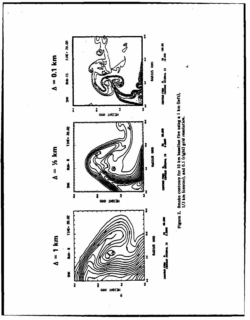
2 Smoke contours for 10 km baseline fire using a I km (eft),1/3 km (center), and 0.1 (right) grid resolution 6

3 Rise of a I00oC thermal bubble (fireball) in two differentsoundings: a dry mafa, TX case (left) and a wet Lake Charles,LA case (right) 10

4 Baseline large area fire simulation - smoke contours 13

5 Comparison of smoke contours for baseline simulation (left) andannular fire (right) 15

6 Comparison of smoke contours for baseline simulation (left) andfast burn/smoldering fire (right) 16

7 Comparison of smoke for baseline simulation (left) and dryatmosphere simulation (right) is

a Comparison of smoke contours for 4 fires: a 2 km triggering fire(top left) a 6 km trigering fire (bottom right) a 2 km I hourfire (top right) and a[0 km triggering fire Uottom left) 19

9 Relative humidity (%) 24

10 Radial velocity (m/s) 23

11 Vertical velocity (m/s) 26

12 Temperature deviation (oC) 27

13 Streamlines 25

14 Pressure deviation (mb) 29

1S Rain (gjkg) 30

16 Hail (g/kg) 31

17 Total precipitation 32

18 Radar reflectivity 33

19 Equivalent potential temperature (K) 34

20 Massless tracer 35

vi

LIST OF TABLES

Table Page

1 The terminal area simulation system (TASS)

2 TASS grid resolution test cases 7

3 Summary of TASS firestorm calculations 12

t'2 .,4 die*4 4y .

SECTION 1

mmooucnom

In the past, the calculation of fireball rise has been performed witil one of two

classes of code: phenomenological or first-principles shock/hydrodynamic. The

former was fixed to the DNA I KT standard and then scaled In various ways; the latter

attempted to resolve the shock physics for the developing fireball and then followed

the buoyant rise thereof. Neither approach is acceptable. The former can be shown toyield numbers of little use to investigators requiring detailed information on thefireball, and the latter requires an Inordinately large amount of computer time to

study the late-time (-1 min) fireball rise.

The primary problems with employing a shock/hydrodynamic code to thephenomenon of fireball rise are three: (1) once the shock has propagated out of the

computational domain (T of the order of 100 sec), the high resolution of the shock codeis not needed and serves as a huge computational overhead (even before this time theshock has decayed sufficiently to be treated as an acoustic wave and shock resolution

is not strictly necessary) (2) most shock/hydro codes are Inviscid and while thisapproximation Is valid during the period that the shock physics dominates, the fireballrise problem depends a great deal on the turbulence and entrainment processes and

therefore on the viscosity; (3) none of the shock hydrocodes to date has considered the

effect of the meteorology (temperature and dewpoint profile) on the fireball rise.

In an attempt to circumvent the above problems, SAIC, in collaboration with

NASA/ILaRC and their contractor Systems and Applied Sciences Corporation (SASC),has been working to modify a non-hydrostatic meteorological code, the Terminal AreaSimulation System (TASS) to allow for the study of nuclear fireball rise and the study

of the dynamics of plumes from large area fires and firestorms. The reason that such

a code was deemed suitable for these problems is that as a non-hydrostatic code, itretains the acoustic pressure waves and therefore while it is not capable of capturing

and retaining a shock wave, after approximately 30 seconds, the shock from a nuclear

cloud is traveling at the speed of sound and is weak enouh to be considered to be asimple acoustic wave. In addition, since TASS is a meteorological code, it has

inherently in it the cloud microphysics and hydrometeor formation and growth

I

processes that are significant if one wants to understand the water and ice problem.

The fact that this-Is a much more efficient algorithm allows us to investigate many

more scenarios than is possible with a shock/hydro code.

During the past year, SAIC performed a large number of simulations of rising

fireballs and the plumes from large area fires. In this report we will document a few

of the calculations performed. First, however, we present a brief synopsis of TASSand some of the validation studies performed on It.

2

SECTION 2

THE TERMINAL AREA SIMULATION SYSTEM (TASS)

The Terminal Area Simulation System (TASS) is a non-hydrostatic computer code

originally developed by Fred Proctor of SASC to model the development of strongisolated convective activity. The code contains parameterizations for the formation

and size distribution of both precipitating and non-precipltating hydrometeors: rain,hail, snow and cloud water and Ice. This parameterization includes the release of the

latent heat of condensation and solidification as well as the main interactions betweenthe various classes of hydrometeors. Table k contains an overview of the basic

features of the code.

Various tests have been performed to see the effect of the grid size and the

boundary conditions on the simulations to be reported below. Figure I shows the

effect of the boundary conditions on the simulations reported. The top figure showsthe smoke contours at 20 minutes into a large area fire simulation run over a 30 km x

30 km domain with a 1/3 km grid resolution; the bottom figure represents the same

simulation run over a 1 km x 13 km domain. This fIgure very nicely shows the lack of

interaction with the lateral boundary.

In a similar vein, Figure 2 shows a comparison of the same simulation as above

run with grid resolutions of 0.1, 1/3, and I km. Because of the differing contour

levels, one must look at particular concentration contours in order to evaluate the

differences between the three simulations. Table 2 shows an evaluation of two

different contour levels.

3

Table 1. The terminal area simulation system (TASS).

Prognostic Equations for: MomentumPressurePotential TemperatureWater VaporCloud WaterCloud IceRainSnowHailSmoke (Massless Tracer)

Turbulence Closure: Smagorinsky - depends on stratification and shear

Boundary Conditions: Surface - Nonslip velocity- Continuous thermodynamics- Time-dependent surface heat source

Axial - Symmetric for all variables

Lateral - Open boundary for all variablesRadiative wave speeds from interior points

Top - Zero vertical velocityConstant potential temperatureAll other variables continuous

Parameterizations: Autoconversion of cloud water Into rainAccretion of cloud water by rainEvaporation of rainSpontaneous freezing of supercooled cloud water and

rainInitiation of cloud iceAccretion of cloud water by cloud IceAutoconversion of cloud Ice Into hallDeposition and sublimination of hail and cloud iceAccretion of cloud water and cloud Ice by hailFreezing of rain due to the collision of cloud ice and

supercooled rainShedding of unfrozen water by hailInitiation of snowAccretion of cloud water by snowMelting qf cloud ice, snow, and hail

Additional Diagnostics: Radar reflectivityHydrometeor concentrations

4

SMK RUN- 4 TIME= 20.02

agN oloeJg .uu...uuelu. gjuph ouuu op# o os f "Iu p off , Inui IIu I eofIIIalInIgoIuIuI

use

.

9 . al Ilu ....

..................

Figure 1. Test of boundary conditions using 30 z 30 km domain (top) andI5 z 15 km domain (bottom).

cs tc2

E A

3 3 as

20

.

amEM36£

Table 2. TASS grid resolution test cases.

Grid Size (kin) Maximum Height of Contour (km)

13 300.1 11.5 10. -

0.3 12.0 11.71.0 1#.0 13.0

Thus we see that Increasing the grid size by a factor of 10 results in only a 25%

Increase in the maximum altitude of the smoke tracers in these simulations. Since the

computation time Increases with the number of computational cells, for our productionruns we used a 1.0 km grid cell; for special runs, we employed a 0.5 km grid cell.

One other point should be noted in Figure 2 and Table 2s the region of non-

agreement between the different cases Is mostly near the axis. This is because anycode with axial symmetry has a problem handling diffusion and entrainment at the

axis. This is one of the reasons why we felt that we needed to expand the code tothree-dimensions, a process which Is ongoing at NASA.

In Appendix A we include a complete set of the diagnostics produced by TASS at

one point in time for one of the large-area fire simulations described in Section IV

below. This set Includes: the relative humidity (%), RLH; the radial, U, and vertical,w, velocities (m/s); the temperature deviation (oC); the streamlines, PSI; the pressure

deviation, P; the rain, XIP, hal, XIH, and total, XIT, precipitation (g/kg); the radarreflectivity, RRF; the equivalent potential temperature, EPOT; and the massless

tracer, SMK.

mm mmmmmmmm mm mmmm m 7

S

8

SECTION 3

FIREBALL SMULATIONS

Early in the contract period, two simulations of a fireball rise were performed;

one using a sounding from Maria, TX, the other a sounding taken 3 hours later in Lake

Charles, LA. The Maria sounding was dry and had a tropopause at approximately

11.0 km while the Lake Charles sounding was very wet (with 1.63" of precipitablewater vapor) and had a tropopause at approximately 13.5 km. The two simulations

were Initiated by adding a thermal "bubble" of overtemperature at the surface. The

bubble was hemispherical and had a peak overtemperature of 100 0 C and was intendedto represent the thermal energy of a nuclear burst of yield 0(1 MT). Figure 3 shows

the relative humidity profiles from these simulations. (These simulations were run

with a 0.5 km grid size.) As can be seen, the visible cloud (represented by the 100%

relative humidity - the Innermost contour) at 3 minutes Is 3.5 an higher in the wet

sounding than in the dry sounding. Part of this difference may be due to the differentlevels of the tropopause, but part of It Is due to the release of the latent heats of

condensation and fusion.

9

MIR4A

100

*0

2~ -p

4~I ddt

UU

1' 10

SECTION 4

LARGE-AREA FIRE SIMULATIONS

A large number of simulations were performed on the response of-the atmos-

phere to a perturbation resembling that of a large area fire. These simulations used a

I km grid size and were performed for a variety of fire Intensities, sizes, spatial

distributions, time histories and for a variety of atmospheric soundings. Since so many

cases have been run, we have selected just a few to discuss in detail. In Table 3 we

present an overview of the results of many of the simulations.

Case I (Designated Run-O) This was our baseline case. The atmospheric

sounding is the same Lake Charles sounding mentioned above and Is a moist, unstable

atmosphere. The fire was a uniform 10 km radius which started cold at time T=O and

rose linearly in time to a peak power density of 0.23 MW/m 2 (for a total power input

of roughly 8 x 1013 W) In 15 minutes. The fire maintained this intensity for 30 minutes

and then linearly decayed to zero in 13 minutes. Thus at 1 hour Into the simulation,

the fire was out. Over Its I hour duration, the fire provided 2 x to'1 3 (which is

equivalent to 30 MT) of thermal energy.

In Figure 4, we show the smoke tracer for. this fire at times 10, 30, 30, and 70

minutes. At 10 minutes nto the simulation, the fire has not reached its peak intensity

and the smoke Is confined to a disk shaped region approximately 4 km in height by

10 km In radius. By 30 minutes into the simulation, the smoke plume has reached an

altitude of 23 km and a radius of 33 km. Three factors have caused this rapid growth

in the plume: (1) the fire heat source achieved its maximum intensity at T=13 minutes

and has been providing a trong thermal input; (2) the moisture lofted by the addition

of heat reached the saturation point and condensed providing an additional thermal

Input due to the release of latent heat; and (3) the upwelling air mass has associated

with It a strong radial outflow at altitude (and a radial inflow near the surface) which

carries the smoke with It. Other than "filling in", little change occurs in the cloud

over the next 20 minutes. The fire Is beginning Its decay phase but is still supplying a

considerable amount of heat and smoke to the atmosphere. By 70 minutes, with thefire now out, the plume begins to decay with the smoke forming a band between 9 and

21 km.

11

aU0C -c - -

N - - N N N - N ~ml S S

- - -

so

jCC N0%a N-eN

a'I2b.04d i.

Is

- 9.- 246 1.2

'3'

2 -

'I -

5 5.- 2- - gA k

I-s I-s I-F- ~I.

.1 '~ 4' ' zj~_ z

-~ - so* N~ W%

* II I U,

soI ii C2 2ED 6

12

SIP AIM- 0 ripts 10.00SI ft-O a I,( 30.00

S.. - . . . .. . . . . . . . .m

RAIU 00 RDUSa

.4 *A " o s s* s s S .

RADIUS No0 RADIUS am0

1~ 1

Case 2 (Run-l) This case Is the most extreme of the cases run varying the fire

spatial distribution" (MW/m 2) while keeping the total power (MW) the same. The fire

was uniform, but over an annulus from 6 to 10 km. The time history (15 minute rise,

30 minute plateau, 13 minute decay) was the same, however, in order to keep the same

total power, the peak intensity was increased from 0.25 to 0.39 MW/m 2 . At might be

expected, the early and mid-time smoke plumes show a considerable change from our

baseline case. This Is due in part to the early formation of a downward flow on axis

which takes some time to overcome. The post-fire plume, however, is remarkably

similar to the baseline case with the smoke stabilizing In a 9-19 Ia band. FigureS

compares the 10 and 70 minute smoke contours for the uniform and annular fires. In

all four simulation Investigations the effect of the spatial distribution, the post-fire

smoke stabilized within a band from 9-21 km.

Case 3 (Run-100: This case explored the effect of varying the fire time history

while keeping the same total energy input (30 MT thermal). We reverted to our

baseline fire spatial distribution (uniform, 10 km radius) but the fire time history

consisted of a "fast burn" followed by a "smoldering fire". This fire ramped in 32 2minutes to 0.075 MW/m and then in the next 3 minutes climbed to 0.73 MW/m . This

intensity remained for 5 minutes followed by a decay to 0.13 MW/m 2 over the

following 5 minutes. The fire then decayed to zero over the next #0 minutes.

This simulation has some striking features. At 10 minutes, even though the fire

has reached its peak intensity, the atmosphere has not had time to respond; in

addition, the "bow wave" of the air above the axis has a strong resistance to the rising

air mass. (This may be caused by the forced axial symmetry of the simulation.)

However, a look at the comparison presented In Figure 6 shows that by 30 minutes the

intense fire period has served to loft smoke to an altitude of 30 km where the baseline

peak altitude was 25 km. (This increase may also be a figment of the forcedaxisymmetry which reduces the entrainment on axis.) This shows the sensitivity over

short periods of time of the plume to the total fire intensity. A look at the smoke at70 minutes on the other hand shows that it has stabilized in a band from 9-20 km, the

same band as the baseline study. This indicates that while the short-time atmospheric

response may depend on the fire intensity, the long time response is only a function of

the total thermal energy input.

14

sinc( .urs- 0 ris[. I0.00 S.m ru- I r[c. I0.00

33l. 5r~.•.. ... ..

O S I06 SO

IAOIuI Oft awul 0O

INSISON- SO T.. O Of I ft, d O.Oq

14 Sis

-- ]

Sdanua frS(ldh)

15

Nw um- 0 floes 30.00 fto-100 TIES, 30.o

r 4

-- - - -- - -- - - -

SO M A & ad 1 AG " " as a .

RAIIS00 ua 0

4wa4.

SA

AMaU ovmaOSa

Fiue6 Omtlaofsoecnor o aslnsiuaon(etad

fatbrnsodrigfr (ih)

16

This last observation may be due in part to the fact that we are overdriving the

atmosphere to the point that the cloud dynamics are being driven by the latent heat

release. During these simulations, more energy was released due to condensation and

solidification than was input by the fire; in addition the latent heat release occurred

where it would have the most impact on the smoke lofting - in the cloud itself.

Case 4 (Run-900): In order to explore the effect of the latent heat release, we

repeated the baseline case with the same Lake Charles temperature profile but with

no moisture. Figure 7 shows a side-by-side comparison of the baseline fire with (left)

and without (right) moisture. As Is obvious, the moisture content of the atmosphere

plays a crucial role in the cloud dynamics. For this reason, the use of a standard (dry)

atmosphere for these type of calculations should be avoided.

Trhlmerina Cases: As a finak series of simulations, we explored the amount of

energy required to "trigger" convective activity for the unstable Lake Charles

sounding. Figure 8 shows the 70 minute smoke clouds for four different fire space and

time distributions. The upper left plot shows the smoke contours resulting from a

2 km radius "triggering" fire. (A triggering" fire turns on at time T=I0 minutes,

peaks at TzI minutes, and ends at Tz20 minutes.) This fire deposits 223 kT of

(thermal) energy into the atmosphere. Compare this case to the two cases shown on

the right hand side of Figure As the upper plot shows the 70 minute smoke from a 2 km

radius fire with the full baseline 0l hour duration) time history; the lower plot shows

the mode from a 6 km radius fire with a "triggering" time history. Each of these cases

deposits 2 MT of energy. The final case shown (lower left) is a 10 km radius

"triggering" fire which deposits roughly 3.6 MT of energy into the atmosphere.

The signficance of thee runs Is that they span a factor of 20 in Input energy and

yet in all cases the smoke reached the tropopause. This is good evidence that more

attention needs to be paid to the ambient meteorology in this type of simulation.

17

rl- 0 TIIE, 10.00 Sa' TiI-OE Sr. 10.0

a.. . __ __.6_:

ilAOllJS OcO11OU004

SM MAI- 0 IME@R, 7.01 lMA-cJO0 rt1W .0.

4

04 a4

II01I. 5.4lg ((M

I I i

i4 04

i4 I

SO asaJAasa 4a

Figlure 7. Comparison of smoke for baselne simulation (left) anddry atmosphere simulation (right).

'a18

a -. 04 mmm m mm m

SI6 ZZSKT LCH N INJOWI TIMIC.70 uSC " ?.MLC K IRE1

*A 3

A, .A$,..

XM4U 0"RDISO

pOur S.Cmaio fsoecnor or ie:a2k tigrIgfr

(to let) a4 64 km trgern fir (boto rigt) a 2 km I hou f.ire

(t-o right) 70.a 0 km trigerin fire (bto left).

3* . -. 19

Conclusions. The major conclusions that we have drawn from this series ofsimulations are:

(1) The ambient meteorology plays a dominant role in the atmosphericresponse.

(2) Given Identical source total power, independent of spatial distribution (atleast over a 10 km scale size area), the atmospheric response will besimilar.

(3) The ambient moisture Is a key parameter - Its presence allows the cloudto equillbriate at and above the tropopause; its absence results In a verylow (sub-tropopause) stabilization height.

(4) Scavenging physics must be considerably Improved. Total condensation can

exceed 1014 g; total precipitation can surpass 109 g.

20

mmmmemm mmm mmn nmmnmaimnmn um nm nto amMai

SECTIONSCONCLUSIONS

The overall conclusions which we draw from our simulations of the atmospheric

response to both rising thermal bubbles (fireballs) and large area heat sources (large

area fires) are:

(1) Considerably more work must be done to investigate the role of the

ambient meteorology in understanding bott fireball rise and the atmospher-

Ic response to large-area fires.

(2) The details of the ambient sounding over and above the simple analysis of

the altitude of the tropopause do affect the cloud dynamics.

(3) The water vapor plays a very Important role In the cloud dynamics.Without it, the plume from a large-area fire does not reach the tropopause;with It, a significant amount of precipitation occurs which may result insome level of scavenging of any injected particulates.

In addition to the above conclusions, we have identified certain areas of further

research:

(1) Three-dimensional simulations. In both fireball rise and the cloud dynamicsof large-area fires, the effect of wind shear needs to be Identified. In the

case of the large-area fires, the effect of the winds may increase the

altitude of injection if the additional entrainment caused by the winds is

less than the damping the flow currently feels due to the precipitationoccurring over the heat source.

(2) Scavenging. The large amount of precipitation which we observe in our

simulations of both the fireball rise and large-area fires may provide a

great deal of scavenging of particulates.

These research areas are among those undergoing current study.

21 PAS 7.7 4