EFFECTS OF FEATURE TRANSFORMATION AND SELECTION ON CLASSIFICATION OF

NETWORK TRAFFIC ACTIVITIES

LIM WEN YING

FACULTY OF COMPUTING AND INFORMATICS

UNIVERSITI MALAYSIA SABAH

2015

EFFECTS OF FEATURE TRANSFORMATION

AND SELECTION ON CLASSIFICATION OF

NETWORK TRAFFIC ACTIVITIES

LIM WEN YING

THESIS SUBMITTED IN PARTIAL FULFILMENT FOR THE BACHELOR OF COMPUTER SCIENCE

(NETWORK ENGINEERING)

FACULTY OF COMPUTING AND INFORMATICS

UNIVERSITI MALAYSIA SABAH

2015

ii

DECLARATION

I hereby declare that this thesis, submitted to Universiti Malaysia Sabah as

partial fulfilment of the requirements for the degree of Bachelor of Computer

Science (Network Engineering), has not been submitted to any other

university for any degree. I also certify that the work described herein is

entirely my own, except for quotations and summaries sources of which have

been duly acknowledged.

This thesis may be made available within the university library and may

be photocopied or loaned to other libraries for the purposes of consultation.

22 JUNE 2015 …………………………………

LIM WEN YING

BK 1111 0156

CERTIFIED BY

_________________________________

Dr. Mohd Hanafi Ahmad Hijazi

SUPERVISOR

iii

ACKNOWLEDGEMENT

First and foremost, I am grateful to God for the good health and well-being

that were necessary to complete this research paper. I must thank my parents and

family for their understanding and support. They have always given their kindness,

patience and tolerance when I had rough times.

I wish to express my utmost appreciation and deepest gratitude to my

supervisor, Dr Mohd Hanafi Ahmad Hijazi. He constantly provided me with

constructive comments for improvement to this project. Weeks after weeks and

consultations after consultations, he continuously enlightened me when I was in

doubt and when there were areas that I lacked knowledge. In addition, he always

gave words of wisdom that encouraged me to continuous work on this project.

Without his continuous dedication in guiding me, I would never have completed this

research paper.

Last but not least, Associate Professor Dr Rayner Alfred who provided me

advice on improving the quality of this research paper for which I am thankful to. I

also place on record, my gratitude to one and all, who directly or indirectly, have lent

their hand in this venture.

LIM WEN YING

22 JUNE 2015

iv

ABSTRACT

As new technologies are emerging day by day, network, regardless of the Internet or Intranet within a corporation often plays a crucial role in connecting people from all around the world. From military use to achieving business goals and household need, data security often get attention from computer scientists. Traditional security measures that include the installation of firewall and antivirus software are commonly utilised to prevent intrusion. However, such types of defence are merely sufficient to secure a network and data travelling across it. Thus, second lines of defence like Intrusion Detection System (IDS) and Intrusion Prevention System (IPS) are introduced to overcome the inadequacy of traditional security measures. Generally, IDS uses two approaches, the Anomaly Detection (A-IDS) and the Misuse Detection in order to identify patterns of intrusion. A-IDS often perform comparison of the model of normal and anomalous model. Depending on the ability to measure similarity or distance between a target and a known type, comparison is made to determine whether to establish a new target anomalous or not. This research aims to investigate the effects of feature transformation on the classification of network activities; the focus is to represent the data into point series form to permit the application of Time Series Classification (TSC). The TSC technique used is k-Nearest Neighbour (KNN) coupled with Dynamic Time Warping. Effects of using different similarity measures, Euclidean Distance (ED) and Cosine similarity algorithm are also investigated. Experiments conducted involve conversion of the categorical data by three different conversion techniques to generate point series data – simple, probability and entropy conversion. Comparison between different classifiers is also conducted. The performance of the classifier is best using 1NN with Euclidean distance and entropy conversion for categorical data, where the recorded accuracy is 99.19%.

v

ABSTRACK

Pembaharuan teknologi berlaku setiap hari, rangkaian, tidak kira daripada Internet mahupun Intranet yang terdapat dalam sebuah korperasi sering memainkan peranan penting dalam menghubungkan orang ramai dari seluruh dunia. Daripada penggunaan oleh pihak tentera atau dalam bidang perniagaan untuk mencapai matlamat harian dan keperluan isi rumah, keselamatan untuk data yang mengalir di seluruh rangkaian sering mendapat perhatian daripada ahli-ahli sains komputer. Langkah keselamatan tradisional termasuk pemasangan “firewall” dan perisian antivirus biasanya menggunakan untuk mencegah pencerobohan. Walau bagaimanapun, jenis pertahanan tersebut semata-mata adalah tidak cukup untuk memastikan keselamatan rangkaian dan data yang merentasinya. Oleh itu, pertahanan peringkat kedua seperti “Intrusion Detection System (IDS)” dan “Intrusion Prevention System (IPS)” diperkenalkan untuk mengatasi kekurangan langkah-langkah keselamatan tradisional. Secara umumnya, IDS menggunakan dua pendekatan, Pengesanan Anomali (A-IDS) dan Pengesanan Penyalahgunaan untuk mengenal pasti corak pencerobohan. Secara umumnya, A-IDS mengenal pasti pencerobohan dengan membuat perbandingan sasaran bersama modal biasa. Bergantung kepada keupayaan untuk mengukur persamaan atau jarak antara sasaran dan jenis yang dikenali, perbandingan dibuat untuk menentukan sama ada untuk memastikan sasaran baru anomali atau tidak. Kajian ini bertujuan untuk menyiasat kesan perubahan ciri klasifikasi aktiviti rangkaian; tumpuan adalah untuk mewakili data sebagai siri titik bagi membenarkan “Time Series Classification” (TSC) aplikasi. TSC teknik yang digunakan adalah “k-Nearest Neighbour” (KNN) berserta dengan “Dynamic Time Warping” (DTW). Kesan menggunakan pengukuran persamaan yang berbeza, “Euclidean Distance” (ED) dan “Cosine similarity” algoritma juga disiasat. Eksperimen yang dijalankan melibatkan penukaran data berkategori dengan menggunakan tiga teknik penukaran yang berbeza untuk menghasilkan data siri titik - mudah, kebarangkalian dan entropy. Perbandingan antara klasifikasi berbeza juga dijalankan. Prestasi klasifikasi itu adalah yang terbaik apabila menggunakan 1NN dengan pengukuran jarak Euclidean dan penukaran entropy untuk data berkategori, di mana ketepatan yang direkodkan adalah 99.16%.

vi

TABLE OF CONTENTS

DECLARATION ii

ACKNOWLEDGEMENT iii

ABSTRACT iv

ABSTRACK v

TABLE OF CONTENTS vi

LIST OF TABLE ix

LIST OF FIGURE xi

CHAPTER 1 1

INTRODUCTION 1

1.1 Chapter Overview 1

1.2 Problem Background 1

1.3 Problem Statement 4

1.4 Objective 4

1.5 Research Scope 5

1.5.1 Dataset 5

1.5.2 Time Series Classification (TSC) using K-Nearest Neighbour Algorithm with

Dynamic Time Warping (DTW) as similarity measure 7

1.6 Research Methodology 8

1.7 Organisation of Report 9

CHAPTER 2 11

LITERATURE REVIEW 11

2.1 Chapter Overview 11

2.2 Intrusion Detection System (IDS) 11

2.2.1 Introduction of IDS 11

vii

2.2.2 Anomaly-based Intrusion Detection System (IDS) 13

2.2.3 Challenges of Current IDS 14

2.3 Data Pre-processing 14

2.3.1 Conversion of symbolic features 14

2.3.2 Feature Selection 16

2.4 Time Series Analysis (TSA) 20

2.4.1 Time Series Classification (TSC) 20

2.4.2 Distance Similarity Measure 21

2.5 Classification Techniques 26

2.5.1 Classification of Data 26

2.5.2 k-Nearest Neighbour (k-NN) 27

2.5.3 Review of Network Traffic Classification 28

2.6 Summary 29

CHAPTER 3 31

METHODOLOGY 31

3.1 Chapter Overview 31

3.2 The Research Program of Work 31

3.3 Experimental Setting 37

3.4 Experiment Requirement 37

3.4.1 Hardware Requirement 37

3.4.2 Software Requirement 37

3.5 Performance Measure for Classification 38

3.6 Summary 39

CHAPTER 4 40

IMPLEMENTATION OF THE PROPOSED APPROACH 40

4.1 Chapter Overview 40

viii

4.2 Data Pre-processing 40

4.2.1 Conversion of data 40

4.2.2 Data Normalisation 52

4.2.3 Feature Selection 54

4.3 Experimental Setting 61

4.3.1 Experiment I: No Categorical Data 62

4.3.2 Experiment II: Simple Conversion 62

4.3.3 Experiment III: Probability and Entropy Conversion 62

4.3.4 Experiment IV: Feature Selection using Information Gain and Correlation

Feature Selection 63

4.4 Summary 63

CHAPTER 5 64

RESULT AND ANALYSIS 64

5.1 Chapter Overview 64

5.2 Experiment I: No Categorical Data 64

5.3 Experiment II: Simple Conversion 67

5.4 Experiment III: Probability and Entropy Conversion 69

5.5 Experiment IV: Feature Selection using Information Gain and Correlation

Feature Selection 70

5.6 Comparison of Performance of Network Traffic Classifier with other

Machine Learning Approach 73

5.7 Chapter Summary 74

Chapter 6 75

CONCLUSION 75

6.1 Chapter Overview 75

6.2 Summary of Research Paper 75

6.3 Future Works 77

ix

LIST OF TABLES

Table 1.1 Name of Features for NSL-KDD Data Set 7

Table 2.1 Summary of Reviewed Papers and Data Pre-processing Method on KDD

Cup 99 18

Table 2.2 Instances with Known Label 26

Table 2.3 Results for Various Algorithms 29

Table 2.4 Result for Application of SOM-ANN Algorithms 29

Table 3.1 Possible Outcomes 38

Table 4.1 Features Name and Type 41

Table 4.2 Alphabetically Simple Conversion of "protocol_type" 42

Table 4.3 Alphabetically Simple Conversion of "service" 43

Table 4.4 Alphabetically Simple Conversion of "flag" 43

Table 4.5 Statistic and Value for “protocol_type” After Conversion 45

Table 4.6 Statistic and Value for “service” After Conversion 46

Table 4.7 Statistic and Value for “flag” After Conversion 48

Table 4.8 Entropy of “protocol_type” Data and Corresponding Converted Value 50

Table 4.9 Entropy of “service” Data and Corresponding Converted Value 50

Table 4.10 Entropy of “flag” Data and Corresponding Converted Value 52

Table 4.11 Features with Minimum and Maximum Value for Simple Conversion 53

Table 4.12 Output of Information Gain Feature Selection 55

Table 4.13 Features Removed Corresponce with Features Percentage 57

Table 4.14 Selected Features and Their Respective Columns for Each Data Conversion

Techniques 61

Table 5.1 Result of K-NN with ED on Dataset with No Categorical Features 65

Table 5.2 Result of K-NN with Cosine on Dataset with No Categorical Features 66

Table 5.3 Result of K-NN with DTW on Dataset with with No Categorical Features 66

Table 5.4 Result of K-NN with ED on Dataset with Simple Conversion on Categorical

Features 67

Table 5.5 Result of K-NN with Cosine on Dataset with Simple Conversion on

Categorical Features 68

Table 5.6 Result of K-NN with DTW on Dataset with Simple Conversion on Categorical

Features 68

x

Table 5.7 Result of KNN-ED on Dataset with Probability Conversion on Categorical

Features 69

Table 5.8 Result of KNN-ED on Dataset with Entropy Conversion on Categorical

Features 69

Table 5.9 Result of KNN-Cosine on Dataset with Probability Conversion on Categorical

Features 69

Table 5.10 Result of KNN-Cosine on Dataset with Entropy Conversion on Categorical

Features 70

Table 5.11 Result of KNN-ED on Dataset with Reduced Features using Information

Gain =70% Feature Selection and Entropy Conversion on Categorical

Features 71

Table 5.12 Result of KNN-ED on Dataset with Reduced Features using Information

Gain =60% Feature Selection and Entropy Conversion on Categorical

Features 71

Table 5.13 Result of KNN-ED on Dataset with Reduced Features using Information

Gain =50% Feature Selection and Entropy Conversion on Categorical

Features 71

Table 5.14 Result of KNN-ED on Dataset with Reduced Features using Information

Gain =40% Feature Selection and Entropy Conversion on Categorical

Features 72

Table 5.15 Result of KNN-ED on Dataset with Reduced Features using Information

Gain =30% Feature Selection and Entropy Conversion on Categorical

Features 72

Table 5.16 Result of KNN-ED on Dataset with Reduced Features using Correlation

Feature Selection and Entropy Conversion on Categorical Features 72

Table 5.17 Results for Various Algorithms 73

Table 5.18 Results for Application of SOM-ANN Algorithms 73

Table 5.19 Comparison of the Performance of Proposed Method and Other Machine

Learning 74

Table 6.1 Work Done to Achieve the Objectives 77

xi

LIST OF FIGURES

Figure 1.1 Snapshot of NSL-KDD Original Dataset ............................................... 6

Figure 2.1 Stages in anomaly-based Intrusion Detection System ........................ 13

Figure 2.2 Matrix Representation of Two Sequence A and B ............................... 23

Figure 2.3 Algorithm to Perform DTW .............................................................. 24

Figure 2.4 The k-nearest neighbour classification algorithm ............................... 28

Figure 3.1 Overall Framework used in this research ........................................... 31

Figure 3.2 Phase I of the research ................................................................... 32

Figure 3.3 Sub-phase I of the research ............................................................. 33

Figure 3.4 Sub-phase II of the research ........................................................... 34

Figure 3.5 Sub-phase III of the research .......................................................... 35

Figure 3.6 Phase II of the research .................................................................. 36

Figure 4.1 Point Series Data with Simple Conversion ......................................... 44

Figure 4.2 Point Series Data with Probability Conversion .................................... 49

Figure 4.3 Snapshot on WEKA - Information Gain Feature Selection ................... 55

Figure 4.4 Script Written to Remove Features’ Column from Dataset ................... 58

Figure 4.5 Snapshot on WEKA - Correlation Feature Selection ............................ 59

Figure 4.6 Features Selected using Correlation Feature Selection ........................ 60

CHAPTER 1

INTRODUCTION

1.1 Chapter Overview

This chapter serves to present a brief background and introduction so as to aid

readers into better understanding of this research paper. Section 1.2 presents the

problem background. Section 1.3 and 1.4 describe research statement and

objectives. Section 1.5 presents the research scope. The methodology used in this

research paper is briefly lined out in Section 1.6 whereas the organization of this

report is described in Section 1.7.

1.2 Problem Background

In this 21st century that is dominated by social networking, the Internet has surged

to reveal itself as one of the most promising technologies that affect human in

numerous ways; it has become increasingly critical to human. Private and confidential

data that are propagated through the network are exposed and made vulnerable to

attacks. Recent attacks such as the Cyber-attack on U.S. Public utility and its control

system network and also the leakage of celebrity private photos (“Apple confirms

accounts compromised but denies security breach,” 2014) that are believed to be

obtained from Apple iCloud backup services again give prominence to the importance

of network security.

Traditional network traffic monitor detects regular network performance,

recognizing application’s identity by assuming that most applications constantly use

‘well known’ or common TCP/UDP port numbers (visible in the TCP or UDP headers).

While this convention has been active in the early days of the Internet, this however,

are merely sufficient in our modern days. Port-based estimates are currently

significantly not reliable; as unpredictable (or at least obscure) port numbers are

2

increasingly being used for various applications, and also with the continuous

emergence of new protocols, it has become increasingly difficult to get the details of

the network traffic component. For this reason, researchers propose a new method

to identify current sophisticated traffic data generated from various newly emerging

network-based applications.

An Intrusion Detection System (IDS) is a network-monitoring system that is

passive in nature. It is configured mainly to monitor, identify and initiate alerts for

attacks or compromise on the network. Unlike Intrusion Prevention System (IPS), it

does not do any direct action or measure to the potential breach. Signature-based

and Anomaly detection are two general approaches to computer IDS. An IDS that is

signature-based (also known as knowledge-based) uses pre-defined set of rule to

identify intrusion. By comparing the current traffic pattern of known and documented

attacks, signature-based IDS determines attack when there is a match to the

signature in the attack database. Signature-based is the most widely use type of IDS

currently (Chowdharyet al., 2014). However systems employing Signature-based

detection method has a limitation of being unable in detecting intrusion when the

signature of an attack is not recorded in the database. Furthermore, these systems

are incapable of integrating information that comes from heterogeneous sources

where the latter can provide informative details on the on-going network activities of

the system (More et al., 2012). In anomaly detection, the IDS capture the network

traffic activity and based on that create a profile representing its stochastic behaviour.

During the anomaly detection process, two data sets of network activity are involved,

with one as the real-time profile recorded over time and another would be the

previously trained profile. IDS function by attempt estimating the behaviour of the

network traffic activity, normal or abnormal and trigger anomaly alarms whenever a

predefined threshold (pre-defined abnormalities) is exceeded (García-Teodoro et al.,

2009). In general, two phases - the learning phase and the detection phase - made

up the algorithm performed within an Anomaly-based Intrusion Detection system (A-

IDS). The detector learns the normal behaviour of a network system by recording

the data representing normal or “non-malicious” system activity in the training phase.

Meanwhile, in the detection phase, the detector compares the input data to its learnt

model of nominal behaviour to report any deviations as anomalies or attacks. García-

3

Teodoro et al., 2009 in their research paper highlighted some of the most significant

challenges and issues in Anomaly-based Intrusion Detection:

(i) Low detection efficiency

This aspect is generally explained as arising from the lack of good studies on the

nature of the intrusion events. The problem calls for the exploration and

development of new, accurate processing schemes, as well as better structured

approaches to modelling network systems.

(ii) Low throughput and high cost

Mainly due to higher data rates (Gbps) that characterize current wideband

transmission technologies. Some proposals intended to optimize intrusion

detection are concerned with grid techniques and distributed detection

paradigms.

As mentioned earlier, A-IDS often performs a comparison of the model of

normal and anomalous model. Depending on the ability to measure similarity or

distance between a target and a known type, comparison is made to determine

whether to establish a new target anomalous or not. Thus the distance or similarity

employed will greatly affect the effectiveness of an A-IDS.

Data pre-processing is required in all knowledge discovery tasks, including

network-based intrusion detection, which attempts to classify network traffic as

normal or anomalous. Pre-processing converts network traffic into a series of

observations, where each observation is represented as a feature vector.

Observations are optionally labelled with its class, such as “normal” or “anomalous”.

These feature vectors are then suitable as input to data mining or machine learning

algorithms (Davis and Clark, 2011). Feature construction aims to create additional

features with a better discriminative ability than the initial feature set. This can bring

significant improvement to machine learning algorithms. A well-defined feature

extraction algorithm makes the classification process more effective and efficient

(Datti and Verma, 2010). To decrease the time needed for an IDS to detect an

intrusion, data dimension for a particular network traffic need to be reduced,

4

insignificant features should be removed or omitted, subsequently improving the

performance of the IDS. The goal of features extraction lies in shrinking a relative

huge data dimension to a smaller size and increasing the accuracy of classifier by

preserving the features that have the most significance on the class label and

omitting features that contribute less.

1.3 Problem Statement

From the previous section, the main question of this research paper would be “How

feature transformation and selection affects the performance of the classifier” This

question gives rise to two sub questions:

i. How to represent network traffic data that contains numerical and categorical

features into point series form?

ii. How does different similarity measures affect the performance of classifier

1.4 Objective

Four objectives have been identified to answer the questions identified in the

foregoing sub-section, which are:

a) To investigate and identify feature transformation technique that can

generate point series data for network activities classification.

b) To investigate the feasibility of Time Series Classification techniques by using

k-NN coupled with DTW to classify network traffic activities.

c) To investigate the effects of using different similarities measurement,

Euclidean Distance (ED) and Cosine similarity algorithm.

d) To compare the performance of network traffic classifier produced in (b) and

(c) with other machine learning techniques, Self-Organization Map (SOM)

Artificial Neural Network (ANN) by (Ibrahim, Basheer, and Mahmod, 2013)

5

and Discriminative Multinomial Naive Bayes (NB) proposed by (Panda,

Abraham, and Patra, 2010).

1.5 Research Scope

The scope of this research consists of examining the feasibility of representing

network traffic data into point series form so as to be classified using Time Series

Classification (TSC). Conversion of categorical data using three different approach

which is simple conversion, probability conversion and lastly entropy conversion

technique are also explored in this research paper. Two feature selection approaches

- Information Gain (IG) Feature Selection and Correlation Feature Selection (CFS) are

also being used to reduce the dimension of the dataset.

1.5.1 Dataset

This research paper will use a set of secondary data which was acquired from the

Internet. The chosen dataset is the NSL-KDD dataset, the improved version of

KDD’99 data set. Figure 1.1 illustrates the snapshot of the NSL-KDD original data set.

Features with different types and values are also shown in the figure below. Note

that the data shown in Figure 1.1 is the original dataset which have not been pre-

processed for the experiment. Data pre-processing of selected dataset will be further

discussed in Chapter 4 which focused on experimental settings.

NSL-KDD is a data set suggested to solve some of the inherent problems of

the KDD'99 data set. The NSL-KDD data set has the following advantages over the

original KDD data set (Tavallaee, Bagheri, Lu, and Ghorbani, 2009):

i. Redundant records are not included in the dataset, making the classifier

unbiased to frequently appear records.

ii. It does not include redundant records in the train set, so the classifiers will

not be biased towards more frequent records.

6

iii. There is no duplicate records in the proposed test sets; therefore, the

performance of the learners is not biased by the methods which have better

detection rates on the frequent records.

iv. The number of selected records from each difficulty level group is inversely

proportional to the percentage of records in the original KDD data set. As a

result, the classification rates of distinct machine learning methods vary in a

wider range, which makes it more efficient to have an accurate evaluation of

different learning techniques.

v. The number of records in the train and test sets are reasonable, which makes

it affordable to run the experiments on the complete set without the need to

randomly select a small portion. Consequently, evaluation results of different

research works will be consistent and comparable.

Figure 1.1 Snapshot of NSL-KDD Original Dataset

7

Table 1.1 Name of Features for NSL-KDD Data Set

1 duration 22 is_guest_login

2 protocol_type 23 count

3 service 24 srv_count

4 flag 25 serror_rate

5 src_bytes 26 srv_serror_rate

6 dst_bytes 27 rerror_rate

7 land 28 srv_rerror_rate

8 wrong_fragment 29 same_srv_rate

9 urgent 30 diff_srv_rate

10 hot 31 srv_diff_host_rate

11 num_failed_logins 32 dst_host_count

12 logged_in 33 dst_host_srv_count

13 num_compromised 34 dst_host_same_srv_rate

14 root_shell 35 dst_host_diff_srv_rate

15 su_attempted 36 dst_host_same_src_port_rate

16 num_root 37 dst_host_srv_diff_host_rate

17 num_file_creations 38 dst_host_serror_rate

18 num_shells 39 dst_host_srv_serror_rate

19 num_access_files 40 dst_host_rerror_rate

20 num_outbound_cmds 41 dst_host_srv_rerror_rate

21 is_host_login

Table 1.1 contains a more detailed list of the features for the NSL-KDD data. There

are a total 41 features for each data entry.

1.5.2 Time Series Classification (TSC) using K-Nearest Neighbour

Algorithm with Dynamic Time Warping (DTW) as similarity measure

The Time Series Classification technique that will be used in this research paper is

the Dynamic Time Warping (DTW) technique incorporated in the K-Nearest

Neighbour Algorithm (k-NN).

8

To perform classification, the k-NN algorithm takes an unlabelled data and

compares to a population observations to obtain class label. The unlabelled data, x

is classified by a majority vote of its neighbours, with x being labelled to the class

most common amongst its k-NN measured by a similarity or distance measure. In

this research paper, DTW algorithm is used to compute the similarity between two

sequences and further classify and label the test data using the k-NN algorithm.

Based on the related work reviewed, DTW is believed to have a better accuracy as

compared to other distance metric like Euclidean Distance. However, to the best of

my knowledge, no one has implemented KNN-DTW in the context of network traffic

so as in IDS. In this research paper, one of the challenges highlighted by García-

Teodoro et al., 2009 in Anomaly-based Intrusion Detection System, which is the low

detection efficiency is hope to be tackled by implementing the KNN-DTW in the

context of network traffic activities.

1.6 Research Methodology

The following section will discuss briefly on the research methodology used in this

research paper. A more detailed explanation will be provided in Chapter 4

Implementation of Proposed Approach. Four stages of experiments are divided in

order to achieve the objectives stated in Section 1.4.

The first stage of experiments is the extraction of numerically represented

features into point series format. In the first experiment, the categorical data are left

out. Data pre-processing of normalization using min-max normalization method is

performed. The dataset is then prepared in ten sets for ten-fold cross validation using

Time Series Classification (TSC) K-Nearest Neighbour classifier with three different

similarity measures which are the Euclidean Distance, Cosine Similarity and also the

Dynamic Time Warping (DTW).

Second experiment involved the conversion of categorical data using simple

conversion technique which is establishing a correspondence between each category

and a sequence of integer.

9

Third stage of experiment is performing TSC on dataset which have

undergone two different approach of categorical data conversion, namely Probability

Conversion and Entropy Conversion.

Feature selection technique, Information Gain (IG) and Correlation Feature

Selection (CFS) are implemented in the last stage of the experiments to reduce the

dimensionality of the dataset.

After all the stages of experiment are carried out, the results produced are

compiled and will be further discussed in Chapter 5 Result and Analysis. Comparison

of performance in terms of accuracy, sensitivity and specificity (if applicable) will be

made between different similarity measures and also with other machine learning

approach that are stated in Chapter 2 Literature Review.

1.7 Organization of Report

The remainder of this paper is organized as below. For Literature Review in Chapter

2, Intrusion Detection System (IDS), Time Series Classification (TSC) and

Classification of Network Traffic Data will be discussed.

In Chapter 3 Methodology, discussion is on the methodology used in the research in

order to achieve research objectives. Procedure of carrying out this research is listed

out with the aid of flow charts.

Chapter 4 Experimental setting covers in detail the steps involved to run experiments

in stages for this research paper. Data pre-processing including categorical data

conversion, and the experimental setup are discussed here.

All the result of the experiments carried out in this research paper is stated in Chapter

5 Result and Analysis. Followed by the detailed explanation and analysis of the result.

10

In the final chapter, Chapter 6 Conclusion summarizes all the works in this research

paper. Future works will also be discussed here. All the references that aided in this

paper are stated in the appendix in the last section of this research paper.

11

CHAPTER 2

LITERATURE REVIEW

2.1 Chapter Overview

This chapter reviews past similar work done on the classification of network traffic

and application of time series analysis of different data set and are not confined to

network traffic only. The reviewed findings and works will serve as the framework

which is used as main reference in this paper. Beside, discussion in this chapter also

focuses on the extraction of features that affect the performance and accuracy of

Intrusion Detection System (IDS). Section 2.2 presents a fundamental understanding

towards IDS whereas Section 2.3 will be discussing Time Series Analysis (TSA), Time

Series Classification (TSC) and more specifically Dynamic Time Warping (DTW).

Section 2.4 covers the classification techniques – the k-NN algorithm that will be used

in this research paper.

2.2 Intrusion Detection System (IDS)

“An Intrusion Detection System (IDS) is a device or a software application that

monitors network or system activities for malicious activities or policy violations and

produces reports to a management station.” (Chowdhary, Suri, and Bhutani, 2014).

2.2.1 Introduction of IDS

IDS concept was first introduced by (Anderson, 1980) in the effort of improving the

computer security auditing and surveillance capability. He proposed the user, data

12

set and program profiles can provide security personnel with information regarding

abnormal usage of a system.

According to (Robbins, 2002), ntrusion detection is the process of identifying

computing or network activity that is malicious or unauthorized. Generally, IDS has

comprise of common structure and components. He mentioned that an IDS comprise

of an agent (sensor) that observe one or more network traffic activities and apply

various types of detection algorithm. Thus, zero or more reaction will be activated.

In a research by (Deepa and Kavitha, 2012), the authors defines intrusion

detection as the field of trying to detect intrusions like computer break-ins, misuse

and unauthorized access to system resources and data. Activities of a given network

are monitored by an IDS and determine the behaviour of these activities as malicious

(intrusive) or legitimate (normal) based on system integrity, confidentiality and the

availability of the information resources. An IDS is mainly categorized by their

processing method which is detecting intrusion by misuse detection and anomaly

detection. Deepa and Kavitha (2012) in their research state that, in misuse detection,

the IDS search for specifying patterns or sequence of programs and user behaviour

that match well known intrusion scenarios. Whereas models of normal network

patterns is developed and by evaluating significant deviations from normal behaviour,

the new intrusions are detected is the method used in anomaly detection IDS.

Sabahi and Movaghar (2008) in their research further elaborate the misuse

detection into three sub-categories, which are the signature based, rule based and

state transition. In signature based misuse detection, intrusions are detected by

matching observed data from network activities to available signatures in its

database. For rule-base method, characterisation of intrusions is based on a set of

“if-then” implication rules. In state transition approach, from the network, a finite

state machine is deduced and the intrusions are identified using above states. The

finite state machine will contain various states of the network and an event will mark

a transit. Stateful protocol analysis is also defined as an additional method used in

IDS (Sabahi and Movaghar, 2008). Commonly recognizes definitions of good or

13

normal protocol activity in each protocol state is stored in a predefined profiles and

intrusion is identified if there is any deviation.

2.2.2 Anomaly-based Intrusion Detection System (IDS)

According to García-Teodoro et al. (2009), generally anomaly based intrusion

detection contains 3 basic stages. The first stage would be parameterization where

the monitored network traffic of a network system is represented in a pre-established

form. Followed by the training stage, a corresponding model is built based on the

characterised normal and abnormal behaviour of the system. At the last stage,

detection stage, the model is then compared with the parameterized (pre-

established) network traffic. Figure 2.1 below illustrates the stages mentioned above.

Figure 2.1 Stages in anomaly-based Intrusion Detection System

Recently, IDS is one of the widely discuss areas that aims to detect intrusion

in the fastest way. The target of IDS is to minimize false-positive (false alert) and

maximize true-positive (accurate alerts), that is, it will trigger alarm and alert the

administrator when detected potential attacks, and the alert is valid. Anomaly-based

IDS shows advantages when they do not require prior knowledge about the normal

activity of the target system; instead, they have the ability to learn the expected

behaviour of the system from observations. Secondly, statistical methods can provide

14

accurate notification of malicious activities occurring over long periods of time

(García-Teodoro et al., 2009). To deploy IDS, one must understand the network

traffic activities. Classifying the network traffic allows to observe what kind of traffic

is present, organizes network traffic to classes and also anomaly detection. Later

sections will briefly discuss about what is the classification as a whole and the

necessity for accurate classification of network traffic.

2.2.3 Challenges of Current IDS

Keeping low positive in any system that’s set aggressive policies to detect anomalies

is considered extremely difficult (Kumar, 2007). It may be difficult to distinguish flash

crowd from a Distributed Denial of Service attack (DDoS), thus a system may raise

false alarm during a flash crowd event assuming that it is a DDoS attack. Similarly,

network reconfigurations and transient failures may abruptly change the traffic profile

falsely raising the alarm. Challenges in IDS also include the assumption of attacks

are anomalous in nature as the attacker may try to attack in a way that cost minimal

to the disruption in the traffic. The availability of attack-free dataset which represents

normal traffic is impractical or nearly impossible to obtain..

2.3 Data Pre-processing

Data pre-processing converts raw data and signals into data representation suitable

for application through a sequence of operations (Li, Chen, & Huang, 2000). The

main aim of data pre-processing include size reduction of the input space, smoother

relationships, data normalization, noise reduction, and feature extraction.

2.3.1 Conversion of symbolic features

In a research by (Hernández-Pereira, Suárez-Romero, Fontenla-Romero, & Alonso-

Betanzos, 2009), a set of significant features regardless of quantitative or qualitative

that is selected will determined the successfulness of an IDS. Most of the machine

learning methods are unable to handle symbolic features directly, thus data pre-

processing technique that converts symbolic features to be compatible with machine

learning. In the paper, the authors demonstrate three types of conversion techniques

15

to apply on symbolic features which are the indicator variables, conditional

probabilities and the Separability Split Value (SSV) method. Some are as simple as to

establish a correspondence between each category and a sequence of integer values,

or to change the category symbolic value to a decimal number adding the ASCII of

its characters. These approximations were criticized for their simplicity, as different

category orders would generate different numerical values for each category.

Moreover, even with categories measured in ordinal scales, to assume equal or linear

distance is not normally reasonable. Furthermore, the arbitrary assignation may lead

to a very difficult classification problem, while a proper assignment may greatly

reduce the complexity of the problem (Duch, Grudzinski, & Stawski, 2000). In

indicator variables, binary coding scheme is used to categorise the occurrence of a

category. A binary number of 1 state the presence of a category and the absence of

that particular category is represented by the binary number 0. Subsequently, a

symbolic features containing n categories will have create n number of indicator

variables. For conditional probabilities each symbolic value xi of a feature a may be

replaced by the following N-dimensional vector of conditional probabilities:

(P(1|a=xi), (P(2|a=xi), … , (P(N|a=xi)) ∀i = 1,2, … , C

where N is the number of classes of the training set and C is the number of categories

of the symbolic value xi. The last approach stated in this research paper is the SSV

Criterion method which is based on a split value (or cut-off point) that produces a

subset of the set of alternative values of one feature.

SSV(s) = 2 ∗ ∑ |LS(s, f, D) ∩ Dc| ∗ |RS(s, f, D) ∩ (D − Dc)| −c∈C

∑ min(|LS(s, f, D) ∩ Dc|, |RS(s, f, D) ∩ Dc|)c∈C

Where M is the set of classes, Dm is the set of data vectors from the dataset D which

belong to class m ∈ M, f is a symbolic feature and the left side (LS) and right side (RS)

of the split value s of the feature f for D are defined as:

𝐿𝑆(𝑠, 𝑓, 𝐷) = {𝑥 ∈ 𝐷 ∶ 𝑓(𝑥) ∉ 𝑠},

𝑅𝑆(𝑠, 𝑓, 𝐷) = 𝐷 − 𝐿𝑆(𝑠, 𝑓, 𝐷).

(Bouzida & Cuppens, 2004) pre-processed the dataset in such a way that

discrete and categorical attributes are converted in continuous values. Then, the

authors further performed principal component analysis in order to reduce the

attributes. For each attribute, there is ni number of corresponding values. For every

16

possible value of the attribute, there exists one coordinate having a value of 1 and

the remaining corresponding coordinate will have a value of 0. For the protocol type

attribute which can take one of the following discrete attributes tcp, udp or icmp.

Then, there will be three coordinates for this attribute. If the connection record has

a tcp (resp. udp or icmp) as a protocol type then the corresponding coordinates will

be (1 0 0) (resp. 0 1 0 or 0 0 1). With this transformation, each connection record in

the different KDD 99 datasets will be represented by 125 (3 different values for the

protocol type, 11 different values for the flag attribute, 67 possible values for the

service attribute and 0 or 1 for the other remaining 6 discrete attributes) coordinates

instead of 41 according to the above discrete attribute values transformation.

2.3.2 Feature Selection

A well-defined feature extraction algorithm makes the classification process more

effective and efficient (Datti & Verma, 2010). To lower the time needed for an IDS

to detect an intrusion, data dimension for a particular network traffic need to be

reduced, insignificant features should be removed or omitted, subsequently

improving the performance of IDS. The goal of features extraction lies in shrinking a

relative huge data dimension to a smaller size and increasing the accuracy of classifier

by preserving the features that have most significant on the class label and omitting

features that contribute less.

a) Linear Discriminant Analysis

In the paper by (Datti & Verma, 2010), Linear Discriminant Analysis is used as a

features reduction tool and feed forward neural network as a learning tool. Four

procedures listed below were carried out to achieve the proposed algorithm:

i. Data pre-processing, using z-score normalization

ii. Application of an intermediate dimensionality reduction stage, which is the

Information gain that deal with singularity problem

iii. Dimensionality reduction using LDA

iv. Classification using Feed forward back propagation neural network algorithm

17

LDA provides a linear transformation of n-dimensional feature vectors (or

samples) into m-dimensional space (m < n), so that samples belonging to the

same class are close together but samples from different classes are far apart

from each other. The goal of LDA includes performing dimensionality reduction

“while preserving as much of the class discriminatory information as possible”.

Secondly, to find directions along which the classes are best separated. Thirdly,

LDA takes both the scatter within-classes and also the scatter between-classes

into consideration.

b) Principal Component Analysis

(Shyu, Chen, Sarinnapakorn, & Chang, 2003) proposed an anomaly detection

scheme based on principal components and outlier detection. With an assumption

of the attacks will appear as outliers in the normal data, the authors highlighted

two main advantages of the principal based approach. Differ from most of the

statistical based intrusion detection system that assumes normal distribution,

principal components based approach does not have any distributional

assumption. Secondly, as far as network traffic is concerned, they often exhibit

high data dimension, principal component analysis is used to reduce the

dimensionality of the data.

A framework for adaptive intrusion detection using machine learning

techniques including feature extraction, classifier constructions and sequential

pattern prediction is presented in a paper by (Xu, 2006). The proposed framework

is carried out in 3 stages: (i) Data acquisition and feature extraction, (ii) Classifier

construction and (iii) Sequential pattern prediction. The author has applied PCA

in stage (i) in order to reduce the dimensionality of the network data from 41 to

12, thus reducing the computational time and does not affect significantly on the

detection accuracy. Same as previous paper, the author of (Wang & Battiti, 2006)

also performed PCA to reduce the data dimension. Note that out of the 41

features, 34 are numeric and 7 are categorical. The categorical features are not

used in this research paper. Principal components are required to form the

subspace and the detection scheme is straightforward and easy to handle. The

18

PCA method only used 2 principal components and achieved better detection

results. The data distributional assumption is not used in the proposed model.

c) Information Gain (IG)

Information gain (IG) measures the amount of information in bits about the class

prediction, if the only information available is the presence of a feature and the

corresponding class distribution. Given SX the set of training examples, xi the

vector of ith variables in this set, |Sxi=v|/|SX| the fraction of examples of the ith

variable having value v (Roobaert et al., 2006):

IG(𝑆𝑥, 𝑥𝑖) = H(𝑆𝑥) − ∑ H(𝑆𝑥𝑖=𝑣)

|𝑆𝑋𝑖=𝑣|

|𝑠𝑥|

𝑣=𝑣𝑎𝑙𝑢𝑒𝑠(𝑥𝑖)

where entropy:

H(S) = −p+(S) log2p+(S) − p−(S) log2p−(S)

p±(S) is the probability of a training example in the set S to be of the

positive/negative class.

d) Correlation Feature Selection (CFS)

Correlation Feature Selection (CFS) valuates the worth of a subset of attributes

by considering the individual predictive ability of each feature along with the

degree of redundancy between them. Subsets of features that are highly

correlated with the class while having low intercorrelation are preferred.

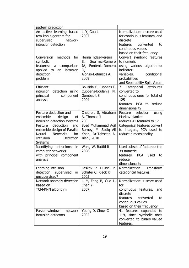
Table 2.1 Summary of Reviewed Papers and Data Pre-processing Method

on KDD Cup 99

Title Author Data Pre-processing method

A novel anomaly detection scheme based on principal component classifier

Shyu M, Chen S, Sarinnapakorn K, Chang L 2003

PCA to reduce dimensionality

Adaptive intrusion detection based on machine learning: feature extraction, classifier construction and sequential

Xu X 2006

Principal component analysis (PCA) for feature selection

19

pattern prediction

An active learning based tcm-knn algorithm for supervised network intrusion detection

Li Y, Guo L 2007

Normalization: z-score used for continuous features, and discrete features converted to continuous values based on their frequency

Conversion methods for symbolic features: a comparison applied to an intrusion detection problem

Herna´ndez-Pereira E, Sua´rez-Romero JA, Fontenla-Romero O, Alonso-Betanzos A. 2009

Convert symbolic features to numeric using various algorithms: indicator variables, conditional probabilities and Separability Split Value

Efficient intrusion detection using principal component analysis

Bouzida Y, Cuppens F, Cuppens-Boulahia N, Gombault S 2004

7 Categorical attributes converted to continuous ones for total of 125 features. PCA to reduce dimensionality

Feature deduction and ensemble design of intrusion detection systems

Chebrolu S, Abraham A, Thomas J 2005

Feature selection using Markov blanket reduces 41 features to 17

Feature deduction and ensemble design of Parallel Neural Networks for Intrusion Detection Systems

Syed Muhammad Aqil Burney, M. Sadiq Ali Khan, Dr.Tahseen A. Jilani, 2010

Categorical features convert to integers, PCA used to reduce dimensionality

Identifying intrusions in computer networks with principal component analysis

Wang W, Battiti R 2006

Used subset of features: the 34 numeric features. PCA used to reduce dimensionality

Learning intrusion detection: supervised or unsupervised?

Laskov P, Dussel P, Schafer C, Rieck K 2005

Normalization. Transform categorical features.

Network anomaly detection based on TCM-KNN algorithm

Li Y, Fang B, Guo L, Chen Y 2007

Normalization: z-score used for continuous features, and discrete features converted to continuous values based on their frequency

Parzen-window network intrusion detectors

Yeung D, Chow C 2002

41 features expanded to 119, since symbolic ones converted to binary-valued features.

20

2.4 Time Series Analysis (TSA)

Time Series Analysis consists of methods for analysing the time series data so that

meaningful statistic and data characteristic can be extracted from. Before being able

to infer from the data, a hypothetical probability model must be set up to represent

the data (Brockwell & Davis, 2002). Elsayed et al. (2011) in their research highlighted

that data dimensions of TSA does not necessary include time. It can be applied to

any type of data that can be represented in a sequence or curve.

Time series data often arise when monitoring industrial processes or tracking

corporate business metrics. Time Series Analysis is also used to forecast future

patterns based on past events. The main motivation of Time Series Analysis is to do

forecast, this is widely used in the field of statistics, econometrics, quantitative

finance and seismology.

In the context of signal processing, communication and control engineering

it is used for signal detection and estimation, while in the context of data mining,

pattern recognition and machine learning, TSA can be used for classification, which

is known as Time Series Classification (TSC).

2.4.1 Time Series Classification (TSC)

In a paper by (Amr, 2012), a new form of a classification technique that new

algorithms or adapting existing machine learning methods to suit time-series data is

introduced and it is known as the Time-Series Classification (TSC) techniques.

Chaovalitwongse et al. (2007) in their research uses the K-Nearest Neighbour (K-NN)

and the Dynamic Time Warping distance (DTW) as the TSC techniques to classify the

abnormal brain activities.

Amr (2012) categorised the TSC in three manners depending on the metric

used for classification. Distance based classification is the classification algorithms

that are based on the distances between the data. One of the most famous distance

based classification algorithms is the k-nearest algorithm. Before passing to the

21

classification algorithm, Feature-based time-series classification requires data to be

transformed from time-series data to feature-set. In addition to above two

classification techniques, model based classification technique requires the modelling

of a data within a class and the new data is classified according to best-fit model.

2.4.2 Distance Similarity Measure

The definition of a distance measure includes three requirements. To define these

requirements, the function dist () is defined to takes as input two sequence 𝑋 =

{𝑥1, 𝑥2, … , 𝑥𝑁} and 𝑌 = {𝑦1, 𝑦2, … , 𝑦𝑀}, and returns the value of the distance. Then,

the requirements for a distance measure are as follows:

1) Non-negativity: The distance between X and Y must be a non-negative value

where it is always greater or equal to zero.

𝑑𝑖𝑠𝑡(𝑋, 𝑌) ≥ 0

2) Identity of indiscernible: The distance between X and Y is equal to zero if and

only if A is equal to B.

𝑑𝑖𝑠𝑡(𝑋, 𝑌) = 0 𝑖𝑓𝑓 𝑋 = 𝑌

3) Symmetry: The distance between X and Y is equal to the distance between Y

and X.

𝑑𝑖𝑠𝑡(𝑋, 𝑌) = 𝑑𝑖𝑠𝑡(𝑌, 𝑋)

Distances which conform to at least these three requirements are known as distance

measures(Weller-Fahy et al., 2014).

a) Euclidean Distance

This distance is commonly accepted as the simplest distance between

sequences. The distance between A and B is defined by

𝑑𝑖𝑠𝑡(𝑋, 𝑌) = √∑(𝑥1. 𝑦1)2 + ⋯ + ∑(𝑥𝑖 . 𝑦𝑖)2

b) Cosine Similarity

Cosine Similarity is the measure of calculating the difference of angle between

two vectors. Similarity between X and Y is defined by

𝑠𝑖𝑚(𝑋, 𝑌) = cos(𝜃) = 𝑋 . 𝑌

|𝑋||𝑌|

22

c) Dynamic Time Warping (DTW)

Dynamic Time Warping (DTW) is an algorithm used to find an optimal alignment

between two given time series data under certain restrictions. The time series,

which may be or not in the same length or phase are aligned and warped. When

DTW is first introduced in the 60s, it was applied in comparing or recognizing

speech patterns. In the domain of financial market forecasting, DTW is applied

to improve the fluctuation prediction of the YEN-Dollar market (Kia et al., 2013).

Gillian et al., (2011) implement DTW-based classification in the context of

biology and medicine where DTW is used to distinguish the 8 different items of

the Wolf Motor Function Test being performed, by collecting the time series

generated by an accelerometer placed on the arm.

The Dynamic Time Warping (DTW) method depends on the similarity of

shape between time series. Unlike Euclidean distance, the temporal relationship

between corresponding points in the two time series is maintained by time axis

that are nonlinearly ‘‘warped’. In order to find the similarity between time series,

the DTW algorithm ensures minimum distance between the aligned points (the

so-called warping path) by finding the alignment, and by performing this,

it ’’warps’’ the axis, choosing the best alignment path, and then generates a

distance measure between the two sequences (Muscillo et al., 2011).

Figure 2.1 shows two sequences A and B that were arranged on the sides

of grid, with sequence A on top and sequence B the left. The minimum value

for the sum of the distance between the individual elements is then divided by

the sum of the weighting function. The weighting function is the function used

to normalise the path length between sequence A and sequence B.

23

Figure 2.2 Matrix Representation of Two Sequence A and B

Source: 1 http://www.psb.ugent.be/cbd/papers/gentxwarper/DTWalgorithm.htm

Let X and Y be two discrete time series polled with the same sampling rate,

and with different lengths, being 𝑋 = {𝑥1, 𝑥2, … , 𝑥𝑁} the input signal and 𝑌 =

{𝑦1, 𝑦2, … , 𝑦𝑀} the reference signal. A matrix 𝑑(𝑖, 𝑗) ∈ 𝑅(𝑁 × 𝑀) is constructed in the

first step of the algorithm, in which the distance between the 𝑖th element of the

sequence 𝑋 and the 𝑗th element of 𝑌 is represented by each element in the matrix.

The Dynamic Programming algorithm looks for a DTW distance function between the

two time series, by minimizing a cost function specifically calculated on the matrix 𝑑.

This cost function is created through the generation of an alignment path (warping

path, W) between the time series. This alignment path defines the correspondence

of an element 𝑥𝑖 to 𝑦𝑗 with the condition that both the first and the last elements of

X and Y are aligned. Intuitively, 𝑑 is composed of small values when sequences are

similar, or large values if they are different. Figure 2.3 illustrates the algorithm

involved to perform DTW to compute the similarity measure between two sequences.

24

Figure 2.3 Algorithm to Perform DTW

Source: A global averaging method for dynamic time warping, with applications to

clustering

2.4.3 Review of TSC for classification

He et al. (2008) in aiming at traffic features of a large-scale communication network,

make every traffic feature a simple time series. The authors then take multiple traffic

feature as a whole to analyse and study through multiple time series data mining. In

this research paper, the approach of applying multiple time series data mining to

large-scale network traffic analysis is done in 5 steps:

i. Compute entropy of several flow level traffic features collected over each time

bin

ii. Apply Principal Component Analysis and subspace method to entropy time

series

iii. Apply time frequency analysis method and Piecewise Aggregate

Approximation and Symbolic Aggregate approximation to anomaly time series.

iv. Apply association rule mining to symbolic sequence.

v. Real-time monitoring with valid motif pattern.

25

Gillian, Knapp, and Modhrain (2011) presented a novel algorithm based on

Dynamic Time Warping (DTW) and extended it to classify any N-dimensional signal.

Musical gestures exhibits by a musician is still considered as difficult for a computer

to recognise. This is because the musical gestures are more often than not a cohesive

sequence of movements and not simple single static gestures. To improve the

performance of DTW, the authors adopted the warping path constraint methods. The

time needed for the computation of DTW is greatly reduced as there is no additional

need to construct a big proportion of the matrix when the warping window is small.

Gillian et al. (2011) n their research also highlighted the advantage of using the DTW

algorithm in related to the template (i.e. musical gesture in this research) where it

can be computed independently. This strait greatly utilizes new machines having

features of multi-threading, i.e. training can be done in parallel. The authors also

compare the implementation of DTW classification to other machine learning

algorithms such as ANN, where adding or removing an existing gesture are

inconvenient as entire system would need to be retrained.

Chaovalitwongse et al. (2007) in their research aim to develop a classification

technique that used to classify normal and abnormal or epileptic brain activities. The

authors use the approach of K-nearest Neighbour (k-NN) algorithm, Dynamic Time

Warping (DTW) and chaos theory in developing the novel classification techniques.

The first step, measure of chaos, known as the short-term maximum Lyapunov

exponent is estimated to quantify the chaoticity of the attractor. Then the EEG data

undergoes classification using the KNN classification and three similarity measure -

DTW, T-Statistical (Index) Distance and Euclidean Distance (ED) are used. The

authors state that the KNN classification with DTW as the similarity measure achieves

its best performance of 84% in sensitivity and a specificity of 75% when k=3.

In this research paper, distance-based time-series classification with k-NN

algorithm as classification technique and DTW as the similarity measure of two

sequences is selected. Conventionally, the Euclidean Distance (ED) serves as the

similarity measure, however the DTW, which provides a better elastic similarity

measure is trusted overcome the shortcoming of the conventional ED (Amr, 2012).

26

2.5 Classification Techniques

An algorithm that implements classification, especially in a concrete implementation,

is known as a classifier. The term "classifier" sometimes also refers to the

mathematical function, implemented by a classification algorithm that maps input

data to a category.

2.5.1 Classification of Data

Data classification involved a two-step process. In the first step, by describing

a predetermined set of data classes, a classifier is built. Classification algorithms then

build the classifier by analysing a learning (training) set and their features (Stolfo et

al., 1999). The features may be continuous, categorical or binary.

Supervised learning is the machine learning task of inferring a function from

labelled training data. The training data consists of a set of training examples. A

labelled data set with a huge number of instances with n features are illustrated in

table 2.2.

Table 2.2 Instances with Known Label

Data in standard format

Instance Feature 1 Feature 2 … Feature n Class

1 Xxx x Xx Normal

2 Xxx X Xx Abnormal

3 Xxx X Xx Normal

… Xxx X Xx Abnormal

y

Precise network traffic classification is vital as it aid to umpteen network activities

(Karagiannis, Papagiannaki, and Faloutsos, 2005). Stated below are few common

goals of accurate network classification:

a) Identification of application and user usage and trends:

27

The network administrator is able to look and inspect on the usage and trends.

This helps to ensure steady and quality of service provided as he can aggregate

suitable bandwidth according to demand for users or applications with higher

usage.

b) Identification of emerging applications

Accurate identification of new network applications can highlight frequent

emergence of disruptive applications that often rapidly alter the dynamics of

network traffic, and sometimes bring down valuable Internet services.

c) Accounting

Knowing the applications their subscribers are using may be of vital interest for

application-based accounting and charging or even for offering new products.

d) Anomaly Detection

Anomaly in a network traffic often indicate the propagation of unusual and

abnormal behaviour. Diagnosing anomalies are crucial for both network

administrator and user to ensure data confidentiality, integrity and availability.

2.5.2 k-Nearest Neighbour (k-NN)

Wu et al.(2008) provide a thorough explanation on how the k-NN algorithm is carried

out in their paper. The three key elements involved in k-NN are:

i. A set of labelled data, e.g., a set of stored records

ii. A distance or similarity metric to calculate the distance between the data

iii. The number of nearest neighbour, k

Given a labelled sequence data set D, a positive integer k, and a new

sequence z to be classified, the k-NN classifier finds the k nearest neighbours of z in

D, k-NN (z), the k-NN algorithm calculate the similarity (distance) between z and D

and returns the dominating class label in the neighbourhood as the label of z. KNN

is a lazy learning method and does not pre-compute a classification model

28

(Zhengzheng Xing, 2010). Figure 2.4 illustrates the process involved during the

execution of a k-NN algorithm.

Figure 2.4 The k-nearest neighbor classification algorithm

2.4.2 Review of k-Nearest Neighbour (k-NN) with Dynamic Time Warping

(DTW) as similarity measure

Although not much attention was given to DTW as the similarity measure for KNN in

the past, there is still quite a number that research on the possibility of the pair. Kia,

SamanHaratizadeh, and HadiZare (2013) uses k-NN and DTW to improve the

fluctuation prediction and to have better evaluation parameters in the literature of

financial market forecasting comparing to other researchers. A 500 sequences of 30

element exchange rate are built based on a data set 15331 USD/JPY exchange rate

records. The authors found a promising result of an improvement in directional

prediction compared to other researchers’ method which is one the most cited

research in the field of financial prediction using newer artificial intelligence and data

mining technique methodologies.

2.5.3 Review of Network Traffic Classification

Panda et al., 2010 apply discriminative multinomial Naïve Bayes with various filtering

analysis to build a network intrusion detection system. By using Principal Component

Analysis (PCA) as a filtering approach, the authors combines both of PCA and

discriminative parameter learning using Naïve Bayes (DMNB) classifier.

29

Before the data are classified, they undergo supervised and unsupervised

data filtering like the PCA, Random Projection (RP) and Nominal to Binary (N2B). The

discriminative parameter learning method learns parameters by discriminatively

computing frequencies from intrusion data. Table 2.3 below shows the result of the

proposed algorithm.

Table 2.3 Results for Various Algorithms

Classifier Detection Accuracy (%) False Alarm Rate in %

Discriminative Multinomial Naïve Bayes + PCA

94.84 4.4

Discriminative Multinomial Naïve Bayes + RP

81.47 12.85

Discriminative Multinomial Naïve Bayes + N2B

96.5 3.0

In the research paper by (Ibrahim et al., 2013), Self-Organization Map (SOM)

Artificial Neural Network (ANN) is performed on the intrusion database (KDD99 and

NSL-KDD). The goal of SOM is to transform an input data set of arbitrary dimension

to a one- or two-dimensional topological map. By building a topology preserving map,

it aims to observe the underlying structure of the input data set. The authors believed

that even in the absence of complete data or distorted data, the Neural Network

would be capable of analysing data from the network. Table 2.4 below shows the

result obtained by the author using SOM-ANN algorithms on the NSL-KDD dataset.

Table 2.4 Result for Application of SOM-ANN Algorithms

Classifier Successful Detection Rate (%)

SOM 68.88

2.6 Summary

In this chapter, the IDS is covered to provide readers a basic knowledge on the use

of anomaly detection. IDS has grown from time to time to suit the change of

30

technology. However, the flaws of IDS are yet to be overcome. Data classification is

also briefly discussed to show its role in an IDS.

After reviewing related works from the field, Time Series Classification (TSC)

is believed to have its potential for network traffic analysis. A mixed model of k-NN

algorithm and DTW is chosen in this research paper to classify network traffic

activities. Because the temporal dimension warping, DTW is good for classifying

sequences that have different frequencies or those that are out of phase.

CHAPTER 3

METHODOLOGY

3.1 Chapter Overview

This chapter covers the methodology used to perform this research. It is arranged in

the order of 3.2 Procedures, 3.3 Experimental Setting, 3.4 Validations of Findings and

finally the Summary. In 3.2, discussion is on the procedures involved in carrying out

this research. Followed by 3.3, where the experimental setting to validate the

proposed techniques will be discussed. After the experiment is carried out, it is vital

to validate the findings, methods of validation will be discussed in 3.4.

3.2 The Research Program of Work

Figure 3.3 Overall Framework used in this Research

Figure 3.1 illustrates the overall framework used within this research paper. Apart

from first experiment where all categorical features are removed from the train and

test set, all the train and test set undergoes data preprocessing step where

categorical data are converted into a numerical value based on three different

32

approaches, simple, probability and entropy conversion. These data are then

normalized using min-max normalization method. The converted and normalized

dataset was also undergone feature selection technique by Information Gain (IG)

and Correlation Feature Selection (CFS) generating train set and test set.

To achieve the objective stated in section 1.4, the methodology will be carried

out in two phases. Phase 1 (Figure 3.2) involved the identification of the best

approach to solve the problem “How to represent network traffic data into point

series form”.

Figure 3.2 Phase I of the research

Three sub phases are then further divided from it:

Sub-phase I involved the representation of the features extracted (as

provided in the dataset) in the form of point series by investigating and implementing

various feature transformation techniques. Throughout this research paper, only

secondary data set will be used. No data generation is involved. The data set selected

is the improved version of the famous KDD’99 data set - The NSL-KDD Data Set. The

mentioned original NSL-KDD data set can be obtained from the link:

<http://nsl.cs.unb.ca/NSL-KDD/>. In this phase, the original dataset with categorical

numeric and nominal attribute is transformed to be represented in a point series

form. For the first attempt, categorical data will be left out. Experimentations to

evaluate the performances of the selected feature transformation techniques

identified will be performed using a TSC technique which is Dynamic Time Warping

(DTW) as a similarity measure for the classification of network traffic activities using

the K-NN algorithm. Distance similarity measure, Euclidean Distance and Cosine

Similarity will also be incorporated into the K-NN classification (Figure 3.3).

33

Figure 3.3 Sub-phase I of the research

Sub-phase II involve the simple conversion of categorical data. In this phase

categorical data will be converted using alphabetically simple conversion method.

The distinct value within each feature will be arranged alphabetically and a

corresponding sequence of integer will be assigned to each of them. Then

classification using KNN with three different similarity measures will be applied to the

data. The framework of sub-phase II is illustrated in Figure 3.4.

34

Figure 3.4 Sub-phase II of the research

Sub-phase III involve the entropy conversion and the probability conversion

for categorical data (Figure 3.5).

35

Figure 3.5 Sub-phase III of the research

Phase II works with selecting features from the converted and normalized

dataset from phase I by using two feature selection methods which is Information

Gain (IG) and Correlation Feature Selection (CFS) (Figure 3.6).

36

Figure 3.6 Phase II of the research

37

3.3 Experimental Setting

To achieve the objectives stated in Section 1.4, two sets of experiments will be carried

out. Experiment I is to determine the best feature transformation technique.

In this research paper, a 10-fold cross validation approach will be used to

assess the result and how accurate the performance of predicted model is. A test set

containing known labelled (classified) data is used. The classifier will then be trained

to the test set using the train set. The NSL-KDD data set is subdivided into ten sub

dataset which in this research paper, one dataset will be used as test set and the

remaining nine sets function as training set. The iterations are repeated by ten times

with each iteration replaced with another dataset without repeating.

A mixed model of k-NN and DTW algorithm will be used to measure the

similarity of the data sequence and classify them. As proposed, the DTW algorithm

will be used as a similarity measure for two sequences, and k-NN is used to train and

classify the data to determine the class label.

Experiment II is designed to compare the performances of the proposed TSC

based approach compared to other approaches found in the literature.

3.4 Experiment Requirement

To implement the proposed research methodology of KNN-DTW, there are a few

hardware and software requirements that needed to be met.

3.4.1 Hardware Requirement

Listed below are the hardware used within a laptop to carry out the experiment:

Intel Core i7-4510U @2.3GHz

3.4.2 Software Requirement

Matlab 2014a is used in the research paper to carry out all the experiments.

38

3.5 Performance Measure for Classification

To measure the quality of performance of the proposed approach, the result of the

proposed model will be compared to ground truth (labelled data). For the NSL-KDD

data set, all the data were labelled, which is, the class of each instance is known.

Each instance is labelled as normal or anomaly. In table 3.1, the possible outcomes

of the nature of result of the proposed model are shown.

Table 3.1 Possible Outcomes

Predicted

Positive Negative

Truth Positive True Positive, tp False Negative, fn

Negative False Positive, fp True Negative, tn

Detection rate (DR) is calculated as the ratio between the number of correctly

detected intrusions and the total number of intrusions. Note: Detection Rate is also

known as the measure of sensitivity in some of the papers in Literature Review.

𝐷𝑒𝑡𝑒𝑐𝑡𝑖𝑜𝑛 𝑅𝑎𝑡𝑒, 𝐷𝑅 = 𝑡𝑝

𝑓𝑛 + 𝑡𝑝

False positive rate (FP) is calculated as the ratio between the numbers of

normal traffic that are incorrectly classified as intrusions and the total number of

normal traffic. Note: False Positive is also known as the measure of specificity in

some of the papers in Literature Review.

𝐹𝑎𝑙𝑠𝑒 𝑃𝑜𝑠𝑖𝑡𝑖𝑣𝑒, 𝐹𝑃 = 𝑓𝑝

𝑡𝑛 + 𝑓𝑝

Accuracy indicates how correct the detection technique is. Performance,

precision is measured in percentage of accuracy, which is also the ratio between

correct detections and total detections obtained.

𝐴𝑐𝑐𝑢𝑟𝑎𝑐𝑦, 𝑎 = 𝑡𝑝 + 𝑡𝑛

𝑓𝑝 + 𝑓𝑛 + 𝑡𝑝 + 𝑡𝑛

39

The value achieves for Accuracy should not exceed 100%. The lack in

accuracy causes false positive.

3.6 Summary

To summarize, the procedures mentioned above are carried out to ensure that the

objective of the research can be achieved. The processes involved in each phase are

laid out in detail, and illustration is provided to aid understanding.

CHAPTER 4

IMPLEMENTATION OF THE PROPOSED APPROACH

4.1 Chapter Overview

In this chapter, experimental setup for the research to be carried out is presented.

Section 4.2 will explain in detail how the data set is pre-processed, whereas Section

4.3 discuss how the experiment is set up. And lastly, the summary made from current

studies and experiments is presented in Section 4.4.

4.2 Data Pre-processing

Phase I involved the representation of features of the dataset in the form of point

series data. The data set selected which is the NSL-KDD data set contains a total of

148517 entries and each with 41 features and one class label which label the data

as normal or anomaly. In this phase involved two tasks which are data conversion

and data normalization.

4.2.1 Conversion of data

Before proceeding to the experimental setting, the NSL-KDD dataset is first pre-

processed. The first step of data-pre-processing in this research paper involved the

conversion of feature type. First, identification of the feature type must take place.

Table 4.1 Features Name and Type

Features Type Features Type

duration Numeric count Numeric

protocol_type Nominal srv_count Numeric

service Nominal serror_rate Numeric

flag Nominal srv_serror_rate Numeric

src_bytes Numeric rerror_rate Numeric

dst_bytes Numeric srv_rerror_rate Numeric

land Nominal same_srv_rate Numeric

wrong_fragment Numeric diff_srv_rate Numeric

urgent Numeric srv_diff_host_rate Numeric

hot Numeric dst_host_count Numeric

num_failed_logins Numeric dst_host_srv_count Numeric

logged_in Numeric dst_host_same_srv_rate Numeric

num_compromised Numeric dst_host_diff_srv_rate Numeric

root_shell Numeric dst_host_same_src_port_rate

Numeric

su_attempted Numeric dst_host_srv_diff_host_rate

Numeric

num_root Numeric dst_host_serror_rate Numeric

num_file_creations Numeric dst_host_srv_serror_rate Numeric

num_shells Numeric dst_host_rerror_rate Numeric

num_access_files Numeric dst_host_srv_rerror_rate Numeric

num_outbound_cmds Numeric class Nominal

is_host_login Nominal

is_guest_login Nominal

Table 4.1 shows the features of the NSL-KDD data and the feature’s type

which is categorized as numeric or nominal. For features that are nominal and

contains no numeric representation, conversion to numeric value is made so that

representation of the features in point series data is made possible. Out of these 41

features and one class label, seven of the features are having nominal data. Followed

by three having not numeric data value. This three features, namely “protocol_type”,

“service” and “flag”. In this section, three conversion methods were applied to the

three categorical features mentioned above, which is the simple conversion,

probability conversion and lastly entropy conversion.

42

a) Alphabetical simple conversion

First method, simple conversion involves the process of assigning the categorical

data value alphabetically with numbers. First categorical data, “protocol_type”

contains three distinct values, which are “tcp”, “icmp” and “udp”. These values

are first arranged in alphabetically order.

Table 4.2 Alphabetically Simple Conversion of "protocol_type"

Existing Data After

Conversion

icmp 0

tcp 1

udp 2

Table 4.2 shows the available existing data for the feature “protocol_type”

and its numerical representation after conversion is done. The data “icmp” is

converted to “0”, whereas “tcp” is converted to “1” and “udp” is converted to “2”.

The next categorical data is the “service” feature which contains a total

of 70 distinct categorical values. After arranging the data in alphabetical order,

the data “aol” is converted to “0”, whereas “auth” is converted to “1” and “bgp”

is converted to “2” and so on. Table 4.3 below shows the existing data for the

feature “service” and its numerical value after conversion.

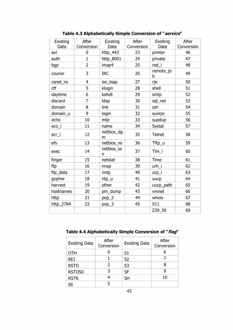
43

Table 4.3 Alphabetically Simple Conversion of "service"

Existing Data

After Conversion

Existing Data

After Conversion

Existing Data

After Conversion

aol 0 http_443 23 printer 46

auth 1 http_8001 24 private 47

bgp 2 imap4 25 red_i 48

courier 3 IRC 26 remote_job

49

csnet_ns 4 iso_tsap 27 rje 50

ctf 5 klogin 28 shell 51

daytime 6 kshell 29 smtp 52

discard 7 ldap 30 sql_net 53

domain 8 link 31 ssh 54

domain_u 9 login 32 sunrpc 55

echo 10 mtp 33 supdup 56

eco_i 11 name 34 Systat 57

ecr_i 12 netbios_dgm

35 Telnet 58

efs 13 netbios_ns 36 Tftp_u 59

exec 14 netbios_ssn

37 Tim_i 60

finger 15 netstat 38 Time 61

ftp 16 nnsp 39 urh_i 62

ftp_data 17 nntp 40 urp_i 63

gopher 18 ntp_u 41 uucp 64

harvest 19 other 42 uucp_path 65

hostnames 20 pm_dump 43 vmnet 66

http 21 pop_2 44 whois 67

http_2784 22 pop_3 45 X11 68

Z39_50 69

Table 4.4 Alphabetically Simple Conversion of "flag"

Existing Data After

Conversion Existing Data

After Conversion

OTH 0 S1 6

REJ 1 S2 7

RSTO 2 S3 8

RSTOS0 3 SF 9

RSTR 4 SH 10

S0 5

44

In Table 4.4, the feature “flag” contains 11 distinct data values, conversion

of the existing data to numeric representation is being made. The data “OTH” is

converted to “0”, whereas “REJ” is converted to “1” and “RSTO” is converted to

“2” and so on.

After the conversion of the categorical data using simple conversion, the

data can then be represented in a point series format. Figure 4.1 below illustrates

10 point series data generated results from the conversion method discussed.

There are a total of 41 features present for one point series.

Figure 4.1 Point Series Data with Simple Conversion

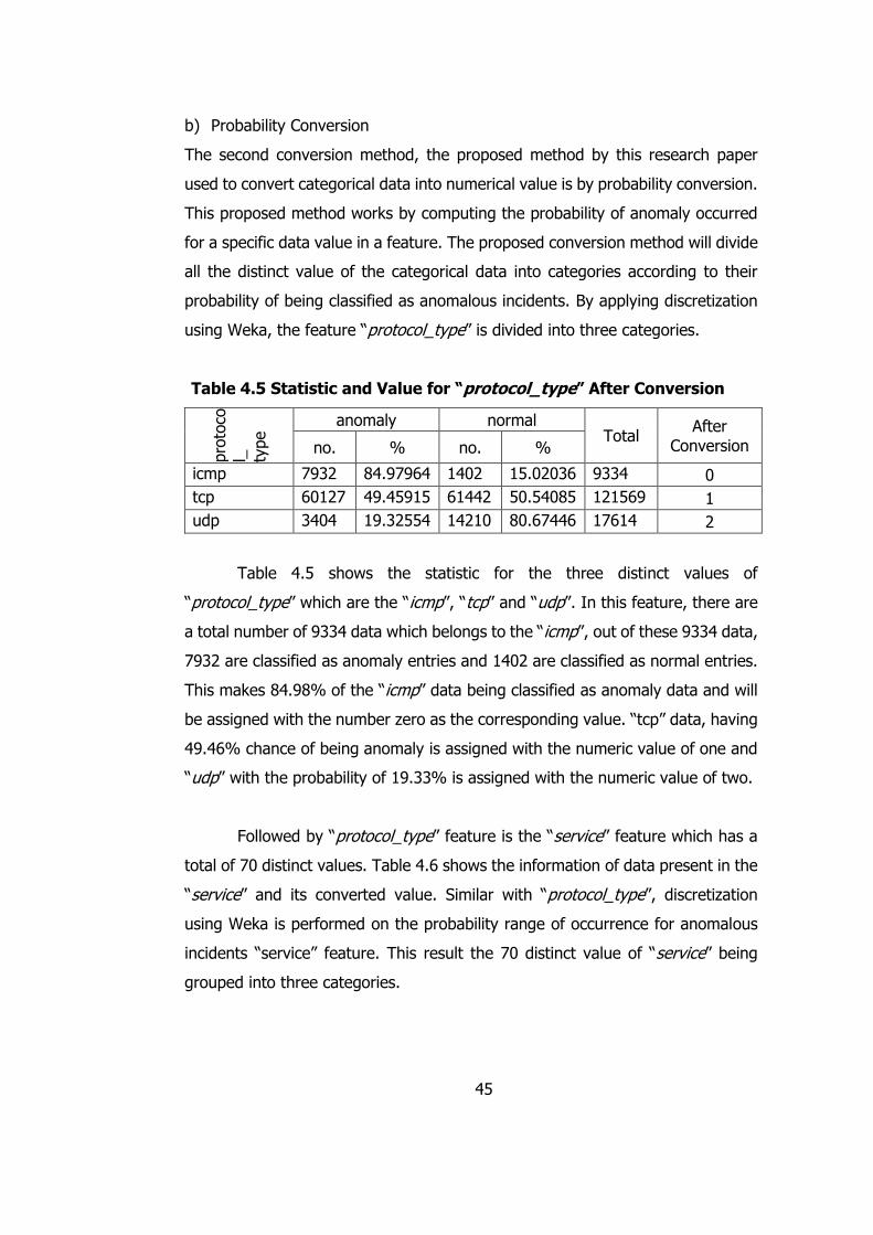
45

b) Probability Conversion

The second conversion method, the proposed method by this research paper

used to convert categorical data into numerical value is by probability conversion.

This proposed method works by computing the probability of anomaly occurred

for a specific data value in a feature. The proposed conversion method will divide

all the distinct value of the categorical data into categories according to their

probability of being classified as anomalous incidents. By applying discretization

using Weka, the feature “protocol_type” is divided into three categories.

Table 4.5 Statistic and Value for “protocol_type” After Conversion

pro

toco

l_

type anomaly normal

Total After

Conversion no. % no. %

icmp 7932 84.97964 1402 15.02036 9334 0

tcp 60127 49.45915 61442 50.54085 121569 1

udp 3404 19.32554 14210 80.67446 17614 2

Table 4.5 shows the statistic for the three distinct values of

“protocol_type” which are the “icmp”, “tcp” and “udp”. In this feature, there are

a total number of 9334 data which belongs to the “icmp”, out of these 9334 data,

7932 are classified as anomaly entries and 1402 are classified as normal entries.

This makes 84.98% of the “icmp” data being classified as anomaly data and will

be assigned with the number zero as the corresponding value. “tcp” data, having

49.46% chance of being anomaly is assigned with the numeric value of one and

“udp” with the probability of 19.33% is assigned with the numeric value of two.

Followed by “protocol_type” feature is the “service” feature which has a

total of 70 distinct values. Table 4.6 shows the information of data present in the

“service” and its converted value. Similar with “protocol_type”, discretization

using Weka is performed on the probability range of occurrence for anomalous

incidents “service” feature. This result the 70 distinct value of “service” being

grouped into three categories.

46

Table 4.6 Statistic and Value for “service” After Conversion

Service

anomaly normal No.

Aft

er

Convers

ion

Total no. % no. %

aol 2 100 0 0 2

0 63758

bgp 756 100 0 0 756

courier 774 100 0 0 774

csnet_ns 579 100 0 0 579

ctf 604 100 0 0 604

daytime 549 100 0 0 549

discard 564 100 0 0 564

echo 471 100 0 0 471

efs 518 100 0 0 518

exec 501 100 0 0 501

gopher 552 100 0 0 552

harvest 2 100 0 0 2

hostnames 483 100 0 0 483

http_2784 1 100 0 0 1

http_443 566 100 0 0 566

http_8001 2 100 0 0 2

iso_tsap 735 100 0 0 735

klogin 454 100 0 0 454

kshell 323 100 0 0 323

ldap 429 100 0 0 429

login 458 100 0 0 458

mtp 471 100 0 0 471

name 488 100 0 0 488

netbios_dgm 430 100 0 0 430

netbios_ns 383 100 0 0 383

netbios_ssn 377 100 0 0 377

netstat 386 100 0 0 386

nnsp 672 100 0 0 672

nntp 317 100 0 0 317

pm_dump 21 100 0 0 21

pop_2 91 100 0 0 91

printer 80 100 0 0 80

rje 94 100 0 0 94

sql_net 263 100 0 0 263

47

supdup 571 100 0 0 571

systat 509 100 0 0 509

uucp 830 100 0 0 830

uucp_path 735 100 0 0 735

vmnet 660 100 0 0 660

whois 733 100 0 0 733

Z39_50 907 100 0 0 907

sunrpc 539 99.81481 1 0.185185 540

link 515 99.8062 1 0.193798 516

imap4 950 99.6852 3 0.314795 953

remote_job 91 98.91304 1 1.086957 92

ssh 332 98.51632 5 1.48368 337

shell 77 95.06173 4 4.938272 81

domain 582 93.87097 38 6.129032 620

ecr_i 3591 93.78428 238 6.215722 3829

private 24793 93.11225 1834 6.887746 26627

eco_i 4325 89.21205 523 10.78795 4848

time 609 88.26087 81 11.73913 690

pop_3 1089 84.87919 194 15.12081 1283

telnet 3018 75.8482 961 24.1518 3979

auth 767 75.04892 255 24.95108 1022

finger 1311 68.89122 592 31.10878 1903

1 17271

ftp 1480 60.50695 966 39.49305 2446

tim_i 8 57.14286 6 42.85714 14

other 2528 48.64345 2669 51.35655 5197

ftp_data 2407 31.21515 5304 68.78485 7711

X11 17 19.31818 71 80.68182 88

2 67488

smtp 600 7.275373 7647 92.72463 8247

http 3469 7.19844 44722 92.80156 48191

IRC 4 2 196 98 200

urp_i 8 1.28 617 98.72 625

domain_u 11 0.110697 9926 99.8893 9937

ntp_u 0 0 178 100 178

red_i 0 0 8 100 8

tftp_u 0 0 4 100 4

urh_i 0 0 10 100 10

Table 4.6 presents the statistic of the data exist in the “service” feature.

A total of 55 data have probability more that 75% belongs to the anomaly class.

48

Thus, 63758 data are converted to the numeric value of zero. Whereas there are

5 data that has probability ranging from 31.22% to 68.89% being classified as

anomaly entries are converted to a numeric value of one. The rest of the data,

having the probability value of 0.00% to 19.32% is converted to the numeric

value of two.

Table 4.7 Statistic and Value for “flag” After Conversion

Flag anomaly normal

No. After Conversion

Total no. % no. %

SH 342 99.4186 2 0.581395 344

0 58169

RSTOS0 104 99.04762 1 0.952381 105

S0 36510 99.03971 354 0.960286 36864

RSTR 2900 93.85113 190 6.148867 3090

RSTO 2114 90.53533 221 9.464668 2335

S3 249 83.55705 49 16.44295 298

REJ 12355 81.91341 2728 18.08659 15083

OTH 39 78 11 22 50

SF 16820 18.72634 73000 81.27366 89820

1 90348 S2 15 10.56338 127 89.43662 142

S1 14 3.626943 372 96.37306 386

After performing discretization, the probability range for the occurrence

of anomalous incidents is divided into two categories, where data having the

probability of more than 78% belongs to the anomaly class being grouped into

one category. This category is assigned with the numeric value of zero and the

other group assigned with the numeric value of one have the probability ranging

from 3.63% to 18.73% (Table 4.7). Figure 4.2 below shows 10 point series data

generated using probability conversion techniques for categorical data.

49

Figure 4.2 Point Series Data with Probability Conversion

c) Entropy Conversion

The third conversion method used to convert the categorical features is by

entropy conversion which is converting the different value of the categorical data

into a sequence of integer. However, unlike the simple conversion, entropy

conversion first performs calculation of the entropy of value within a feature.

Then the values are sorted according to their entropy where lowest entropy has

the highest ranking of zero and so forth. The entropy value is computed

according to the formula:

𝐸𝑛𝑡𝑟𝑜𝑝𝑦, 𝐸𝑛𝑡 = −[(𝑥

𝑁 × log2

𝑥

𝑁) + (

𝑦

𝑁 × 𝑙𝑜𝑔2

𝑦

𝑁)]

Where x: total number of anomalous incidents of that particular value within a

feature

y: total number of normal incidents of that particular value within a

feature

N: total number of entries of that particular value within the feature

50

Table 4.8 Entropy of “protocol_type” Data and Corresponding Converted

Value

protocol_ type

anomaly normal total Entropy After Conversion

icmp 7932 1402 9334 0.61 0

udp 3404 14210 17614 0.71 1

tcp 60127 61442 121569 1.00 2

Table 4.8 shows that the icmp has the highest ranking with the lowest entropy

value of 0.61, thus is being converted to zero, whereas udp is converted to the

numeric value of one and tcp is being converted to the number two for having

the lowest ranking.

Table 4.9 Entropy of “service” Data and Corresponding Converted Value

Service Anom

aly Normal Total Entropy

After Conversion

aol 2 0 2 0 0

bgp 756 0 756 0 0

courier 774 0 774 0 0

csnet_ns 579 0 579 0 0

ctf 604 0 604 0 0

daytime 549 0 549 0 0

discard 564 0 564 0 0

echo 471 0 471 0 0

efs 518 0 518 0 0

exec 501 0 501 0 0

gopher 552 0 552 0 0

harvest 2 0 2 0 0

hostnames 483 0 483 0 0

http_2784 1 0 1 0 0

http_443 566 0 566 0 0

http_8001 2 0 2 0 0

iso_tsap 735 0 735 0 0

klogin 454 0 454 0 0

kshell 323 0 323 0 0

ldap 429 0 429 0 0

login 458 0 458 0 0

mtp 471 0 471 0 0

name 488 0 488 0 0

netbios_dgm 430 0 430 0 0

51

netbios_ns 383 0 383 0 0

netbios_ssn 377 0 377 0 0

netstat 386 0 386 0 0

nnsp 672 0 672 0 0

nntp 317 0 317 0 0

pm_dump 21 0 21 0 0

pop_2 91 0 91 0 0

printer 80 0 80 0 0

rje 94 0 94 0 0

sql_net 263 0 263 0 0

supdup 571 0 571 0 0

systat 509 0 509 0 0

uucp 830 0 830 0 0

uucp_path 735 0 735 0 0

vmnet 660 0 660 0 0

whois 733 0 733 0 0

Z39_50 907 0 907 0 0

ntp_u 0 178 178 0 0

red_i 0 8 8 0 0

tftp_u 0 4 4 0 0

urh_i 0 10 10 0 0

domain_u 11 9926 9937 0.012466 1

sunrpc 539 1 540 0.019478 2

link 515 1 516 0.020257 3

imap4 950 3 953 0.030698 4

remote_job 91 1 92 0.086504 5

urp_i 8 617 625 0.098831 6

ssh 332 5 337 0.111374 7

IRC 4 196 200 0.141441 8

shell 77 4 81 0.283769 9

domain 582 38 620 0.332546 10

ecr_i 3591 238 3829 0.335949 11

private 24793 1834 26627 0.361721 12

http 3469 44722 48191 0.373286 13

smtp 600 7647 8247 0.376117 14

eco_i 4325 523 4848 0.493487 15

time 609 81 690 0.521815 16

pop_3 1089 194 1283 0.612855 17

X11 17 71 88 0.70808 18

telnet 3018 961 3979 0.797556 19

auth 767 255 1022 0.810502 20

finger 1311 592 1903 0.894425 21

52

ftp_data 2407 5304 7711 0.895641 22

ftp 1480 966 2446 0.967908 23

tim_i 8 6 14 0.985228 24

other 2528 2669 5197 0.999469 25

Table 4.9 shows the distinct data for the feature “service”, a total number of 45

data have entropy value of zero, which are then converted to the numeric value

of zero. The rest is converted according to their ranking where highest entropy

has the lowest ranking. After performing calculation of entropy, the distinct value

within “flag” features are arranged from SH to OTH where SH has the lowest

entropy value and is ranked zero and OTH has the lowest ranking of ten (Table

4.10).

Table 4.10 Entropy of “flag” Data and Corresponding Converted Value

Flag Anomaly Normal Total Entropy After

Conversion

SH 342 2 344 0.051539 0

RSTOS0 104 1 105 0.07762 1

S0 36510 354 36864 0.078149 2

S1 14 372 386 0.224918 3

RSTR 2900 190 3090 0.333326 4

RSTO 2114 221 2335 0.451793 5

S2 15 127 142 0.486604 6

S3 249 49 298 0.644802 7

REJ 12355 2728 15083 0.681968 8

SF 16820 73000 89820 0.695712 9

OTH 39 11 50 0.760168 10

4.2.2 Data Normalization

Having a larger range for a feature tend to give greater weight, thus the data should

be normalized. For distance-based methods, normalization help prevent attributes

with initially, large ranges (e.g., income) from outweighing attributes with initially,

smaller ranges (e.g., binary attributes) (Kumar & Nancy, 2014). There exists many

ways for data normalization, one of which is the min-max normalization method

which preserves the relationships among the original data values.

53

Table 4.11 Features with Minimum and Maximum Value for Simple

Conversion

Features Min

Value Max

Value Features

Min Value

Max Value

duration 0 57715 is_guest_login 0 1

protocol_type 0 2 count 0 511

service 0 69 srv_count 0 511

flag 0 10 serror_rate 0 1

src_bytes 0 1.38E+09 srv_serror_rate 0 1

dst_bytes 0 1.31E+09 rerror_rate 0 1

land 0 1 srv_rerror_rate 0 1

wrong_fragment 0 3 same_srv_rate 0 1

urgent 0 3 diff_srv_rate 0 1

hot 0 101 srv_diff_host_rate 0 1

num_failed_logins 0 5 dst_host_count 0 255

logged_in 0 1 dst_host_srv_count

0 255

num_compromised 0 7479 dst_host_same_srv_rate

0 1

root_shell 0 1 dst_host_diff_srv_rate

0 1

su_attempted 0 2 dst_host_same_src_port_rate

0 1

num_root 0 7468 dst_host_srv_diff_host_rate

0 1

num_file_creations 0 100 dst_host_serror_rate

0 1

num_shells 0 5 dst_host_srv_serror_rate

0 1

num_access_files 0 9 dst_host_rerror_rate

0 1

num_outbound_cmds

0 0 dst_host_srv_rerror_rate

0 1

is_host_login 0 1 class 0 1

Table 4.11 shows the features of the KDD dataset and its corresponding

minimum and maximum value. From the table, at least 13 of the total features has

a wide range of data. After identifying the minimum and maximum value for

respective feature, the data are then scaled to fit in the range of zero and one. Using

the formula,

54

norm_data = 𝑑𝑎𝑡𝑎(𝑓𝑒𝑎𝑡𝑢𝑟𝑒) − 𝑚𝑖𝑛(𝑓𝑒𝑎𝑡𝑢𝑟𝑒)

max(𝑓𝑒𝑎𝑡𝑢𝑟𝑒) − 𝑚𝑖𝑛(𝑓𝑒𝑎𝑡𝑢𝑟𝑒)

Where norm_data is the data after normalization

data(feature) is the data which is supposed to undergo normalization

min(feature) is the minimum value for the respective feature

max(feature) is the maximum value for the respective feature

Subsequently, the data are ready to be represented in curve format.

4.2.3 Feature Selection

Data above were then undergoing three feature selection technique. Information

Gain (IG) and Correlation Feature Selection (CFS) were used in this section. The

original data containing categorical and numeric data are first imported to WEKA for

feature selection.

a) Information Gain (IG)

The original dataset is uploaded to WEKA for feature selection using Information

Gain Method. Attribute evaluator of Information Gain is selected, by default the

search method for it must use Ranker Search method. Figure 4.3 below shows

the snapshot captured during the Information Gain Feature Selection process

using WEKA. After the feature selection process is completed, a table of the

average merit, average ranking for each attribute is listed out in a descending

order.

55

Figure 4.3 Snapshot on WEKA - Information Gain Feature Selection

Table 4.12 Output of Information Gain Feature Selection

average merit average rank attribute

0.781 +- 0 1 +- 0 5 src_bytes

0.625 +- 0.001 2 +- 0 6 dst_bytes

0.62 +- 0.001 3 +- 0 3 service

0.473 +- 0.001 4 +- 0 4 flag

0.46 +- 0.001 5 +- 0 30 diff_srv_rate

0.45 +- 0.001 6 +- 0 29 same_srv_rate

0.427 +- 0.001 7 +- 0 33 dst_host_srv_count

0.391 +- 0.001 8 +- 0 34 dst_host_same_srv_rate

0.372 +- 0.001 9 +- 0 35 dst_host_diff_srv_rate

0.36 +- 0.001 10 +- 0 12 logged_in

0.339 +- 0.001 11 +- 0 23 count

0.337 +- 0.001 12 +- 0 38 dst_host_serror_rate

0.331 +- 0.001 13 +- 0 25 serror_rate

56

0.329 +- 0 14 +- 0 39 dst_host_srv_serror_rate

0.312 +- 0.001 15 +- 0 26 srv_serror_rate

0.248 +- 0.001 16 +- 0 37 dst_host_srv_diff_host_rate

0.185 +- 0.001 17.1 +-0.3 32 dst_host_count

0.184 +- 0.001 17.9 +-0.3 36 dst_host_same_src_port_rate

0.14 +- 0 19 +- 0 31 srv_diff_host_rate

0.091 +- 0.001 20 +- 0 41 dst_host_srv_rerror_rate

0.079 +- 0 21 +- 0 27 rerror_rate

0.077 +- 0 22 +- 0 40 dst_host_rerror_rate

0.072 +- 0 23 +- 0 28 srv_rerror_rate

0.069 +- 0 24 +- 0 24 srv_count

0.058 +- 0 25 +- 0 2 protocol_type

0.034 +- 0.001 26 +- 0 1 duration

0.015 +- 0 27 +- 0 10 hot

0.007 +- 0 28 +- 0 13 num_compromised

0.006 +- 0 29 +- 0 8 wrong_fragment

0.003 +- 0 30 +- 0 16 num_root

0.002 +- 0 31 +- 0 11 num_failed_logins

0.002 +- 0 32 +- 0 19 num_access_files

0.001 +- 0 33 +- 0 17 num_file_creations

0 +- 0 34 +- 0 15 su_attempted

0 +- 0 35 +- 0 14 root_shell

0 +- 0 36.4 +-0.49 7 land

0 +- 0 36.7 +-0.64 21 is_host_login

0 +- 0 37.9 +-0.3 18 num_shells

0 +- 0 39 +- 0 20 num_outbound_cmds

0 +- 0 40 +- 0 22 is_guest_login

0 +- 0 41 +- 0 9 urgent

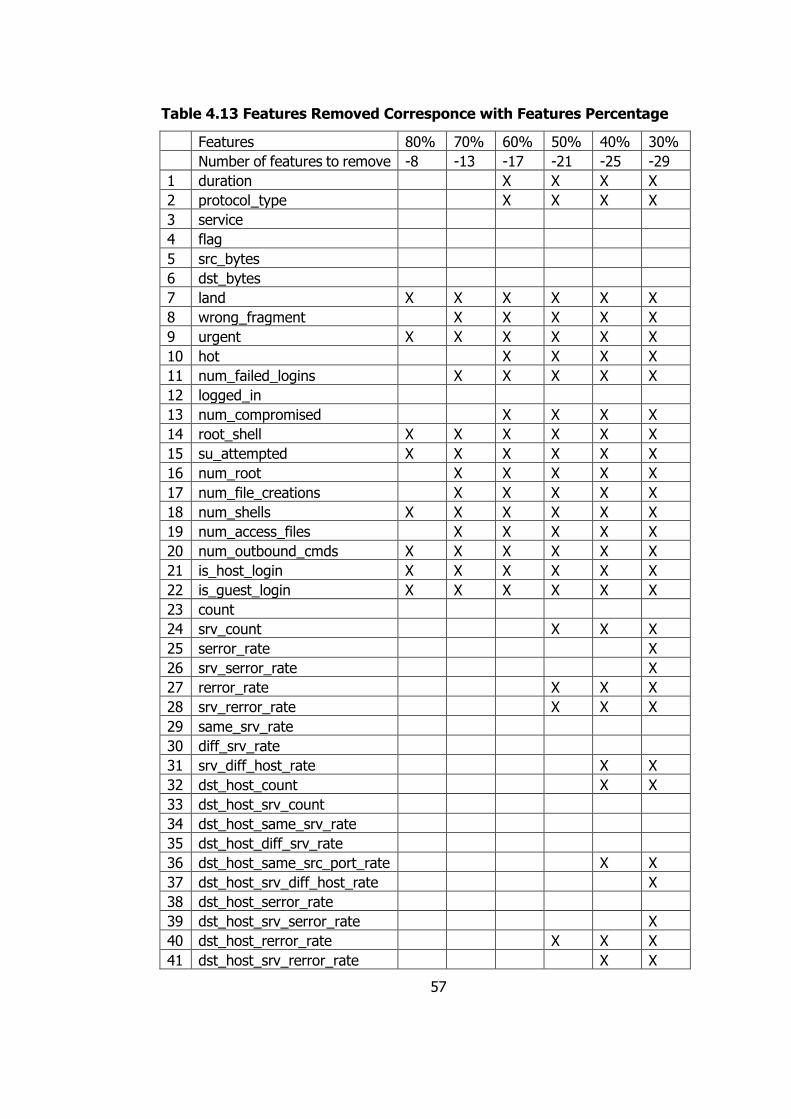
57

Table 4.13 Features Removed Corresponce with Features Percentage

Features 80% 70% 60% 50% 40% 30%

Number of features to remove -8 -13 -17 -21 -25 -29

1 duration X X X X

2 protocol_type X X X X

3 service

4 flag

5 src_bytes

6 dst_bytes

7 land X X X X X X

8 wrong_fragment X X X X X

9 urgent X X X X X X

10 hot X X X X

11 num_failed_logins X X X X X

12 logged_in

13 num_compromised X X X X

14 root_shell X X X X X X

15 su_attempted X X X X X X

16 num_root X X X X X

17 num_file_creations X X X X X

18 num_shells X X X X X X

19 num_access_files X X X X X

20 num_outbound_cmds X X X X X X

21 is_host_login X X X X X X

22 is_guest_login X X X X X X

23 count

24 srv_count X X X

25 serror_rate X

26 srv_serror_rate X

27 rerror_rate X X X

28 srv_rerror_rate X X X

29 same_srv_rate

30 diff_srv_rate

31 srv_diff_host_rate X X

32 dst_host_count X X

33 dst_host_srv_count

34 dst_host_same_srv_rate

35 dst_host_diff_srv_rate

36 dst_host_same_src_port_rate X X

37 dst_host_srv_diff_host_rate X

38 dst_host_serror_rate

39 dst_host_srv_serror_rate X

40 dst_host_rerror_rate X X X

41 dst_host_srv_rerror_rate X X

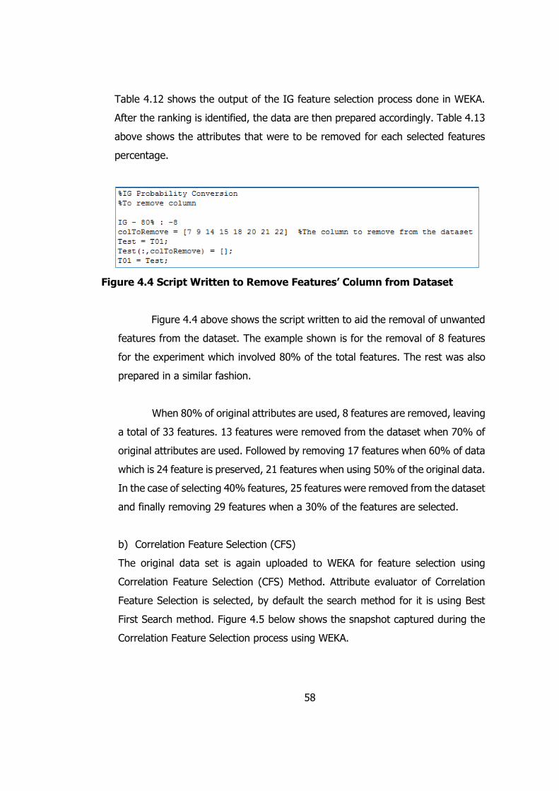
58

Table 4.12 shows the output of the IG feature selection process done in WEKA.

After the ranking is identified, the data are then prepared accordingly. Table 4.13

above shows the attributes that were to be removed for each selected features

percentage.

Figure 4.4 Script Written to Remove Features’ Column from Dataset

Figure 4.4 above shows the script written to aid the removal of unwanted

features from the dataset. The example shown is for the removal of 8 features

for the experiment which involved 80% of the total features. The rest was also

prepared in a similar fashion.

When 80% of original attributes are used, 8 features are removed, leaving

a total of 33 features. 13 features were removed from the dataset when 70% of

original attributes are used. Followed by removing 17 features when 60% of data

which is 24 feature is preserved, 21 features when using 50% of the original data.

In the case of selecting 40% features, 25 features were removed from the dataset

and finally removing 29 features when a 30% of the features are selected.

b) Correlation Feature Selection (CFS)

The original data set is again uploaded to WEKA for feature selection using

Correlation Feature Selection (CFS) Method. Attribute evaluator of Correlation

Feature Selection is selected, by default the search method for it is using Best

First Search method. Figure 4.5 below shows the snapshot captured during the

Correlation Feature Selection process using WEKA.

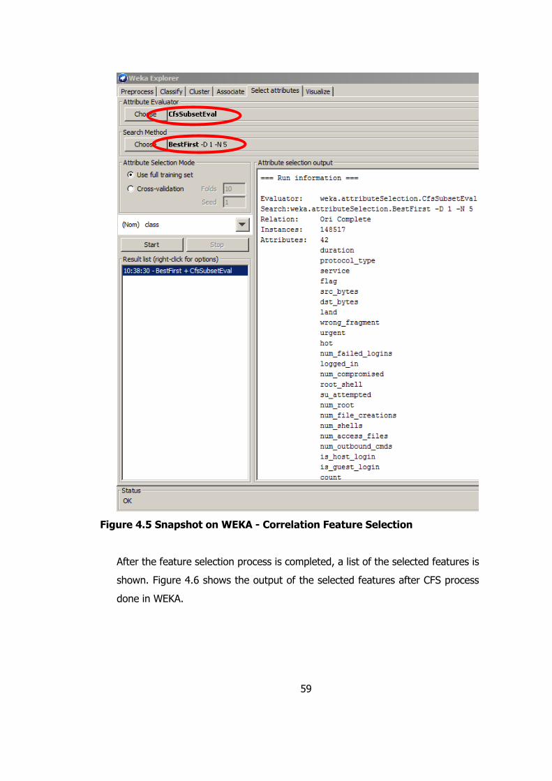
59

Figure 4.5 Snapshot on WEKA - Correlation Feature Selection

After the feature selection process is completed, a list of the selected features is

shown. Figure 4.6 shows the output of the selected features after CFS process

done in WEKA.

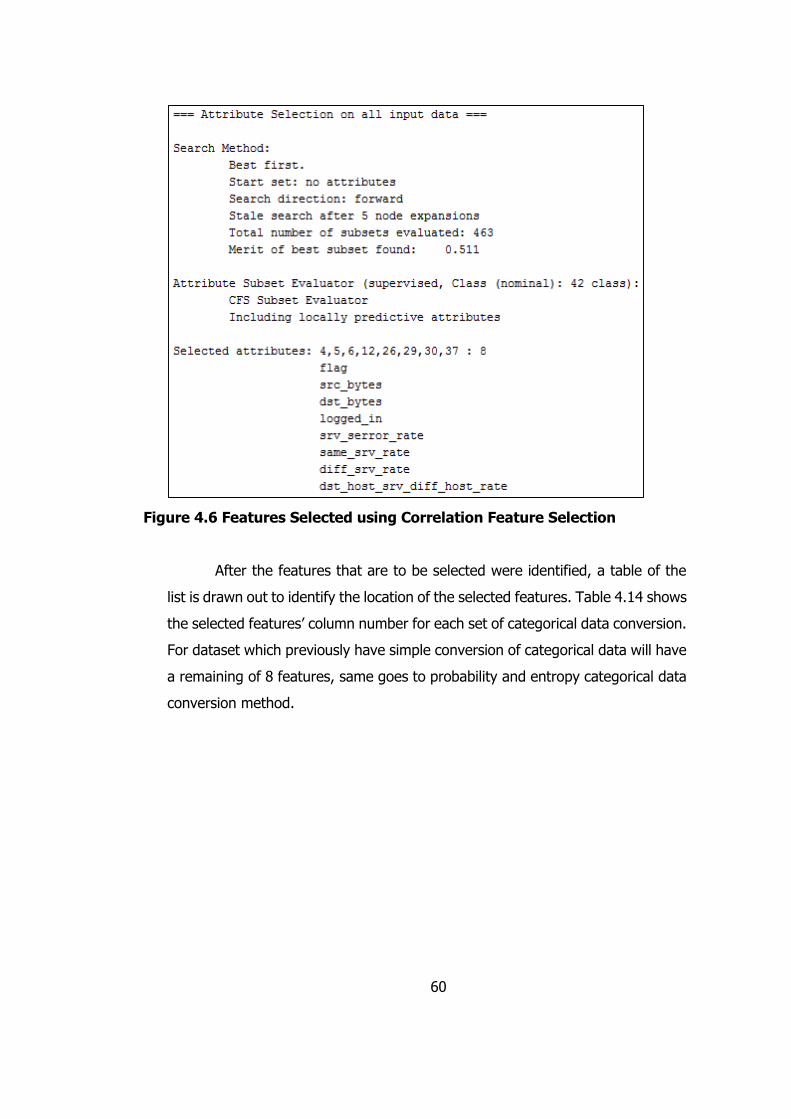
60

Figure 4.6 Features Selected using Correlation Feature Selection

After the features that are to be selected were identified, a table of the

list is drawn out to identify the location of the selected features. Table 4.14 shows

the selected features’ column number for each set of categorical data conversion.

For dataset which previously have simple conversion of categorical data will have

a remaining of 8 features, same goes to probability and entropy categorical data

conversion method.

61

Table 4.14 Selected Features and Their Respective Column for Each Data

Conversion Techniques Colu

mn

Features

Sele

cted

Featu

res

Colu

mn

Features

Sele

cted

Featu

res

1 duration 22 is_guest_login

2 protocol_type 23 count

3 service 24 srv_count

4 flag 4 25 serror_rate

5 src_bytes 5 26 srv_serror_rate 26

6 dst_bytes 6 27 rerror_rate

7 land 28 srv_rerror_rate

8 wrong_fragment 29 same_srv_rate 29

9 urgent 30 diff_srv_rate 30

10 hot 31 srv_diff_host_rate

11 num_failed_logins 32 dst_host_count

12 logged_in 12 33 dst_host_srv_count

13 num_compromised 34 dst_host_same_srv_rate

14 root_shell 35 dst_host_diff_srv_rate

15 su_attempted 36 dst_host_same_src_port_rate

16 num_root 37 dst_host_srv_diff_host_rate 37

17 num_file_creations 38 dst_host_serror_rate

18 num_shells 39 dst_host_srv_serror_rate

19 num_access_files 40 dst_host_rerror_rate

20 num_outbound_cmds 41 dst_host_srv_rerror_rate

21 is_host_login 42 class

4.3 Experimental Setting

Previous section discusses how all the data being pre-processed for experiments,

whereas in this is section, details about experiments carried in this research are

stated clearly. After the data is successfully represented in a point series format, the

data is then separated into ten smaller sets to perform 10-fold cross validation. Each

set contains 14851 of data entries except for last test set which contains a total of

14857 data entries. A total of four set experiments was carried out in realizing the

objectives of this research paper.

62

4.3.1 Experiment I: No Categorical Data

The main objective of performing Experiment I is to provide a benchmark for

comparison for following experiments. We must first know categorical data affects

the classification thus categorical features “protocol_type”, “service” and “flag” were

first remove from the dataset. K-Nearest Neighbour with three different similarity

measure will be performed to classify the network activities, they are the Euclidean

Distance, Cosine Similarity and also Dynamic Time Warping. The K-Nearest

Neighbour classification method is also repeated using different value of k where k=1,

3, 5 …19. The result obtained from this experiment serve as a baseline for

comparison.

4.3.2 Experiment II: Simple Conversion

First method used for the conversion of categorical data is the simple conversion

techniques that were discussed in Section 4.2.1 (a). This method is chosen as the

Experiment II for it is the most common categorical data conversion technique found

in the literature. Again, K-Nearest Neighbour (K-NN) with three different similarity

measure will be performed to classify the network activities. The K-NN classification

method is also repeated using different value of k, where top three k (k=1, 3 and 5)

value that yields the best performance in terms of average accuracy, sensitivity and

specificity in Experiment I are selected. Result from this experiment serves as the

second baseline.

4.3.3 Experiment III: Probability and Entropy Conversion

In Experiment III, classification of network traffic activities is performed on dataset

which have undergone probability and entropy conversion [discussed previously in

4.2.1 (b) & (c)]. Best two similarity measure (Euclidean Distance and Cosine Similarity)

of K-Nearest Neighbour (K-NN) in 4.3.2 are selected to perform classification in

Experiment III, like previous experiments, K-NN classification algorithm is repeated

by selecting the best three values of k (k=1, 3 and 5).

63

4.3.4 Experiment IV: Feature Selection using Information Gain and

Correlation Feature Selection

Last set of experiment involves in identifying the feature selection techniques that

are able to reduce the data dimension of the dataset. Feature Selection method used

in this research are the Information Gain and the Correlation Features Selection

(4.2.3). K-Nearest Neighbour is then applied to the data to classify the network traffic

activities.

Results from the above experiments are properly recorded for analysis purpose in

the next chapter. The results obtained will also be used to compare with the

performance of other machine learning techniques stated in the literature.

4.4 Summary

This chapter aims to provide readers on the steps taken before and during the

experiment. The data must be prepared or rather pre-processed before it can be

loaded to carry out the experiment. Three important steps were carried out in the

data pre-processing phase, which are the conversion of categorical data, data

normalization and lastly feature selection. Conversion of categorical data into numeric

value is accomplished using three conversion technique, namely, Alphabetical Simple

Conversion, Probability Conversion and Entropy Conversion. The converted data were

then combined with the rest of numerical data and further normalized using the min-

max normalization method. K-NN classification with three similarity measure,

Euclidean distance, Cosine Similarity and Dynamic Time Warping were performed on

the data above. The data were also later undergo feature selection method to reduce

the data dimensionality. As the involved dataset is very huge, the process is thus

cumbersome.

CHAPTER 5

RESULLT AND ANALYSIS

5.1 Chapter Overview

In this chapter, the result and analysis of experiments that were performed in the

previous chapter are stated. Comparison of the performance of each experiment will

be explained in detail. Section 5.2 shows the result and analysis for Experiment I,

whereas Section 5.3 discuss the result obtained from Experiment II and its

corresponding analysis. In Section 5.4, analysis is based on the result obtained from

the Experiment III. Section 5.5 discuss about the result from Experiment IV. In

section 5.6, comparison is made between the obtained results and related works

identified in the literature review.

5.2 Experiment I: No Categorical Data

In Experiment I, categorical data are being removed from both of the test set and

train set. K-Nearest Neighbour (K-NN) Classification with Euclidean Distance, Cosine

Similarity and Dynamic Time Warping were performed. For the first experiment,

Euclidean Distance is used as the distance similarity measure in K-NN. The

experiments were also repeated using different number of k, ranging from K = 1, 3,

5, 7, 9, 11 … 19. Table 5.1 below shows the average accuracy, sensitivity and

specificity and the corresponding standard deviation when performing Euclidean

Distance (ED) as the distance similarity measure with no categorical data present in

the dataset.

65

Table 5.1 Result of K-NN with ED on Dataset with No Categorical

Features

Euclidean No Categorical Conversion

K accuracy sensitivity specificity

Average Std dev Average Std dev Average Std dev

1 98.66 0.12 98.61 0.14 98.72 0.14

3 98.58 0.28 98.50 0.46 98.67 0.46

5 98.60 0.13 98.50 0.12 98.71 0.12

7 98.51 0.16 98.42 0.14 98.61 0.14

9 98.46 0.15 98.41 0.12 98.50 0.12

11 98.36 0.16 98.32 0.11 98.41 0.11

13 98.27 0.18 98.23 0.14 98.33 0.14

15 98.22 0.18 98.20 0.16 98.25 0.16

17 98.17 0.20 98.16 0.17 98.18 0.17

19 98.11 0.23 98.12 0.14 98.11 0.14

From Table 5.1, it is clearly seen that the best three K value equals to 1, 3

and 5 for K-NN with ED. With K value equals to 1, the K-NN achieved an average

accuracy of 98.66%. For the sensitivity, an average of 98.61% score is recorded and

a score of 98.72% of average specificity is recorded. When K is equal to 5, the

average accuracy achieved a score of 98.60%, 98.50% for average sensitivity and

average specificity of 98.71% making its performance slightly worse than that of k=1.

When K=3, the performance of K-NN with ED performed the third best with average

accuracy of 98.58%, average sensitivity of 98.50% and 98.67% for average

specificity.

For the second experiment, Cosine Similarity is used as the distance similarity

measure in K-NN. The experiments were also repeated using different number of k,

ranging from K = 1, 3, 5, 7, 9, 11 … 19. Table 5.2 below shows the average accuracy,

sensitivity and specificity and the corresponding standard deviation when performing

Cosine Similarity as the distance similarity measure with no categorical data present

in the dataset.

66

Table 5.2 Result of K-NN with Cosine on Dataset with No Categorical

Features

Cosine No Categorical Conversion

K Accuracy Sensitivity Specificity

Average Std dev Average Std dev Average Std dev

1 98.67 0.08 98.63 0.13 98.71 0.12

3 98.66 0.06 98.56 0.13 98.77 0.09

5 98.63 0.08 98.52 0.13 98.75 0.12

7 98.53 0.10 98.43 0.15 98.63 0.16

9 98.47 0.10 98.43 0.13 98.52 0.13

11 98.38 0.09 98.34 0.15 98.43 0.13

13 98.31 0.11 98.25 0.17 98.38 0.15

15 98.26 0.12 98.21 0.20 98.31 0.15

17 98.18 0.12 98.14 0.19 98.23 0.16

19 98.14 0.14 98.10 0.20 98.18 0.16

From Table 5.2, the best three K value equals to 1, 3 and 5 for K-NN with

Cosine. With K value equals to 1, the K-NN achieved an average accuracy of 98.67%.

For the sensitivity, an average of 98.63% score is recorded and a score of 98.71%

of average specificity is recorded. When K is equal to 3, the average accuracy

achieved a score of 98.66%, 98.56% for average sensitivity and average specificity

of 98.77% making its performance slightly worse than that of K=1. When K=5, the

performance of K-NN with Cosine performed the third best with average accuracy of

98.63%, average sensitivity of 98.52% and 98.75% for average specificity.

Table 5.3 Result of K-NN with DTW on Dataset with No Categorical

Features

DTW - No Categorical Features

K Accuracy Sensitivity Specificity

Average Std dev Average Std dev Average Std dev

1 98.96 0.36 98.90 0.30 99.01 0.50

3 98.58 0.36 98.50 0.28 98.67 0.46

Table 5.3 shows the result obtained from the experiment which perform K-NN with

DTW. From table 5.3, the classification of KNN-DTW have the best performance,

achieving a score of 98.96% for accuracy, 98.90% for sensitivity and specificity of

67

99.01% when k=1. Meanwhile, when k=3, accuracy of 98.58% is recorded,

sensitivity of 98.50% and 98.67% for specificity.

Note that in this experiment only K = 1 and 3 is used. This is due to the time

constraint exist in performing the classification using Dynamic Time Warping for K-

Nearest Neighbour. Furthermore, previous experiments provide experience on the

trend of K, where K performs the best when is equal to one. Thus, the classification

of KNN–DTW stops at K=3. Following experiments which involved KNN-DTW are also

performed in similar fashion.

5.3 Experiment II: Simple Conversion

In Experiment II, the categorical data is being converted to numerical data using the

simple conversion method. K-Nearest Neighbour (K-NN) Classification with Euclidean

Distance, Cosine Similarity and Dynamic Time Warping were performed. The

experiments were repeated using different number of k where k = 1, 3, 5 [three k

values that have the best performance on previous section]. Table 5.4, 5.5 and 5.6

below shows the average accuracy, sensitivity and specificity and the corresponding

standard deviation when performing Euclidean Distance (ED), Cosine Similarity and

Dynamic Time Warping as the distance similarity measure with simple converted

categorical data present in the dataset.

Table 5.4 Result of K-NN with ED on Dataset with Simple Conversion on

Categorical Features

Euclidean Simple Categorical Conversion - Full Features

N Accuracy Sensitivity Specificity

Average Std dev Average Std dev Average Std dev

1 97.97 0.21 97.99 0.13 97.94 0.13

3 97.87 0.17 97.90 0.16 97.84 0.16

5 97.78 0.22 97.90 0.19 97.66 0.19

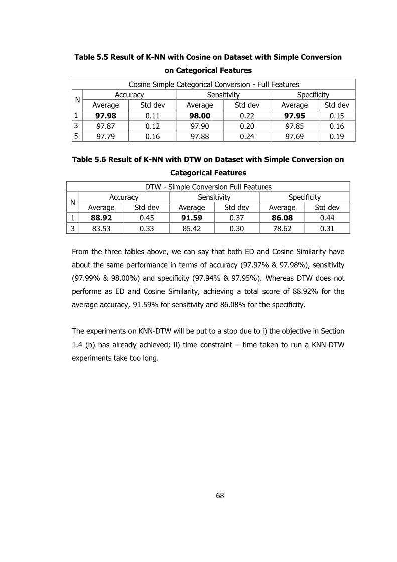
68

Table 5.5 Result of K-NN with Cosine on Dataset with Simple Conversion

on Categorical Features

Cosine Simple Categorical Conversion - Full Features

N Accuracy Sensitivity Specificity

Average Std dev Average Std dev Average Std dev

1 97.98 0.11 98.00 0.22 97.95 0.15

3 97.87 0.12 97.90 0.20 97.85 0.16

5 97.79 0.16 97.88 0.24 97.69 0.19

Table 5.6 Result of K-NN with DTW on Dataset with Simple Conversion on

Categorical Features

DTW - Simple Conversion Full Features

N Accuracy Sensitivity Specificity

Average Std dev Average Std dev Average Std dev

1 88.92 0.45 91.59 0.37 86.08 0.44

3 83.53 0.33 85.42 0.30 78.62 0.31

From the three tables above, we can say that both ED and Cosine Similarity have

about the same performance in terms of accuracy (97.97% & 97.98%), sensitivity

(97.99% & 98.00%) and specificity (97.94% & 97.95%). Whereas DTW does not

performe as ED and Cosine Similarity, achieving a total score of 88.92% for the

average accuracy, 91.59% for sensitivity and 86.08% for the specificity.

The experiments on KNN-DTW will be put to a stop due to i) the objective in Section

1.4 (b) has already achieved; ii) time constraint – time taken to run a KNN-DTW

experiments take too long.

69

5.4 Experiment III: Probability and Entropy Conversion

In Experiment III, classification of K-Nearest Neighbour on dataset which two

proposed categorical data conversion technique which is the probability conversion

and the entropy conversion technique is used (Table 5.7 – Table 5.10).

Table 5.7 Result of KNN-ED on Dataset with Probability Conversion on

Categorical Features

KNN-ED Probability Conversion - Full Features

N Accuracy Sensitivity Specificity

Average Std dev Average Std dev Average Std dev

1 92.25 9.29 92.40 6.74 90.37 10.78

3 91.82 8.99 89.92 14.61 88.58 11.21

5 92.14 8.87 89.94 15.44 88.30 11.00

Table 5.8 Result of KNN-ED on Dataset with Entropy Conversion on

Categorical Features

KNN-ED Entropy Conversion – Full Features

N Accuracy Sensitivity Specificity

Average Std dev Average Std dev Average Std dev

1 99.19 0.04 99.16 0.08 99.22 0.08

3 99.12 0.05 99.13 0.08 99.12 0.10

5 99.03 0.06 99.09 0.09 98.96 0.09

Table 5.9 Result of KNN-Cosine on Dataset with Probability Conversion

on Categorical Features

KNN-Cosine Probability Conversion - Full Features

N Accuracy Sensitivity Specificity

Average Std dev Average Std dev Average Std dev

1 92.28 9.43 92.49 6.63 90.26 11.10

3 91.94 9.10 90.20 14.42 88.55 11.38

5 92.12 9.05 90.19 15.06 88.21 11.21

70

Table 5.10 Result of KNN-Cosine on Dataset with Entropy Conversion on

Categorical Features

KNN-Cosine Entropy Conversion – Full Features

N Accuracy Sensitivity Specificity

Average Std dev Average Std dev Average Std dev

1 99.21 0.05 99.18 0.09 99.24 0.09

3 99.12 0.04 99.12 0.09 99.12 0.09

5 99.02 0.04 99.07 0.09 98.97 0.08

By using the proposed entropy conversion technique, the performance of

classification using both the KNN-ED and KNN-Cosine has increased in all aspects.

Accuracy, sensitivity and specificity of using simple conversion technique mark a

score of around 97.9% where entropy conversion achieves a score of around about

99.3%. This is because by calculating the entropy of the value within a feature, the

ranking between them is conserved. Whereas, if using the simple conversion

technique where the distinct value is arranged alphabetically and further assigned to

a sequence of integer does not conserve the ranking within them. Conversion using

probability conversion technique shows a weaker performance of around 91%.

5.5 Experiment IV: Feature Selection using Information Gain and

Correlation Feature Selection

In this section, only the result of classification using K-NN with Euclidean Distance on

binaurally converted dataset is shown for it has the best performance amongst other

approach mentioned in the previous section.

71

Table 5.11 Result of KNN-ED on Dataset with Reduced Features using

Information Gain =70% Feature Selection and Entropy Conversion on

Categorical Features

Ent-IG- 70%

K Accuracy Sensitivity Specificity

Average Std dev Average Std dev Average Std dev

1 99.16 0.04 99.11 0.09 99.21 0.08

3 99.08 0.05 99.06 0.11 99.10 0.09

5 98.99 0.06 99.02 0.11 98.95 0.09

Table 5.12 Result of KNN-ED on Dataset with Reduced Features using

Information Gain =60% Feature Selection and Entropy Conversion on

Categorical Features

Ent-IG- 60%

K Accuracy Sensitivity Specificity

Average Std dev Average Std dev Average Std dev

1 99.02 0.06 98.96 0.11 99.08 0.07

3 98.91 0.07 98.88 0.12 98.94 0.07

5 98.81 0.07 98.82 0.12 98.79 0.10

Table 5.13 Result of KNN-ED on Dataset with Reduced Features using

Information Gain =50% Feature Selection and Entropy Conversion on

Categorical Features

Ent-IG- 50%

K Accuracy Sensitivity Specificity

Average Std dev Average Std dev Average Std dev

1 98.94 0.05 98.87 0.07 99.00 0.07

3 98.84 0.08 98.81 0.12 98.87 0.11

5 98.72 0.09 98.75 0.14 98.69 0.12

72

Table 5.14 Result of KNN-ED on Dataset with Reduced Features using

Information Gain =40% Feature Selection and Entropy Conversion on

Categorical Features

Ent-IG- 40%

K Accuracy Sensitivity Specificity

Average Std dev Average Std dev Average Std dev

1 98.61 0.12 98.61 0.16 98.61 0.15

3 98.57 0.11 98.50 0.16 98.66 0.14

5 98.52 0.12 98.46 0.18 98.58 0.16

Table 5.15 Result of KNN-ED on Dataset with Reduced Features using

Information Gain =30% Feature Selection and Entropy Conversion on

Categorical Features

Ent-IG- 30%

K Accuracy Sensitivity Specificity

Average Std dev Average Std dev Average Std dev

1 98.21 0.10 98.22 0.16 98.19 0.09

3 98.21 0.10 98.26 0.15 98.16 0.12

5 98.19 0.11 98.32 0.17 98.06 0.16

Table 5.16 Result of KNN-ED on Dataset with Reduced Features using

Correlation Feature Selection and Entropy Conversion on Categorical

Features

Ent-CFS: 8 features

K Accuracy Sensitivity Specificity

Average Std dev Average Std dev Average Std dev

1 94.08 0.84 97.09 2.08 90.83 0.56

3 91.94 0.78 91.89 2.09 92.00 0.72

5 91.94 0.78 91.92 2.10 91.96 0.72

Using Information Gain Features Selection techniques, 5 sets of experiments were

derived with 70%, 60%, …, 30% of total features selected. The results are shown in

Table 5.11 until Table 5.15. The performance of KNN-ED is the best when features

selected are 70% of the total features. Whereas a total of 8 features is selected using

the Correlation Feature Selection technique (Table 5.16). The performance are as

follow, 94.08% for accuracy, 97.09% for sensitivity and specificity of 90.83%.

73

After experiment IV, the performance of feature selection method is evaluated, it is

clearly seen that the performance of the KNN-ED classifier degrade if feature

selection is performed on the data.

5.6 Comparison of Performance of Network Traffic Classifier with other

Machine Learning Approach

Panda et al., 2010 apply discriminative multinomial Naïve Bayes with various filtering

analysis to build a network intrusion detection system. Table 5.17 below shows the

results of the proposed algorithm.

Table 5.17 Results for Various Algorithms

Classifier Detection Accuracy (%) False Alarm Rate in %

Discriminative Multinomial Naïve Bayes + PCA

94.84 4.4

Discriminative Multinomial Naïve Bayes + RP

81.47 12.85

Discriminative Multinomial Naïve Bayes + N2B

96.5 3.0

Table 5.18 Result for Application of SOM-ANN Algorithms

Classifier Successful Detection Rate (%)

SOM 68.88

In the research paper by (Ibrahim et al., 2013), Self-Organization Map (SOM)

Artificial Neural Network (ANN) is performed on the intrusion database (KDD99 and

NSL-KDD). Table 5.18 above shows the result for the application of SOM-ANN

Algorithms.

Compared machine learning methods are Discriminative Multinomial Naïve

Bayes (DMNB), Self-Organization Map (SOM) Artificial Neural Network (ANN) and K-

Nearest Neighbour algorithm with Euclidean Distance as the distance similarity

measure (Table 5.19). Using the same data set, 1NN-ED Entropy Conversion has the

best performance ~99% as compared to DMNB + PCA (94.84%) and DMNB + N2B

74

(96.5%) in terms of accuracy. The other conversion techniques – probability

conversion however, have a weaker performance 92.24%, but still manage to

outperform DMNB+RP (81.47%). In terms of false alarm rate, 1NN-ED Entropy

Conversion also outperformed the rest machine learning approach having the lowest

value of 0.84%. As far as sensitivity is concerned, the 1NN-ED Entropy Conversion

also has the best performance (99.22%). Categorical data that are converted into

numeric value using the Entropy conversion method conserved the ranking within

them thus showing such good performance.

Table 5.19 Comparison of the Performance of Proposed Method and

Other Machine Learning

5.7 Chapter Summary

This chapter shows the tabulation of the result of each experiment. We can conclude

that using different conversion technique to convert categorical data yields different

results. Form the experiment, using full features with the Entropy conversion of the

dataset does provide the best performance of classifier. The performance of

Euclidean distance as a distance similarity measure for K-Nearest Neighbour

algorithm are the best in terms of accuracy, sensitivity and specificity and also the

time taken to classify a network traffic data.

Classifier Accuracy / Detection

Accuracy (%)

False Alarm Rate (%)

Sensitivity / Detection Rate

(%)

Discriminative Multinomial Naïve Bayes + PCA

94.84 4.4

Discriminative Multinomial Naïve Bayes + RP

81.47 12.85

Discriminative Multinomial Naïve Bayes + N2B

96.5 3.0

SOM-ANN 68.88

1NN-ED Entropy Conversion (Proposed)

99.19 0.84 99.22

1NN-ED Probability Conversion (Proposed)

92.24 7.6 90.37

CHAPTER 6

CONCLUSION

6.1 Chapter Overview

This chapter summaries the whole research paper by revising the problem

background, the research’ objectives. Discussion is also on the summary of the

literature review. An outline will also be given to the proposed methodology.

6.2 Summary of Research Paper

The evolving of new types of attacks and virus has urged the need for the emergence

of strong Intrusion Detection System (IDS). IDS that is anomaly-based detection

requires strong algorithm that is fast and cost saving in terms of computational

complexity. Thus, it arises the problem, “Is TSC feasible to classify activities of

network traffic in particular to IDS?” This research is carried out to answer the

question by identifying (i) What are the features that can be extracted from network

traffic to generate Point Series Data? And (ii.) How can the TSC technique best tuned

to detect intrusion on network data?

This research paper focus on the application of Time Series Classification

(TSC) technique to classify network activities so as to detect anomaly. K-Nearest

Neighbour Algorithm (k-NN) is performed to classify the network traffic activities and

subsequently, Dynamic Time Warping algorithm, one of the TSA technique is used

as the similarity measure of the k-NN algorithm.

In the Literature Review of Chapter 2, Introduction of IDS is discussed and

the application of DTW as one of the TSC techniques is also reviewed. Importance

76

of data pre-processing is discussed, including the conversion of symbolic features

and feature selection. The k-NN algorithm is also discussed here.

As for Chapter 3, the methodology that will be used for this research paper is

being discussed. The research program of work which outline the two phases, Phase

the identification of the best approach to solve the problem “How to represent

network traffic data into point series form” and Phase 2, comparison of the TSC

approach identified in Phase 1 with other approaches found in the literature review.

Three measurements which are the detection rate, false positive rate and also the

accuracy will be used to measure the performance of output.

In chapter 4, a detail explanation on how the experiment will be carried out

to achieve the objective of this research paper. Before starting the experiment, the

data must undergo pre-processing, conversion of data from nominal to numeric is

followed by data normalization. The normalized and converted data will then

undergone feature selection.

Chapter 5 discuss about the result obtained from the experiment. Discussion

on the performance of the result is also done.

Chapter 6 concludes everything that has been done in this research paper. A

summarize table on work done to achieve the objective is also drawn to provide an

easier understanding to the reader.

77

Table 6.1 Work Done to Achieve the Objectives

Objectives Work done

1 To investigate and identify feature transformation technique that can generate point series data for network activities classification

Three different techniques of categorical data features into numeric data is performed which is by using the simple conversion, probability conversion and entropy conversion. Refer Chapter 4.2.1, 5.3 and 5.4 for more details. Feature selection using Information Gain and Correlation Feature Selection Refer Chapter 4.2.3, 5.5 for more details.

2 To investigate the feasibility of Time Series Classification techniques by using k-NN coupled with DTW to classify network traffic activities

Experiment by using DTW as a distance similarity measure for KNN is carried out. Refer Chapter 4.2.1, 5.2 and 5.3 for more details.

3 To investigate the effects of using different similarities measurement, Euclidean Distance (ED) and Cosine similarity algorithm

Various set of experiments is carried out to determine the results of using different distance similarity measures. Refer Chapter 5.2, 5.3 and 5.4 for more details.

4 To compare the performance of network traffic classifier produced in (b) and (c) with other machine learning techniques, Self-Organization Map (SOM) Artificial Neural Network (ANN) by (Ibrahim, Basheer, and Mahmod, 2013) and Discriminative Multinomial Naive Bayes (NB) proposed by (Panda, Abraham, and Patra, 2010)

After all the experiments have been carried out, the result is tabulated and take to compare with other machine learning methods in the literature review. Refer Chapter 5.6 for more details.

6.3 Future Works

In this research paper three experiments were performed on the Dynamic Time

Warping distance similarity measure. Due to time and computational constraints,

DTW was not further explored. Future works might include the tuning on the

algorithm of DTW to enable fast computation. Besides, the proposed probability

conversion can be further explored to convert categorical data.

REFERENCES

Amr, T. (2012). Survey on Time-Series Data Classification, 1–10.

Anderson, J. P. (1980). Computer Security Threat Monitoring and Surveillance.

Apple confirms accounts compromised but denies security breach. (2014, September 2). BBC. Retrieved from http://www.bbc.com/news/technology-29011850

Bouzida, Y., & Cuppens, F. (2004). Efficient intrusion detection using principal component analysis. Proceedings of the. Retrieved from http://yacine.bouzida.free.fr/Articles/2004SAR.pdf

Brockwell, P. J., & Davis, R. A. (2002). Introduction to Time Series and Forecasting , Second Edition Springer Texts in Statistics.

Chaovalitwongse, W. A., Fan, Y., & Sachdeo, R. C. (2007). On the Time Series <formula formulatype=“inline”><tex>$K$</tex></formula>-Nearest Neighbor Classification of Abnormal Brain Activity. IEEE Transactions on Systems, Man, and Cybernetics - Part A: Systems and Humans, 37(6), 1005–1016. doi:10.1109/TSMCA.2007.897589

Chowdhary, M., Suri, S., & Bhutani, M. (2014). Comparative Study of Intrusion Detection System. International Journal of Computer Sciences and Engineering, 2(4), 197–200.

Datti, R., & Verma, B. (2010). Feature Reduction for Intrusion Detection Using Linear Discriminant Analysis. International Journal on Computer Science and Engineering (IJCSE), 02(04), 1072–1078.

Davis, J. J., & Clark, A. J. (2011). Data preprocessing for anomaly based network intrusion detection: A review. Computers & Security, 30(6-7), 353–375. doi:10.1016/j.cose.2011.05.008

Deepa, a. J., & Kavitha, V. (2012). A Comprehensive Survey on Approaches to Intrusion Detection System. Procedia Engineering, 38, 2063–2069. doi:10.1016/j.proeng.2012.06.248

Elsayed, A., Hijazi, M. H. A., Coenen, F., Garc´ıa-Fi˜Nana˜, M., Sluming, V., & Zheng, Y. (2011). Time Series Case Based Reasoning for Image Categorisation. In Case-Based Peasoning Research and Development (pp. 423–436). doi:10.1007/978-3-642-23291-6_31

García-Teodoro, P., Díaz-Verdejo, J., Maciá-Fernández, G., & Vázquez, E. (2009). Anomaly-based network intrusion detection: Techniques, systems and challenges. Computers & Security, 28(1-2), 18–28. doi:10.1016/j.cose.2008.08.003

79

Gillian, N., Knapp, R. B., & Modhrain, S. O. (2011). Recognition Of Multivariate Temporal Musical Gestures Using N-Dimensional Dynamic Time Warping, (June), 337–342.

He, W., Hu, G., Yao, X., Gangyuan, K., Wang, H., & Hongmei, X. (2008). Applying multiple time series data mining to large-scale network traffic analysis. 2008 IEEE Conference on Cybernetics and Intelligent Systems, 394–399. doi:10.1109/ICCIS.2008.4670844

Hernández-Pereira, E., Suárez-Romero, J. a., Fontenla-Romero, O., & Alonso-Betanzos, a. (2009). Conversion methods for symbolic features: A comparison applied to an intrusion detection problem. Expert Systems with Applications, 36(7), 10612–10617. doi:10.1016/j.eswa.2009.02.054

Ibrahim, L. M., Basheer, D. T., & Mahmod, M. S. (2013). A Comparison Study for Intrusion Database (KDD99, NSL-KDD) Based on Self Organization Map(SOM) Artificial Neural Network. Journal of Engineering Sience and Technology, 8(1), 107–119.

Karagiannis, T., Papagiannaki, K., & Faloutsos, M. (2005). BLINC : Multilevel Traffic Classification in the Dark. In ACM SIGCOMM Conference 2005 (pp. 229–240). ACM.

Kia, A., SamanHaratizadeh, & HadiZare. (2013). Prediction of USD / JPY Exchange Rate Time Series Directional Status by KNN with Dynamic Time. Bonfring International Journal of Data Mining, 3(2), 12–16. doi:10.9756/BIJDM.4658

Kumar, S. (2007). Survey of Current Network Intrusion Detection Techniques. Citeseer, 1–18. Retrieved from http://citeseerx.ist.psu.edu/viewdoc/download?doi=10.1.1.129.7105&rep=rep1&type=pdf\npapers2://publication/uuid/42BBD57C-EACC-4349-AC44-F69CDF10E018

Li, H., Chen, C. L. P., & Huang, H.-P. (2000). Fuzzy Neural Intelligent Systems: Mathematical Foundation and the Applications in Engineering. Taylor & Francis. Retrieved from https://books.google.com/books?id=IzvqngEACAAJ&pgis=1

More, S., Matthews, M., Joshi, A., & Finin, T. (2012). A knowledge-based approach to intrusion detection modeling. Proceedings - IEEE CS Security and Privacy Workshops, SPW 2012, 75–81. doi:10.1109/SPW.2012.26

Muscillo, R., Schmid, M., Conforto, S., & D’Alessio, T. (2011). Early recognition of upper limb motor tasks through accelerometers: real-time implementation of a DTW-based algorithm. Computers in Biology and Medicine, 41(3), 164–72. doi:10.1016/j.compbiomed.2011.01.007

Panda, M., Abraham, A., & Patra, M. (2010). Discriminative multinomial naive bayes for network intrusion detection. In 2010 Sixth International Conference on

80

Information Assurance and Security (IAS) (pp. 5–10). Retrieved from http://ieeexplore.ieee.org/xpls/abs_all.jsp?arnumber=5604193

Robbins, R. (2002). Distributed Intrusion Detection Systems: An Introduction and Review.

Roobaert, D., Karakoulas, G., & Chawla, N. V. (2006). Information gain, correlation and support vector machines. Retrieved June 21, 2015, from http://www.springerlink.com/index/KJ45153333192803.pdf

Sabahi, F., & Movaghar, a. (2008). Intrusion Detection: A Survey. 2008 Third International Conference on Systems and Networks Communications, 23–26. doi:10.1109/ICSNC.2008.44

Shyu, M.-L., Chen, S.-C., Sarinnapakorn, K., & Chang, L. (2003). A Novel Anomaly Detection Scheme Based on Principal Component Classifier. Retrieved from http://oai.dtic.mil/oai/oai?verb=getRecord&metadataPrefix=html&identifier=ADA465712\nhttp://www.dtic.mil/cgi-bin/GetTRDoc?Location=U2&doc=GetTRDoc.pdf&AD=ADA465712

Stolfo, S. J., Fan, W., Lee, W., Prodromidis, A., Street, W., York, N., & Chan, P. K. (1999). Cost-based Modeling and Evaluation for Data Mining With Application to Fraud and Intrusion Detection : Results from the JAM Project ∗.

Tavallaee, M., Bagheri, E., Lu, W., & Ghorbani, A. a. (2009). A detailed analysis of the KDD CUP 99 data set. 2009 IEEE Symposium on Computational Intelligence for Security and Defense Applications, (Cisda), 1–6. doi:10.1109/CISDA.2009.5356528

Wang, W., & Battiti, R. (2006). Identifying intrusions in computer networks with principal component analysis. Proceedings - First International Conference on Availability, Reliability and Security, ARES 2006, 2006, 270–277. doi:10.1109/ARES.2006.73

Weller-Fahy, D., Borghetti, B., & Sodemann, A. (2014). A Survey of Distance and Similarity Measures used within Network Intrusion Anomaly Detection. IEEE Communications Surveys & Tutorials, PP(99), 1–1. doi:10.1109/COMST.2014.2336610

Wu, X., Kumar, V., Quinlan, J. R., Ghosh, J., Yang, Q., Motoda, H., … Dan, J. H. (2008). Top 10 algorithms in data mining. doi:10.1007/s10115-007-0114-2

Xu, X. (2006). Adaptive intrusion detection based on machine learning: Feature extraction, classifier construction and sequential pattern prediction. International Journal of Web Services Practices, 2(1), 49–58. Retrieved from http://citeseerx.ist.psu.edu/viewdoc/download?doi=10.1.1.107.9575&rep=rep1&type=pdf