Effects of Long-Term Creep on the Integrity of Modern Wood Structures

by

Jacem Tissaoui

Dissertation submitted to the Faculty of the

Virginia Polytechnic Institute and State University

in partial fulfillment of the requirements for the degree of

Doctor of Philosophy

in

Civil Engineering

Approved:

Siegfried M. Holzer, Co-Chair Joseph R. Loferski, Co-Chair

David A. Dillard Surot Thangjitham

Don A. Garst

December, 1996

Blacksburg, Virginia

Keywords: Creep, Wood, Structures, Finite Element, TTSP

Effects of Long Term Creep on the Integrity of Modern Wood Structures

byJacem Tissaoui

S. M. Holzer, Co-ChairmanJ. R. Loferski, Co-Chairman

(ABSTRACT)

Short-term creep tests in tension and in compression were conducted onsouthern pine, Douglas-fir, yellow-poplar, and Parallam™ samples attemperatures ranging between 20 and 80°C and at 6, 9 and 12% moisturecontent. The principle of time-temperature superposition was applied toform a master curve that extended for a maximum of 2 years. The horizontalshift factors followed an Arrhenius relation with activation energies rangingbetween 75 and 130 kJ/mole. It was not possible to superpose the compliancecurves at 70 and 80°C, this is attributed to the presence of multiplecomponents in wood with different temperature dependence.

Long-term creep tests were also conducted in tension and in compression at20°C and 12% moisture content for over 2 years. The resulting compliancecurves were fitted to the power law equation using a nonlinear fittingprocedure. The results were compared with those of the short-term creeptests.

Finite element analysis was conducted on selected wood structures todetermine the effect of creep on serviceability and stability.

iii

Acknowledgments

I am very grateful to Dr. S. M. Holzer for his continued support, encouragement,and guidance. I also thank Dr. J. R. Loferski for serving as Co-Chairman and for hishelp with the experimental part. Thanks are due to Dr. D. A. Dillard for hisvaluable contributions and suggestions. I also thank Dr. S. Thangjitham, Dr. D. A.Garst, and Dr. M. P. Wolcott for serving on my committee and for their helpfulcomments.I thank Dr. R. L. Youngs and Dr. A. A. Trani for their support, and the techniciansespecially Denson Graham and Harold Vandivort for the excellent job they did inmaking the experimental fixtures.I also thank Raul Andruet, Samruam Tongtoe, and Amara Loulizi for theirfriendship and support.Finally I am grateful to my wife Luz and son Yassine for making my life inBlacksburg enjoyable.

iv

Table of Contents

1 . I N T R O D U C T I O N . . . . . . . . . . . . . . . . . . . . . . . . . . . . . . . . . . . . . . . . . . . . . . . . . . . . . . . . . . . . . . . . . . . . . . . . . . . . . . . . . . . . . . . . . . 1

1.1 BACKGROUND ...............................................................................................................................11.2 RESEARCH NEEDS...........................................................................................................................31.3 SCOPE AND OBJECTIVES ..................................................................................................................31.4 SIGNIFICANCE ................................................................................................................................4

2 . L I T E R A T U R E R E V I E W . . . . . . . . . . . . . . . . . . . . . . . . . . . . . . . . . . . . . . . . . . . . . . . . . . . . . . . . . . . . . . . . . . . . . . . . . . . . . . . . . . 5

2.1 GLASS TRANSITION TEMPERATURE OF POLYMERS................................................................................52.2 GLASS TRANSITION TEMPERATURES FOR WOOD...................................................................................72.3 THE PRINCIPLE OF TIME-TEMPERATURE SUPERPOSITION.....................................................................102.4 THE PRINCIPLE OF TIME-MOISTURE SUPERPOSITION..........................................................................132.5 APPLICATION OF TTSP TO WOOD ....................................................................................................202.6 APPLICATION OF TTSP TO THERMORHEOLOGICALLY COMPLEX MATERIALS..........................................212.7 CREEP MODELS ............................................................................................................................242.8 FINITE ELEMENT ANALYSIS FOR CREEP............................................................................................26

2.8.1 Creep Models........................................................................................................................262.8.2 Computer Programs.................................................................................................................302.8.3 Creep Stability.......................................................................................................................302.8.4 Creep Analyses.......................................................................................................................31

3 . E X P E R I M E N T A L . . . . . . . . . . . . . . . . . . . . . . . . . . . . . . . . . . . . . . . . . . . . . . . . . . . . . . . . . . . . . . . . . . . . . . . . . . . . . . . . . . . . . . . . 3 2

3.1 DYNAMIC TESTS USING THE DMA....................................................................................................323.2 SHORT-TERM CREEP TESTS.............................................................................................................323.3 LONG-TERM CREEP TESTS...............................................................................................................41

4 . R E S U L T S . . . . . . . . . . . . . . . . . . . . . . . . . . . . . . . . . . . . . . . . . . . . . . . . . . . . . . . . . . . . . . . . . . . . . . . . . . . . . . . . . . . . . . . . . . . . . . . . . 4 5

4.1 DYNAMIC TESTS ...........................................................................................................................454.1.1 Fixed frequency tests................................................................................................................454.1.2 Creep Tests............................................................................................................................51

4.2 SHORT-TERM CREEP TESTS............................................................................................................524.2.1 Difficulties.............................................................................................................................524.2.2 Creep in tension......................................................................................................................534.2.3 Creep in compression...............................................................................................................624.2.4 Time-moisture superposition creep test........................................................................................74

4.3 LONG-TERM CREEP TESTS..............................................................................................................774.3.1 Creep in tension......................................................................................................................784.3.2 Analytical Criterion for the application of TTSP to wood...............................................................884.3.3 Comparison between short-term and long-term results....................................................................94

4.4 FINITE ELEMENT ANALYSIS............................................................................................................954.4.1 Creep model using time hardening model.....................................................................................954.4.2 Creep model with user subroutine...............................................................................................964.4.3 Incorporation of the creep law from experimental analysis...............................................................974.4.4 Creep analysis checking............................................................................................................984.4.5 Analysis of a truss for creep.....................................................................................................1014.4.6 Finite element analysis for stability...........................................................................................105

5. CONCLUSIONS AND RECOMMENDATIONS . . . . . . . . . . . . . . . . . . . . . . . . . . . . . . . . . . . . . . . . . . . . . . . . . . . 1 1 3

5.1 CONCLUSIONS.............................................................................................................................1135.2 RECOMMENDATIONS....................................................................................................................113

6 . R E F E R E N C E S . . . . . . . . . . . . . . . . . . . . . . . . . . . . . . . . . . . . . . . . . . . . . . . . . . . . . . . . . . . . . . . . . . . . . . . . . . . . . . . . . . . . . . . . . . 1 1 5

v

List Of Illustrations

FIGURE 1.1 (A) CREEP, (B) STRESS RELAXATION, (C) RECOVERY.................................................................2FIGURE 2.1 MODULUS (E) AS A FUNCTION OF TEMPERATURE FOR A TYPICAL AMORPHOUS POLYMER...............6FIGURE 2.2 STORAGE MODULUS (E') FOR MAPLE AND SPRUCE AT 10% MOISTURE CONTENT (KELLY ET AL. 1987)8FIGURE 2.3 LOSS TANGENT (TAN∆) FOR MAPLE AND SPRUCE AT 10% MOISTURE CONTENT (KELLY ET AL. 1987).8FIGURE 2.4 GLASS TRANSITION TEMPERATURES OF IN-SITU LIGNIN (Α1) AND HEMICELLULOSE (Α2) AS A

FUNCTION OF MOISTURE CONTENT (KELLY ET AL. 1987).....................................................................9FIGURE 2.5 CONSTRUCTION OF THE MASTER CURVE FROM EXPERIMENTAL MODULUS CURVES AT VARIOUS

TEMPERATURES (AKLONIS AND MACKNIGHT 1983).........................................................................11FIGURE 2.6 EFFECT OF RELATIVE HUMIDITY AND TEMPERATURE ON RELATIVE CREEP OF UF CHIPBOARD,

PLYWOOD, AND SCOTS PINE.........................................................................................................13FIGURE 2.7 COMPLIANCE CURVES FOR PVAC AT 0% MOISTURE CONTENT AND AT DIFFERENT TEMPERATURES

(EMRI AND PAVSEK, 1992)...........................................................................................................15FIGURE 2.8 MASTER CURVE FROM TTSP FOR PVAC AT 0% MOISTURE CONTENT (EMRI AND PAVSEK, 1992)...16FIGURE 2.9 COMPLIANCE CURVES FOR PVAC AT 20°C AND AT DIFFERENT MOISTURE CONTENTS (EMRI AND

PAVSEK, 1992)...........................................................................................................................17FIGURE 2.10 MASTER CURVE FROM TMSP FOR PVAC AT 20°C (EMRI AND PAVSEK, 1992)...........................18FIGURE 2.11 RELAXATION MODULUS CURVES AT DIFFERENT TEMPERATURES FOR PVA (ONOGI ET AL, 1962)..18FIGURE 2.12 RELAXATION MODULUS CURVES AT DIFFERENT RELATIVE HUMIDITIES FOR PVA (ONOGI ET AL,

1962)........................................................................................................................................19FIGURE 2.13 MASTER CURVE FROM TMSP AT 20°C FOR PVA (ONOGI ET AL, 1962).....................................19FIGURE 2.14 SUPERPOSITION ON THE TIME AXIS FOR THERMORHEOLOGICALLY COMPLEX MATERIALS..........23FIGURE 2.15 SUPERPOSITION ALONG THE TEMPERATURE AXIS..................................................................24FIGURE 2.16 TIME AND STRAIN HARDENING RESPONSES TO VARIABLE STRESS............................................29FIGURE 3.1 TENSION TEST APPARATUS..................................................................................................34FIGURE 3.2 CREEP APPARATUS (A) TENSION, (B) COMPRESSION...............................................................35FIGURE 3.3 LOG TIME AXIS (SECONDS)..................................................................................................37FIGURE 3.4 MECHANICAL CONDITIONING OF SAMPLE 1 AT 25°C................................................................38FIGURE 3.5 MECHANICAL CONDITIONING OF SAMPLE 2 AT 25°C................................................................39FIGURE 3.6 MECHANICAL CONDITIONING OF SAMPLE 3 AT 25°C................................................................40FIGURE 3.7 (A) ACTIVE AND DUMMY SPECIMENS; (B) WHEATSTONE BRIDGE...............................................41FIGURE 3.8 SAMPLE ARRANGEMENT FOR THE LONG-TERM CREEP TESTS.....................................................43FIGURE 3.9 LONG-TERM CREEP TEST SETUP............................................................................................44FIGURE 4.1 LOSS TANGENT FOR PAINTED AND UNPAINTED SOUTHERN PINE SAMPLES...................................46FIGURE 4.2 LOSS TANGENT FOR PAINTED AND UNPAINTED DOUGLAS-FIR SAMPLES......................................47FIGURE 4.3 LOSS TANGENT FOR YELLOW-POPLAR AT 5, 7, AND 9% MOISTURE CONTENTS.............................48FIGURE 4.4 LOSS TANGENT FOR SOUTHERN PINE AT 13.0 AND 9% MOISTURE CONTENTS...............................49FIGURE 4.5 LOSS TANGENT FOR DOUGLAS-FIR AT 12.5 AND 9.5% MOISTURE CONTENTS...............................50FIGURE 4.6 COMPLIANCE CURVES FOR YELLOW-POPLAR AT 5% MOISTURE CONTENT...................................51FIGURE 4.7 COMPLIANCE CURVES FOR YELLOW-POPLAR AT 7% MOISTURE CONTENT...................................52FIGURE 4.8 (A) COMPLIANCE AND (B) MASTER CURVES FOR YELLOW-POPLAR AT 6% MOISTURE CONTENT

(TENSION)..................................................................................................................................55FIGURE 4.9 HORIZONTAL SHIFT FACTORS (TENSION)................................................................................55FIGURE 4.10 MASTER CURVE AND POWER LAW FIT (TENSION)..................................................................56FIGURE 4.11 TEMPERATURE AND RELATIVE HUMIDITY DURING THE TEST....................................................57FIGURE 4.12 COMPLIANCE AND MASTER CURVES FOR SOUTHERN PINE AT 6% MOISTURE CONTENT (TENSION). 57FIGURE 4.13 HORIZONTAL SHIFT FACTORS FOR SOUTHERN PINE, DH=74.6 KJ/MOLE...................................58FIGURE 4.14 COMPLIANCE AND MASTER CURVES FOR YELLOW-POPLAR AT 6% MOISTURE CONTENT (TENSION)59FIGURE 4.15 HORIZONTAL SHIFT FACTORS FOR YELLOW-POPLAR, DH=128.0 KJ/MOLE.................................60FIGURE 4.16 COMPLIANCE AND MASTER CURVES FOR FIRST AT 6% MOISTURE CONTENT (TENSION)...............61FIGURE 4.17 HORIZONTAL SHIFT FACTORS, DH=90.7 KJ/MOLE.................................................................62

vi

FIGURE 4.18 (A) COMPLIANCE AND (B) MASTER CURVES FOR DOUGLAS-FIR AT 9% MOISTURE CONTENT(COMPRESSION).........................................................................................................................64

FIGURE 4.19 HORIZONTAL SHIFT FACTORS (COMPRESSION)......................................................................65FIGURE 4.20 MASTER CURVE AND POWER LAW FIT (COMPRESSION)...........................................................65FIGURE 4.21 TEMPERATURE AND RELATIVE HUMIDITY DURING THE TEST...................................................66FIGURE 4.22 COMPLIANCE AND MASTER CURVES FOR SOUTHERN PINE AT 9% MOISTURE CONTENT

(COMPRESSION).........................................................................................................................67FIGURE 4.23 HORIZONTAL SHIFT FACTORS FOR SOUTHERN PINE AT 9% MOISTURE CONTENT, ∆H = 108.7

KJ/MOLE...................................................................................................................................68FIGURE 4.24 COMPLIANCE AND MASTER CURVES FOR DOUGLAS-FIR AT 9% MOISTURE CONTENT

(COMPRESSION).........................................................................................................................69FIGURE 4.25 HORIZONTAL SHIFT FACTORS FOR DOUGLAS-FIR AT 9% MOISTURE CONTENT, ∆H= 109.0

KJ/MOLE...................................................................................................................................70FIGURE 4.26 COMPLIANCE AND MASTER CURVES FOR PARALLAM™ AT 9% MOISTURE CONTENT

(COMPRESSION).........................................................................................................................71FIGURE 4.27 HORIZONTAL SHIFT FACTORS FOR PARALLAM™ AT 9% MOISTURE CONTENT,...........................72FIGURE 4.28 COMPLIANCE AND MASTER CURVES FOR THE YELLOW-POPLAR SAMPLE...................................74FIGURE 4.29 COMPLIANCE AND MASTER CURVES FOR THE KILN DRIED SOUTHERN YELLOW PINE SAMPLE (MCREF

= 5.21%)...................................................................................................................................75FIGURE 4.30 COMPLIANCE AND MASTER CURVES FOR THE AIR DRIED SOUTHERN YELLOW PINE SAMPLE (MCREF =

5.21%)......................................................................................................................................76FIGURE 4.31 ACTUAL (SYMBOLS) AND POWER LAW FIT (SOLID LINE) FOR THREE SOUTHERN PINE SPECIMENS IN

TENSION....................................................................................................................................78FIGURE 4.32 NORMALIZED COMPLIANCE CURVES FOR THREE SOUTHERN PINE SPECIMENS IN TENSION...........79FIGURE 4.33 ACTUAL (SYMBOLS) AND POWER LAW FIT (SOLID LINE) FOR TWO YELLOW-POPLAR SPECIMENS IN

TENSION....................................................................................................................................80FIGURE 4.34 NORMALIZED COMPLIANCE CURVES FOR TWO YELLOW-POPLAR SPECIMENS IN TENSION............81FIGURE 4.35 ACTUAL (SYMBOLS) AND POWER LAW FIT (SOLID LINE) FOR THREE SOUTHERN PINE SPECIMENS IN

COMPRESSION...........................................................................................................................82FIGURE 4.36 NORMALIZED COMPLIANCE CURVES FOR THREE SOUTHERN PINE SPECIMENS IN COMPRESSION. . .83FIGURE 4.37 ACTUAL (SYMBOLS) AND POWER LAW FIT (SOLID LINE) FOR FOUR YELLOW-POPLAR SPECIMENS IN

COMPRESSION...........................................................................................................................84FIGURE 4.38 NORMALIZED COMPLIANCE CURVES FOR FOUR YELLOW-POPLAR SPECIMENS IN COMPRESSION...85FIGURE 4.39 ACTUAL (SYMBOLS) AND POWER LAW FIT (SOLID LINE) FOR FOUR DOUGLAS-FIR SPECIMENS IN

COMPRESSION...........................................................................................................................86FIGURE 4.40 NORMALIZED COMPLIANCE CURVES FOR FOUR DOUGLAS-FIR SPECIMENS IN COMPRESSION.......87FIGURE 4.41 COMPARISON OF THE LONG-TERM CREEP IN COMPRESSION AND IN TENSION FOR (A) SOUTHERN

PINE AND (B) YELLOW-POPLAR.....................................................................................................88FIGURE 4.42 CREEP CURVES FOR YELLOW-POPLAR IN TENSION AT 9% MOISTURE CONTENT..........................89FIGURE 4.43 FITTED CREEP CURVES FOR YELLOW-POPLAR (TTSP)............................................................90

FIGURE 4.44 d log D

d log t VS. LOG T FOR YELLOW-POPLAR (TTSP).................................................................91

FIGURE 4.45 d log D

d log t VS. LOG T FOR YELLOW-POPLAR (TMSP)................................................................92

FIGURE 4.46 d log D

d log t VS. LOG T (TMSP)..............................................................................................93

FIGURE 4.47 NORMALIZED SHORT-TERM AND LONG-TERM COMPLIANCE CURVES FOR SOUTHERN PINE INCOMPRESSION...........................................................................................................................94

FIGURE 4.48 NORMALIZED SHORT-TERM AND LONG-TERM COMPLIANCE CURVES FOR YELLOW-POPLAR INTENSION....................................................................................................................................95

FIGURE 4.49 ABAQUS AND EXPERIMENTAL RESULTS FOR A TRUSS ELEMENT IN TENSION............................100FIGURE 4.50 ROOF TRUSS...................................................................................................................101FIGURE 4.51 DISPLACEMENT AT MIDDLE OF BOTTOM CHORD...................................................................103

vii

FIGURE 4.52 CREEP DEFLECTION AS A PERCENTAGE OF ELASTIC DEFLECTION............................................104FIGURE 4.53 GEOMETRY OF THE A-FRAME (CROSS SECTIONAL AREA = 1 IN2).............................................105FIGURE 4.54 LOAD DEFLECTION PATH AT THE APEX................................................................................105FIGURE 4.55 LONG TERM RESPONSE OF THE FRAME UNDER 50% OF SHORT TERM CRITICAL LOAD.................106FIGURE 4.56 (A) GEOMETRY AND (B) CROSS SECTION OF THREE HINGED ARCH...........................................108FIGURE 4.57 CREEP DISPLACEMENTS AT THE APEX.................................................................................108FIGURE 4.58 VARAX DOME GEOMETRY.................................................................................................110FIGURE 4.59 BUCKLED SHAPE OF THE DOME..........................................................................................111FIGURE 4.60 VERTICAL DISPLACEMENT AT THE DOME APEX....................................................................112

viii

List of Tables

TABLE 3.1 RELATIVE HUMIDITY REQUIRED TO MAINTAIN A 12% MOISTURE CONTENT..................................36TABLE 3.2 NUMBER OF SAMPLES IN THE LONG-TERM CREEP TEST..............................................................41TABLE 4.1 MOISTURE LOSS DURING FIXED FREQUENCY TEST (25 TO 80°C AT 2°C / MINUTE)..........................45TABLE 4.2 MOISTURE LOSS DURING FIXED FREQUENCY TEST FOR PAINTED SAMPLES (25 TO 80°C AT 2°C /

MINUTE)....................................................................................................................................45TABLE 4.3 POWER LAW PARAMETERS FOR SOUTHERN PINE, YELLOW-POPLAR, AND DOUGLAS-FIR AT 6%

MOISTURE CONTENT IN TENSION...................................................................................................62TABLE 4.4 POWER LAW PARAMETERS FOR SOUTHERN PINE, DOUGLAS-FIR, AND PARALLAM™ AT 6%

MOISTURE CONTENT...................................................................................................................72TABLE 4.5 POWER LAW EQUATION PARAMETERS FOR TENSION FROM LONG-TERM TESTING...........................77TABLE 4.6 POWER LAW EQUATION PARAMETERS FOR COMPRESSION FROM LONG-TERM TESTING..................77TABLE 4.7 CREEP PARAMETERS USED IN FINITE ELEMENT ANALYSIS OF THE VARAX DOME.........................111

11

1. INTRODUCTION

1.1 Background

Viscoelastic materials exhibit properties that are common to both perfectsolids and perfect liquids. As a result, the stress is proportional to the strain,the rate of strain, and possibly higher time derivatives of strain; when thestress is linearly proportional to strain, the material is termed linearlyviscoelastic (Sharma 1965). A constitutive equation for such materials mustcorrectly represent the behavior under well known conditions of stress andstrain. These conditions are creep, stress relaxation, recovery, constant ratestressing, and constant rate straining (Williams 1980). Creep is the continueddeformation under a constant stress while stress relaxation is the reduction instress with time under a prescribed strain. Recovery occurs when the straindecreases as the stress is removed (Figure 1.1).Because wood is a viscoelastic material at normal operating stress,temperature, and moisture content (Van Der Put 1989), it is susceptible tocreep which can lead to serviceability and strength reduction problems.Although the creep behavior of wood has been extensively studied, no long-term creep model (50 years) exists. Current design practices (NDS 1986; AITC1985) account for creep by magnifying the dead load deflections usingempirical factors. Creep in wood structures can lead to serviceabilityproblems due to excessive deformations or to safety problems due to strengthreduction. Modern wood structures such as lattice domes and arches areparticularly prone to instability (snap-through or torsional instability). Long-term creep can lead to instability by magnifying the short-term deflections.

22

time

time

time

time

time

time

stre

ss

stra

in

stre

ssst

ress

stra

in

(a)

stra

in

(b)

(c)

prescribed stress

response

response

prescribed strain

responseprescribed stress

Figure 1.1 (a) creep, (b) stress relaxation, (c) recovery.

33

1.2 Research Needs

As reliability based design replaces traditional design practices, a long-termcreep law for wood becomes necessary to account for the time-dependentbehavior of wood. However, most of the creep data was obtained frombending tests which represent member behavior rather than materialbehavior (Holzer et al. 1989). There is also a lack of information about thelong-term behavior of structural composite lumber. For example, in a reporton creep rupture testing of Parallam™ at MacMillan Bloedel Ltd., Bledsoe etal. (1990) emphasize that static testing alone cannot guarantee the long-timeperformance of composite materials. Two Parallam™ products that wereobtained using different pressing strategies had different creep and creeprupture behavior in spite of their similar modulii of rupture.

Moreover, in the 1991 proceedings of the NATO advanced researchworkshop on reliability-based design of engineered wood structures (Bodig1992), the group on material resistance considerations identified the long-term behavior of structural composite lumber as an area where research isneeded:

"Improvements must be sought in our knowledge of the long-term behavior of non-lumber materials. This information couldhelp improve structural modeling, and also clarify questions ofthe linkages between strength degradation and creep, as well asthe interaction between environmental effects, threshold levelsfor strength, upper limits of creep deformations, etc."

Furthermore, Leichti et al. (1990) cite the lack of information about the long-term behavior and durability of structural wood composites as the mainreason why designers are reluctant to use them in primary structuralapplications.

The principle of time-temperature superposition (TTSP) can be used to obtaina long-term creep law from a series of short-term tests at differenttemperatures. Although the principle has been used for man-madepolymers, very little research has been conducted to investigate itsapplicability to wood.

1.3 Scope and Objectives

The main goal of the study is to investigate the long-term behavior of plane andspatial wood structures. To achieve this goal, the following is needed:

44

1• To determine whether and under what conditions TTSP is valid for wood andwood composites. For this study, two common structural softwoods, southernyellow pine (Pinus spp.) and Douglas-fir (Pseudotsuga menziesii ), a hardwood,yellow-poplar (Liriodendron tulipifera) , and a structural composite lumber,parallel strand lumber (Parallam™) were tested.

2• To obtain long term creep laws for different types of wood and modern woodcomposites by using TTSP to construct master curves from short-term creeptests.

3• To verify the long term creep laws obtained by comparing them to those in theliterature and to long-term creep test results.

4• To use the creep laws obtained to conduct finite elements analyses on somesimple and complex wood structures.

1.4 Significance

The principles of time-temperature superposition and time-moisturesuperposition will be used to develop master curves to predict the long-termbehavior of solid lumber and structural composite lumber for varioustemperatures and moisture contents. This can be useful for conducting creepstudies on structural members or systems using finite element analysis.Furthermore, the procedure can be used to compare the long-term behaviorof different structural composite lumber products. This could also be a usefultool in the development and evaluation of new composites.

55

2. LITERATURE REVIEW

A great body of literature exists on the topic of creep in wood; however, verylittle research was conducted to study the application of TTSP to wood. Thisliterature review is first focused on transitions in wood and the application ofTTSP to wood. Then creep modeling, creep analysis using finite elementanalysis, and instability due to creep are addressed.

2.1 Glass transition temperature of polymers

The behavior of polymers is strongly dependent on temperature. Figure 2.1shows the typical behavior of an amorphous polymer undergoing atemperature increase. At low temperatures, the polymer in is a glassy phasecharacterized by high modulus of relaxation values and brittle behavior. Theonly molecular motion possible is vibration around fixed positions becausethe thermal energy is insufficient to surmount the barriers to rotation andtranslation (Aklonis and MacKnight 1983). As the temperature is increased,more energy is available and rotation and translation become possible. Thepolymer then behaves as a resilient leather characterized by a sharp drop inthe relaxation modulus. This region is known as the transition region andthe temperature as the glass transition temperature (Tg). Following thetransition region, the modulus reaches a plateau region followed by flow forlinear polymers and a slight increase in modulus for crosslinked polymers.

Several methods are available for determining the glass transitiontemperature of polymers. Dilatometry, calorimetry (Differential scanningcalorimetry), and dynamic (mechanical, electrical, and thermal) methodshave been used to determine Tg of polymers. The results obtained fromdifferent tests vary depending on the parameters used. Some of the factorsaffecting Tg are the heating/cooling rate and the plastisizer content (e.g., waterin wood).The behavior of complex polymer systems such as polymer blends is not assimple as that of a simple polymer. Polymer blends such as wood, arecharacterized by multiple transition temperatures corresponding to thedifferent components of the polymer.

66

Log

E

Temperature [°C]

Glassy

Transition

Rubbery

(Linear)

(Lightly Crosslinked)

Tg

Figure 2.1 Modulus (E) as a function of temperature for a typical amorphouspolymer.

77

2.2 Glass transition temperatures for wood

Wood is a bio-composite consisting of three structural components: cellulose,hemicellulose, and lignin. Cellulose molecules are long chains of glucoseunits which lie parallel to each other to form crystals; within the crystallineregions of cellulose, there are regions of amorphous cellulose. Hemicelluloseis a branched amorphous polymer consisting of two carbohydrate polymers.Lignin is a complex three-dimensional phenolic polymer characterized by itswater repellency (Bodig and Jayne 1982). The three constituents are similar toa fiber composite with the crystalline cellulose constituting the fibercomponent and the amorphous cellulose, lignin and hemicellulose, formingthe matrix (Desh and Dinwoodie 1981); the hemicellulose acts as a bindingagent between the cellulose and the lignin.Two methods have been used to determine the glass transition temperaturesof hemicellulose and lignin: the first consists of testing extracted lignin andhemicellulose (Sakata and Senju 1975, Irvine 1984), while the second consistsof in-situ testing (Salmèn 1984, Kelly et al. 1987). Kelly et al. used a PolymerLaboratories' Dynamic Mechanical Thermal Analyzer (DMTA) to study the

storage modulus (E') and the loss tangent (tan δ) for two species of wood, sitkaspruce (Picea sitchensis ) and sugar maple (Acer saccharum ), with differentdiluents. The specimens were tested at temperatures between -140 and 150°C with a heating rate of 5°C/min, a frequency of 1Hz, and a strain level of1%. The authors determined three transition regions (Figures 2.2, 2.3): the

first is a β transition at temperatures between -90 and -110°C, followed by a

shoulder α2 between 10 and 60°C and a peak α1 between 80 and 100°C. The

values of the transition temperatures α1 and α2 at various moisture contentswere fit to the Kwei model and the results are shown in Figure 2.4. At 0%moisture content, the glass transition temperature of both lignin andhemicellulose is assumed to be 200°C, a temperature near which degradationtakes place. The glass transition temperature of lignin decreases withincreasing moisture content but starts to reach a plateau at 70°C near 10 to15% moisture content. The Tg of hemicellulose, however, continues todecrease with increasing moisture content with a value of -20°C near 30%moisture content.

88

Temperature [°C]

Log

E' [

Pa]

9.0

9.5

10.0

-150 -50 50 150

spruce

maple

Figure 2.2 Storage Modulus (E') for maple and spruce at 10% moisture content(Kelly et al. 1987)

Temperature [°C]

βtan

α 2

α1

-150 -50 50 150

.05

.1

spruce

maple

Figure 2.3 Loss Tangent (tan ) for maple and spruce at 10% moisture content(Kelly et al. 1987)

99

30201000-50

0

50

100

150

200

Moisture Content [%]

Tg

[°C

]

α 2

α 1

Figure 2.4 Glass transition temperatures of in-situ lignin ( 1) and

hemicellulose ( 2) as a function of moisture content (Kelly et al. 1987).

1010

2.3 The principle of time-temperature superposition

To determine the long-term behavior of polymers, one can either conductexperiments for an extended period of time or use the principle of time-temperature superposition to construct a master curve from a number ofshort-term creep tests at different temperatures.

The principle of time-temperature superposition has been used for a numberof years to describe long-term behavior of polymers. The experimentalprocedure is well established; it is explained by Aklonis and Macknight (1983).Since the modulus of a polymer depends on temperature as well as time, onecan measure the response at constant temperatures and variable time, thenhorizontally shift the curves to form a master curve in a logarithmic scale(figure 2.5). A reference temperature T0 is chosen and themodulus/compliance vs. time curves for temperatures different than thereference temperature are horizontally shifted in such a manner that theyjoin to form a smooth curve called the master curve. The mathematicalformulation is expressed as

E(T0,t) = E(T

1,t/aT) (2.1)

Because of the inherent change in the modulus and density withtemperature, the curves need to be shifted vertically in order to match.Equation 2.1 is modified to account for the vertical shifting. This leads to therelations

E T0 ,t( )T0( )T0

=E T1, t

aT

T1( )T1

(2.2)

E T0,t( ) =T 0( )T0

T1( )T1

E T1,taT

(2.3)

Ferry (1980) proposed criteria for the application of the principle of time-temperature superposition. The first one is that adjacent curves matchexactly over a reasonable distance. The second criterion is that the samevalues of the shift factor aT must superpose all the viscoelastic functions.Finally, the shift factor's dependence on temperature should followestablished relations. The shift factor follows either of two forms, the WLFequation or an Arrhenius relation. The WLF equation

1111

LogaT =−C1 T − Tg

C2 + T − Tg

(2.4)

is associated with transition, plateau, and terminal regions of the time scale.The constants C1 and C2 depend on the polymer; however, universal valuesof 17.4 and 51.6 for C1 and C2 respectively are commonly used (Aklonis andMacknight 1983). In the glassy region, the horizontal shift factors follow an Arrhenius relationof the form

aT = exp −∆E

R

1

T−

1

Tref

(2.5)

LogaT = −∆E

2.303R

1

T−

1

Tref

(2.6)

Log Time [seconds]

T1

T2

T3T4T5T6

T7

T1 T2 T3 T4 T5 T6 T7

-1

Reference Temperature: T3

1 3 5 7 91 3

DATA MASTER CURVE

4

Log

E(t

) [P

a]

6

8

10

Figure 2.5 Construction of the master curve from experimental moduluscurves at various temperatures (Aklonis and MacKnight 1983).

1212

where

∆E Activation energy [Kcal/mole]R Gas constant 1.986 cal/mole/KT Temperature KTref Reference temperature K

Povolo and Fontelos (1987) proposed a more rigorous approach to determinewhether TTSP is successful by studying the curves to determine if they arerelated by scaling. Letting (x,y;T) describe a set of curves in the (x,y) plane atdifferent temperatures( e.g., creep compliance vs. time at different levels oftemperature), then TTSP can be applied if the curves can be described by thefollowing equation

g ( Ax + By + C h(T)) = ax + by + c h(T) + d (2.7)

where g is a real continuous and differentiable function; A, B, C, D, a, b, c, dare real constants; and h(T) is a real function of the temperature. Thetranslation path is given by

∆y/∆x = Ac - CaCb - Bc

(2.8)

To avoid the graphical procedure usually used to obtain the master curve,Yen and Williamson (1990) used an analytical approach to determine thehorizontal and vertical shift factors. The Findley (1944) power law equation

ε = ε0 + mtn (2.9)

is used to express the creep strain as a function of the instantaneous strain ε0 ,the transient creep m, and the time exponent n.It is then assumed that the time exponent is independent of stress andtemperature and the creep curves are fit to the Findley equation using thetime exponent value from a reference temperature T0 :

ε(T,t) = ε0 (T) + m(T)tn (2.10)

Using TTSP, the creep strain can be expressed as function of the parameters atthe reference temperature.

ε(T,t) = av[ε0 (T0) + m(T0)(t/aT)n] (2.11)

1313

The horizontal and vertical shift factors are obtained by Equating (2.10) and(2.11) and separating the variables as follows:

av = ε0 (T) /ε0 (T0)

aT = [ ε0 (T) m(T0)/ε0 (T0) m(T) ]1/n

(2.12)

This method yields good results as long as the time exponent is independentof the temperature; however, at high temperatures, the Findley equation withthe time exponent from the reference temperature does not fit theexperimental data very well (Yen and Williamson, 1990).

2.4 The Principle of Time-Moisture Superposition

Figure 2.6 shows the effect of varying moisture content and temperature onthe creep behavior of solid wood as well as two wood composites (Dinwoodie,1989). An increase in moisture accelerates creep, especially at relative

0

0.2

0.4

0.6

0.8

1.0

1.2

30 65 90 10 20 30

%RH at 20°C °C at 65% RH

UF chipboard

Scots pine

plywood

Rel

ativ

e C

reep

Time = 660 minStress Level = 60% of ultimate stress

Figure 2.6 Effect of relative humidity and temperature on relative creep of UF chipboard, plywood, and Scots pine.

1414

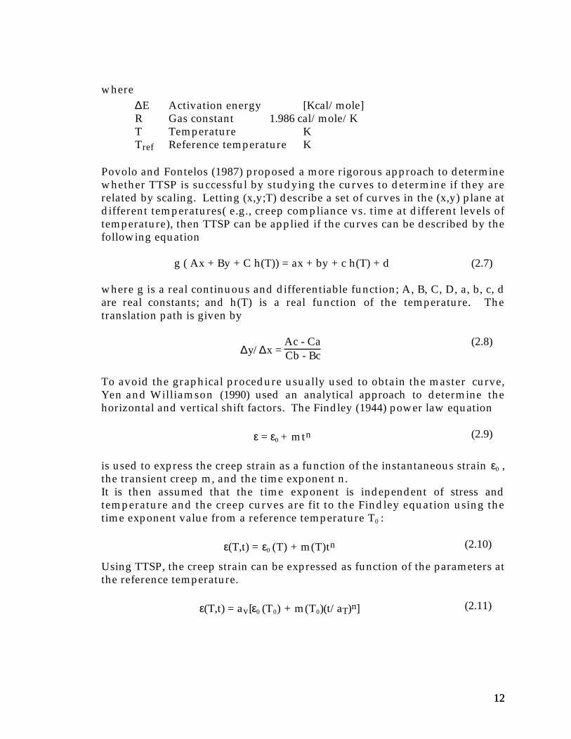
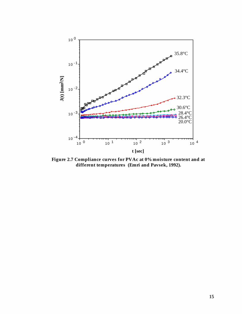
humidities above 65%. This creep acceleration due to increased moisturecontent leads to the possibility of applying a time-moisture equivalencescheme similar to time-temperature superposition where the temperaturewould be kept constant and the moisture content changed. Studies have beenconducted to assess the applicability of the principle of time-moisturesuperposition to some polymers. Emri and Pavsek (1992) conducted time-temperature and time-moisture superposition experiments on polyvinylacetate (PVAc) of medium molecular weight and a glass transitiontemperature of 30°C. The master curves at 20°C and zero moisture contentwere nearly identical. For the time-temperature experiment, samples weretested in torsion at zero moisture content at temperatures of 20, 26.4, 28.4, 30.6,32.3, 34.4, and 35.8°C. Figure 2.7 shows the shear compliance curves andfigure 2.8 shows the corresponding master curve. Similarly, torsion testswere conducted at 20°C and at moisture contents of 0, 0.74, 1.05, 1.29, 1.81, and2.72%. The compliance curves are shown on figure 2.9 and the master curveon figure 2.10. Superimposing the two master curves shows that they arenearly identical; this leads the authors to conclude that the principle of time-moisture superposition can be applied to PVAc under the conditionsconsidered in their experiments.In an earlier study to check the applicability of the principle of time-moisturesuperposition to crystalline polymers, Onogi et al. (1962) conducted stressrelaxation tests on polyvinyl alcohol (PVA) and nylon 6 films at varioustemperatures and moisture contents. For the PVA film with crystallinity of36.0 and 47.3%, time-temperature superposition could not be applied, evenwith vertical shifts. Figure 2.11 shows the relaxation modulus curves at 0%relative humidity and temperatures of 20, 40 , 60, 80, and 100°C. However, itwas possible to superpose the relaxation modulus curves at 20°C and relativehumidities of 0, 33, 45, 60, 65, and 75%, although the curves at the low andhigh humidities did not superpose very well. Figure 2.12 shows therelaxation curves and figure 2.13 shows the master curve. For nylon 6 film, stress relaxation tests were conducted at 0% relativehumidity and at temperatures ranging between 25 and 77°C. The curves attemperatures higher than 50°C superposed well while the curves attemperatures less than 50°C could not be superposed.

1515

10 410 310 210 110 010 -4

10 -3

10 -2

10 -1

10 0

t [sec]

35.8°C

34.4°C

32.3°C

30.6°C28.4°C26.4°C20.0°C

J(t)

[m

m2 /

N]

Figure 2.7 Compliance curves for PVAc at 0% moisture content and atdifferent temperatures (Emri and Pavsek, 1992).

1616

10 1010 810 610 410 210 010 -4

10 -3

10 -2

10 -1

10 0

t/aT [sec]

J(t)

[m

m2 /

N]

Tref = 20°C

Figure 2.8 Master curve from TTSP for PVAc at 0% moisture content (Emriand Pavsek, 1992).

1717

10 410 310 210 110 010 -4

10 -3

10 -2

10 -1

10 0

t [sec]

J(t)

[m

m2 /

N]

00.741.05

1.29

1.81

2.72

Figure 2.9 Compliance curves for PVAc at 20°C and at different moisturecontents (Emri and Pavsek, 1992).

1818

10 1010 810 610 410 210 010 -4

10 -3

10 -2

10 -1

J(t)

[m

m2 /

N]

t/aT [sec]

MCref = 0%

Figure 2.10 Master curve from TMSP for PVAc at 20°C (Emri and Pavsek,1992).

543210-110 8

10 9

10 10

Log t [sec]

E(t

) [d

ynes

/cm

2 ] 20°C40°C60°C80°C

100°C

Figure 2.11 Relaxation modulus curves at different temperatures for PVA(Onogi et al, 1962).

1919

54321010 9

10 10

10 11

Log t [sec]

E(t

) [d

ynes

/cm

2 ]

0% RH

33% RH

60% RH

65% RH75% RH

45% RH

Figure 2.12 Relaxation modulus curves at different relative humidities forPVA (Onogi et al, 1962).

Log t [sec]

E(t

) [d

ynes

/cm

2 ]

876543210-1-2-3-4-5-6-7-8-910 9

10 10

10 11

RHref = 65%

Figure 2.13 Master curve from TMSP at 20°C for PVA (Onogi et al, 1962).

For the time-moisture superposition tests, the samples were tested at 25°Cand at relative humidities of 0, 6, 19, 33, 43, 52, 64, 76, and 86%. The curvessuperposed well except at lower humidities. The authors conclude that it ispossible to apply the principle of time-moisture superposition provided thematerial is in the transition region.

2020

2.5 Application of TTSP to wood

One of the key assumptions behind the principle of time-temperaturesuperposition is that the material does not undergo any chemical or physicalchanges as a result of the temperature change (Ferry 1980). For wood twopossible changes may occur: the first one is a moisture content change, andthe second one is a change in the crystallinity of the cellulose. Bymaintaining the appropriate relative humidity in the testing chamber, it ispossible to maintain a constant moisture content under a constanttemperature. Also, Van der Put (1989) suggests that change in cellulosecrystallinity is very small within a reasonable temperature range.

The previous criteria do not guarantee the quantitative accuracy of theresults. Plazek (1965) suggests that the method is only valid in a limitedregion of time and temperature. When attempting to apply the principle oftime-temperature superposition to wood, we are faced with three mainobstacles:

(1) Under normal operating conditions, wood behaves in a glassy manner. Inthe glassy region, time effects are very small; this leads to large vertical shiftswhich do not conform to a pre-determined relation unlike the transition

region where the T0ρ

0/Tρ correction factor is used (Ferry, 1980). In a study onglassy poly(methyl methaccrylate), McCrum and Morris (1964) found that theshift factor follows an Arrhenius relation with a small activation energy (17Kcal). (2) Wood is highly crystalline; the cellulose in wood is about 70% crystalline.In a study on high density polyethylene, Nakayasu et al. (1961) report thatsimple superposition by horizontal shifting was ineffective; applying thetemperature correction factor did not help. The authors concluded that it waspossible to superpose the curves by applying two sets of shift factorscorresponding to two different mechanisms.

(3) Wood is a polymer blend with multiple transition zones: wood consistsof cellulose, lignin, and hemicellulose. These components depend differentlyon temperature. Fesko and Tschoegl (1971, 1974) studied the application oftime-temperature superposition to thermorheologically complex polymers,such as styrene/butadine/styrene block copolymers, and suggested a methodof superposition which accounts for the different temperature dependenciesof the components.

Although these wood properties limit the applicability of TTSP to wood, theydo not render the method invalid for wood. Many attempts have been madeto study the effect of temperature on wood; however, few attempts were made

2121

to apply the principle of time-temperature superposition to wood.Davidson(1962) conducted creep recovery experiments in bending andconcluded that time-temperature superposition should be used with cautionbecause wood is thermorheologically complex. However, Salmèn (1984) wassuccessful when he applied the principle to saturated wood samples attemperatures ranging from 20 to 140°C. In a study to determine the transitiontemperatures of the amorphous components in wood, Kelly et al. (1987) wereable to apply the principle of time-temperature superposition to woodsaturated with non-aqueous diluents. Gamalath (1991) superposedcompliance curves obtained from creep tests in compression for southernpine samples at temperatures between 20 and 60°C. Along with horizontalshifting, vertical shifts were needed to obtain a smooth master curve; thehorizontal shift factors followed an Arrhenius relation with an activationenergy of 30Kcal/mole.

Recently, a group of French researchers published the results of a study ontime-temperature superposition application to wood (Le Govic et al. 1987,1989). Creep tests in bending were conducted and the principle of time-temperature superposition was applied to obtain a compliance master curve.The curve was then fitted to a power law model. Seventy two French spruce(picea exeisa ) samples were tested in bending at temperatures of 25, 55, 65 and75°C, at a 12% moisture content, and load levels of 40, 30, 20 and 10% of theaverage short term ultimate loads. The horizontal shift factors followed anArrhenius relation with an activation energy of 162 kJ/mole (38.7Kcal/mole).Although the study produced a compliance master curve for over 60 years,compliance and master curves were not smooth and there is no mention ofpossible vertical shifts.

In order to successfully apply the principle of time-temperature superpositionto wood, a good understanding of the procedures used for synthetic polymerswith properties similar to wood is necessary. The following two sectionsreview the application of TTSP to crystalline and thermorheologicallycomplex materials.

2.6 Application of TTSP to thermorheologically complex materials

When a material is thermorhelogically complex, the horizontal shift factordepends on time in addition to temperature. This is illustrated in figure 2.14where the compliance curves at T1 and Tr, where Tr < T1, cannot besuperposed using a single shift factor. This is similar to superposingcompliance curves for thermorheologically simple materials as a function of

2222

temperature at various times (figure 2.15). If the shift factors follow the WLFrelation then the temperature shift factor is given by

∆T =C2 log(t / tr )

C1 − log(t / tr )(2.13)

Fesko and Tschoegl (1971) derived equations (2.13, 2.14) for determining theshift factors as a function of time; however, these equations cannot beintegrated which lead the authors to use a technique developed by Takayanagi(1965) which requires knowledge of the mechanical properties of thecomponents and their temperature functions:

∂ log D(t)

∂ log t

=

∂ log D t / aT( t)[ ]∂ logt / aT (t)

T r

1 −∂ log aT(t )

∂ log t

T

(2.14)

log aT (t)T

= −

D(T )T

t

∂D t / aT (t)[ ]∂ logt / aT (t)

Tr

−1 (2.15)

2323

log

D(t

)

log (t)

t1 t2t /a (T )T1 1

T

Tr

T 1log a (t )

t /a (T )T2 2

T 2log a (t )

Figure 2.14 Superposition on the time axis for thermorheologically complexmaterials.

2424

1T + ∆T1T

log

D(t

)

T

t t r

∆T

Figure 2.15 Superposition along the temperature axis.

Wood is a complex bio-composite material with many properties that makethe application of time-temperature superposition a challenge. However,similar studies on various thermorheologically complex polymers have beensuccessfully conducted. Obtaining a master curve is not a guarantee of thevalidity of TTSP. Long-term tests will be needed to assess the validity of themethod.

2.7 Creep Models

Gressel (1984) classified commonly used creep equations into mechanical,empirical, temperature, and molecular models. Empirical models are themost commonly used because of their simplicity; in particular the power lawmodel

(t) =1

E1+ atb( ) (2.16)

first applied to wood by Clouser (1959) , is frequently used.Because the constant a has units of t-b, equation 2.13 can be modified to yield

2525

(t) =1

E1 + A

t

b

(2.17)

(t) =1

E1 +

t

b

(2.18)

where = A− 1

b

A and b are dimensionless constants while τ and ρ have the dimensions of

time. The variable τ is the doubling time or the time required to reach twicethe instantaneous deformation. The power law function has the followingimplications (Nielsen 1984): Creep develops very rapidly at the beginningthen the rate approaches zero at long times

Nielsen (1984) suggests that the time exponent in the power law model isindependent of the environmental conditions. However the retardationtime depends on the temperature and humidity conditions as well as theangle between the load and the grain directions. A range for the timeexponent is given by Nielsen (1984):

Parallel to grain: 1/5 to 1/4Perpendicular to grain: 1/4 to 1/3

Le Govic et al. (1987) suggest the following model:

D(t,T ) = D0 1 +t

0

k

exp−kW

RT

(2.19)

Where D0 is the instantaneous compliance, W is the activation energy from

the Arrhenius relation, and τ0 is the retardation time at infinite temperature.The parameters from LeGovic's study are:

D0 = 0.5866 x 10-4 MPa-1 = 4.0455x10-7 in2/lbW = 162.66 kJ/mole = 38.7 Kcal/molek = 0.112τ0 = 1.22x10-16 s

The activation energy of 38.7 kJ/mole is comparable to the one found byGamalath (1991). Le Govic (1989) suggests that although the power law modelis widely used, an exponential law would be more suitable for building codes.

2626

Such exponential laws were proposed for the EUROCODE 5. Specifically, forbending

t − t0( ) =E

1+ 0.65 1 + 0.65 1 − e−( t − t0 )( )( )[ ] (2.20)

and for compression

t − t0( ) =E

1+ 0.30 1 + 0.30 1 − e−( t −t 0 )( )( )[ ] (2.21)

Huet and Navi (1990) proposed a model which accounts for themultitransitional nature of wood. This model consists of a series of modifiedKelvin elements where the dashpots are replaced by a power law creep model.Each element has unique parameters that correspond to each transition.

2.8 Finite Element Analysis for Creep

The finite element method is a powerful and well established tool for stressanalysis. Therefore, when researchers became interested in solving creepproblems numerically, they turned to the finite element method rather thanfinite difference and direct integration methods (Kraus, 1980). The subject offinite element analysis has been addressed by many authors such asZienkiewicz (1971) and Bathe (1982).

2.8.1 Creep Models

In statically indeterminate structures, such as space frames and lattice domes,the creep differences within the structure cause extensive long-term stressredistributions, even under constant loads. Therefore, creep laws must beformulated for variable stresses. Moreover, any creep analysis must proceedin an incremental manner with suitable time steps, and iteration within timesteps is frequently required to satisfy the creep law and assure convergence(Bathe, 1982). In the one-dimensional case, the creep strain can be expressedas a function of the stress, temperature, and time:

c = f ( ,T,t) (2.22)

It is usually assumed that these effects are independent, then the creep straincan be expressed as (Kraus, 1980)

2727

c = f i(T )i =1

n

∑ gi( ) hi(t)(2.23)

This allows for more than one term in the expression. In order to account forthe change in stress or temperature, two options are available. The first is theequation of state, or rate-type, formulation where the creep strain depends onthe present state and the second is the hereditary, or integral-type,formulation where the response depends on the entire loading history.Although the hereditary model would yield better results (Kraus, 1980), it isnot commonly used because it requires extensive storage and more elaboratematerial testing. The equation of state approach is widely used because it iseasy to incorporate into available computer programs. Procedures have beendeveloped to convert the hereditary integral into a state equation (Chan 1983;Kabir 1976; Nilson 1982). This has been accomplished, for example, byexpanding the compliance function in a Dirichlet series (Kabir 1976):

D ,t − ,T( ) = aii =1

m

∑ ( ) 1 − e− i T( ) t −( )[ ] (2.24)

where ai( ) is a scale factor depending on the time of loading τ, i areexponential constants, and T( ) is the temperature shift function.In order to use the equation of state formulation, the Bailey-Norton law iscommonly used:

c = A mtn (2.25)

where A, m, and n depend on temperature; also m is greater than one and nis a fraction. The rate of creep strain is obtained by differentiating the aboveequation with respect to time; this is referred to as the time-hardeningformulation of the equation of state:

˙ c = A mnt n−1 (2.26)

Solving Eq. 2.25 for time, we obtain

t =c

A m

1n

(2.26

which when introduced into the time hardening equation produces thestrain-hardening formulation of the equation of state:

2828

˙ c = A mnc

A m

n −1n

= A1

n

m

n n cn−1

n

(2.27)

Although the time and strain hardening formulations are derived from thesame equation, they yield different results when the applied stress is notconstant, as illustrated in Figure 2.16. For time hardening, when the stress

changes from σ3 to σ4, the strain is resumed on the σ4 curve at the time ofchange whereas for strain hardening, the strain resumed where it stopped on

the σ3 curve. Kraus (1980) states that based on experimental results, the strainhardening formulation gives better results; this is also noted by Bushnell(1977).

2929

σ1

σ2

σ3

σ4

time

cree

p st

rain

strain hardening

time hardening

stre

ss

time

σ1

σ2

σ4

σ3

Figure 2.16 Time and strain hardening responses to variable stress.

3030

2.8.2 Computer Programs

With few exceptions, finite element computer programs for the analysis ofcreep problems are based on the initial strain method (Boyle and Spence 1983;Bushnell 1977; Kraus 1980; Nickell 1974). The initial strain method wasmotivated by the similarity of creep problems to thermal stress problems(Greenbaum and Rubinstein 1968; Mendelson et al. 1959; Zienkiewicz andWatson 1966), where the method was first proposed. A shortcoming of early applications, the requirement of small time steps toachieve convergence (Nickell 1974), has been overcome by thesubincrementation of time steps and effective time integration algorithms(Bushnell 1977; Snyder and Bathe 1981; Zienkiewicz and Cormeau 1974). Inaddition, the initial strain method can be used to investigate the effect ofstructural imperfections (e.g., lack-of-fit problems caused by fabrication errors)or flaws in connections. This will be useful in large assemblies of elementssuch as lattice domes. Moreover, it permits one to represent the effect ofcreep in connections as a structural imperfection.For this study, ABAQUS, a commercial finite element program was used. Ithas powerful nonlinear analysis capabilities that allow for automatic timeintegration and iteration. For linear elastic materials, creep properties can beassigned either by supplying the constants for the Bailey-Norton law or byusing a special subroutine that computes the creep strain increment at eachiteration. The last method allows for introduction of temperature andmoisture effects.

2.8.3 Creep Stability

According to Britvec (1973), a body is stable if it tends to regain its originalstate after being disturbed by an external effect. To determine if a column isstable, an infinitessimal velocity is applied at time t=0. The column is stable ifthe motion decreases with time and is unstable otherwise. For elasticmembers and systems, the problem consists of finding the critical load forwhich the system becomes unstable. For viscoelastic materials, however, theproblem becomes more complicated as the critical load depends on time andon the magnitude of the applied impulse for nonlinear creep. The finiteelement method can be used to determine the time to failure by checking thetangent stiffness matrix along the equilibrium path. The system is stable ifthe stiffness matrix is positive definite and unstable otherwise.

3131

2.8.4 Creep Analyses

The finite element method will be used to study the effect of long-term creepon columns, arches, and lattice domes. Of primary interest is the extent towhich creep can reduce the load-carrying capacity. The possibility of creepbuckling of arches and lattice domes will be investigated.

3232

3. EXPERIMENTAL

The purpose of the experimental study is: (1) to use the principle of time-temperature superposition to develop a power law model for long-termcreep, and (2) to compare the resulting master curve to long-term creepcurves. The power law model will then be used to conduct finite elementanalyses on simple and complex wood structures.

3.1 Dynamic tests using the DMA

A TA Instruments DMA (Dynamic Mechanical Analyzer) was used to detecttransitions and to conduct creep tests at temperatures between 25 and 80°C.The DMA has the advantage of quickly giving results, however, it does notallow for control of the moisture content of the sample. The DMA was usedin two modes: fixed frequency and creep.Fixed frequency. In fixed frequency tests, the sample is bent at apredetermined frequency and the storage compliance, loss modulus, and losstangent are recorded as the temperature is increased at a specified rate. Afrequency of 1 Hz and a temperature rate of 2°C/minute were used.Creep. Creep experiments on the DMA are simple to perform. The sample ismounted in the grips and the grips are tightened using screws. The constantstress is prescribed by assigning an initial displacement ( 0.1 - 0.3 mm ). Thesample creeps for 15 minutes then recovers for 45 minutes. The temperatureis then increased by a predetermined amount and the process is repeated untila maximum temperature is reached. The data is read and manipulated by theon-line computer system and the results can be displayed as the experimentprogresses.

3.2 Short-term creep tests

Short-term creep tests in tension and in compression were conducted toobtain creep compliance curves at different temperatures while maintaining aconstant moisture content. The following test parameters were used.

Specimens. Southern yellow pine, Douglas-fir, yellow-poplar, Parallam™were tested. These species were chosen to reflect the current trends in woodusage. Southern yellow pine and Douglas-fir are used extensively as lumberand as materials for several wood composites such as glulam. Yellow-poplaris used in Parallam, laminated veneer lumber and other products.Parallam™ is a structural composite lumber product gaining popularitybecause of its availability in large sizes.

3333

Size. Specimen dimensions are a compromise between the load magnitudethat can be applied and the size that would be representative of the species. For tension the size chosen is 0.25 x 0.5 x 12 in. The size for the compressiontest is 0.75 x 0.75 x 4 in.Number of specimens. The number of specimens is subject to two conflictingrestrictions. On one hand, wood is a variable material which requires testingmany specimens for statistical accuracy, on the other hand, the time availablefor the tests is limited and so is the availability of the equipment. For thisstudy, 12 samples of each species were tested.

Load. Wood is considered to behave in a linear viscoelastic manner for loadsbelow 50% of the ultimate load (Schniewind 1968, Nielsen 1984). Schaffer(1983) describes the behavior of wood as nonlinear regardless of the loadlevel; however, he states that at low stresses, linear behavior can be a goodapproximation of the behavior and Boltzmann's superposition principleapplies for stresses up to 40% of the short-term strength. Le Govic (1988) giveslimits for linear behavior of 30-35% of the short-term strength for bendingand up to 50% of the short-term strength for tension. To insure that behaviorof test specimens remains within the linear range, loads in the 20 to 25%range of the short-term ultimate strength were.

Testing apparatus. Creep experiments are very sensitive because thedeformations are very small. Because each sample is loaded and unloadedseveral times, any perturbation to the sample can adversely affect the results. Each sample is mounted to grips and the load is applied and removed using ahydraulic jack (Figure 3.1). Figure 3.2 shows the tension and compressionspecimen holders which were designed and built for this project.

3434

Insulated Chamber

Loading Frame

Grip

Sample

Weight

SupportingFrame

HydraulicJack

Figure 3.1 Tension test apparatus

3535

sample

(a) (b)

Figure 3.2 Creep apparatus (a) tension, (b) compression.

Environmental conditions. The testing apparatus is housed in an insulatedchamber, conditioned air is circulated through the chamber to maintain aconstant 12% moisture content. The temperatures used are 20, 30, 40, 50, 60 ,70, and 80°C. The relative humidity required to maintain a 12% moisturecontent can be calculated using the Hailwood-Horobin model (Simpson 1971).Table 3.1 shows the corresponding values of temperature and relativehumidity to maintain 6, 9, and 12% moisture contents. The primary targetEMC for the test specimens in this study will be 9% MC to reflect the averageEMC for most of the country. Additionally, specimens were tested at 6 and12% EMC for three reasons: (1) There is a historic precedence for reporting

3636

wood properties at a standard 12% MC since this is an easy condition toachieve and the results will be readily comparable with the results of others;(2) 12% MC represents the upper range EMC of normal interior exposure forwood products and the average for protected exterior exposure (Oviatt, 1968);(3) the additional EMC levels will enhance our understanding of theapplication and suitability of the time-temperature superposition principle towood.

Table 3.1 Relative humidity required to maintain a 12% moisture content.

Temperature

°C

Temperature(Dry bulb)

°F

RelativeHumidity

for 6 % MC

RelativeHumidity

for 9 % MC

RelativeHumidity

for 12 % MC

20.0 68.0 29.2 48.7 64.525.0 77.0 29.8 49.6 65.430.0 86.0 30.7 50.8 66.535.0 95.0 31.8 52.2 67.740.0 104.0 33.1 53.7 69.045.0 113.0 34.6 55.4 70.450.0 122.0 36.2 57.2 71.855.0 131.0 38.0 59.0 73.360.0 140.0 40.0 60.9 74.965.0 149.0 42.0 62.9 76.470.0 158.0 44.2 64.8 77.975.0 167.0 46.4 66.7 79.480.0 176.0 48.7 68.7 80.9

Test duration. Figure 3.3 shows the log time axis for times ranging from 1second to 50 years. Depending on the horizontal shift factors, a creep periodof as little as 4 hours can be sufficient to extrapolate to 50 hours. A creepduration of six to twelve hours is chosen. Another consideration for theduration of the creep test is that the load is not applied instantly, but over aperiod of time (ramp load). Nielsen (1984) suggests a test duration of 1-10 days

3737

to account for ramp loading. A recovery period of three times the creepperiod is used to recover most of the creep deformation. In her study,Gamalath (1991) used a creep period of 17 hours and a recovery period of 40hours.

4 h

ou

rs

1ho

ur

1wee

k

1 y

ear

10 y

ears

20 y

ears

30 y

ears

40 y

ears

50 y

ears

10987654321024

ho

urs

Figure 3.3 Log time axis (seconds)

Mechanical Conditioning. The wood specimens used in the creepexperiments were not subjected to significant loads prior to the tests. Thespecimens need to be mechanically conditioned to obtain consistent results.In his creep recovery experiments, Davidson (1962) used a mechanicalconditioning program that consisted of six 10-hour creep tests at 60°Cfollowed by a recovery period of two weeks. The specimens were alsoconditioned at every temperature decrement for two days. In this study, thespecimens were subjected to repeated cycles of creep and recovery until thecompliance curves were reasonably close. To determine the effect ofmechanical conditioning, three southern pine samples were tested in tensionat 25°C for 4 hours of creep and 20 hours of relaxation, the results are shownin figures 3.4, 3.5, and 3.6. It can be concluded that one or two cycles areenough to get close results.

3838

5.54.53.52.51.50.5-6.30

-6.28

-6.26

-6.24

-6.22

LOG time [sec]

LO

G C

om

pli

ance

[in

^2/

lb]

first test

third test

fourth test

fifth test

Figure 3.4 Mechanical conditioning of sample 1 at 25°C.

3939

5.54.53.52.51.50.5-6.34

-6.33

-6.32

-6.31

-6.30

-6.29

-6.28

LOG time [sec]

LO

G C

om

pli

ance

fourth test

fifth test

Figure 3.5 Mechanical conditioning of sample 2 at 25°C.

4040

5.54.53.52.51.50.5-6.30

-6.29

-6.28

-6.27

-6.26

-6.25

-6.24

LOG time [sec]

LO

G C

om

pli

ance

[in

^2/

lb]

first test

third test

fourth test

fifth test

Figure 3.6 Mechanical conditioning of sample 3 at 25°C

Strain measurement and data acquisition. The strain is measured using 350strain gages connected in a Wheatstone bridge as shown in figure 3.7. Twostrain gages are mounted on the specimen and the other two on a dummyspecimen to account for self heating of the strain gages due to the poorthermal conductivity of wood. The bridge output voltage is measured andconverted to strain using an Hewlett Packard data acquisition system.

4141

R1

R2

R4

dummy specimen

lead wires

R3

active specimen

(a)

E 0E1

R1 R2

R3R4

(b)

Figure 3.7 (a) active and dummy specimens; (b) Wheatstone bridge.

3.3 Long-term creep tests

Long-term creep tests in tension and in bending were conducted to serve as abasis for comparison with the results from short-term creep tests. The testswere conducted in an air-conditioned room with an equilibrium moisturecontent of 12%. Three species were tested in tension and in compression. 3.2 shows the number of samples for each species while figure 3.8 and 3.9show the sample arrangement.

Table 3.2 Number of samples in the long-term creep test.

4242

Species number of samples incompression

number of samples intension

Yellow-poplar 4 3Douglas-fir 4 0Southern yellow pine 4 4

4343

R9

yellowP

oplarT

ension

R7

yellowpoplarT

ension

R5

southernpineT

ension

R4

southernpineT

ension

R3

southernpineT

ension

R2

yellowP

oplarC

ompression

R1

yellowpoplarC

ompression

R8

yellowpoplarT

ension

R6

southernpineT

ension

Weight

L1yellow P

oplarC

ompression

L2southern pineC

ompression

L3southern pineC

ompression

L4southern pineC

ompression

L5southern pineC

ompression

L6yellow P

oplarC

ompression

R10

Load cell

L7Douglas fir

Com

pression

L8Douglas fir

Com

pression

L9Douglas fir

Com

pression

L10D

ouglas Fir

Com

pression

NotConnected

Weight

Figure 3.8 Sample arrangement for the long-term creep tests.

4444

The sample holders for tension and compression were the same as the onesused in the short-term experiments. The strain was read using two strainindicators and two switch and balance units, readings were taken at increasingtime intervals. A load cell was used to monitor the load to insure that therewas no reduction in load due to friction at the pulleys.

Figure 3.9 Long-term creep test setup.

4545

4. RESULTS

4.1 Dynamic tests

4.1.1 Fixed frequency tests

It was observed in preliminary experiments that the wood samples wouldlose most of their moisture during the test, this lead to incorrect results sincethe wood behavior depends greatly on moisture content. To quantify theamount of moisture loss, some samples were weighed before and after thetest, then dried and weighed again to measure the moisture contents beforeand after the test. Typical results are shown in Table 4.1.

Table 4.1 Moisture loss during fixed frequency test (25 to 80°C at 2°C /minute).

Species Starting moisture content(%)

ending moisture content (%)

southern pine 13.0 4.8Douglas-fir 11.4 4.3

This reduction in moisture will not allow for the accurate detection oftransitions. To reduce moisture loss, the samples were painted withaluminum paint which is a good moisture barrier. Although some moisturewas lost it was very small relative to the unpainted samples; typical resultsare shown in Table 4.2.

Table 4.2 Moisture loss during fixed frequency test for painted samples (25 to80°C at 2°C / minute).

Species Starting moisture content(%)

ending moisture content(%)

Southern pine 13.0 12.5Douglas-fir 11.4 10.8

The effect of painting the samples on the fixed frequency test results can beseen for southern pine and Douglas-fir samples in figures 4.1 and 4.2 Thesouthern pine and Douglas-fir samples had starting moisture contents 13.0 ofand 11.4%, respectively.

4646

0.03

0.04

0.05

0.06

0.07ta

n δ

20 30 40 50 60 70 80 90

Temperature (°C)

unpainted sample, 1 Hz

unpainted sample, 0.3 Hz

painted sample, 1 Hz

painted sample, 0.3 Hz

Figure 4.1 Loss tangent for painted and unpainted southern pine samples.

4747

0.02

0.03

0.04

0.05

0.06

0.07

0.08

0.09

tan

δ

20 30 40 50 60 70 80 90

Temperature (°C)

unpainted sample, 1 Hz

unpainted sample, 0.3 Hz

painted sample, 1 Hz

painted sample, 0.3 Hz

Figure 4.2 Loss tangent for painted and unpainted Douglas-fir samples.

Moisture loss from the samples results in higher transition temperatures; forsouthern pine the difference is at least 20°C. It should be noted however thatthe loss tangent for the painted samples is about half that of the paintedsamples, this may indicate that the paint is influencing the response.Once the moisture loss problem was resolved several tests were conducted todetermine any transitions in samples of southern pine, Douglas-fir, andyellow-poplar at different moisture contents. Once the samples reached thedesired equilibrium moisture content, they were painted and tested soon afterthe paint was dry. The results at frequencies of 1 Hz at 5, 7, and 9% moisturecontent are shown in figure 4.3 for yellow-poplar. At 5% m.c. there is a

4848

transition at 70°C. At 7% m.c. the transition is at 60°C, whereas at 9% m.c.there is a transition at 65°C.

0.04

0.045

0.05

0.055

0.06

0.065

0.07

0.075T

an δ

20 30 40 50 60 70 80 90

Temperature (°C)

9% moisture content

7% moisture content

5% moisture content

Figure 4.3 Loss tangent for yellow-poplar at 5, 7, and 9% moisture contents.

For southern pine (figure 4.4) and Douglas-fir (figure 4.5), the transitionsbegin around 70°C and extend beyond the maximum test temperature.

4949

0.05

0.055

0.06

0.065

0.07

tan

δ

20 30 40 50 60 70 80 90

Temperature (°C)

9% m.c.

13.0% m.c.

Figure 4.4 Loss tangent for southern pine at 13.0 and 9% moisture contents.

5050

0.05

0.06

0.07

0.08

0.09

tan

δ

20 30 40 50 60 70 80 90

Temperature (°C)

9.5% m.c.

12.5% m.c.

Figure 4.5 Loss tangent for Douglas-fir at 12.5 and 9.5% moisture contents.

The results obtained are consistent with those of Kelly et al. (1987): Foryellow-poplar, the transition at 5 and 7% m.c. correspond to lignin whereasthe transition at 9% m.c. is attributed to hemicellulose. At 12 and 9% m.c. thetransitions in southern pine and Douglas-fir are attributed to hemicellulose.This is a cause of concern for two reasons: (1) wood is clearlythermorheologically complex with two transitions; (2) the transitions areclose to the short-term test temperature and moisture content ranges.

5151

4.1.2 Creep Tests

The advantages of using the DMA for creep tests are speed, unattendedoperation, automatic data collection and reliability. The following parametersrecommended by a colleague (Chang, 1991) who used the DMA extensivelywere used:

15 min creep, 45 min recoveryTime to equilibrate the temperature: 1 minTemperature increments: 10°CSpan: varied between 25 and 40 mm

At first, tests were conducted on unpainted samples which quickly lostmoisture. Consequently, the creep curves could not be superposed beyondthe second temperature increment. Then some samples were painted withaluminum paint and tested. Due to the long duration of the tests, moisturestill escaped and the creep curves could not be superposed. Two examples areshown in figures 4.6 and 4.7 for yellow-poplar at 5 and 7% moisture content,respectively.

Log

Com

plia

nce

(1/P

a)

Log time (sec)

75°C

65°C

55°C

45°C

35°C

25°C

-9.9

-9.8

-9.7

-9.6

-9.5

-9.4

-1 -0.5 0 0.5 1 1.5 2 2.5

Figure 4.6 Compliance curves for yellow-poplar at 5% moisture content.

5252

Log time (sec)

-9.8

-9.75

-9.7

-9.65

-9.6

-9.55

Log

com

plia

nce

(1/P

a)

-1 -0.5 0 0.5 1 1.5 2 2.5

75°C

65°C

55°C

45°C

35°C

25°C

Figure 4.7 Compliance curves for yellow-poplar at 7% moisture content.

The DMA is a useful tool for detecting transitions in polymers and forconducting creep tests for TTSP. However, the lack of humidity controlmakes it inadequate for wood. The fixed frequency tests revealed that thewood is undergoing a transition between 60 and 80°C at moisture contentsbetween 5% and 10%. Superposition of the creep test curves was not possiblebeyond 40°C for most tests; although the loss of moisture is a major factor, thepresence of transitions can also be a factor.

4.2 Short-Term Creep Tests

The short-term creep tests were the most challenging part of the research.Several problems were encountered and attempts to correct them were made.This led to overall improvements of the results. Short-term creep resultswere discussed by Tissaoui et al. (1992) and Bond (1993).

4.2.1 Difficulties

The main problems were maintaining a constant temperature and relativehumidity, maintaining a constant moisture content from one test to the next,

5353

applying the load in a consistent manner, and the possible creep of the straingage adhesive.EnvironmentIt was noticed that the data was not smooth, especially at the highertemperatures. Variations in the temperature and relative humidity weresuspected. To check this hypothesis, the temperature and relative humiditywere monitored during each test and it was found that the temperature andrelative humidity were fluctuating; this led to a change in the moisturecontent of the samples during the test. To maintain a constant temperatureand relative humidity, a new environmental chamber with thickerinsulation and a better access door was built. Aluminum paint was appliedfor added protection especially at the higher temperatures. The result was amarked reduction in temperature and relative humidity fluctuation althoughslight variation still occurred at the highest temperatures of 70 and 80°C,especially when the target moisture content was 12%.Moisture contentIn order to apply TTSP, it is necessary to maintain a constant moisturecontent when increasing the temperature between tests. Three dummysamples were placed in the testing chamber to determine the moisturecontent. The Hailwood-Horobin model (Simpson 1971) was used toapproximate the required relative humidity to maintain the desired moisturecontent. However, adjustments had to be made until the moisture contentwas stable. This process took from two to four days which added to the timerequired to complete the tests.Load applicationIt is important to apply the load consistently from one test to the next. Insome of the tests, the weight rotated or was applied faster than in others. This led to inconsistent results especially for tests that last for short periods oftime (hours); problems included fluctuation of the data and variation in theinitial compliance. Great efforts were made to insure that the load wasreleased at the same rate with minimum disturbance.Strain gagesUnless the strain gage adhesive (an epoxy) is cured at a higher temperaturethan the specimen will be subjected to, it can creep leading to errors in strainmeasurements (especially at the higher temperatures). To eliminate thisproblem, the samples were placed in an oven at 95°C for about 15 minutes. Itwas also suggested by the gage manufacturer that a pre-coat of adhesive beapplied prior to installing the strain gages. This however did not change theresults.

4.2.2 Creep in tension

Creep experiments in tension were conducted on southern yellow pine,Douglas-fir, and yellow-poplar samples. Figure 4.7 shows the compliance

5454

curves and the master curve obtained by superposition for a yellow-poplarsample at 6% moisture content. The extrapolated data from five hour testscorresponds to about 75 days. The horizontal shift factors follow anArrhenius relation since the relation between the temperature and thehorizontal shift factors is linear as shown in Figure 4.8; the correspondingactivation energy is 92.5 kJ/mole. The master curve was fitted to the power law equation using a nonlinearfitting procedure (SAS Innstitute INC., 1989). The resulting parameters were:

D0 = 6.0475 x10-11 Pa-1

b = 1.047 x10-3 sec-k

k =0.273

Figure 4.9 shows the master curve and the curve corresponding to the powerlaw equation.

25°C

35°C

45°C

55°C

65°C

LOG time [sec]

LO

G C

ompl

ianc

e [1

/Pa]

7.06.56.05.55.04.54.03.53.02.52.01.51.0-10.22

-10.21

-10.20

-10.19

-10.18

-10.17

-10.16

(a)

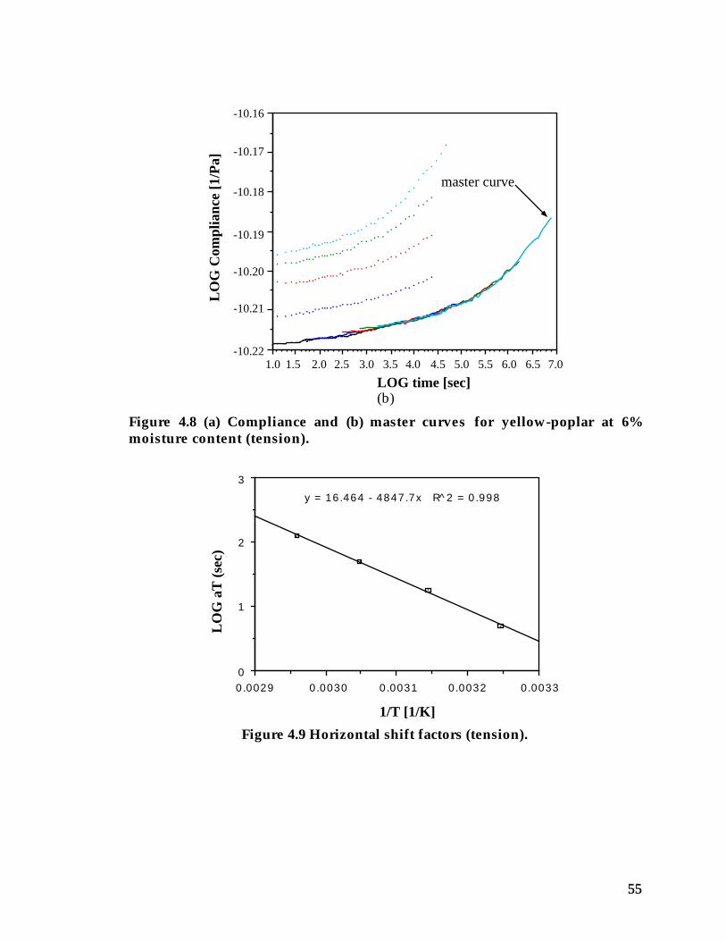
5555

7.06.56.05.55.04.54.03.53.02.52.01.51.0-10.22

-10.21

-10.20

-10.19

-10.18

-10.17

-10.16

LOG time [sec]

LO

G C

ompl

ianc

e [1

/Pa]

master curve

(b)

Figure 4.8 (a) Compliance and (b) master curves for yellow-poplar at 6%moisture content (tension).

0.00330.00320.00310.00300.00290

1

2

3

1/T [1/K]

LO

G a

T (

sec)

y = 16.464 - 4847.7x R^2 = 0.998

Figure 4.9 Horizontal shift factors (tension).

5656

86420-10.22

-10.21

-10.20

-10.19

-10.18

Master curve

Power law fit

LOG time [sec]

LO

G C

ompl

ianc

e [1

/Pa]

Figure 4.10 Master curve and power law fit (tension).

Creep test on southern pine, Douglas-fir, and yellow-poplar in tension at 6%m.c.

As shown in figure 4.11, the environmental conditions remain constantthroughout the creep tests. The creep could be superposed at all temperaturesexcept for the curves at 65°C for southern pine. The compliance and mastercurves are shown in figures 4.12, 4.14, and 4.16, and the shift factors areplotted in figures 4.13, 4.15, and 4.17. The activation energies were 74.6, 128.0,and 90.7 kJ/mole for southern pine, yellow-poplar and Douglas-fir,respectively. The master curves were fit to the power law equation and theparameters are shown in table 4.3.

5757

20

30

40

50

60

70

Tem

pera

ture

(°C

)

1 2 3 4 5

Log time (sec)

30

35

40

45

Rel

ativ

e hu

mid

ity (%

)

1 2 3 4 5

Log time (sec)

Figure 4.11 temperature and relative humidity during the test.

-10.34

-10.33

-10.32

-10.31

-10.3

-10.29

1 2 3 4 5 6 7 8

65°C curve was not shifted

Log time (sec)

65°C

55°C

45°C

35°C

25°C

Log

Com

plia

nce

(1/P

a)

Figure 4.12 Compliance and master curves for southern pine at 6% moisturecontent (tension).

5858

0.75

1

1.25

1.5

1.75

Log

aT (

sec)

0.003 0.00305 0.0031 0.00315 0.0032 0.00325

1/T (K)

y = -4060.800x + 14.145 r2 = 0.932

Figure 4.13 Horizontal shift factors for southern pine, DH=74.6 kJ/mole.

5959

-10.16

-10.15

-10.14

-10.13

-10.12

-10.11

1 2 3 4 5 6 7 8

Log time (sec)

65°C

55°C

45°C

35°C

25°C

Log

Com

plia

nce

(1/P

a)

Figure 4.14 Compliance and master curves for yellow-poplar at 6% moisturecontent (tension).

6060

0.5

1

1.5

2

2.5

3

Log

aT (

sec)

0.0029 0.003 0.0031 0.0032 0.0033

1/T (K)

y = -6685.081x + 22.622 r2 = 0.973

Figure 4.15 Horizontal shift factors for yellow-poplar, DH=128.0 kJ/mole.

6161

Log time (sec)

65°C

55°C

45°C

35°C

25°C

Log

Com

plia

nce

(1/P

a)

-10.22

-10.21

-10.2

-10.19

-10.18

-10.17

1 2 3 4 5 6 7 8

Figure 4.16 Compliance and master curves for first at 6% moisture content(tension).

6262

0.5

1

1.5

2

2.5

Log

aT (

sec)

0.0029 0.003 0.0031 0.0032 0.0033

1/T (K)

y = -4737.138x + 16.171 r2 = 0.999

Figure 4.17 Horizontal shift factors, DH=90.7 kJ/mole.

Table 4.3 Power law parameters for southern pine, yellow-poplar, andDouglas-fir at 6% moisture content in tension.

D0 (Pa-1) b (sec-k) kSouthern pine 4.503x10-11 0.0117 0.1256Douglas-fir 6.049x10-11 0.00135 0.2546yellow-poplar 6.918x10-11 0.00779 0.1497

4. 2 .3 Creep in compression

Creep in compression was conducted on southern yellow pine, Douglas-fir,and yellow-poplar samples. Figure 4.18 shows the compliance curves andmaster curve for a Douglas-fir sample at 9% moisture content. Thehorizontal shift factors (figure 4.19) follow an Arrhenius relation as indicatedby the linear relation between the shift factors and the temperature. Thecorresponding activation energy is 20.0 Kcal/mole.The compliance curves for the Douglas-fir sample at 20, 30, 50, and 60°C weresuperposed to obtain a master curve which was then fitted to the power lawequation; the parameters are:

6363

D0 = 8.374 x10-11 Pa-1

b = 2.53 x10-3 sec-k

k = 0.248

Figure 4.20 shows the master curve from the experimental data as well as thecurve from the power law equation. The master curve extrapolated the shortterm creep data to about 30 days from 4 six hour tests; compliance curves at 70and 80°C would provide more extrapolation of the data; however, unstableenvironmental conditions prevented the collection of the creep data.

6464

LOG time [sec]

LO

G C

ompl

ianc

e [1

/Pa]

7.06.56.05.55.04.54.03.53.02.52.01.51.0-10.08

-10.06

-10.04

-10.02

-10.00

20°C

30°C

40°C

50°C

60°C

(a)

7.06.56.05.55.04.54.03.53.02.52.01.51.0-10.08

-10.06

-10.04

-10.02

-10.00

LOG time [sec]

LO

G C

ompl

ianc

e [1

/Pa]

master curve

(b)

Figure 4.18 (a) Compliance and (b) master curves for Douglas-fir at 9%moisture content (compression).

6565

0.00340.00330.00320.00310.00300.5

1.0

1.5

2.0

2.5

1/T [1/K]

LO

G a

T [

sec]

y = 15.340 - 4377.3x R^2 = 0.968

Figure 4.19 Horizontal shift factors (compression).

Fitted data

Experimental data

LOG time [sec]

86420

-10.08

-10.07

-10.06

-10.05

-10.04

-10.03

LO

G C

ompl

ianc

e [1

/Pa]

Figure 4.20 Master curve and power law fit (compression).

6666

Creep test on southern pine, Douglas-fir, and Parallam™ in compression at6% m.c.

Figure 4.21 shows that the environmental conditions remain constantthroughout the creep tests. Except for the curves at 70 and 80°C, the curvescould be superposed to form a master curve The compliance and mastercurves are shown in figures 4.22, 4.24, and 4.26, and the shift factors areplotted in figures 4.23, 4.25, and 4.27. The activation energies were 108.7, 109,and 129 kJ/mole for southern pine, Douglas-fir, and Parallam™, respectively.The master curves were fit to the power law equation and the parameters areshown in table 4.4.

20

30

40

50

60

70

80

Tem

pera

ture

(°C

)

1 2 3 4 5

Log time (sec)

45

50

55

60

65

70

Rel

ativ

e Hum

idity

(%)

1 2 3 4 5

Log time (sec)

Figure 4.21 Temperature and relative humidity during the test.

6767

-10.34

-10.32

-10.3

-10.28

-10.26

-10.24

Log

Com

plia

nce (

1/Pa

)

Log time (sec)

80°C

70°C

60°C

50°C

40°C

30°C

20°C

70 and 80°C curves were not shifted.

1 2 3 4 5 6 7 8

Figure 4.22 Compliance and master curves for southern pine at 9% moisturecontent (compression).

6868

0.5

1

1.5

2

2.5

Log

aT (

sec)

0.003 0.0031 0.0032 0.0033 0.0034

1/T (K)

y = -5679.022x + 19.548 r2 = 0.982

Figure 4.23 Horizontal shift factors for southern pine at 9% moisture content,

H = 108.7 kJ/mole.

6969

-10.1

-10.05

-10

-9.95

-9.9

1 2 3 4 5 6 7 8

Log

Com

plia

nce

(1/P

a)

Log time (sec)

80°C

70°C

60°C

50°C

40°C

30°C

20°C

70 and 80°C curves were not shifted.

Figure 4.24 Compliance and master curves for Douglas-fir at 9% moisturecontent (compression).

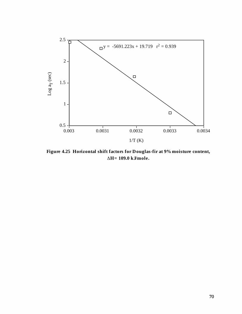
7070

0.5

1

1.5

2

2.5

Log

aT (

sec)

0.003 0.0031 0.0032 0.0033 0.0034

1/T (K)

y = -5691.223x + 19.719 r2 = 0.939

Figure 4.25 Horizontal shift factors for Douglas-fir at 9% moisture content,

H= 109.0 kJ/mole.

7171

Log

Com

plia

nce

(1/P

a)

Log time (sec)

80°C

70°C

60°C

50°C

40°C

30°C

20°C

-10.375

-10.35

-10.325

-10.3

-10.275

-10.25

1 2 3 4 5 6 7 8

70 and 80°C curves were not shifted.

Figure 4.26 Compliance and master curves for Parallam™ at 9% moisturecontent (compression).

7272

0.5

1

1.5

2

2.5

3

Log

aT (

sec)

0.003 0.0031 0.0032 0.0033 0.0034

1/T (K)

y = -6747.071x + 23.306 r2 = 0.965

Figure 4.27 Horizontal shift factors for Parallam™ at 9% moisture content,

H= 129.2 kJ/mole.

Table 4.4 Power law parameters for southern pine, Douglas-fir, andParallam™ at 6% moisture content.

D0 (Pa-1) b (sec-k) kSouthern pine 4.697x10-11 0.00411 0.2163Douglas-fir 8.815x10-11 0.00472 0.2083Parallam™ 4.418x10-11 0.00403 0.2006

Superposition of the compliance curves was possible at temperatures below60°C; however, it was not possible to superpose most of the curves at 70 and80°C. The activation energies obtained were within published results(Gamalath, 1991). Once the master curves were constructed, the power lawequation parameters were determined, the exponents were within the rangeproposed by Nielsen, 1984.

7373

4.2.4 Time-moisture superposition creep test

The purpose of the test was to investigate the applicability of time-moisturesuperposition to wood in tension. The tests were conducted at a constanttemperature of 40°C to allow faster moisture equilibration. The relativehumidity was changed from one test to the next to induce an increase in themoisture content. The initial moisture content was 5%; the subsequentmoisture contents were 6, 7, 9, and 17%. Condensation led to the sharpincrease from 9 to 17% moisture content in the last test. The creep test was 6hours long, and recovery lasted 30 hours to allow the specimens to reachequilibrium moisture content. The moisture contents of dummy sampleswere recorded before and after each test and were nearly identical. Thesamples tested were yellow-poplar, kiln-dried southern yellow pine, and air-dried southern yellow pine.ResultsThe compliance and master curves for the three samples are shown in figure4.28 for the yellow-poplar, figure 4.29 for kiln-dried southern yellow pine, andfigure 4.30 for air-dried southern yellow pine. For the yellow-poplar, it waspossible to superpose the compliance curves with some vertical shifting . Forthe southern pine, it was not possible to superpose the curves at the lowermoisture contents (zero or negative horizontal shift); also, larger verticalshifts were necessary.

7474

Log

Com

plia

nce

(1/P

a)

Log time (sec)

16.92 %m.c.

8.69 %m.c.

6.74 %m.c.

5.72 %m.c.

5.10 %m.c.

-10.14

-10.12

-10.1

-10.08

-10.06

-10.04

1 2 3 4 5 6 7 8

Figure 4.28 Compliance and master curves for the yellow-poplar sample

(Mcref = 5.10%).

7575

Log

Com

plia

nce

(1/P

a)

Log time (sec)

17.78 %m.c.

8.68 %m.c.

6.79 %m.c.

5.90 %m.c.

5.21 %m.c.

-10.4

-10.375

-10.35

-10.325

-10.3

1 2 3 4 5 6 7 8

Figure 4.29 Compliance and master curves for the kiln dried southern yellowpine sample (Mcref = 5.21%)..

7676

Log

Com

plia

nce

(1/P

a)

Log time (sec)

17.78 %m.c.

8.68 %m.c.

6.79 %m.c.

5.90 %m.c.

5.21 %m.c.

-10.275

-10.25

-10.225

-10.2

-10.175

-10.15

1 2 3 4 5 6 7 8

Figure 4.30 Compliance and master curves for the air dried southern yellowpine sample (Mcref = 5.21%)..

The yellow pine master curve was fitted to the power law equation, theequation parameters were:D0 = 7.495x10-11 (1/Pa)b = 0.0017 s-k

k = 0.273

Except for the lower moisture contents, it was possible to superpose thecompliance curves at different moisture contents. However, the resultsshould be compared with those from time-temperature superposition andlong-term creep to validate them.

7777

4.3 Long-Term Creep Tests

Due to the failure at the grips of one of the tension specimens, the long-termcreep test had to be restarted. About 4 months later we had to return one ofthe borrowed strain indicators, as a result, we stopped taking creep strainreadings for all tension specimens and 2 yellow-poplar compressionspecimens. There was also a brief failure of the environmental conditioningunit which did not seem to affect the results.The collected data were fit to the power law equation and the threeparameters were determined. A summary is presented in tables 4.5 and 4.6for tension and compression respectively.

Table 4.5 Power law equation parameters for tension from long-term testing.

D0 (1/Pa ) b(sec-k) kSouthern pine* 1.30119x10-10 0.005262 0.2417Southern pine* 1.21509 x10-10 0.0002563 0.3809Southern pine* 1.38392 x10-10 5.546x10-6 0.5582Yellow-poplar* 1.26713 x10-10 0.0002103 0.4085Yellow-poplar* 1.05821 x10-10 4.776 x10-5 0.4816

* data was collected for four months.

Table 4.6 Power law equation parameters for compression from long-termtesting.

D0 ( ) b kSouthern pine 7.073 x10-10 0.01743 0.1187Southern pine 8.041 x10-10 0.01545 0.1374Southern pine 7.419 x10-10 0.00729 0.1590Yellow-poplar 1.311 x10-10 0.00718 0.1825Yellow -poplar 2.284 x10-10 0.01484 0.1404Yellow -poplar* 1.374 x10-10 0.01151 0.1471Yellow -poplar* 1.562 x10-10 7.573 x10-5 0.4503Douglas-fir 1.181 x10-10 0.04336 0.08614Douglas-fir 1.217 x10-10 0.01743 0.1271Douglas-fir 1.363 x10-10 0.02293 0.1212Douglas-fir 1.353 x10-10 0.03784 0.0856

* data was collected for four months

7878

4.3.1 Creep in tension

The long-term creep curves for southern pine and yellow-poplar in tensionare shown in figures 4.31 and 4.33 respectively. To better compare the results,the compliance was normalized and plotted again in figures 4.32 and 4.34.The southern pine samples showed more variability in the results thanyellow-poplar.

-9.95

-9.9

-9.85

-9.8

-9.75

Log

Com

plia

nce

(1/P

a)

2 3 4 5 6 7 8

Log t (sec)

Figure 4.31 Actual (symbols) and power law fit (solid line) for three southernpine specimens in tension.

7979

0

0.025

0.05

0.075

0.1

Log

Nor

mal

ized

Com

plia

nce

2 3 4 5 6 7 8

Log t (sec)

Figure 4.32 Normalized compliance curves for three southern pine specimensin tension.

8080

-10

-9.95

-9.9

-9.85

-9.8

Com

plia

nce

(1/P

a)

2 3 4 5 6 7 8

Log t (sec)

Figure 4.33 Actual (symbols) and power law fit (solid line) for two yellow-poplar specimens in tension.

8181

0

0.02

0.04

0.06

0.08

Log

Nor

mal

ized

Com

plia

nce

2 3 4 5 6 7 8

Log t (sec)

Figure 4.34 Normalized compliance curves for two yellow-poplar specimensin tension.

4.3.1 Creep in compressionThe creep curves for southern pine, yellow-poplar, and Douglas-fir are shownin figures 4.35, 4.37 and 4.39, the normalized curves are shown in figures 4.36,4.38, and 4.40. The normalized curves are consistent.

8282

-10.15

-10.1

-10.05

-10

Log

Com

plia

nce

(1/P

a)

2 3 4 5 6 7 8

Log t (sec)

Figure 4.35 Actual (symbols) and power law fit (solid line) for three southernpine specimens in compression.

8383

0

0.02

0.04

0.06

0.08

Log

Nor

mal

ized

Com

plia

nce

2 3 4 5 6 7 8

Log t (sec)

Figure 4.36 Normalized compliance curves for three southern pine specimensin compression.

8484

-9.9

-9.8

-9.7

-9.6

-9.5

LO

G C

ompl

ianc

e (1

/Pa)

2 3 4 5 6 7 8

Log t (sec)

Figure 4.37 Actual (symbols) and power law fit (solid line) for four yellow-poplar specimens in compression.

8585

0

0.02

0.04

0.06

0.08

Log

Nor

mal

ized

Com

plia

nce

2 3 4 5 6 7 8

Log t (sec)

Figure 4.38 Normalized compliance curves for four yellow-poplar specimensin compression.

8686

-9.9

-9.85

-9.8

-9.75

Log

Com

plia

nce

(1/P

a)

2 3 4 5 6 7 8

Log t (sec)

Figure 4.39 Actual (symbols) and power law fit (solid line) for four Douglas-firspecimens in compression.

8787

0

0.02

0.04

0.06

0.08

Log

Nor

mal

ized

Com

plia

nce

2 3 4 5 6 7 8

Log t (sec)

Figure 4.40 Normalized compliance curves for four Douglas-fir specimens incompression.

Figure 4.41. shows the normalized creep curves for tension and compressionfor yellow-poplar and southern pine. At short times, wood creeps incompression at a larger rate, however, at longer times the tensile creep’s rateexceeds that for compression.

8888

0

0.025

0.05

0.075

0.1

Log

Nor

mal

ized

Com

plia

nce

2 3 4 5 6 7 8

Log t (sec)

tensioncompression

0

0.02

0.04

0.06

0.08

2 3 4 5 6 7 8

Log t (sec)

tensioncompression

(a) (b)

Figure 4.41 Comparison of the long-term creep in compression and in tensionfor (a) southern pine and (b) yellow-poplar.

4.4 Verification of the creep modelsObtaining a master curve is not a guarantee that the compliance predicted isvalid. An analytical approach and comparison with the long-term creepresults are used to validate the predicted compliance.

4.3.2 Analytical Criterion for the application of TTSP to wood

According to Hermida and Povolo (1994), if two curves are related by scaling(vertical and horizontal shifting) then their derivatives are also related byscaling in the horizontal direction only. If we can apply this criterion towood then we have a method to determine the applicability of TTSP to woodthat is independent of operator error or bias.The power law used to fit our creep curves is

D = D0(1+ bt k)or

log D = log D0 1 + bt k( )( )

In order to get the slope of the individual creep curves we take the derivativeof the above equation with respect to log t

8989

dlog Ddlog t

=bkt k

1 + bt k

The procedure for determining whether two curves can be superposed is asfollows: First the two curves are fitted to the power law equation; then thederivative of each curve is computed and plotted. If the curves can besuperposed by horizontal shifting then superposition is valid.

Time-temperature superposition. Figure 4.42 shows the results of a creep testin tension at temperatures of 20, 30, 40, 50, 60 and 70°C. The curves wereshifted horizontally and vertically to construct the master curve.

-6.2

-6.175

-6.15

-6.125

-6.1

1 2 3 4 5 6 7 8 9

Log time (sec)

70°C

60°C

50°C

40°C

30°C

20°C

Log

D (

1/ps

i)

Figure 4.42 Creep curves for yellow-poplar in tension at 9% moisture content.

9090

The curves were then fitted to the power law equation and the derivativeswere computed. Figure 4.43 shows the fit and figure 4.44 shows thederivatives.

-6.2

-6.175

-6.15

-6.125

-6.1

Log

D (

1/ps

i)

1 2 3 4 5 6 7

Log time (sec)

creep-1 data

70°C

60°C

50°C

40°C

30°C

20°C

Figure 4.43 Fitted creep curves for yellow-poplar (TTSP).

9191

0

0.01

0.02

0.03

0.04

1 2 3 4 5 6 7

Log t (sec)

20°C

30°C

40°C

50°C

60°C

70°C

dlo

gD

dlo

gt

Figure 4.44 d log D

d log t vs. log t for yellow-poplar (TTSP).

It was not possible to superpose the curves in figure 4.44 by horizontalshifting alone; according to the hypothesis, the curves are not related byscaling.

Time-moisture superposition. Figure 4.45 shows the creep and master curvesfor a yellow-poplar sample in tension at a temperature of 40°C and moisturecontents varying between 5.1% and 16.9% moisture content. The curves atthe lower moisture contents (5.1% and 5.7%) could not be superposed whilethe curves at the higher moisture contents could be superposed.Figure 4.46 shows the derivatives of the creep curves. It was not possible tosuperpose the curves at 5.1, 5.7 and 6.7 % moisture content by horizontal

9292

shifting. However, the curves at 8.7 and 16.9% moisture contents weresuperposed successfully.

dlo

gD

dlo

gt

0

0.01

0.02

0.03

0.04

0.05

0.06

1 2 3 4 5 6 7

Log t (sec)

16.92%

8.69%

6.74%5.72%5.1%

Figure 4.45 d log D

d log t vs. log t for yellow-poplar (TMSP).

9393

dlo

gD

dlo

gt

0

0.01

0.02

0.03

0.04

0.05

0.06

1 2 3 4 5 6 7

Log t (sec)

16.92%

8.69%

6.74%5.72%5.1%

Figure 4.46 d log D

d log t vs. log t (TMSP).

The analytical criterion is a convenient and consistent method to check ifTTSP or TMSP is applicable for a set of curves. A computer program can bewritten to automatically compute the shift factor for several points. If theshift factor is the same for all points (within a predetermined margin oferror), then superposition is applicable. In the above examples, it was notpossible to superpose the derivative curves without vertical shifting (except athigh moisture contents for TMSP). This would raise the question whetherthe master curves obtained by manual shifting are valid.

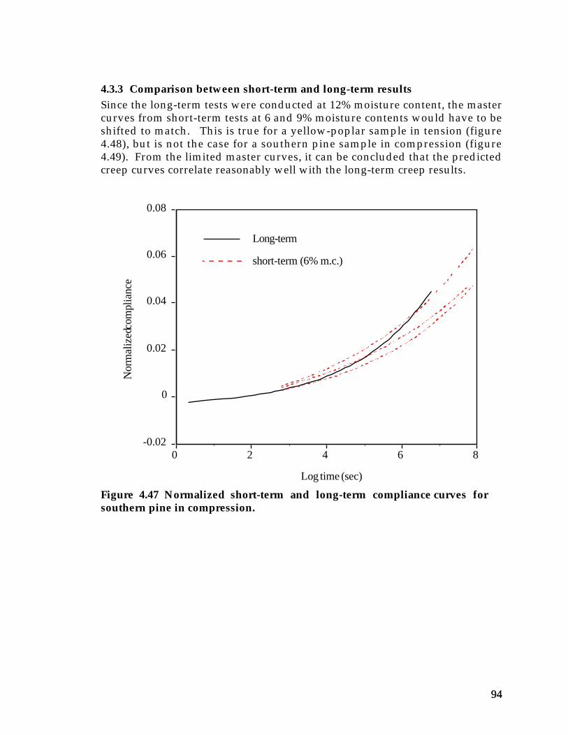
9494

4.3.3 Comparison between short-term and long-term results

Since the long-term tests were conducted at 12% moisture content, the mastercurves from short-term tests at 6 and 9% moisture contents would have to beshifted to match. This is true for a yellow-poplar sample in tension (figure4.48), but is not the case for a southern pine sample in compression (figure4.49). From the limited master curves, it can be concluded that the predictedcreep curves correlate reasonably well with the long-term creep results.

-0.02

0

0.02

0.04

0.06

0.08

Nor

mal

ized

com

plia

nce

0 2 4 6 8

Log time (sec)

short-term (6% m.c.)

Long-term

Figure 4.47 Normalized short-term and long-term compliance curves forsouthern pine in compression.

9595

-0.02

0

0.02

0.04

0.06

0.08

Nor

mal

ized

com

plia

nce

0 2 4 6 8

Log time (sec)

short-term (6% m.c.)

Long-term

Figure 4.48 Normalized short-term and long-term compliance curves foryellow-poplar in tension.

4.4 Finite Element Analysis

A general-purpose finite element program, ABAQUS, was used to analyzevarious simple and complex wood structures such as beams, trusses, arches,and domes.In order to conduct creep analysis in ABAQUS, the user needs to supply acreep model which can be defined in the input data file or in a usersubroutine.

4.4.1 Creep model using time hardening model

A power law in time can be used to define the creep rate as

ε ·cr = A q ˜ n tm (4.1)

where ε ·cr is the uniaxial equivalent creep strain rate, q ˜ is the Mises orHill's equivalent stress (Hill's for anisotropic materials), and A, n, and m areconstants ( A, n > 0, -1 < m ≤ 0 ).The creep behavior is defined in the input file as follows:

9696

*MATERIAL, NAME = A1*ELASTICE, ν*CREEP, LAW = TIMEA, n, m

To model anisotropic creep, the potential option is used to define the ratiosused to scale the stress values in each directions:

*MATERIAL, NAME = A1*ELASTICE, n*CREEP, LAW = TIMEA, n, m*POTENTIALR11, R22, R33, R12, R13, R23

4.4.2 Creep model with user subroutine

An alternative to using the power law to define the creep rate is using asubroutine which is invoked at each integration point. The creep law has thegeneral form

ε ·cr = gcr (p, q, ˜εcr, time,... ) (4.2)

where ε ·cr is the uniaxial equivalent creep strain rate, p is the equivalent

pressure stress p = −1

3 11 + 22 + 33( ) , q ˜ is the Mises or Hill's equivalent

stress (Hill's for anisotropic materials), and εcr is the uniaxial equivalentcreep.The subroutine must define the increments of inelastic creep as functions of

the variables in the gcr function.The subroutine has the following format:

SUBROUTINE CREEP(DECRA,DESWA,ECO,ESWO,P,QTILD,TEMP,DTEMP, 1 PREDEF,DPRED,TIME0,DTIME,STATEV,CMNAME,LEXIMP)C IMPLICIT REAL*8(A-H,O-Z)C CHARACTER*8 CMNAMEC coding to define DECRAC RETURN ENDRequired variables:

DECRA(1): ∆εcr, uniaxial equivalent creep strain increment.Variables needed if implicit integration is used:

DECRA(2): ∂ ∆εcr / ∂ εcr

DECRA(4): ∂ ∆εcr / ∂ p

DECRA(5): ∂ ∆εcr / ∂ q ˜

9797

Example:

If ·cr = A q ˜ tm then

εcr = 1

m+1 A q ˜ t(m +1) at time = t

εcr = 1

m+1 A q ˜ (t+∆t)(m +1) at time = t + ∆T

Therefore

∆εcr = DECRA(1) = 1

m+1 A q ˜ [ ](t+∆t)(m +1) - t(m +1)

and

∂ ∆εcr / ∂ q ˜ = DECRA(5) = 1

m+1 A [ ](t+∆t)(m +1) - t(m +1)

= 1q̃ DECRA(1)

The visco procedureIn order to conduct creep analysis in ABAQUS, the visco procedure is used;the required data input lines are:

*STEP, NLGEOM, INC=200*VISCO, CETOL= ,, EXPLICITinitial time increment,time period,minimum time increment, maximum time increment

4.4.3 Incorporation of the creep law from experimental analysis

The compliance obtained from the creep experiments is fitted to a power lawof the form

D = D0 ( 1 + b tk ) (4.3)

The creep strain can be defined as

εcr = εcr0 b tk

(4.4)

Since εcr0 = σ D0

εcr = σ D0 b tk (5.5)

and the creep strain rate is

ε ·cr= σ kD0 b t(k-1) (5.6)

This equation can be used to obtain the constants A, n, and m used in thecreep law definition in ABAQUS. The constants are:A = kD0 b, n = 1, m = k-1If a user subroutine is used

DECRA(1) = 1

m+1 A QTILD [ ](TIME0+∆ΤΙΜΕ)(m +1) - TIME0(m +1)

DECRA(5) = DECRA(1) / QTILDwhere

QTILD = q ˜

9898

TIME0 = time at the beginning of stepDTIME = time increment

4.4.4 Creep analysis checking

In order to check the creep model used in ABAQUS, the strain measured inone of the tension experiments ( yellow-poplar, 40°C, 12% EMC ) is comparedto that from an ABAQUS finite element analysis. The procedure is asfollows:1) Use nonlinear fitting to obtain the creep parameters; the constants are:

D0 = 5.3732 x 10-7 psi-1

b = 7.0047 x10-3

k= 0.3313which leads to

A = 1.2468 x10-9

n = 1m = -0.6687

2) Use ABAQUS to obtain the creep strain for a period of time comparable tothe duration of the test.

9999

Input file

*HEADING TRUSS ANALYSIS FOR CREEP TISSAOUI*NODE, SYSTEM=R 1, 0.0, 0.0, 2, 7.0 , 0.0*ELEMENT,TYPE=C1D2 ,ELSET=EALL 1 1 2*SOLID SECTION, ELSET=EALL, MATERIAL=WOOD 0.133632*MATERIAL, NAME=WOOD*ELASTIC1.86108E6,0.3*CREEP, LAW=TIME1.246826339E-9, 1.0, -0.6687286*BOUNDARY1,1,32,2,3*STEP, NLGEOM, INC=50*STATIC, PTOL=0.005,DIRECT0.0333, 1.*CLOAD2, 1, 300.0*PRINT, RESIDUAL=NO*EL PRINT, SUMMARY=NO, FREQ=2S,E*NODE PRINT, SUMMARY=NOU,RF,CF*END STEP*STEP, NLGEOM, INC=200*VISCO, CETOL=0.02E-61.0, 22000.0*PRINT, RESIDUAL=NO*EL PRINT, SUMMARY=NO, FREQ=2S,CE*EL FILE, FREQ=1S,CE,E*NODE PRINT, SUMMARY=NOU*NODE FILEU*END STEP

300 lb

As shown in figure 4.49, the strain obtained using ABAQUS is nearlyidentical to that from the creep experiment.

100100

30000200001000001200

1300

1400

1500

ABAQUS

experiment

time [sec]

Stra

in x

106

Figure 4.49 ABAQUS and experimental results for a truss element in tension.

101101

4.4.5 Analysis of a truss for creep

In order to compare long-term creep (50 years) to short-term creep (1 year), aroof truss (figure 4.50) is analyzed using ABAQUS. Gamalath's (1991) creepmodel is used:

Dcr

D0 = P1 tP2

(6.6)

whereP1 = 0.0749 - 2.291 x10-8 E (from regression analysis)P2 = 0.3358 (average)

The parameters for ABAQUS are:

A = P1 P2 D0n = 1m = 1 - P2

3 k

3 k 3 k

4 ft

6 ft 6 ft 6 ft 6 ft

Figure 4.50 Roof truss.

102102

Input file

*HEADING TRUSS ANALYSIS FOR CREEP TISSAOUI*NODE, SYSTEM=R 1, 0.0, 0.0, 2, 72.0, 24.0 3, 144.0, 48.0 4, 216.0, 24.0 5, 288.0, 0.0 6, 144.0, 0.0*ELEMENT,TYPE=C1D2 ,ELSET=EALL 1 1 2 2 2 3 3 3 4 4 4 5 5 2 6 6 4 6 7 1 6 8 5 6 9 3 6*SOLID SECTION, ELSET=EALL, MATERIAL=WOOD 30.25*MATERIAL, NAME=WOOD*ELASTIC2.43140E6,0.3*CREEP, LAW=USER*BOUNDARY1,1,35,2,36,32,33,34,35,3*STEP, NLGEOM, INC=50*STATIC, PTOL=0.005,DIRECT0.0333, 1.*CLOAD2, 2,-3000.03, 2, -3000.04, 2, -3000.0*PRINT, RESIDUAL=NO*EL PRINT, SUMMARY=NO, FREQ=10S,E*NODE PRINT, SUMMARY=NOU,RF,CF*END STEP*STEP, NLGEOM, INC=200*VISCO, CETOL=0.02E-61.0, 4.4E5*PRINT, RESIDUAL=NO*EL PRINT, SUMMARY=NO, FREQ=17S,E*EL FILE, FREQ=10S,*NODE PRINT, SUMMARY=NOU,RF,CF*NODE FILEU*END STEP

103103

Figure 4.51 shows the displacement at the midpoint of the bottom chord

while figure 4.52 shows the percent change in creep u − u0

u0

×100

. After 16

years, the creep displacement is equal to the instantaneous displacement. It isequal to 150 % of the initial displacement after 50 years.

6055504540353025201510500.1

0.2

0.3

0.4

time [years]

Dis

plac

emen

t at

nod

e 6

(in)

Figure 4.51 Displacement at middle of bottom chord

104104

6055504540353025201510500

50

100

150

time [years]

perc

ent

of in

itia

l cre

ep

Figure 4.52 Creep deflection as a percentage of elastic deflection.

105105

4.4.6 Finite element analysis for stability

To illustrate the use of finite element analysis to determine the effect of creepon stability, a small arch and a three-hinged arch are analyzed.Analysis of an archThe arch in figure 4.53 is prone to snap through buckling due to its shallowgeometry. As figure 4.54 shows, the short term buckling load is about 190 lb.When 50% of the short term load is applied, the arch becomes unstable afterabout 70 years as shown in figure 4.55.

30 in

1 in

Hinge

Figure 4.53 Geometry of the A-frame (cross sectional area = 1 in2).

1.00.80.60.40.20.00

50

100

150

200

Vertical displacement at the apex [in]

Concentr

ate

d load a

t th

e a

pex

[lb]

Figure 4.54 Load deflection path at the apex.

106106

807060504030201000.0

0.1

0.2

0.3

0.4

0.5

0.6

Time [years]

Apex v

ert

ical dis

pla

cem

ent

[in]

Figure 4.55 Long term response of the frame under 50% of short term criticalload.

107107

Creep of a three hinged arch

Figure 4.56 shows a three hinged arch that was used as a design example byFaherty and Williamson (1989). The design loads were 400 lb/ft dead load and480 lb/ft snow load. The arch cross section is 6.75 x 27 in. ABAQUS was usedto determine the long-term behavior of the arch . The creep law proposed byNielsen (1992) was used. Figure 4.57 shows the deflection at the apex vs. timefor dead load in combination with uniform snow load and snow over halfthe arch. The arch does not become unstable after 50 years, this is due to thelarge safety factor against buckling. The short term critical loads anddeflections are:Uniform snow load: Pcr = DL + 4.88 LL

∆cr = 16.26 in at apexHalf snow load: Pcr = DL + 6.791 LL

∆cr = 30.16 in at apex

108108

100 ft

Hinge

13.3975 ft

6.75 in

27 in

(a) (b)

Figure 4.56 (a) Geometry and (b) cross section of three hinged arch

60504030201000

1

2

3

4

time [years]

Dis

pla

cem

ent

at

apex

[in]

uniform snow load

half snow load

Figure 4.57 Creep displacements at the apex.

Creep of the Church of the Nazarene Varax DomeThe Varax dome dimensions are shown in figure 4.58 The dome consists ofseven identical sectors and is supported by fourteen columns. At theperimeter, a steel ring with a cross-sectional area of 5 in2 provides additionalsupport (Tissaoui, 1991). The dome consists of 77 beams (5.125 x 12 in), 112purlins (3.125 x 7.5 in), and 14 edge beams (3.125 x 22 in). The beams are

109109

connected using the Varax connector. The dome is covered with 2-in tongue-and-groove wood decking which is not included in this model to simplify theanalysis. The design loads for the dome are 15 psf dead load and 25 psf snowload.

110110

22.4 ft

130.7 ft

Figure 4.58 Varax dome geometry.

From static nonlinear analysis, it was determined that the critical load factorfor the live load is equal to 3.32. The vertical displacement at the apex wasbetween 2.5 and 3.0 in. The buckled shape is shown in figure 4.59.

111111

Figure 4.59 Buckled shape of the dome

Creep analysis was conducted for 50 years, using creep laws from Gamalath(1991), LeGovic (1987), and the equations from our long-term tests. Theparameters used are shown in table 4.7.

Table 4.7 Creep parameters used in finite element analysis of the Varaxdome.

Le Govic Gamalath long-term (southern pine)D0 (in2/lb) 4.045x10-7 4.113 x10-7 5.545 x10-7

b sec-k 0.0388 0.0192 0.0154k 0.112 0.3358 0.1373

112112

The snow load was applied for the entire 50 years which, although unrealistic,is a worst case assumption which may reveal potential instability. Figure 4.60shows the vertical displacement at the apex. In the worst case, thedisplacement doubled, but no instability was detected.

0.75

1

1.25

1.5

1.75

2V

ertic

al d

ispl

acem

ent a

t the

ape

x (i

n)

0 10 20 30 40 50 60

time (years)

long-term

Le Govic (1987)

Gamalath (1991)

Figure 4.60 Vertical displacement at the dome apex.

From the above results, it is clear that creep will not lead to instability duringthe design life of the Varax dome.

113113

5. CONCLUSIONS AND RECOMMENDATIONS

5.1 Conclusions

The application of the principle of time-temperature superposition was onlypossible at temperatures below 65°C, and the resulting creep curves did notextend beyond 2 years. As was determined from the dynamic tests and fromthe literature (Kelly et al, 1987), wood undergoes two distinct transitions dueto lignin and hemicellulose. These transitions depend on the moisturecontent. This would make wood thermorheologically complex having two ormore phases; additionally, if the lignin and hemicellulose depend differentlyon temperature, one would expect wood to exhibit different responsesdepending on where it is in the time/temperature/moisture content scale.The breakdown of TTSP for thermorheologically complex polymers is welldocumented (Fesko and Tschoegl 1971, 1974, Lim et al., 1971). TTSP is notapplicable to a block copolymer unless one of the components dominates thebehavior. When neither component dominates, each contributes differentlyto the behavior and the curves cannot be superposed. Between 6 and 12%moisture content, wood undergoes transitions due to either or bothhemicellulose and lignin between 65 and 80°C. During and after thistransition, the behavior changes and TTSP can no longer be applied.Therefore, TTSP can be only be applied at temperatures below 70°C, theresulting horizontal shift factors follow an Arrhenius relation with activationenergies between 75 and 130 kJ/mole. The response can be extended furtherthan 2 years by extending the creep test at 60°C to a week or more.

It was not possible to determine whether Parallam™ is more susceptible tocreep than solid wood. This can be attributed to the small size of the samplesused.

The power law equation for creep can be used in finite element analysis tomodel the long term behavior of wood structures. Serviceability andinstability problems can be predicted. From finite element analysis of theVarax dome subjected to dead and snow loads, it can be concluded that creepdoes not lead to instability during the design life.

5.2 Recommendations

• At the maximum temperature (60 or 65°C), the test should be conducted fortwo days to a week to obtain a master curve that extends for more than adecade. Then the sample should be tested again at the lowest temperature tocheck for damage, as was done by Colby (1989).

114114

• Creep experiments on wood are very sensitive to temperature and relativehumidity changes, and rate of loading. Also the tests are time consuming andrequire daily monitoring. Automating the tests would make the task easierand less demanding. The tests can be automated by using a computer tocontrol loading and unloading of the samples, temperature and relativehumidity increases, monitoring of the moisture contents of the samples, anddata collection and manipulation. • A computer program can be written or purchased to automaticallysuperpose the individual creep curves. This would lead to elimination ofoperator bias, also more data can be processed in less time.• The dynamic behavior at a wide range of temperatures and frequencies andat different moisture contents should be studied further.• Larger samples of Parallam™ and other structural lumber compositesshould be tested to determine if they are more susceptible to creep.

115115

6. REFERENCES

ABAQUS, General-Purpose Finite Element System , Hibbit, Karlsson andSorensen, Inc., 100 Medway Street, Providence, RI 02906, USA.

American Institute of Timber Construction, Timber Construction Manual ,third editions, John Wiley & Sons, Inc., New York, 1985.

Aklonis, J. J., and MacKnight, W. J. , Introduction to Polymer Viscoelasticity ,John Wiley and Sons, 1983.

Bathe, K. J. , Finite E lement Procedures in Engineering Analysis , Prentice-Hall, Englewood Cliffs, N.J., 1982.

Bodig, J., and Jayne, B. A., Mechanics of Wood and Wood Composites , VanNostrand Reinhold Company, 1982.

Bodig (ed.), J. , Reliability-Based Design of Engineered Wood Structures ,Kluwe Academic Publishers, 1992.

Bond, B. H., Development of Tension and Compression Creep Models forWood Using the Time-Temperature Superposition Principle. Thesis (M.S.)--Virginia Polytechnic Institute and State University , 1993.

Boyle, J. T., and Spence, J., Stress Analysis of Creep , Butterworths, 1983.

Britvec, S. J., The Stability of Elastic Systems , Permagon Press Inc, 1973.

Bushnell, D., "A Strategy for the Solution of Problems involving LargeDeflections, Plasticity, and Creep," International Journal for Numerical Methods in Engineering , Vol. 11, 1977, pp. 683-708.

Chan, E. C. Y., "Nonlinear Geometric, Material, and Time DependentAnalysis of Reinforced Concrete Shells with Edge Beams," Ph.D. Dissertatio n ,University of California, Berkeley, 1983.

Chang, Y.S., Personal communication, 1991.

Clauser, W. S., "Creep of Small Wood Beams Under Constant Bending Load," Forest Products Laboratory, Forest Service U.S.D.A. , Report No. 2150, 1959.

116116

Colby, R. H., “Breakdown of time-temperature superposition in MisciblePolymer Blends,” Polymer , 1989, 0Vol. 30, pp. 1275-1278.

Davidson, R. W. , "The Influence of Temperature on Creep in Wood," Forest Products Journal , 1962, pp377-381

Desh, H. E. , Timber, its Structure, Properties and Utilisation , Timber Press,1981.

Dinwoodie, J. M. , Wood: Nature's Cellular, Polymeric, Fibre-Composite , TheInstitute of Metals, 1989.

Emri, I. and Pavsek V., "On the Influence of Moisture on the MechanicalProperties of Polymers," Materials Forum , 1992, vol. 16, pp. 123-131.

Faherty, K. F. , Williamson, T. G. , Wood Engineering and Construction Handbook , McGraw Hill-Inc, 1989.

Ferry, J. D. , Viscoelastic Properties of Polymers , John Wiley and Sons, 1980.

Fesko, T. G. and Tschoegl, N. W. , "Time-Temperature Superpostion inThermorheologically Complex Materials," Journal of polymer science. Part C, Polymer letters , 1971, No. 35, pp. 51-69

Fesko, T. G. and Tschoegl, N. W. , "Time-Temperature Superpostion inStyrene/Butadiene Block Copolymers," International Journal of Polymeric Materials , 1974, Vol. 3, pp. 55-79

Findley, W. N., “Creep Characteristics of Plastics,” Proc. Symposium on Plastics , American Society for Testing and Materials, Philadelphia, PA, 1944,pp118-34.

Gamalath, S. , "Long Term Creep Modeling of Wood Using Time-Temperature Superposition Principle," Ph.D. Dissertation . Wood Science andForest Products, Virginia Polytechnic Institute & State University, Virginia,USA, 1991.

Greenbaum, G. A. , and Rubinstein, M. F. , "Creep Analysis of AxisymmetricBodies using Finite Elements," Nuclear Engineering and Design , Vol. 7, 1968,pp. 379-397.

117117

Gressel, P. , "Prediction of Long-Term Deformation Behavior from Short-Term Creep Experiments," Holz als Roh- und Werkstoff , Vol. 42, 1984, pp.293-301.

Hermida, E. B. and Povolo F., "Analytical-Numerical Procedure toDetermine if a Set of Experimental Curves Can Be Superimposed to Form aMaster Curve," Polymer Journal , Vol. 26, No. 9 pp 981-992 (1994).

Holzer, S. M. ,Loferski, J. R. , and Dillard, D. A. , "A Review of Creep inWood: Concepts Relevant to Develop Long-Term Behavior Predictions forWood Structures," Wood and Fiber Science , 21(4), 1989, pp. 376-392.

Huet, C. , and Navi, P. , "Multiparabolic Multitransition Model for Thermo-Viscoelastic Behavior of Wood," Mechanics of Wood and Paper Materials,AMD-Vol 112, 1990, pp. 17-24.

Irvine, G. M., “The Glass Transition of Lignin and Hemicellulose and theirMeasurement by Differential Thermal Analysis,” Tappi Journal , May, 1984,pp. 118-121.

Kabir, A. F., "Nonlinear Analysis of Reinforced Concrete Panels, Slabs andShells for Time dependent Effects," Ph.D. Dissertation . Civil Engineering,University of California, Berkeley, USA, 1976.

Kelly, S. S., Rials, T. G. , and Glasser, W. G , "Relaxation Behaviour of theAmorphous Components of Wood," Journal of Material Science , 1987, pp22:617-624

Kraus, H. , Creep Analysis , Wiley, 1980.

Le Govic, C. , Felix, B. , Hadj Hamou, A. , Rouger, F. , and Huet, C. ,"Evidence for an Equivalence Between Time and Temperature and ModelingCreep in Wood," Actes du 2e colloque. Sciences et industries du bois , Nancy,22-24 avril, 1987, pp I:349-356.

Le Govic, C. , Felix, B. , Benzaim, A. , and Rouger, F. , "Creep Behavior ofWood as a Function of Temperature: Experimental Study, Modelling andConsequences for Design Codes," Proceedings of the Second Pacific Timber Engineering Conference , University of Auckland, New Zeland, 28-31 August,1989, pp. 273-277.

118118

Lim, C. K., Cohen, R.E., and Tschoegl, N. W., “Time-TemperatureSuperposition in Block Copolymers,” Advances in Chemistry Series , ACSMonograph No. 99, 1971, pp. 397-417.

McCrum, N. G. ,and Morris, E. L. , "On the Measurement of the ActivationEnergies for Creep and Stress Relaxation," Proc. Roy. Soc. , 1964, Vol. 281

Mendelson, A. , and Hirschberg, M. H. , and S. S. Manson, "A GeneralApproach to the Practical Solution of Creep Problems," Journal of Basic Engineering , ASME, Vol. 81, 1959, pp. 585-598.

Nakayasu, H. , Markovitz, H., Plazek, D. J., "The frequency and TemperatureDependence of the Dynamic Mechanical Properties of a Hign DensityPolyethylene," Transactions of The Society of Rheology, 1961, pp. 261-283.

National Design Specifications for Wood Construction, National Forest Products Association , 1986, Washington, D.C.

Neal, D. W. , "Restoration of Navy LTA (Lighter than Air) Hangars,"Evaluation and Upgrading of Wood Structures: Case Studies, Proceedings Structures Congress '86 , ASCE, September 1986, pp. 1-12.

Nickell, R. E. , "Thermal Stress and Creep," in Structural Mechanics Computer Programs , W. D. Pilkey et al., editors, University Press of Virginia,Charlottesville, 1974, pp. 103-122.

Nielsen, L. F. , "Power Law Creep as Related to Relaxation Elasticity,Damping, Rheological Spectra, and Creep Recovery - with Special Referenceto Wood," IUFRO Timber Engineering Group Meeting , Xalapa, Mexico1984.

Nielsen, L. F. , "Lifetime of Wood as Related to Strength Distribution," Reliability-Based Design of Engineered Wood Structures , Bodig, J. (ed.),Kluwe Academic Publishers, 1992.

Nilson, A. H. , et al., Finite Element Analysis of Reinforced Concrete ,American Society of Civil Engineers, 1982.

Onogi, S., Sasaguri, K., Adachi, T., Ogihara, S., "Time-HumiditySuperposition in Some Crystalline Polymers," Journal of Polymer Science,1962, Vol. 58, pp. 1-17.

119119

Oviatt, A. E. Jr., "Moisture Content of Glulam Timbers in Use in the PacificNorthwest," Pacific Northwest Forest and Range Experiment Station, ForestService, U.S.D.A., 1968.

Plazek, D. J., “Temperature Dependence of the Viscoelastic Behavior ofPolystyrene,” The Journal of Physical Chemistry , 1965, v 69 pp 480-487.

Povolo, F., and Fontelos, N. , "Procedure to Determine if a set of ExperimentalCurves are Really Related by Scaling," Res Mechanica, Vol. 22, 1987, pp. 185-198.

Sakata, I. , and Senju, R. , "Thermoplastic Behavior of Lignin with VariousSynthetic Plastisizers," Journal of Applied Polymer Science , 19pp19:2799-2810

Salmèn, N. L., "Viscoelastic Properties of in Situ Lignin Under Water-Saturated Conditions," Journal of Material Science , 1975, pp10:3090-3096

Schniewind, A. P., "Recent Progress in the Study of the Rheology of Wood."Wood Science and Technology, Vol 2, 1968, pp 188-206.

Sharma, M. G. , "Theories of Phenomenological Viscoelasticity UnderlyingMechanical Testing," Testing of Polymers , Schmitz, J. V. (ed.), IntersciencePublishers, 1965, pp. 147-199.

Simpson, W. T., “Equilibrium Moisture Content Prediction for Wood.” Forest Products Journal , 1971, Col. 21, pp 48-49.

Snyder, M. D. and Bathe, K. J. , "A Solution Procedure for Thermo-Elastic-Plastic and Creep Problems," Nuclear Engineering and Design , Vol. 64, 1981,pp. 49-80.

Takayanagi, M. , "Viscoelastic Behavior of Crystalline Polymers," FourthInternational Congress on Rheology, Vol. 1, Interscience, New York, 1965, pp.161-187

Tissaoui, J., “StabilityAnalysis of the Church of the Nazarene Varax Dome”,M.S. Thesis. Civil Engineering , Virginia Polytechnic Institute & StateUniversity, Virginia, USA, 1991.

Tissaoui, J., Loferski, J. R., Holzer, S. M., Dillard, D. A., Bond, B. H.,

120120

“Long-term creep law for wood in compression and tension parallel to grain,” Mechanics of Cellulosic Materials , American Society of Mechanical Engineers,Applied Mechanics Division, v 145, pp 33-38

Van Der Put, T. A. C. M. , "Deformation and Damage Processes in Wood,"Delft University Press, 1989.

Yen, S. , and Williamson, F. L. , "Accelerated Characterization of CreepResponse of an Off-Axis Composite Material," Composites Science and Technology , Vol. 38, 1990, pp. 103-118.Williams, J. G., Stress Analysis of Polyme rs , John Wiley and Sons, 1980.

Wolcott, M. P., "Modeling Viscoelastic Cellular Materials for the Pressing ofWood Composites," Ph.D. Dissertation. Materials Engineering Science ,Virginia Polytechnic Institute & State University, Virginia, USA, 1989.

Wood Handbook , United States Department of Agriculture, U.S. ForestProducts Laboratory, Agriculture Handbook No. 72, U.S. GovernmentPrinting Office, Washington, D.C., 1987.

Zienkiewicz, O. C., The finite Element Method in Engineering Science ,MaGraw-Hill, London, 1971

Zienkiewicz, O. C. , and Cormeau, I. C. , "Viscoplasticity-Plasticity and Creepin Elastic Solids - A United Numerical Approach," International Journal for Numerical Methods in Engineering , Vol. 8, 1974, pp. 821-845.

Zienkiewicz, O. C. , and Watson, M. , "Some Creep Effects in Stress Analysiswith Particular Reference to Concrete Pressure Vessels," Nuclear Engineering and Design , Vol. 4, 1966, pp. 406-412.

121121

Vita

Jacem Tissaoui was born in Jendouba, Tunisia on December 5, 1967. Hefinished high school in 1985 after which he came to the United States topursue a Bachelor of Science degree in Civil Engineering at Penn State. Aftergraduating in 1989, he attended Virginia Tech where he obtained a Master ofScience degree in Civil engineering and continued to pursue a PhD degree.He was married in 1992 to Luz and had a son, Yassine in 1994. Aftergraduating he plans to go home to Tunisia.