Effects of overstory mortality on snow accumulation and ablation

Patrick Teti

Mountain Pine Beetle Working Paper 2008-13

B.C. Ministry of Forests and Range

200 – 640 Borland St.

Williams Lake, BC V2G 4T1

MPBI Project # 8.39

Natural Resources Canada Canadian Forest Service Pacific Forestry Centre

506 West Burnside Road Victoria BC V8Z 1M5

2008

© Her Majesty the Queen in Right of Canada 2008

Printed in Canada

Library and Archives Canada Cataloguing in Publication

Teti, Patrick Anthony, 1949- Effects of overstory mortality on snow accumulation and ablation / Patrick Teti.

(Mountain Pine Beetle Initiative working paper 2008-13) "MPBI Project # 8.39". Includes bibliographical references: p. Includes abstract in French. ISBN 978-1-100-10636-6 Cat. no.: Fo143-3/2008-13E

1. Forest hydrology--British Columbia. 2. Snow surveys--British Columbia. 3. Forest surveys--British Columbia. 4. Forests and forestry--Environmental aspects--British Columbia. 5. Forest ecology--British Columbia. 6. Mountain pine beetle--British Columbia. 7. Pine--Diseases and pests--British Columbia. I. Pacific Forestry Centre II. Title. III. Series.

SB945.M78H46 2008 551.57'971109152 C2008-980326-4

ii

Abstract Total annual runoff and peak streamflows from watersheds draining B.C.’s Interior Plateau are largely driven by spring snowmelt, which in turn is influenced by the condition of forests. Those forests are dominated by Lodgepole pine and are undergoing rapid change due to the mountain pine beetle epidemic. This project has documented physical stand characteristics, snow accumulation, and snow ablation rates of growing managed stands and deteriorating natural stands in six groups of plots. Thirty-six long-term research plots were established in six groups in the Vanderhoof, Quesnel, Chilcotin, Central Cariboo, and Kamloops Forest Districts. Plot characteristics were documented by doing detailed tree and coarse woody debris surveys, and by taking fisheye canopy photos from which solar radiation transmittances and other optically-derived parameters were calculated. Snow accumulation and ablation rates were documented by ground surveys and aerial photography in 2006 and 2007. In four of the six groups, where snow accumulation data are considered most reliable, snow water equivalents were highest in plots that had been clearcut or burned in a wildfire within the last 10 years. Snow accumulation was lowest in old foliated stands and managed stands greater than 25 years old. Accumulation in beetle-attacked stands relative to nearby cutblocks less than 10 years old ranged from 77% (Rosita) to 90% (Vanderhoof). Also in four of the six groups, snow ablation rates were highest in stands that had been logged less than 15 years earlier. Ablation rates in managed stands more than 30 years old were similar to those in old intact forests. These results suggest that logging dead pine stands will increase the total amount and rate of spring snowmelt over what would have otherwise occurred for about 15 years. Keywords: mountain pine beetle, snow hydrology, hydrologic recovery, forest canopy, transmitted solar radiation

iii

Résumé

Le volume annuel et l’écoulement fluvial maximal des bassins hydrographiques drainant le plateau intérieur de la Colombie-Britannique proviennent largement de la fonte des neiges, laquelle dépend de l’état des forêts. En Colombie-Britannique, les forêts sont dominées par le pin tordu et subissent des changements rapides en raison de l’épidémie de dendroctone du pin ponderosa. Le projet a documenté les caractéristiques des peuplements, l’accumulation de neige, les taux d’ablation nivale des peuplements gérés en croissance et la détérioration des peuplements naturels de six groupes de parcelles. Trente-six parcelles utilisées pour la recherche à long terme forment ces six groupes dans les districts forestiers de Vanderhoof, Quesnel, Chilcotin, Cariboo-Centre et Kamloops. Les caractéristiques des parcelles ont été documentées à l’aide de levés détaillés des arbres et des débris forestiers grossiers et de photographies du couvert forestier à angles extrêmes à partir desquelles nous avons calculé la transmission du rayonnement solaire et d’autres paramètres de nature optique. L’accumulation de neige et les taux d’ablation nivale ont été documentés à l’aide de levés au sol et de photographies aériennes réalisés en 2006 et 2007. Pour quatre des six groupes, pour lesquels nous considérons que les données d’accumulation de neige sont fiables, l’équivalent en eau de la neige est le plus élevé dans les parcelles qui ont été coupées à blanc ou brûlées dans un incendie de forêt au cours des 10 dernières années. L’accumulation de neige était la plus faible dans les peuplements feuillus âgés et les peuplements gérés de plus de 25 ans. L’accumulation de neige dans les peuplements attaqués par le dendroctone relativement aux blocs de coupe de bois de moins de 10 ans allait de 77 % (Rosita) à 90 % (Vanderhoof). De plus, dans quatre des six groupes, les taux d’ablation nivale étaient plus élevés dans les peuplements ayant été moins exploités dans les dernières 15 années. Les taux d’ablation nivale dans les peuplements gérés de plus de 30 ans étaient comparables à ceux des peuplements dans des forêts âgées non altérées. Ces résultats suggèrent que l’exploitation des peuplements de pins morts augmente le volume total et le taux de fonte des neiges; un processus qui aurait autrement exigé une quinzaine d’années. Mots-clés : dendroctone du pin ponderosa, hydrologie nivale, récupération hydrologique, couvert forestier, transmission du rayonnement solaire

iv

Table of Contents

1 Introduction..........................................................................................................................1 1.1 Overview..................................................................................................................1 1.2 Rationale ..................................................................................................................1

2 Materials and Methods.........................................................................................................2 2.1 Plot Establishment ...................................................................................................2 2.2 Snow Surveys...........................................................................................................2 2.3 Coarse Woody Debris Surveys ................................................................................3 2.4 Fisheye Canopy Photography ..................................................................................3

2.4.1 Acquisition and Analysis 3 2.4.2 Comparison of methods for estimating radiation from fisheye photos 5

2.5 Tree Surveys ............................................................................................................6 2.6 Aerial photography ..................................................................................................6

3 Results and Discussion ........................................................................................................7 3.1 Snow Accumulation.................................................................................................7 3.2 Stem densities, crown characteristics, and transmitted radiation ............................9 3.3 Diffuse Radiation and Sky View Factor ................................................................11 3.4 Variability of transmitted radiation within plots....................................................12 3.5 Ablation rates and transmitted radiation ................................................................13

4 Conclusions........................................................................................................................14

5 Acknowledgements............................................................................................................15

6 Literature Cited ..................................................................................................................15

v

vi

List of Tables

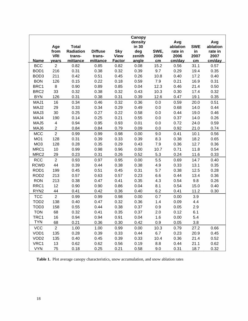
Table 1. Plot average canopy characteristics, snow accumulation, and snow ablation

rates ........................................................................................................................... 18 Table 2. Parameters used in Gap Light Analyzer ............................................................ 19

List of Figures Figure 1. Locations of plot groups................................................................................... 20 Figure 2. Regions of the celestial hemisphere in which gap fractions were calculated... 21 Figure 3. Hourly incoming direct radiation under clear skies on April 9th at 52 degrees

north latitude ............................................................................................................. 22 Figure 4. Above canopy diffuse radiation as a function of zenith angle ......................... 22 Figure 5. Comparison of total radiation transmittances calculated for individual

hemispherical photos by GLA and the Rosita method ............................................. 23 Figure 6. Arrangement of fixed radius tree survey plots within a snow research plot using

the 7.98 metre radius (200 square metre) plot as an example................................... 24 Figure 7. Snow accumulation ratios versus canopy densities in all plots........................ 24 Figure 8. Snow accumulation ratios vs canopy density in each group ............................ 25 Figure 9. Plot average snow accumulation ratios versus stand ages................................ 26 Figure 10.Plot average canopy densities versus stand age ............................................... 26 Figure 11. VYN, a 75 year-old natural stand…………………………………………….27 Figure 12. MRC2, a 30 year-old managed stand………………………………………...27 Figure 13. RON, a 213 year-old natural stand…………………………………………...27 Figure 14. ROD2, a 213 year-old natural stand, heavily attacked by beetles in 1980.......27 Figure 15a.Plot average radiation transmittance versus stand age from the VRI, except

plot TON, which is estimated to be at least 130 years old…...…………...………..28 Figure 15b.Same data as Figure 12a, showing the data grouped into young managed

stands, young natural stands, and old stands……………………………………….28 Figure 16a.Plot MO1 in April 2006...………………………………………….………..29 Figure 16b.Plot MO1 in April 2007……………………………………………………..29 Figure 17. Plot average diffuse versus total radiation transmittances in all plots……….30 Figure 18. Plot average sky view factors versus total radiation transmittances in all

plots………………………………………………………………………………...30 Figure 19. One-sided ninety-five percent confidence limits on the estimate of mean

radiation transmittances in each plot versus sample size…………………………..31 Figure 20. Plot average radiation transmittances versus plot average Angular Canopy

Gaps obtained from fisheye photos………………………………………………...31 Figure 21a. Plot average ablation rates in 2006 versus average radiation transmittances 32 Figure 22b. Plot average ablation rates in 2007 versus average radiation transmittances 33

1 Introduction

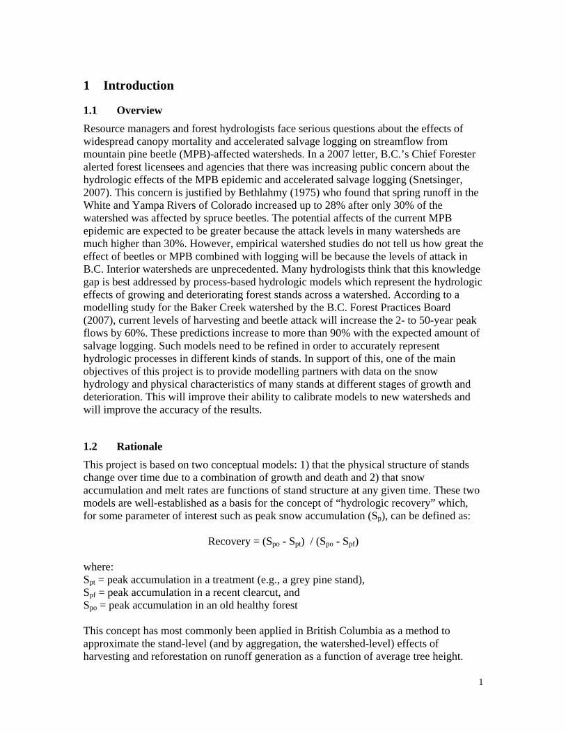
1.1 Overview Resource managers and forest hydrologists face serious questions about the effects of widespread canopy mortality and accelerated salvage logging on streamflow from mountain pine beetle (MPB)-affected watersheds. In a 2007 letter, B.C.’s Chief Forester alerted forest licensees and agencies that there was increasing public concern about the hydrologic effects of the MPB epidemic and accelerated salvage logging (Snetsinger, 2007). This concern is justified by Bethlahmy (1975) who found that spring runoff in the White and Yampa Rivers of Colorado increased up to 28% after only 30% of the watershed was affected by spruce beetles. The potential affects of the current MPB epidemic are expected to be greater because the attack levels in many watersheds are much higher than 30%. However, empirical watershed studies do not tell us how great the effect of beetles or MPB combined with logging will be because the levels of attack in B.C. Interior watersheds are unprecedented. Many hydrologists think that this knowledge gap is best addressed by process-based hydrologic models which represent the hydrologic effects of growing and deteriorating forest stands across a watershed. According to a modelling study for the Baker Creek watershed by the B.C. Forest Practices Board (2007), current levels of harvesting and beetle attack will increase the 2- to 50-year peak flows by 60%. These predictions increase to more than 90% with the expected amount of salvage logging. Such models need to be refined in order to accurately represent hydrologic processes in different kinds of stands. In support of this, one of the main objectives of this project is to provide modelling partners with data on the snow hydrology and physical characteristics of many stands at different stages of growth and deterioration. This will improve their ability to calibrate models to new watersheds and will improve the accuracy of the results.

1.2 Rationale This project is based on two conceptual models: 1) that the physical structure of stands change over time due to a combination of growth and death and 2) that snow accumulation and melt rates are functions of stand structure at any given time. These two models are well-established as a basis for the concept of “hydrologic recovery” which, for some parameter of interest such as peak snow accumulation (Sp), can be defined as:

Recovery = (Spo - Spt) / (Spo - Spf) where: Spt = peak accumulation in a treatment (e.g., a grey pine stand), Spf = peak accumulation in a recent clearcut, and Spo = peak accumulation in an old healthy forest This concept has most commonly been applied in British Columbia as a method to approximate the stand-level (and by aggregation, the watershed-level) effects of harvesting and reforestation on runoff generation as a function of average tree height.

1

This simplified representation of stand structure has been justified by the convenience of using a simple parameter for operational purposes and by the fact that managed stands have simpler structures than natural stands. While clearcut equivalency is often used as a basis for comparing the relative effects of beetles and logging, it is of limited value for predicting changes in actual peak flows. Process-based watershed runoff models are needed for this purpose and they require quantitative estimates of physical parameters that affect water and energy budgets. Therefore, this project is providing watershed modelling partners with estimates of physical stand parameters in addition to snow accumulation and ablation curves. This is particularly important for unsalvaged beetle-attacked stands because they are more complex than managed stands and because their physical features have not been well-quantified in the past.

2 Materials and Methods

2.1 Plot Establishment Six groups of plots were established across a broad portion of the Interior Plateau in BEC zones that have been severely impacted by the recent MPB epidemic. Three groups are in the SBPS, two are in the MS, and one is in the SBS biogeoclimatic zone. The goal within each group was to minimize the effects of geography and maximize the diversity of stand types represented. All plots are on slopes of 7% or less and within each group, all plots are within 6.4 km horizontal distance and 65 m elevation of each other. Figure 1 shows the locations of the six groups and Table 1 lists their geographic characteristics. Each of the 24 new plots established under this project (the Vanderhoof, Baker, Rosita, Taseko, and Moffat groups) were installed as a 6 × 6 grid with points spaced at 10 m intervals over an area of 50 × 50 m. Permanent points were marked with steel rebar to which bamboo poles were attached. The resulting 36 points constituted the spatial sample for all snow measurements and hemispherical photography. The locations of plot corners were determined by GPS to a horizontal accuracy of 10 m. The project was registered as EP 1371 with the B.C. Ministry of Forests and Range Research Branch. Regular contact was made with forest licensees in order to protect the plots from logging, pending its declaration as a “Resource Feature” under the Government Actions Regulation. The Mayson Lake group of plots had been previously established by Dr. Rita Winkler with 24 to 36 points per plot.

2.2 Snow Surveys In the spring of 2006 and 2007, snow was surveyed in each of the 24 plots in the Vanderhoof, Baker, Rosita, Taseko, and Moffat groups by a non-standard method in order to minimize costs. This consisted of doing one detailed snow survey on the ground at the time of estimated maximum snowpack (estimated by doing reconnaissance snow surveys) and repeated fixed wing aerial surveys in order to estimate the date of snow

2

disappearance in each plot. It was assumed that the date on which snow storage dropped to zero could be approximated by the date on which the portion of ground covered by snow dropped to 50%. This is supported by results from five years of monitoring snow in the ESSF (Teti 2003). Using this method, peak snow storage and average snow ablation rates were estimated for each plot in the spring of 2006 and 2007. In the Mayson Lake group of plots, peak storage and ablation rates were calculated by the standard method of repeated detailed ground surveys.

2.3 Coarse Woody Debris Surveys In the summer of 2006, coarse woody debris was surveyed on all plots in the Vanderhoof, Baker, Rosita, Taseko, and Moffat groups by measuring wood diameters, heights above ground, and decay classes under four 35.4 m lines (line-intercept) within each plot. These methods were similar to those of Densmore, et al. (2004).

2.4 Fisheye Canopy Photography 2.4.1 Acquisition and Analysis Hemispherical canopy photos were taken at all points in all 36 plots in the summer of 2006. A Nikon Coolpix 4500 digital camera with Nikkor FC-E8 auxiliary fisheye lens was used at a height of 1.1 m above ground. Photos were analyzed with Gap Light Analyzer (Frazer et al. 1999) and a method developed by the project leader. Several canopy parameters were calculated including one that affects snow interception (canopy density within a 30° zenith angle), two that regulate the transfer of long wave radiation between the snow and overhead emitters/absorbers (sky view factor, canopy view factor), and two that regulate the amount of incoming shortwave radiation available to the snowpack (percent transmittances of incoming direct and diffuse solar radiation through the canopy). Photos were taken at every point except in the recent clearcuts where photos were taken only in the four corners due to the near absence of measurable canopy in those plots. Lens geometry had been previously documented by photographing a room in which the walls and ceiling had been marked at the intersections of polygons in 10° increments of zenith angle and 45° increments of azimuth. The calibration room was also marked with sun positions in one-hour increments from 0800 to 1600 local solar time for seven equatorial declinations corresponding with July 1st and June 10th, August 1st and May 10th, August 15th and April 26th, September 1st and April 9th, September 15th and March 26th, October 1st and March 10th, October 15th and February 24th. Sun positions corresponding with these dates and times were obtained for 52° north from NASA’s Jet Propulsion Laboratory solar ephemeris (http://ssd.jpl.nasa.gov). Photos were taken with the camera at a height of 1.1 m above ground on a Manfrotto tripod having a built-in level. By taking repeated photos in the calibration room, this

3

method was found to have a zenith positioning accuracy of approximately 3°. Azimuthal orientation of photos was determined by holding a visible target north of the camera while taking each photo. Several authors have recommended taking canopy photos only under overcast skies in order to best discriminate between sky and canopy features (e.g. Frazer et al. 2001). However, this was impractical because skies are seldom uniformly overcast during the summer. Most photos were taken under clear or partly cloudy skies. When the camera lens was in direct sunlight it was shaded with a paddle on the end of a stick. When the paddle was not used, diffuse sunlight sometimes caused local overexposure resulting in under-representation of canopy around the sun. Another occasional problem was direct sunlight illuminating tree boles, branches, and foliage which caused some misclassification of canopy as sky. Photos were retouched to remove or add canopy or sky as deemed necessary. Each image was processed as follows: 1) register it to the image taken in the calibration room using Adobe Photoshop, 2) re-touch as described above, 3) categorize all pixels as sky or canopy using Sidelook (Nobis and Hunziker 2005), 4) calculate gap fractions in each of 65 regions in equal increments of altitude and azimuth with a user-written macro in Scion Image for Windows (Scion Corporation http://www.scioncorp.com/), 5) with another Scion macro, calculate gap fraction in each of 48 sky regions corresponding with sun positions during six periods of the year from February 24th to June 10th (also corresponding with July 1st to October 15th ). The regions of sky for which gap fractions were calculated are shown in Figure 2. Gap fractions were averaged in each of nine annuli in 10° zenith angle increments and sky view factors were calculated to a horizontal surface using the method described by Steyn (1980). Average gap fractions within these zenith angle bands were also the basis for calculating transmitted diffuse solar radiation as described below. Hourly average percent transmittances of direct radiation in different seasons were obtained directly from gap fractions along solar paths shown in Figure 2. Hemispherical radiation models for direct and diffuse radiation above the canopy were developed for cloud-free conditions on April 9th using Gap Light Analyzer. This combination of conditions was selected because both high snow storage and high snowmelt rates can occur on the Fraser Plateau in early April. The atmospheric parameters were chosen to represent springtime radiation under clear skies, when high melt rates are likely to occur. Input parameters used for Gap Light Analyzer (GLA) are shown in Table 2. Gap Light Analyzer provides an option to calculate incoming and transmitted direct and diffuse radiation in small increments of altitude and azimuth for the entire hemisphere. However, we wanted a model of incoming direct radiation as functions of date and time to be compatible with our sun path coordinates in Figure 2 and to make the results more easily compared with radiation models based on time of day. In order to obtain direct radiation for April 9th in one-hour increments, daily direct transmitted radiation was calculated with GLA for a set of artificial hemispherical images, each containing an aperture that allowed direct beam radiation to pass for one hour according to the sun

4

positions in Figure 2. The result is shown in Figure 3. Above canopy diffuse radiation was obtained directly from GLA’s “log file” output and is shown as a function of zenith angle in Figure 4. Figures 2 through 4 describe the hemispherical models of direct and diffuse incoming radiation that were used in the subsequent analyses. Gap fractions of all sky regions on the hemispherical photo at each point were then used to attenuate the incoming direct and diffuse radiation and summed, thereby providing estimates of daily direct and diffuse transmitted radiation at each point. Gap Light Analyzer could have been used to obtain direct and diffuse transmitted radiation from every image but the image processing and data compilation methods described above were used because they allow more control over image processing and they provide gap fraction and transmitted radiation data as a function of time of day. Once the gap fraction data have been calculated in all of our sky regions, transmitted radiation can be calculated for different atmospheric conditions and dates by simply applying different above-canopy radiation models. This allows simple application of a different incoming radiation model or actual radiation data. Hardy et al. (2004) found that radiation transmissivities calculated from hemispherical photos with GLA agreed well with actual radiation measurements under forest canopies. Therefore, we compared radiation transmittances using our method with those calculated with GLA for a subset of hemispherical photos. Radiation transmittance is defined as total radiation below the canopy / total radiation above the canopy for the given GLA parameters. 2.4.2 Comparison of methods for estimating radiation from fisheye photos Gap Light Analyzer calculates hemispherical models of direct and diffuse radiation above the canopy based on user-defined date, latitude, and atmospheric parameters such as cloudiness. For each hemispherical photo, it reduces incoming radiation in many small segments of the hemisphere according to the percent canopy in each of those segments. It sums those incremental radiation values and reports total transmitted direct and diffuse radiation for each photo. Our method, which we refer to as the “Rosita method”, only uses GLA to construct the above-canopy models of direct and diffuse radiation. It then uses gap fraction data calculated by methods described above to attenuate the radiation. These two methods are the same in principle, but could produce different results for several reasons:

• The two methods divide the hemisphere into different segments, particularly for calculating direct radiation. Our method segments the sky in increments of seasonal and diurnal sun paths whereas GLA segments the sky in polar coordinates.

5

• We estimated GLA’s model of incoming direct radiation as hourly averages on April 9th . This was approximately the midpoint between March 26th and April 26th which corresponded with one of our solar angle bands in Figure 2.

• Our projection of regions of interest in Figure 2 was based on the actual

projection of our lens and camera combination whereas GLA uses an assumed polar projection based on the outer image circle.

We compared the Rosita method with GLA by estimating transmitted radiation on a subset of fisheye images by both methods. We analyzed images that had been binarized with Sidelook, thereby eliminating that step as a source of variation. The results are in Figure 5, which suggests that the Rosita method produces very similar results as GLA. Estimates of transmittance by the Rosita method were an average of 3% lower than those by GLA and the standard deviation of differences was only 2%. This indicates that the two methods are essentially interchangeable.

2.5 Tree Surveys Tree surveys were conducted in the summer of 2007 in all plots except the Mayson Lake group. Stem counts for seedlings, small trees, and large trees were made in four fixed-radius plots within each snow research plot. At each of the four points, seedlings were counted within a 3.14 sq m area (four circles with 50 cm radius) and trees were counted in a 50 to 500 sq m circle depending on stem densities. Fixed radii ranging from 3.99 to 12.62 m were used depending on stem densities. The four fixed radius plots were arranged within each snow research plot as shown in Figure 6.

2.6 Aerial photography Aerial photographs of plots were obtained from a single-engine fixed wing aircraft equipped with a vertically-mounted digital camera. Plot corners were transferred to the aerial photos by visually matching features visible on photo prints to features visible on the ground while in the field, thereby creating precise orthophotos of the plots. Plots were photographed on different dates and under different lighting conditions, thereby allowing short-term changes in snow cover and longer-term changes in stand characteristics, such as defoliation, to be documented. Importantly, aerial photos taken when there was complete snow cover and overcast skies revealed that it may be possible to count and measure live understory conifers in attacked pine stands on this type of photography. This inspired a new project under the MPBI #7.23, “Novel aerial photography as an aid to sampling secondary structure in pine stands” that is underway.

6

3 Results and Discussion

3.1 Snow Accumulation Peak snow accumulation, average ablation rates, and other plot parameters are listed in Table 1. As expected, there were large differences in peak accumulation between years and between groups. Differences between groups reflected differences that can be attributed to BEC zone. For example, group average snow water equivalent (SWE) in the two years ranged from 2.8 cm in the SBPSxc at Taseko to 18.9 cm in the MSxv at Mayson Lake. However, differences between 2006 and 2007 were also high in most groups. Average SWE’s were 1.6 to 3.5 times greater in 2007 than in 2006 in the Baker, Moffat, Rosita, Taseko, and Vanderhoof groups, but were virtually the same in the two years in the Mayson Lake group. There were problems with scheduling the date of the detailed snow surveys in some groups and peak snow storage in the recent clearcut was missed. This occurred for a combination of reasons. Only one detailed survey was done in each plot in order to minimize costs. It is suspected that ablation started earlier in the clearcuts than in forested sites resulting in an earlier peak SWE in clearcuts than in treed sites. This was most problematic at Taseko and Rosita which were drier sites. Research in Alberta suggests that increased accumulation of snow in clearcuts could be partially offset by increased vaporization due largely to higher wind speeds. Over a six day period, Bernier and Swanson (1993) found that daily evaporative loss of water from snow in a clearcut ranged from 0.67 to 1.81 mm. Bernier (1990) found that vaporization of water from a snowpack in a 2.5 m tall pine stand with 2500 stems/ha was only one-third of that in a field. Therefore, it is possible that maximum snow accumulation (SWEmax) after clearcutting might occur after small trees have become large enough to reduce ground level wind speeds but not large enough to intercept substantial amounts of snow. This could explain why measured SWE in the 10-year-old Moffat block (MRC1) was 17 and 19% greater than that in the fresh clearcut (MCC) in the two years. Multiple snow surveys are being done with funding under a new project (MPBI #7.33) and will help resolve this question. Quite a different situation occurred in the Baker group. In contrast with the Moffat group, SWE in the recent Baker clearcut (BCC) was 23 and 46% greater than in the 8 year-old stand (BRC1) in the two years. This could be because BCC is in a small opening surrounded by mature pine which reduces wind speed and wintertime radiation to levels that are lower than in BRC1. This is consistent with Bernier and Swanson (1993) who found that average vaporization loss of water in openings three to five tree heights across was only 30 to 40% of that in a large opening. The clearcut where BCC is located is only 80 m across and is therefore close to the two to three tree-height opening width that has been found to maximize total snow accumulation in a group selection silvicultural system (Golding and Swanson 1978). It was recognized that BCC was not representative of a normal clearcut when it was established in 2005 but there were no other recent clearcuts sufficiently close to the other Baker plots at that time.

7

The work of Bernier (1990) and Bernier and Swanson (1993) suggests that in the first couple of decades after logging, growing trees could have an initially positive effect on snow accumulation followed by a negative effect. This is because trees affect wintertime snow ablation in at least two opposing ways. They can decrease snow loss from the forest floor by reducing wind speed and radiation. However, they can also increase snow loss by intercepting and storing snow in the canopy where it is subjected to higher wind speed and radiation. Their results indicate that small trees reduce wind-related snow ablation loss more than they increase canopy interception loss. As trees grow, canopy interception loss presumably exceeds the reduction in ablation loss from snow on the ground., We would therefore expect peak SWE to increase for the first decade or so after logging when small trees can reduce wind speed, but before their crowns are able to intercept much snow. If this mechanism is real and a fresh clearcut is used as a reference, it would mean that the young stand would be calculated to have a clearcut equivalency greater than one in terms of snow accumulation. Alternatively, if a young stand is used as the post-logging reference, it would mean that the clearcut could have a calculated clearcut equivalency of less than one. This counterintuitive situation reflects the fact that the clearcut equivalency concept does not fully represent physical processes. Due to the problems we had documenting maximum accumulation in the treeless clearcuts, and the potentially greater suitability of using slightly recovered clearcuts as a reference for the post-logging maximum snow accumulation, we used plots with small trees as the basis for comparing maximum accumulation in the Baker, Moffat, Rosita, and Taseko groups. At Moffat and Baker, the reference plots for maximum post-logging snow accumulation are 8- to 10-year-old cutblocks and at Mayson Lake and Vanderhoof they are recent clearcuts. The lowest ratios of SWE to SWEmax were observed in RON, TOD3, and TYN. In those plots, SWE was an average of 56 to 59% of that in nearby clearcut (or very young managed stand) in the two years. The next lowest ratios (0.71 to 0.78) were in BON, MAJ4, MRC2, ROD1, RYN, VOD1, and VYN. Treed plots with ratios from 80 to 86 were MAJ2, BRC2, BOD3, BOD1, ROD2, TOD2. Plots with ratios greater than 0.90 included VOD2, MO3, MAJ3, and BYN. These are referred to as “snow accumulation ratios”. Winkler (2001) found that the best stand parameter for predicting stand-level peak SWE was crown closure measured with a moosehorn. Teti (2003) found that the ability of overhead canopy to explain plot average snow interception loss was best if canopy densities were measured within a 30° angle of the zenith. This makes sense because snow does not always fall along vertical trajectories. Therefore, as an indicator of interception loss, Table 1 lists plot average canopy density within 30° of the zenith as measured on fisheye photos. Figure 7 is a scattergram of all snow accumulation ratios versus average canopy densities in all plots. The r-squared is less than 0.2, providing no indication that there is a universal percentage change in SWEmax as a function of canopy density. However, scattergrams for

8

individual groups of plots reveal more specific relations. Figure 8 contains scattergrams of the same data separated by group. The relations were poor at Moffat and Taseko, but were significant (alpha = 0.05) at Baker, Mayson Lake, Rosita, and Vanderhoof where accumulation ratios decreased with increasing canopy density. The slopes of the lines in those four groups of plots are sufficiently similar to suggest similar percentages of interception-loss per unit of canopy density. This raises questions about why similar relations were not observed at Taseko or Moffat. This could have been due to errors in using a single measurement near the peak to represent the net effects of wintertime accumulation and ablation. Taseko and Moffat could have differed from the other groups simply due to intermittent ablation events during the accumulation season. Stand age, obtained from the “Projected Age” field in the VRI, was also investigated as a predictor of snow accumulation ratios. It should be noted that the VRI shows our 1980s attacked pine stands as “old” even in cases where the previous canopy-forming stems are now on the ground. Although these stands will eventually be re-classified as “young”, they can be thought of as “old” by recognizing that their VRI age represents the time since the previous stand-replacing event. Figure 9 shows snow accumulation ratios versus stand age in the VRI. There may be a slight downward trend (r-squared = 0.0927), but stand age alone is clearly not a reliable predictor of relative amounts of snow interception loss. The relationship of snow accumulation ratio versus stand age was also investigated for the six groups separately. There were some slight trends of decreasing SWE with increasing age but canopy density grouped by study area was a better predictor. Figure 10 shows the relation between canopy density and stand age. It suggests that that plot average canopy densities increase from zero to moderate levels (40 to 60%) within about 30 years, after which they tend to vary within a moderate range until stands reach about 200 years, when there tends to be a slight drop in canopy density. The decrease of canopy density in old stands is presumably due to death and deterioration of older trees, which creates gaps in the canopy.

3.2 Stem densities, crown characteristics, and transmitted radiation

Figures 11 to 14 are aerial photos of four of the plots taken in early spring when there was complete snow cover on the ground and skies were overcast. All photos in these figures are at the same scale and show the corners of 50 × 50 m research plots. They show large differences in stem densities, tree crown diameters, and clumpiness. The high stem density and small crowns in the 75-year-old plot natural stand VYN are in sharp contrast with stem densities and crown diameters in the 30-year-old managed stand, MRC2, which had been thinned and pruned. Because individual trees compete with their neighbours for light, water, and nutrients, stem density has a direct effect on vertical and horizontal crown development. Pine trees in stands that regenerate naturally after a fire grow slower than those in managed stands with lower stem densities. For example, after 44 and 75 years respectively, plots RYN and VYN in natural stands had 11,997 and 9,897 stems > 2 cm DBH (diameter-at-breast-

9

height) per hectare (green, dead, and snag) with average heights of those > 4 cm DBH of 6.21 and 9.98 m. In contrast, 30- and 34-year-old MRC2 and BRC2 had 962 and 375 stems per hectare with average top heights of 10.02 and 9.99 m. Differences in crown diameters are equally dramatic. Stems with DBH’s > 4 cm had average crown diameters of 86 and 92 cm on plots RYN and VYN while those on MRC2 and BRC2 were 261 and 290 cm. Average radiation transmittances are plotted as a function of stand age in Figures 15a and 15b. All stands younger than 35 years are managed except for MAJ6 which experienced an intense wildfire in 2003. All plots in stands older than 35 years are natural. Plot TON is in the VRI as being in a 68-year-old stand but based on cores and DBH’s of dead pine trees in TON, it is estimated at least 130 years old. The is indicated by arrows next to the TON data point in Figures 15a and 15b. All ages are as of 2005 when most plots were established. These results suggest that radiation transmittances in the managed stands MAJ3 and MRC2 had dropped to 17 and 23% 30 years after logging, but to only 40% in the natural stand RYN 44 years after a burn. Transmittances in TYN and VYN had fallen to 21 and 18% after stand-replacing fires 68 and 75 years earlier. Therefore, it appears that the early development of high density natural pine stands can result in high amounts of light extinction but that the rate at which this occurs in high density stands after a fire is only about half of that in managed stands. Based on differences in stem densities and crown diameters in natural and managed stands as discussed above, there is a good basis for grouping the data for young stands into two different populations as shown in Figure 15b. While the transmittances in all plots cannot be explained by a simple function of age, much of the variability in younger stands can be explained by a combination of two different models. If sufficient data were available, it is expected that stem density would account for a portion of the variance in transmittance. The lowest transmittances of 15 and 14% were observed in BON and MAJ4, which were mapped as being 126- and 190-years-old with 5 to 10% spruce and/or fir in their canopies (B.C. Vegetation Resource Inventory). Sub-canopy layers of live conifer crowns in those two plots allow the stand to intercept light and therefore reduce plot average transmittance at 1.1 metres to the lowest levels in our sample. Transmittances in BON and MAJ4 are probably near the lower limit for pine leading stands in the study area. They are in moister parts of the study area (MSxv), while the lowest transmittances in older natural stands were in ROD2 and TOD3 which are in the driest parts of the study area (SBPSxc), where the stem densities of canopy-forming trees is lower. ROD2 and TOD3 also differ from BON and MAJ4 in that they have large gaps in their canopies due to previous episodes of beetle-attack (dated at 1985 in the provincial inventory) and windthrow. ROD2 was so heavily attacked in the early 1980s that almost all trees that formed the previous canopy have died and fallen down. The openness and abundant windthrow in ROD2 can be seen in Figure 14.

10

Hemispherical canopy photographs were taken in the summer of 2006 at a time when trees in several plots were changing from green to red or red to grey. All plots will be re-photographed in 2008 with the fisheye camera under the Phase 2 project (MPBP #7.33) to document changes in radiation transmittance. Some changes are expected because there was defoliation observed on aerial photos taken between 2006 and 2007. The greatest change observed on the aerial photos occurred on plot MO1 where the canopy changed from almost completely green (or yellowing-green due to the previous year’s attack) to mostly grey within one year. Figures 16a and 16b show plot MO1 in April 2006 and April 2007.

3.3 Diffuse Radiation and Sky View Factor For this project we are mainly interested in radiation transmittance when snowmelt rates can be high. We therefore estimated transmitted radiation during clear conditions when radiation was dominated by direct beam. During the early-April conditions that we selected, 85% of above canopy radiation and an average of 83% of transmitted radiation across all plots consisted of direct beam. However, diffuse radiation is important because it can be an important heat source for snow ablation when the sky is overcast. Since the geometry of incoming diffuse radiation differs from that of direct radiation, the effect of the canopy on diffuse radiation can differ from its effect on direct radiation. If the effect differs substantially, this would complicate the modelling of effects of different stands on snow ablation processes. Fortunately, we found that average diffuse transmittance was highly correlated with direct transmittance because on average. In other words, plot average direct radiation and plot average diffuse radiation radiation calculated from fisheye photos were similarly affected by tree crowns. Figure 17 is a scattergram of diffuse transmittance versus total transmittance in all plots. The results of linear regression were:

Diffuse Transmittance = Total Transmittance * 0.8874 + 0.1036 r2 = 0.9796

The close proximity of the data to Y = X indicates that the results discussed above for total transmittance apply almost equally to diffuse transmittance. Long wave radiation exchanges between the snow, sky, and canopy are controlled in part by the viewing angles between emitting surfaces. We were mainly interested in the radiant energy exchange between the sky and a horizontal snow surface. This is greatest at the zenith and decreases to zero at the horizon, being a function of the cosine of the zenith angle. Sky View Factor is a dimensionless term that describes the integral of these view factors from zero to 90 degrees (Steyn, 1980). Sky view factors were estimated by summing gap fractions in each 10° annulus weighted by the cosine of the zenith angle and the area of the annulus. Figure 18 is a scattergram of sky view factors and total transmittances in all plots. The results were:

11

Sky View Factor = Total Transmittance * 0.9582 + 0.0064 r2 = 0.9778

As with diffuse radiation, the proximity of the data to Y = X indicates that results reported for total transmittances also apply to sky view factors.

3.4 Variability of transmitted radiation within plots Spatial variability of transmitted radiation is important because it affects the number of point samples needed to estimate plot average transmittance with a desired level of accuracy. Estimates of variances in plot transmittances allow confidence limits to be placed on the estimates of the means. One-sided confidence limits of transmittance are plotted versus sample size in Figure 19 for all treed plots. Recent clearcuts are excluded because there is no uncertainty about radiation transmittance in the absence of trees. The Y-axis is in transmittance units and the graphs can be used to find the sample size required to obtain a desired confidence interval at alpha = 0.05. These sample sizes ranged from 6 or less (in BYN, MO1, MRC1, and VYN) to 40 or more (in ROD1, ROD2, and TOD3). Conditions that tended to cause high variability and large sample size requirements were:

1. mean transmittances near 50%, 2. an absence of tall trees, and 3. the presence of gaps or clumps.

The differences in canopy clumpiness between plots are well-illustrated by the aerial photos of plots VYN and ROD2 in Figures 11 and 14. Variability decreased as average transmittance approached either zero or 100% because transmittances are constrained within those range limits. The large sample sizes required in order to estimate radiation transmittance in some types of stands create challenges for watershed modellers because parameter estimation becomes problematic over large geographic areas. Therefore, it would be useful to identify parameters that are highly correlated with, but easier to measure than radiation transmittance from fisheye photos. One possibility is Angular Canopy Density (ACD), which was defined as canopy density along the sun’s path from 10 AM to 2 PM. This was suggested by researchers studying stream temperature in the 1970s and 1980s (Brazier and Brown 1973, Wooldridge and Stern 1979, and Beschta et al. 1987) and can be estimated quickly on the ground with a simple instrument (Teti and Pike 2005). Since canopy density is the opposite of canopy gap, the term “Angular Canopy Gap” is used here to mean the gap fraction between 10 AM and 2 PM (1-ACD) in order to make it consistent with radiation transmittance. The potential suitability of Angular Canopy Gap (ACG) as an index of radiation transmittance was investigated by regressing the latter versus the former. Figure 20 is a

12

scattergram of plot average transmittance versus plot average ACG. The regression results were

Total Transmittance = 0.0746 + .381 * ACG + 0.534 x ACG2 r2 = 0.9933

This indicates that plot average Angular Canopy Gap measured from fisheye photos is an excellent surrogate for plot average total transmittance measured from fisheye photos. The significance of this is that Teti and Pike (2005) documented a fast and moderately accurate method for estimating ACD (and therefore ACG) in the field without the need for fisheye photos. Based on a comparison of five operators, they concluded that most users should be able to estimate mean ACD in a stand to within 10% of the true value. The time required to collect and compile ACD’s by that method is approximately one-quarter of that required to collect and analyze fisheye photos.

3.5 Ablation rates and transmitted radiation Radiation transmittance is an important stand-level characteristic because solar radiation can be the largest single source of energy for snowmelt and because average transmittances vary between different types of stands. In a review of literature on snowmelt energy budgets, Winkler (2001) found that net radiation was the greatest single source of energy available for snowmelt, providing an average of 74% of available energy. The greatest single cause of variability in shortwave radiation reaching the snowpack is clearcutting because it is both extreme and common. For example, Boon (2007) measured five times more global radiation in a recent clearcut than in either a beetle-killed stand or a green 35-year-old pine stand. The next greatest differences are those associated with the growth of young stands and the deterioration of dying stands. Average snow ablation rates in cm/day were calculated for each plot by dividing the change in plot average SWE during the main part of the ablation season by the number of days in that period. These are plotted versus stand average radiation transmittances in each plot for 2006 and 2007 in Figures 21a and 21b. Correlations were positive and significant in both years for all plots except Moffat and Taseko. In the other four plots, the r-squared values ranged from 0.559 to 0.907. This ability of transmitted shortwave radiation to explain a large portion of differences in average snow ablation rates likely reflects the contribution of solar radiation to snow ablation loss. However, as noted by Bernier, vaporization loss in openings of approximately 1 mm/day can be expected on many days, so not all of the loss goes to melt. However, ablation rates in openings were in the range of 5 to 10 mm/day so at least 80% of the ablation from openings could have been in the form of melt.

13

4 Conclusions In a sample containing a variety of growing and deteriorating pine stands, the highest snow accumulation and ablation rates occurred in stands that were clearcut or burned within the last 15 years. On the other hand, snow accumulation and ablation rates in 35-year-old managed stands were virtually fully-recovered. Statistically, most of the variation in accumulation in four of the six plot groups can be explained by differences in canopy density in a 30° zenith angle and most of the variation in ablation rates can be explained by radiation transmittances. Much of that variance was due to cutblocks less than 15-years-old. Those parameters did not differ as much between lightly disturbed and very disturbed natural stands as much as they did between natural stands and cutblocks less than 15 years-old. Ablation rates increased with increasing shortwave transmittance in four of the six plot groups, but the relationships were not the same between groups. More consistent was the relationship between transmittance and stand age. In young managed stands, transmittance tended to decrease from 100% to about 20% in 35 years, whereas naturally recovering burns required about twice as long to achieve that amount of reduced transmittance, presumably due to lower net productivity associated with high stem density. The high correlations among total and diffuse transmittance, sky view factor, and angular canopy gap makes it easier to generalize about the relations between those parameters and stand age. The high correlation between total transmittance and Angular Canopy Gap is also fortuitous because plot average ACG can be estimated with a simple instrument at considerably lower cost than what is required by the fisheye method. Estimates of the standard deviations of radiation transmittance varied by a factor of 12 between plots. One implication is that in order to estimate the mean transmittance of a plot to within 5% of its true value with a Type I error probability of 5%, the sample size requirement varies from 6 to more than 40, depending on the spacing and sizes of stems. The high variability of transmittance within and between plots points to the need for a sampling method that is more efficient than fisheye canopy photography. Aerial photo methods for estimating radiation transmittance are now being investigated. Vertical aerial photos of the plots taken when snow covered the forest floor and the sky was overcast were very useful for documenting stand structure. Image quality was sufficient for stem-mapping and other quantitative purposes that are beyond the scope of this report. However, even when used for illustrative purposes only, the photos provided clear examples of the highly variable stem densities, crown diameters, and clumpiness in natural and managed stands. The utility of this previously underutilized type of imagery is the subject of ongoing research. Radiation transmittances in attacked versus managed stands could be useful in scenario modelling. The highest transmittance we observed in a highly deteriorated (but now recovering) natural stand was 57%. This was in a stand in which virtually all of the old

14

stems had fallen but where naturally regenerated conifers were established. Our sample did not contain any attacked pine stands where the dead stems had fallen down and where natural regeneration was absent. Beetle-attacked stands would likely attain radiation transmittances higher than 57% if blow down occurs before regeneration is established. Therefore, there is a need to continue documenting snow and physical characteristics in stands that are now grey. With these uncertainties in mind, the following conclusion is made regarding snowmelt from cutblocks versus retained pine stands. Cutblocks will likely produce more and faster spring snowmelt than retained grey pine stands for 15 years after logging unless:

• the retained stand experiences extensive blowdown and lacks advanced regeneration, or

• the retained stand has an unusually small amount of structure and lacks advanced regeneration, or

• the retained stand burns.

5 Acknowledgements Thanks are extended to Scott and Janet Zimonick, and Theo Mlinowski for data collection and analysis. Dr. Rita Winkler provided snow accumulation and ablation data for the Mayson Lake plots. This project was funded by the Government of Canada through the Mountain Pine Beetle Initiative, a Program administered by Natural Resources Canada, Canadian Forest Service. Publication does not necessarily signify that the contents of this report reflect the views or policies of Natural Resources Canada – Canadian Forest Service.

6 Literature Cited Bernier, P.Y. 1990. Wind speed and snow evaporation in a stand of juvenile lodgepole

pine in Alberta. Canadian Journal of Forest Research. 20:309-314. Bernier, P.Y.; Swanson, R.H. 1993. The Influence of Opening Size on Snow Evaporation

in the Forests of the Alberta Foothills. Canadian Journal of Forest Research 23:239-244.

Beschta, R.L.; Bilby, R.E.; Brown, G.W.; Holtby, L.B.; Hofstra, T.D. 1987. Stream

temperature and aquatic habitat: fisheries and forestry interactions. Pages 191-232 in Cundy, Terrance W. and Ernest O. Salo, eds. Streamside Management: Forestry and Fishery Interactions. Proceedings of Conference at University of Washington. Feb. 1986. Institute of Forest Resources, Contribution no. 57. 471 p.

15

Bethlahmy, N. 1975. A Colorado Episode: Beetle Epidemic, Ghost Forests, More Streamflow. Northwest Science. 49:2.

Boon, S. 2007. Snow accumulation and ablation in a beetle-killed pine stand in Northern

Interior British Columbia. BC Journal of Ecosystems and Management 8(3):1–13. url: http://www.forrex.org/publications/jem/ISS42/vol8_no3_art1.pdf Accessed October 29, 2008.

Brazier, J.R.; Brown, G.W. 1973. Buffer strips for stream temperature control. Research

Paper 15, School of Forestry, Oregon State University, Corvallis, OR. Pp. 1-9. British Columbia Forest Practices Board. 2007. The Effect of Mountain Pine Beetle

Attack and Salvage Harvesting On Streamflows. Special Investigation FPB/SIR/16. 27pp.

Densmore, N.; Parminter, J.; Stevens, V. 2004. Coarse woody debris: Inventory, decay

modelling, and management implications in three biogeoclimatic zones. BC Journal of Ecosystems and Management 5(2):14–29.

Frazer, G.W.; Canham, C.D.; Lertzman, K.P. 1999. Gap Light Analyzer (GLA Version

2.0: Imaging software to extract canopy structure and gap light transmission indices from true-colour fisheye photographs: users manual and program documentation.

Frazer, G.W.; Fournier, R.A,.; Trofymow, J.A.; Hall, R.J. 2001. A comparison of digital

and film fisheye photography for analysis of forest canopy structure and gap light transmission. Agricultural and Forest Meteorology. 2984:1-16.

Golding, D.L.; Swanson, R.H. 1978. Snow accumulation and melt in small forest

openings in Alberta. Canadian Journal of Forest Research. 8:380-388. Hardy, J.P.; Melloh, R.; Koeniga, G.; Marks, D.; Winstral, A.; Pomeroy, J.W.; Link, T.

2004. Solar radiation transmission through conifer canopies. Agricultural and Forest Meteorology 126:257–270.

Nobis, M., and U. Hunziker. 2004. Automatic thresholding for hemispherical canopy-

photographs based on edge detection. Agricultural and Forest Meteorology. 128: 243-250

Snetsinger, J. 2007. “Chief Forester’s response to MPB and potential 2007 flooding”.

Letter dated March 16th, 2007. Available at: http://www.for.gov.bc.ca/hfp/mountain_pine_beetle/stewardship/ Accessed August 12, 2008.

Simon Fraser University, Burnaby, British Columbia, and the Institute of Ecosystems

Studies, Millbrook, New York. 36p.

16

Steyn, D.G. 1980. The calculation of view factors from fisheye-lens photographs.

Atmosphere-Ocean 18:254(3)-258. Teti, P. 2003. Relations between peak snow accumulation and canopy density. The

Forestry Chronicle 79(2):307-312. Teti, P.; Pike, R. 2005. Selecting and testing an instrument for surveying stream shade.

BC Journal of Ecosystems and Management 6(2). Winkler, R.D. 2001. The Effects of Forest Structure on Snow Accumulation and Melt in

South-Central British Columbia. PhD. Thesis, Faculty of Forestry, University of British Columbia, Vancouver, B.C. 151 pp.

Wooldridge, David D.; Stern, Douglas. 1979. Relationships of Silvicultural Activities and

Thermally Sensitive Forest Streams. Report DOE 79-5a-5, College of Forest Resources, University of Washington. 90 pp.

Contacts: Pat Teti, M.Sc., P.Geo. 250 398-4752 pat.teti@gov.bc.ca

17

Name

Age from VRI

years

Total Radiation

trans-mittance

Diffuse trans-

mittance

Sky View

Factor

Canopy density

in 30 deg

zenith angle

SWE, 2006 cm

Avg ablation rate in 2006

cm/day

SWE in

2007 cm

Avg ablation rate in 2007

cm/day BCC 2 0.82 0.85 0.82 0.08 15.2 0.56 31.1 0.57

BOD1 216 0.31 0.38 0.32 0.39 9.7 0.29 19.4 0.35 BOD3 211 0.42 0.51 0.45 0.26 10.8 0.40 17.2 0.40 BON 126 0.15 0.22 0.18 0.59 7.9 0.21 16.9 0.31 BRC1 8 0.90 0.89 0.85 0.04 12.3 0.46 21.4 0.50 BRC2 33 0.32 0.38 0.32 0.43 10.3 0.30 17.4 0.32 BYN 126 0.31 0.38 0.31 0.39 12.6 0.47 19.1 0.35 MAJ1 16 0.34 0.46 0.32 0.36 0.0 0.59 20.0 0.51 MAJ2 29 0.33 0.34 0.29 0.49 0.0 0.68 14.0 0.44 MAJ3 30 0.25 0.27 0.22 0.58 0.0 0.44 19.0 0.46 MAJ4 190 0.14 0.25 0.21 0.55 0.0 0.37 14.0 0.26 MAJ5 4 0.94 0.95 0.93 0.01 0.0 0.72 24.0 0.59 MAJ6 2 0.84 0.84 0.79 0.09 0.0 0.92 21.0 0.74 MCC 2 0.99 0.99 0.98 0.00 9.0 0.41 10.1 0.56 MO1 128 0.31 0.39 0.33 0.39 8.3 0.38 18.2 0.65 MO3 128 0.28 0.35 0.29 0.43 7.9 0.36 12.7 0.36

MRC1 10 0.99 0.98 0.96 0.00 10.7 0.71 11.8 0.54 MRC2 29 0.23 0.31 0.26 0.52 5.3 0.24 11.6 0.33 RCC 2 0.93 0.97 0.95 0.00 5.5 0.69 14.7 0.40

RCWD 44 0.39 0.44 0.38 0.38 4.9 0.33 13.1 0.35 ROD1 199 0.45 0.51 0.45 0.31 5.7 0.38 12.5 0.28 ROD2 213 0.57 0.63 0.57 0.23 6.6 0.44 13.4 0.36 RON 213 0.38 0.47 0.41 0.35 4.3 0.54 9.8 0.26 RRC1 12 0.90 0.90 0.86 0.04 8.1 0.54 15.0 0.40 RYN2 44 0.41 0.42 0.36 0.40 6.2 0.41 11.2 0.30 TCC 2 0.99 0.99 0.98 0.00 0.7 0.00 3.9

TOD2 138 0.40 0.47 0.32 0.36 1.4 0.09 4.4 TOD3 158 0.55 0.44 0.38 0.37 0.9 0.05 2.9 TON 68 0.32 0.41 0.35 0.37 2.0 0.12 6.1 TRC1 16 0.94 0.94 0.91 0.04 1.6 0.00 5.4 TYN 68 0.21 0.36 0.30 0.42 0.9 0.05 3.8 VCC 2 1.00 1.00 0.99 0.00 10.3 0.79 27.2 0.66

VOD1 135 0.28 0.39 0.33 0.44 6.7 0.23 20.9 0.45 VOD2 135 0.40 0.45 0.39 0.33 10.4 0.36 21.4 0.52 VRC1 13 0.62 0.62 0.56 0.19 8.8 0.44 21.1 0.62 VYN 75 0.18 0.25 0.21 0.58 9.0 0.31 18.7 0.32 Table 1. Plot average canopy characteristics, snow accumulation, and snow ablation rates

18

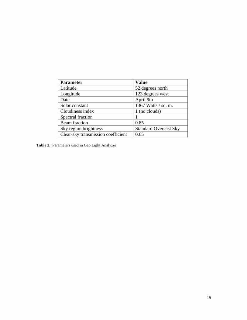
Parameter Value Latitude 52 degrees north Longitude 123 degrees west Date April 9th Solar constant 1367 Watts / sq. m. Cloudiness index 1 (no clouds) Spectral fraction 1 Beam fraction 0.85 Sky region brightness Standard Overcast Sky Clear-sky transmission coefficient 0.65

Table 2. Parameters used in Gap Light Analyzer

19

Figure 1. Locations of plot groups

20

Figure 2. Regions of the celestial hemisphere in which gap fractions were calculated. Zenith angles are in increments of 10 degrees and solar paths are shown in one-hour increments of local solar time.

21

Incoming Direct RadiationNo Clouds

0.0

0.5

1.0

1.5

2.0

2.5

3.0

3.5

4.0

4.5

6:00

7:00

8:00

9:00

10:0

0

11:0

0

12:0

0

13:0

0

14:0

0

15:0

0

16:0

0

17:0

0

MJ

/ sq

m /

hr

Figure 3. Hourly incoming direct radiation under clear skies on April 9th at 52 degrees north latitude

0

0.1

0.2

0.3

0.4

0.5

0.6

0.7

0.8

0.9

0 20 40 60 80 100

Zenith Angle

Diff

use

Rad

iatio

n, M

J / s

q.m

/ day

Figure 4. Above canopy diffuse radiation as a function of zenith angle

22

0.0

0.2

0.4

0.6

0.8

1.0

0.0 0.2 0.4 0.6 0.8 1.0

Rosita Method

Gap

Lig

ht A

naly

zer

Figure 5. Comparison of total radiation transmittances calculated for individual hemispherical photos by GLA and the Rosita method. Data are a subset of BOD1, BOD3, and BRC1.

23

Figure 6. Arrangement of fixed radius tree survey plots within a snow research plot using the 7.98 metre radius (200 square metre) plot as an example

Figure 7. Snow accumulation ratios versus canopy densities in all plots

24

Figure 8. Snow accumulation ratios vs. canopy density in each group

25

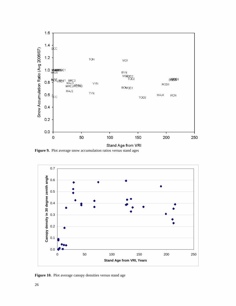
Figure 9. Plot average snow accumulation ratios versus stand ages

0.0

0.1

0.2

0.3

0.4

0.5

0.6

0.7

0 50 100 150 200 250

Stand Age from VRI, Years

Can

opy

dens

ity in

30

degr

ee z

enith

ang

le

Figure 10. Plot average canopy densities versus stand age

26

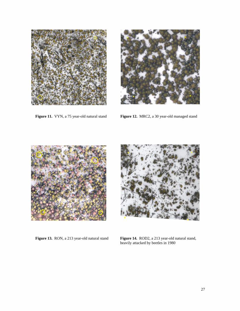
Figure 11. VYN, a 75 year-old natural stand Figure 12. MRC2, a 30 year-old managed stand

Figure 13. RON, a 213 year-old natural stand Figure 14. ROD2, a 213 year-old natural stand, heavily attacked by beetles in 1980

27

Figure 15a. Plot average radiation transmittance versus stand age from the VRI, except plot TON, which is estimated to be at least 130 years old. Circles indicate plots for which aerial photos are shown in Figures 11 - 14.

Figure 15b. Same data as Figure 12a, showing the data grouped into young managed stands, young natural stands, and old stands.

28

Figure 16b. Plot MO1 in April 2007

Figure 16a. Plot MO1 in April 2006

29

Figure 17. Plot average diffuse versus total radiation transmittances in all plots

Figure 18. Plot average sky view factors versus total radiation transmittances in all plots

30

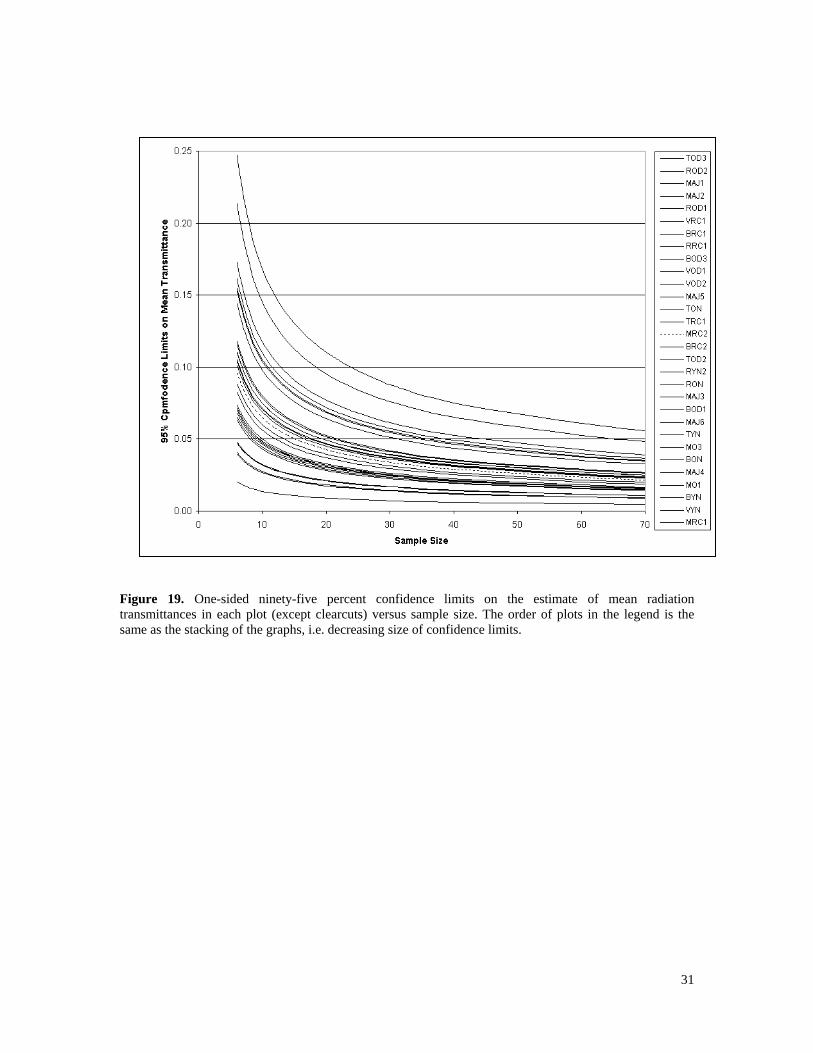
Figure 19. One-sided ninety-five percent confidence limits on the estimate of mean radiation transmittances in each plot (except clearcuts) versus sample size. The order of plots in the legend is the same as the stacking of the graphs, i.e. decreasing size of confidence limits.

31

Figure 20. Plot average radiation transmittances versus plot average Angular Canopy Gaps obtained from fisheye photos

32

Figure 21a. Plot average ablation rates in 2006 versus average radiation transmittances

33

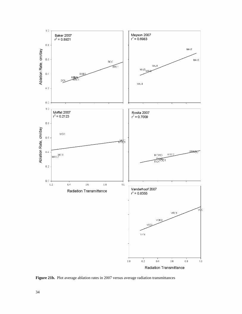
Figure 21b. Plot average ablation rates in 2007 versus average radiation transmittances

34