NCEE 2010–4002 U.S. DEpartmENt of EDUCatioN

Effects of Problem Based Economics on high school economics instruction Final Report

At WestEd

At WestEd

Effects of Problem Based Economics on high school economics instruction

Final Report

July 2010

Authors: Dr. Neal Finkelstein, Principal Investigator WestEd

Dr. Thomas Hanson WestEd

Dr. Chun-Wei Huang WestEd

Becca Hirschman WestEd

Min Huang WestEd

Project Officer: Ok-Choon Park Institute of Education Sciences

NCEE 2010-4002 U.S. Department of Education

U.S. Department of Education Arne Duncan Secretary Institute of Education Sciences John Q. Easton Director National Center for Education Evaluation and Regional Assistance Rebecca A. Maynard Commissioner July 2010 This report was prepared for the National Center for Education Evaluation and Regional Assistance, Institute of Education Sciences, under contract ED-06C0-0014 with Regional Educational Laboratory West administered by WestEd. IES evaluation reports present objective information on the conditions of implementation and impacts of the programs being evaluated. IES evaluation reports do not include conclusions or recommendations or views with regard to actions policymakers or practitioners should take in light of the findings in the report. This report is in the public domain. Authorization to reproduce it in whole or in part is granted. While permission to reprint this publication is not necessary, the citation should read: Finkelstein, N., Hanson, T., Huang, C.-W., Hirschman, B., and Huang, M. (2010). Effects of Problem Based Economics on high school economics instruction. (NCEE 2010-4002). Washington, DC: National Center for Education Evaluation and Regional Assistance, Institute of Education Sciences, U.S. Department of Education. This report is available on the Institute of Education Sciences website at http://ncee.ed.gov and the Regional Educational Laboratory Program website at http://edlabs.ed.gov. Alternate Formats Upon request, this report is available in alternate formats, such as Braille, large print, audiotape, or computer diskette. For more information, please contact the Department’s Alternate Format Center at 202-260-9895 or 202-205-8113.

ii

iii

Disclosure of potential conflict of interest The research team for this study was based at Regional Educational Laboratory West administered by WestEd. Neither the authors nor WestEd and its key staff have financial interests that could be affected by the findings of this study. No one on the 11-member Technical Working Group, convened annually by the research team to provide advice and guidance, has financial interests that could be affected by the study findings.*

* Contractors carrying out research and evaluation projects for IES frequently need to obtain expert advice and technical assistance from individuals and entities whose other professional work may not be entirely independent of or separable from the tasks they are carrying out for the IES contractor. Contractors endeavor not to put such individuals or entities in positions in which they could bias the analysis and reporting of results, and their potential conflicts of interest are disclosed.

Contents

Acknowledgments ........................................................................................................... vii

Executive summary........................................................................................................ viii

1. Introduction and study overview..................................................................................1Why study economics instruction? .................................................................................1 Typical economics instruction in high schools ...............................................................3 Problem-based economics instruction.............................................................................4 Conceptual framework ....................................................................................................7 Research domains and study questions ...........................................................................8 Roadmap of this report ....................................................................................................9

2. Study design and methodology ...................................................................................10Sample recruitment .......................................................................................................12 Random assignment ......................................................................................................14 Sample selection ...........................................................................................................16 Instruments ....................................................................................................................20 Data collection ..............................................................................................................29 Sample characteristics ...................................................................................................36 Data analysis methods...................................................................................................44

3. Implementation of the Problem Based Economics intervention .............................48Intervention description ................................................................................................48 Intervention implementation costs ................................................................................51

4. Impact results ...............................................................................................................52Overview.......................................................................................................................52 Student outcomes (primary) ..........................................................................................52 Teacher outcomes (secondary) ......................................................................................55 Sensitivity analyses .......................................................................................................56 Limitations of the analyses ...........................................................................................57

5. Summary of key findings.............................................................................................59Generalizability of the findings.....................................................................................59 Implications for future research ....................................................................................60

Appendix A. Study power estimates based on the final analytic samples .................61

Appendix B. Procedure for assigning new strata to the final analytic sample ..........63

Appendix C. Scoring procedures for the performance task assessments ...................66

iv

Appendix D. Sample test/survey administration guide ...............................................72

Appendix E. Teacher-level baseline equivalence tests..................................................75

Appendix F. Additional student-level baseline equivalence tests ................................78

Appendix G. Estimation methods...................................................................................83

Appendix H. Summary statistics of teacher data from teacher surveys.....................85

Appendix I. Sensitivity of impact estimates to alternative model specifications........87

Appendix J. Explanations for sample attrition .............................................................97

References.........................................................................................................................98

Figures

Figure 1.1. Logic model for the study of high school instruction with Problem Based Economics..............................................................................................7

Figure 2.1. Teacher Consolidated Standards of Reporting Trials (CONSORT) Diagram ..................................................................................................17

Figure 2.2. Consolidated Standards of Reporting Trials (CONSORT) Diagram of teachers providing student-level data ........................................................19

Figure 2.3. Student Consolidated Standards of Reporting Trials (CONSORT) diagram ...................................................................................................20

Figure 4.1. Intervention contrast on student Test of Economic Literacy, spring 2008 student cohort ...........................................................................................54

Figure 4.2. Intervention contrast on student performance task assessment, spring 2008 student cohort ............................................................................................54

Figure 4.3. Intervention contrast on teacher satisfaction with teaching materials and methods, spring 2008 semester...............................................................56

Tables

Table 2.1. Study characteristics and data collection schedule for high school instruction with Problem Based Economics ......................................................11

Table 2.2. Balanced incomplete block matrix sampling design for the performance tasks..........................................................................................................27

Table 2.3. Students taking each performance task booklet version, by experimental condition, spring 2008 semester..............................................................28

Table 2.4. Data collection activities...................................................................................30 Table 2.5. Response rates for each outcome measure .......................................................34 Table 2.6. School-level characteristics for randomized controlled sample .......................36 Table 2.7. School-level characteristics of 59 retained singleton schools, by

experimental condition..................................................................................................37 Table 2.8. School-level characteristics of 31 singleton schools that were

not retained, by experimental condition........................................................................38 Table 2.9. Number of teachers per school, by experimental condition .............................39

v

Table 2.10. Number of classes per teacher, by experimental condition ...........................40 Table 2.11. Teacher demographic information, by experimental condition......................40 Table 2.12. Key teacher measures at baseline, by experimental condition .......................41 Table 2.13. Student demographic information, by experimental condition ......................43 Table 2.14. Key student measures at baseline, by experimental condition .......................44 Table 4.1. Impact analysis of student outcome measures, spring 2008

student cohort ................................................................................................................53 Table 4.2. Impact analysis of teacher outcome measures, spring 2008

semester.........................................................................................................................55 Table A.1. Minimum detectable effect size for student outcome measures ......................61 Table A.2. Minimum detectable effect size for teacher outcome measures ......................62 Table B.1. Assigning two new strata to the final analytic sample.....................................64 Table C.1. Interrater analysis on performance task A .......................................................70 Table C.2. Interrater analysis on performance task B........................................................70 Table C.3. Interrater analysis on performance task C........................................................71 Table C.4. Interrater analysis on performance task D .......................................................71 Table C.5. Interrater analysis on performance task E........................................................71 Table E.1. Additional teacher measures at baseline, by experimental

condition........................................................................................................................75 Table E.2. Key teacher measures at baseline for 64 teachers who returned

student-level data, by experimental condition ..............................................................76 Table E.3. Additional teacher measures at baseline for 64 teachers who

returned student-level data, by experimental condition ................................................77 Table F.1. Additional student measures at baseline, by experimental

condition, categorical variables.....................................................................................79 Table F.2. Additional student measures at baseline, by experimental

condition, continuous variables.....................................................................................82 Table H.1. Summary of teacher data (continuous variables) from the

surveys, by data collection point and experimental condition ......................................85 Table H.2. Summary of teacher data (categorical variables) from the

surveys, by data collection point and experimental condition ......................................86 Table I.1. Sensitivity of impact estimates to alternative model

specification using various sample sets for student content knowledge in economics, spring 2008 student cohort.....................................................................88

Table I.2. Sensitivity of impact estimates to alternative model specification using various sample sets for student performance task assessment, spring 2008 student cohort ........................................................................90

Table I.3. Sensitivity of impact estimates to alternative model specification for teacher outcome measures .................................................................95

Table J.1. Explanation for sample attrition by assigned status ..........................................97

vi

Acknowledgments

The Regional Educational Laboratory (REL) West research team would like to acknowledge colleagues who made the study possible from the early design phases to the final analyses.

First, we thank the teachers, students, and their school-site colleagues who made every step of the program implementation and data collection possible. We recognize the burden associated with participating in a research study of this magnitude and thank them for their time, commitment, diligence, and interest over the past several years.

Colleagues at the Buck Institute of Education in Novato, California, the developers of Problem Based Economics, worked for several years with the research team as the study design was developed and the intervention was provided to teachers. We acknowledge the unwavering commitment of the implementation team and the entire staff that supported the project: Dr. John Mergendoller, Dr. Nan Maxwell (California State University, East Bay), Mr. John Larmer, Dr. Jason Ravitz, and Ms. Lois Gonzenbach.

The study was a collaboration of several research organizations that collected, archived, and scored the vast datasets assembled to support this study. We acknowledge the research teams at Empirical Education, Inc.; Educational Data Systems, Inc.; and the Sacramento County Office of Education, who provided invaluable support and precision in their work.

Finally, the REL West team would like to thank the Technical Working Group that provided guidance from the outset through to the final analyses: Dr. Jamal Abedi, University of California, Davis; Dr. Lloyd Bond, Carnegie Foundation for the Advancement of Teaching; Dr. Geoffrey Borman, University of Wisconsin; Dr. Brian Flay, Oregon State University; Dr. Tom Good, University of Arizona; Ms. Corinne Herlihy, Harvard University; Dr. Joan Herman, National Center for Research on Education, Standards, and Student Testing, University of California, Los Angeles; Dr. Heather Hill, Harvard University; Dr. Roger Levine, American Institutes for Research; Dr. Juliet Shaffer, University of California, Berkeley; and Dr. Jason Snipes, Academy for Educational Development.

vii

Executive summary

For decades, economists, prominent educators, Nobel laureates, and business and government leaders have advocated for economic literacy as an essential component in school curricula. Their arguments have ranged from the need to improve people’s ability to manage personal finances to the value of economic education for critical thinking and an informed citizenry. To cite one example, Nobel laureate and Yale economist James Tobin argued in a July 9, 1986, Wall Street Journal column: “The case for economic literacy is obvious. High school graduates will be making economic choices all their lives, as breadwinners and consumers, and as citizens and voters. A wide range of people will be bombarded with economic information and misinformation for their entire lives. They will need some capacity for critical judgment. They will need it whether or not they go to college” (Tobin as quoted in Walstad 2007).

At the federal and state levels, economics has received increasing attention as a critical content area for K–12 education. In 1994 the Goals 2000 Educate America Act identified economics as one of nine core subject areas for developing content standards. Three years later, the National Council on Economic Education (NCEE) led a coalition of organizations (including the National Association of Economic Educators, the Foundation for Teaching Economics, and the American Economics Association’s Committee on Economic Education) to develop voluntary content standards to guide instruction. The standards describe the economics content for grades 1–12 and include 211 benchmarks detailing what students should know and be able to do (Siegfried and Meszaros 1998). According to the most recent NCEE survey of 2007, 48 states now include content standards in economics, with 40 requiring implementation of the standards, 23 requiring testing, and 17 requiring an economics course for graduation (NCEE 2007).

The NCEE standards were subsequently revised in developing the 2006 National Assessment of Educational Progress (NAEP) in Economics, the first federal testing of high school students in this content area. A 2007 NAEP report on results of the assessment, given to a nationally representative sample of 11,500 grade 12 students in 590 public and private schools, found that 42 percent of 12th graders reached the proficient level and that 79 percent scored at or above the basic achievement level (National Assessment of Educational Progress 2007).

While there is growing agreement on the need for some economics content in K–12 education, there is less agreement about where it fits into the curriculum, effective ways of teaching it, and how much subject-area background should be required of classroom instructors (Watts 2006). Watts (2006) reports that in states where economics is required for high school graduation, it is typically taught by following the state-adopted content standards, which are supported by a textbook. The format is generally one in which teachers provide direct instruction through a lecture format and encourage student discussion (see, for example, Mergendoller, Maxwell, and Bellisimo 2000). The teachers’ objective is to follow the text from beginning to end, covering concepts of theoretical and applied micro- and macroeconomics. In practice, there is variation from classroom to classroom (Walstad 2001). Teachers not only vary the sequencing of the course, but also add content through lessons and activities to augment the textbook (Schug, Dieterle, and Clark 2009). The variation is largely due to the fact that teachers and their districts remain ultimately responsible for designing the curriculum (Walstad 2001).

viii

In contrast with the typical, textbook-driven curriculum for high school economics, another method uses a problem-based approach. Teachers use a specific economic problem as the basis for a set of disciplined and strategic analytic steps. Students learn to contextualize, understand, reason, and solve what may, at the outset, have been a problem for which they had no analytic tools. It is an inquiry-based pedagogy rooted in the constructivist ideas and developmental learning theories of John Dewey and Jean Piaget (Memory et al. 2004), which have been applied in diverse educational domains.

The University of Delaware’s Center for Teaching Effectiveness defines problem-based learning in all subject domains as an “instructional method characterized by the use of ‘real-world’ problems as a context for students to learn critical thinking and problem-solving skills” (Duch 1995, paragraph 1). Broad interest in the application of problem-based instruction is evident in several studies (Bridges 1992; Achilles and Hoover 1996; Artino 2008). Advocates argue that, “unlike traditional lecture-based instruction, where information is passively transferred from instructor to student, problem-based learning (PBL) students are active participants in their own learning” (Massa 2008, p. 19).

A problem-based approach is frequently a defined component of current high school reform models (Expeditionary Learning Outward Bound 1999; Honey and Henríquez 1996; Newmann and Wehlage 1995); however, teachers and schools often have difficulty incorporating problem-based teaching into classroom instruction (Hendrie 2003). One approach has been developed by the Buck Institute for Education.

Since 1995, the Buck Institute has partnered with university economists and expert teachers to create the Problem Based Economics curriculum. The curriculum was developed to respond to NCEE standards, and it is supported by professional development for teachers.

This study examines whether the Problem Based Economics curriculum developed by the Buck Institute for Education improves grade 12 students’ content knowledge as measured by the Test of Economic Literacy, a test refined by NCEE over decades. Students’ problem-solving skills in economics were also examined using a performance task assessment. In addition to the primary focus on student achievement outcomes, the study examined changes in teachers’ content knowledge in economics and their pedagogical practices, as well as their satisfaction with the curriculum.

The professional development intervention consisted of a 40-hour economics course for teachers, held over five days in summer 2007. Participating teachers also received additional support as they used the curriculum through a series of five scheduled phone conferences with fellow participating teachers. This allowed teachers to discuss curriculum pacing and work together to develop solutions to challenges encountered in the classroom. Participating teachers agreed to teach core concepts in economics, as identified by national economics standards, using the curricular materials provided.

The study was designed as an experimental trial. It was implemented from summer 2007 through spring 2008 in high schools in Arizona and California. For both of these states, high school economics has become a required course for graduation and relevant to schools and districts as a result. Arizona targeted the graduating class of 2009 as the first cohort of high school students that was required to complete a course in economics; California has had this requirement in place

ix

since 2005. Study participants included 128 economics teachers from 106 schools. Teachers were randomly assigned to the intervention or control condition (64 teachers each). Twenty-two intervention teachers and 23 control teachers dropped out of the study following random assignment. Because attrition after random assignment is a potential threat to the integrity of the experimental design, extensive analyses were conducted to document differences in attrition rates, reasons for attrition, and baseline characteristics of the retained sample (see sections on “sample selection” and “sample characteristics” in Chapter 2 as well as Appendixes E, F, and J). These analyses suggest that teacher attrition after random assignment was unlikely to bias estimation of program impacts. Since the teacher level data for those teachers who dropped out of the study was not available to the study team, it was not feasible to examine how the teacher sample characteristics changed due to attrition. Data were subsequently collected from the remaining 83 teachers. The final analytic sample used for examining the primary research questions included 4,350 students from 64 teachers (2,502 students from 35 intervention teachers and 1,848 students from 29 control teachers). Eighty-eight percent of students with valid posttest measures were enrolled in grade 12; the remaining 12 percent were in grade 11. Attrition and missing outcome data did not significantly affect the study’s statistical power to detect the intervention contrast that is fully discussed in Chapter 2.

The research questions asked whether Problem Based Economics changes:

• Students’ content knowledge in economics.

• Students’ problem-solving skills in economics.

• Teachers’ content knowledge in economics.

• Teachers’ instructional practices.

• Teachers’ satisfaction with teaching materials and methods used to teach economics.

The analyses for this study compare outcomes for students and teachers in the intervention group with their counterparts in the control group after the economics course has been completed. The analyses involve fitting conditional multilevel regression models (HLM), with additional terms to account for the nesting of individuals within higher units of aggregation (e.g., see Goldstein, 1987; Raudenbush & Bryk, 2002; Murray, 1998). The design thus involves clustering at the classroom level, as students are nested within teachers.

The test of whether gains in economic literacy are seen between intervention and control students was accomplished by the administration of the Test of Economic Literacy (TEL),a 40-item closed-response economics exam (Walstad and Rebeck, 2001). The research team augmented this outcome measure with an opportunity to test students’ abilities to reason with the concepts they had learned. Each TEL item was rated “correct” (1 point) or “incorrect” (0 points); the possible overall TEL score ranged from 0 to 40. A set of “performance tasks”, developed by the University of California, Los Angeles’s National Center for Research on Education, Standards, and Student Testing (UCLA CRESST), gave students the ability to demonstrate problem-solving skills as they answered open-ended essay questions. The five assessment tasks used in this study focused on monetary policy/federal funds, monetary policy/employment, fiscal policy, consumer demand, and opportunity costs. Each student was randomly assigned two tasks.

Both the TEL posttest and the performance task assessments were administered to the students by designated proctors (such as student counselors) at the end of the spring semester.

x

Performance task assessment scoring was done by Educational Data Systems, Inc., with support from the Sacramento County Office of Education. Because each task was evaluated on a three-point scale (1–3) by two raters, the possible score range for each task was from 2 to 6, which translates into a range of 4 to 12 for the composite score for each student. The resulting composite scores were then analyzed. Overall, the test of the curriculum was whether students, working with well-trained and supported teachers, demonstrated a level of economic performance above that of students who took traditional economics courses.

The same TEL was also administered to the participating teachers to assess their content knowledge in economics. In addition, two measures were also collected through teacher surveys. The “pedagogical practices used” scale consisted of nine items, each rated on a five-point scale. Teachers were asked to indicate how often they had assigned various types of assignments to their students. The scale scores were calculated by summing nine items, and therefore the score ranged from 9 to 45. The “satisfaction with teaching materials and methods” scale consisted of two items, each rated on a five-point scale where 1 was “very unsatisfied” and 5 was “very satisfied.” Teachers were asked to assess their satisfaction with the curriculum materials and methods used to teach economics. The scale scores were calculated by summing two items, and therefore the score ranged from 2 to 10.

The counterfactual for the study was the typical instruction in high school economics classrooms. Teachers in control schools participated in their regular annual professional development activities during the 2007/08 academic year and continued their usual instructional practices in economics classrooms.

The analysis at the primary (student) level supports the following:

• A statistically significant finding that students whose teachers had received professional development and support in Problem Based Economics (model-adjusted mean score = 22.61) outscored their control group peers (model-adjusted mean score = 20.01) on the TEL by an average of 2.6 test items (effect size = 0.32).

• The outcomes on student measures of problem-solving skills and application to real-world economic dilemmas also showed significant differences in favor of the intervention group (model-adjusted mean score for the intervention group was 6.72 versus 6.18 for the control group; the difference of 0.54 corresponded to an effect size of 0.27).

The study also confirmed the following at the secondary (teacher) level:

• No statistically significant difference between the intervention and control groups on teachers’ knowledge of economics (model-adjusted means were 37.15 and 36.86 for the intervention and control group teachers, respectively). As discussed in the conclusions of the report, a ceiling effect on the Test of Economic Literacy instrument may have masked any true content gains for teachers.

• No statistically significant difference in teachers’ pedagogical style with the survey measures used (model-adjusted means were 29.92 and 26.60 for the intervention and control group teachers, respectively).

• Statistically significant differences in favor of the intervention group teachers on a measure of satisfaction with the teaching materials and methods (model-adjusted means were 8.35 and

xi

6.88 for the intervention and control group teachers, respectively; the difference of 1.47 corresponded to an effect size of 1.09).

Since this study recruited a purposively targeted sample, these findings should only be generalized to teachers and schools where the economics program and the associated professional development are a priority. This holds for the original recruited 128 teachers who agreed to participate before data collection, for the remaining 83 teachers after the initial attrition, and for the final 64 teachers who provided student level data. From the perspective of the students, since their participation in the study was voluntary (as was the case for the participating teachers), we cannot quantify whether students unwilling to participate in the economics tests would have performed differently than the study sample described in this report.

To examine the robustness of these primary findings, additional models were estimated with different combinations of baseline covariates for different analytic samples. The results indicate that the impact estimates do vary when different combinations of covariates are included in the models. Specifically, the differences in point estimates between models that were tested are largely due to intervention-control differences on the teacher baseline TEL measure. Although the impact estimates on TEL scores varied, effect sizes ranged from 0.17 to 0.42 across all the models estimated to assess the sensitivity of results. The sensitivity tests therefore are consistent with the key study finding that students in PBE classrooms outperformed their counterparts in control classrooms. The detailed findings from these sensitivity analyses are presented in Appendix I.

Replication of this experiment is necessary to refine understanding of the impacts associated with the curriculum and the professional development model. Of particular note is that the intervention teachers had a higher level of satisfaction with the Problem Based Economics curriculum materials and methods than did the control teachers who used “ordinary” economics teaching materials and methods. At the same time, no significant differences in pedagogical practice were detected. Additional investigation on measurement in this area is warranted. The survey items used in this study may not have been sufficiently refined to pick up nuances in pedagogical approaches on self-reported data collection.

Future study of this curriculum might emphasize the classroom observation component to get a clearer understanding of teachers’ pedagogical strategies in varying classroom settings. From observations in intervention and control classrooms, it did not appear to the research team that having and using the problem-based learning curriculum automatically enforced a more hands-on, exploratory classroom learning style. Additional study in this area might help to refine the pedagogical strategies and allow for additional support and practice for teachers on implementing the curriculum effectively.

xii

1. Introduction and study overview

The primary purpose of this study is to assess student-level impacts of a problem-based instructional approach to high school economics. The study was designed as a within-school randomized controlled trial. Economics is a required course for high school graduation in California and, as of the 2008/09 school year, Arizona, the two study states.

The curriculum approach examined here was designed to increase class participation and content knowledge for high school students who are learning economics. This study tests the effectiveness of Problem Based Economics, developed by the Buck Institute for Education, on student learning of economics content and problem-solving skills. Student achievement outcomes are of primary importance and are hypothesized to be mediated by changes in teacher knowledge and pedagogical practice. This study targeted high schools in both urban and rural areas and engaged teachers who committed to teach economics during the 2007/08 academic year.

Why study economics instruction?

Economists, prominent educators, and business and government leaders have advocated for developing economic literacy as an essential component in school curricula. Their arguments have ranged from the need for improving the ability to manage personal finances to the value of economic education for critical thinking and an informed citizenry (Stigler, 1970; Bernanke 2006; Walstad 2007).

Many proponents, including Nobel laureates in economics and the chairman of the Federal Reserve, have framed the case for economic literacy in terms of citizenship. For example, in a 1970 Journal of Economic Education article, Nobelist George Stigler (1970, p. 82) wrote: “The public has chosen to speak and vote on economic problems, so the only open question is how intelligently it speaks and votes.” In a July 9, 1986, Wall Street Journal column, Nobel laureate and Yale economist James Tobin argued: “The case for economic literacy is obvious. High school graduates will be making economic choices all their lives, as breadwinners and consumers, and as citizens and voters. A wide range of people will be bombarded with economic information and misinformation for their entire lives. They will need some capacity for critical judgment. They will need it whether or not they go to college” (Tobin as quoted in Walstad 2007). And at a May 23, 2006, U.S. Senate hearing, Federal Reserve Chairman Ben Bernanke testified that “the Federal Reserve System has long recognized the value of financial and economic literacy for producing better-informed citizens and consumers.” He cited findings from the Jump$tart Coalition for Personal Financial Literacy, which has tested high school students annually on their financial literacy since 1997. Student performance, he noted, “has not improved during that time,” and the results “also show a gap in financial literacy between minority and non-minority students” (Bernanke 2006, paragraph 23).

Economics has received increasing attention as a critical content area for K–12 education. A nonprofit advocacy group, the Council for Economic Education (CEE, formerly the National Council on Economic Education), the recipient of federal grants under the Excellence in

1

Economic Education Act of 2004, has played a significant role in supporting and publishing research on the status of K–12 economics instruction and in promoting effective economics curricula.1 Its president, Robert F. Duvall, described the problem of current instructional approaches in testimony in April 2009 before the U.S. Senate Subcommittee on Oversight of Government Management, the Federal Workforce, and the District of Columbia:

Are our teachers preparing students for the economy of the future? It is often said that today’s education curriculum is rooted in yesterday’s economy, and that a rapidly changing and technologically driven marketplace requires new educational approaches. The skill-set today’s young people will need to possess in order to succeed as adults is likely to be markedly different than that of a generation ago. This skill-set must empower students with an economic and entrepreneurial way of thinking, to be prepared for the myriad opportunities— and threats—they will encounter as adults. The degree to which they succeed in this endeavor will shape not only their futures and fortunes, but the level of competitiveness and dynamism of the American economy. (Duvall 2009, p. 2)

In 1994 the Goals 2000 Educate America Act identified economics as one of nine core subject areas for developing content standards. Three years later, the National Council on Economic Education (NCEE) led a coalition of organizations (including the National Association of Economic Educators, the Foundation for Teaching Economics, and the American Economics Association’s Committee on Economic Education) to develop voluntary content standards for instruction in schools (National Council on Economic Education 1997). Its 20 content standards describe “what economics should be taught in grades 1–12 (Siegfried and Meszaros 1998). [They] are divided into 211 ‘benchmarks’ that describe what a student should be able to do with that understanding at grades 4, 8, and 12” (Walstad 2007, paragraph 14).

The NCEE standards were subsequently revised to develop the 2006 National Assessment of Educational Progress (NAEP) in Economics, the first federal testing of high school students in this content area. A report detailing results of the assessment, given to a nationally representative sample of 11,500 grade 12 students in 590 public and private schools, found that 42 percent of 12th graders reached the proficient level and that 79 percent scored at or above the basic achievement level (National Assessment of Educational Progress 2007). In a statement accompanying the report, Darvin Winick, chairman of the National Assessment Governing Board, wrote, “I have too often been surprised and disappointed in high school graduates’ (and for that matter college graduates’) lack of understanding of important concepts; for example, compound interest, the cost of credit, and, in general, the future value of money.” Citing findings from a study of family housing decisions, he added that “most homeowners did not know how much they borrowed to buy their house, how much they owed, or at what interest rate they agreed to repay the borrowing. When I mentioned this finding to a group of bank officers, they were surprised that I was surprised” (Winick 2007, p. 2).

In general, high school economics does not help students understand our economic system, the relationships between supply and demand and consumers and producers, and the workings of world trade (National Council on Economic Education 1999). Most teachers are not adequately

1 Founded in 1948, the Council for Economic Education is a nonprofit advocate and service provider promoting economics, personal finance, and entrepreneurship education in the nation’s schools. Since 1998 it has published five national survey reports on the status of economics teaching in all states.

2

prepared to teach economics because of poor content knowledge, a large gap in professional development, and a lack of accessible and relevant teaching materials (Walstad 2007). Identifying a reliable and effective response to this problem could have great value nationally.

Federal support for improving the quality of economics education has come through grants administered since 2004 by the U.S. Department of Education under the Excellence in Economic Education Act (20 USC 7267), as part of the No Child Left Behind Act of 2001. Through this competitive grant process, the Excellence in Economic Education (EEE) program “promote[s] economic and financial literacy among all students in kindergarten through grade 12 by awarding a competitive grant to a national nonprofit educational organization that has as its primary purpose the improvement of the quality of student understanding of personal finance and economics” (U.S. Department of Education 2001).

The National Council on Economic Education (recently renamed the Council for Economic Education) is the only organization reported to have been awarded EEE grants. (U.S. Department of Education 2010). Through this organizations work, a variety of efforts have been launched to support teacher training, curriculum materials disbursement, research involving measuring student learning, student and school-based activities, and best practices. The program also serves to advance student understanding of personal finance and economics and to:

• Increase students’ knowledge of and achievements in economics.

• Strengthen teachers’ understanding of and competence in economics.

• Encourage economic research and development.

• Assist states in measuring the impact of education in economics.

• Leverage and expand increased private and public support for economic education partnerships at the national, state, and local levels. (U.S. Department of Education 2001)

According to the most recent NCEE survey of 2007, 48 states now include content standards in economics, with 40 requiring implementation of the standards, 23 requiring testing, and 17 requiring a course in the subject for graduation (National Council on Economic Education 2007).2 As of 2005, states requiring a high school economics course included Alabama, California, Florida, Idaho, Indiana, Michigan, New York, and Texas. Arizona joined the list in 2006, with an expectation that the graduating high school class of 2009 would have met the new course requirement. Beyond these state trends, many districts, including those in large urban areas, have economics standards in their curricula, offer elective or required courses in economics, and test student learning in the subject (Watts 2006).

Typical economics instruction in high schools

Even with the recent national attention on economics literacy in K–12 education (e.g. NAEP economics test in 2006; EEE grant program in 2004 and 2005), there is less agreement about

2 Since 1998, the NCEE has conducted five national surveys, with state-by-state snapshots detailing what states are doing with standards, implementation, testing, and graduation requirements in economics.

3

where economics fits into the curriculum, effective ways of teaching it, and how much subject-area background should be required of classroom instructors (Watts 2006).

Watts (2006) reports that in states where economics is required for high school graduation, it is typically taught by following the state-adopted content standards, which are supported by a textbook. The format is generally one in which teachers provide direct instruction through a lecture format and encourage student discussion (see, for example, Mergendoller, Maxwell, and Bellisimo 2000). The teachers’ objective is to follow the text from beginning to end, covering concepts of theoretical and applied micro- and macroeconomics. In practice, there is variation from classroom to classroom (Walstad 2001). Teachers not only vary the sequencing of the course, but also add content through lessons and activities to augment the textbook (Schug, Dieterle, and Clark 2009). The variation is largely due to the fact that teachers and their districts remain ultimately responsible for designing the curriculum (Walstad 2001).

To add new content areas, an individual teacher generally provides supplemental instructional materials. These may include current events articles passed out in class or homework assignments that rely on a web site for independent study (Schug, Dieterle, and Clark 2009). The Stock Market Game, a popular augmentation in recent years, brings a simulated stock market into the classroom for several days or weeks (Schug, Dieterle, and Clark 2009; Lopus and Placone 2002). In general, decisions to use supplemental materials are made by individual teachers, although some school districts mandate systemwide requirements that are applied across all schools (Walstad 2001).

Problem-based economics instruction

In contrast with the textbook-driven curriculum for high school economics, another method uses a problem-based approach. Teachers use economic problems and follow a set of disciplined and strategic analytic steps. The intent is that students learn to contextualize, understand, reason, and solve what may at the outset have been a problem for which they had no analytic tools. It is an inquiry-based pedagogy rooted in the constructivist ideas and developmental learning theories of John Dewey and Jean Piaget (Memory et al. 2004), which have been applied in diverse educational domains. In the early 1970s, a problem-based approach was pioneered in teaching medicine at McMaster University and in the work of Howard Barrows at the University of Southern Illinois Medical School (Bridges 1992).

The University of Delaware’s Center for Teaching Effectiveness defines problem-based learning in all subject domains as an “instructional method characterized by the use of ‘real-world’ problems as a context for students to learn critical thinking and problem-solving skills” (Duch 1995, paragraph 1). Broad interest in the application of problem-based instruction is evident in several studies (Bridges 1992; Achilles and Hoover 1996; Artino 2008). Advocates argue that, “unlike traditional lecture-based instruction, where information is passively transferred from instructor to student, problem-based learning (PBL) students are active participants in their own learning” (Massa 2008, p. 19).

In the literature on problem-based learning, there is a gap between the theory and the guidelines for what constitutes effective problem construction (Gijselaers 1996). There is also debate over the optimal degree of guided instruction in effective problem- and inquiry-based learning (Kirschner, Sweller, and Clark 2006; Hmelo-Silver, Duncan, and Chinn 2007).

4

A problem-based approach is frequently a defined component of current high school reform models (Expeditionary Learning Outward Bound 1999; Honey and Henríquez 1996; Newmann and Wehlage 1995); however, teachers and schools often have difficulty incorporating problem-based teaching into classroom instruction (Hendrie 2003). One approach has been developed by the Buck Institute for Education.

Since 1995, the Buck Institute has partnered with university economists and expert teachers to create the Problem Based Economics curriculum. The curriculum was developed to respond to NCEE standards, and it is supported by professional development for teachers. The Buck Institute has partnered with the Centers for Economic Education, affiliated with NCEE, to disseminate the materials.

In the curriculum described in this report and tested in this research study, the problem-based pedagogical approach was designed around a particular curriculum that lends itself to the strategy. Each curriculum module is set up around a case study that is well-suited to student-driven problem solving and a staggered learning and reinforcement of core concepts and analytic approaches. Units lasting 4–15 instructional days provide clear instructions for covering core content. The curriculum is introduced to teachers during a five-day professional development workshop led by expert teachers who have used the materials extensively in classrooms. In a Problem Based Economics classroom where implementation is consistent with the curricular design, an observer might see the following:

• Students confronting a real-world dilemma that allows for more than one possible solution through analysis, investigation, research, and discussion.

• Students seeking knowledge needed to understand and solve the problem.

• Students intrigued by the problem they are addressing and motivated to learn the standards-based content.

Each module has at least two components: a teaching guide and collateral materials for students, and, when applicable, a DVD with video clips that support the topic. The teaching guide is the cornerstone of each module. It lays out for teachers the problem statement, introduction, placement in curriculum, concepts taught, objectives, content standards, time required, lesson description, resource materials, sequence of the unit, procedures, and do’s and don’ts. The collateral materials for students play a key role as well. Some of the materials are worksheets that allow students to practice basic analytic skills relevant to the module; the worksheets are provided by the teacher at critical instructional points. Other materials provide sequenced information that allows students to build the case over days of study. For example, halfway through a unit, the teacher might provide a memo documenting a stakeholder’s position on a critical component of the case. Students must then assimilate and resolve the new information or perspectives.

The following description of the problem-based approach illustrates how it differs from the typical direct instruction approach found in most economics classrooms:

These units, which can take from one day to three weeks to complete, scaffold and, to some degree, constrain teacher and student behavior. Each unit contains seven interrelated phases: entry, problem framing, knowledge inventory, problem research and resources, problem twist, problem log, problem exit, and problem debriefing. Student groups generally move through the phases in the order indicated, but may return to a

5

previous phase or linger for a while in a phase as they consider a particularly difficult part of the problem. The teacher takes a facilitative role, answering questions, moving groups along, monitoring positive and negative behavior, and watching for opportunities to direct students to specific resources or to provide clarifying explanations. In this version of problem-based learning, students do not learn entirely on their own; teachers still “teach,” but the timing and the extent of their instructional interventions differ from those used in traditional approaches. Problem-based learning teachers wait for teachable moments before intervening or providing needed content explanations, such as when students want to understand specific content or recognize that they must learn something. (Mergendoller, Maxwell, and Bellisimo, 2006, p. 1)

Three nonexperimental studies (Ravitz and Mergendoller 2005; Maxwell, Mergendoller, and Bellisimo 2005; Moeller 2005) have concluded that the Buck Institute for Education’s Problem Based Economics curriculum and its related pedagogical practices appear to benefit low-performing students (Mo and Choi 2003; Maxwell, Mergendoller, and Bellisimo 2005; Ravitz and Mergendoller 2005; Moeller 2005).

The first study, using a descriptive pre-post design, examined the factors that shape implementation of problem-based instruction and their relationship to student learning. The study included 15 teachers and 1,162 students and collected data through student and teacher background surveys, student and teacher checklists of practices used and their helpfulness, and pre-, post-, and final (delayed post-) content tests (Ravitz and Mergendoller 2005). The study related the background characteristics of the teachers and students to learning outcomes and explored whether specific instructional practices were related to learning gains in economics.

The teacher participants were chosen as a convenience sample and participated in a short professional development training covering two Problem Based Economics units: “The High School Food Court” (microeconomics) and “The President’s Dilemma” (macroeconomics). Teachers incorporated these units into their regular classrooms. The study did not include a comparison group. Student’s prior achievement patterns were by proxy, measured by surveying students about the grade they believed they would earn in the economics course coupled with their overall college aspirations. For example, students who had low expectations for their course grade and low levels of college ambition were categorized as having low prior achievement. Learning outcomes were measured by tests constructed by the curriculum developer. They included tests at the beginning and end of each curriculum unit, and a final exam at the end of the semester. The largest gains were among students who had reported low levels of prior achievement (reported effect size of 0.5).Researchers also found negative correlations between the use of the PBE problem logs—a featured pedagogical strategy used to support the curriculum—and student learning gains. Since implementation varied by teacher and there was no comparison group, the authors suggested further study to systematically examine how implementation practices affect student learning.

In the second study, researchers examined whether problem-based learning enhanced student and teacher knowledge and learning of macroeconomics. Data were collected from 252 economics students and five teachers in five high schools. The Problem Based Economics approach is reported to have increased learning of macroeconomics, especially when instructors were well trained (Maxwell, Mergendoller, and Bellisimo 2005). The five participating teachers received training in Problem Based Economics; data were captured during the fall semester of 1998. Teachers taught at least two economics courses during the semester, with one course following

6

7

the Problem Based Economics curriculum (“The President’s Dilemma”) and the other taught in a more traditional lecture-oriented format. The teacher chose which class would receive Problem Based Economics instruction. A 16-item pre- and posttest was used to assess student achievement gains. At the conclusion of the study, the Problem Based Economics students were found to outperform the students who had not received the PBE curriculum (reported effect size of 0.54).

Because this study found implementation to vary in part with teacher experience, a third study (Moeller 2005) examined the factors that influence implementation of the Problem Based Economics curriculum. The study found that teachers who taught in schools that did not use problem based instruction had a more difficult time implementing the PBE curriculum than teachers in schools where the approach was common.

The results of these three research studies have been used formatively to improve the professional development approaches the Buck Institute uses so that it can better support teachers in integrating problem-based learning into their economics curriculum.

Building on this earlier work, the study detailed in this report examines student and teacher impacts in a randomized controlled trial to measure summative effects. Specifically, this large-scale trial tests research hypotheses at the student and teacher levels to test for causal relationships. The implementation approach provides not only base instruction through the summer professional development program, but also ongoing support during the next two semesters. The earlier studies reported limitations in their design, sample size, and measurement components. In this study, the combination of the randomized controlled trial design, sufficient statistical power to detect small effects, and series of reliable and valid measures brings forth additional information on the effectiveness of the Problem Based Economics curriculum.

Conceptual framework

The study is predicated on the following logic model (figure 1.1). Student performance gains in economics are mediated by changes in teacher knowledge and in teacher practice in the classroom. Figure 1.1. Logic model for the study of high school instruction with Problem Based Economics

Source: Authors’ construction.

As explained in chapter 3, the logic model begins with an extensive review of the Problem Based Economics curriculum for economics teachers in the context of problem-based pedagogical strategies. Over five days, with additional support throughout the school year, economics teachers have the opportunity to learn and review fundamental concepts in economics as they rehearse the delivery of curriculum modules provided by the developer. Delivery of the curriculum modules is modeled by master teachers with years of experience delivering the curriculum, thus melding content and pedagogical practice. The teachers receiving professional development assume the role of students for considerable portions of the five-day training to appreciate the distinctive approaches of problem-based instruction.

The logic model posits that this teacher professional development translates into changes in pedagogical teacher practice as the curriculum is delivered to students. Problem-based instruction is intended to engage students in a set of student-driven investigations of the analytic challenges presented by the complex case studies at the center of the curriculum. For example, in the curriculum module “The President’s Dilemma,” students working in groups over several weeks wrestle with federal budget deficits and the competing views and perspectives of policymakers, taxpayers, corporations, and lobbyists while learning about the economics of government borrowing, economic stimulus, and the challenges of inflation. Classroom activities, classroom management, and the balance between student-led and teacher-led instruction are intended to reinforce the pedagogical strategies provided to teachers during professional development.

Finally, the third stage in the logic model captures student performance by focusing on economic concepts and problem-solving skills. The curriculum has been designed to embed key concepts in economics that are consistent with state standards in economics and are supported by the nation’s largest economics education professional organization, CEE/NCEE. The test of the curriculum is whether intervention students, working with well-trained and supported teachers, demonstrate a level of economic performance above that of students who take traditional economics courses.

Research domains and study questions

Based on this logic model, the study is guided by a set of research questions, and underlying domains that reflect outcome measures for students and teachers. Specifically, one set of domains represents various aspects of student performance as indicated in the conceptual framework; another set of domains is used to represent various intervention impacts on teachers. The study was designed to examine whether there were any intervention impacts on student performance (primary outcomes) and/or whether there were any intervention impacts on teachers (secondary outcomes).

Formally stated, impacts on students are considered the confirmatory primary (P) outcomes in this study:

• Domain P1: content knowledge assessed by Test of Economic Literacy.

• Domain P2: problem-solving skills measured by the composite score on open-ended response performance assessments.

8

Research hypothesis I: Problem Based Economics has a positive or negative impact on students in either domain P1 or domain P2.

Similarly, impacts on teachers are treated as secondary (S) outcomes:

• Domain S1: content knowledge assessed by Test of Economic Literacy.

• Domain S2: pedagogical practices measured by a teacher survey.

• Domain S3: attitudinal changes measured by a teacher survey.

Research hypothesis II: Problem Based Economics has a positive or negative impact on teachers in domain S1 or domain S2 or domain S3.

Consistent with these research domains, the five research questions are as follows:

1. Does PBE change students’ content knowledge in economics?

2. Does PBE change students’ problem-solving skills in economics?

3. Does PBE change teachers’ content knowledge of economics?

4. Does use of PBE change economics teachers’ instructional practices?

5. Does the use of PBE change the satisfaction with teaching materials and methods used to teach economics?

The analysis is designed to formally test the Research hypotheses, stated above, at the student and teacher level, respectively. The intervention would be found to have a positive impact on student gains if either research question 1 or 2 demonstrated a statistically significant positive treatment effect. The intervention would be found to have a positive impact on teachers if either research question 3 or 4 or 5 demonstrated a statistically significant positive treatment effect.

Roadmap of this report

Chapter 2 describes the study design in detail, including sample recruitment (teachers and students), random assignment, data collection, final study sample, and data analysis methods. Chapter 2 also examines sample attrition and details baseline equivalence at both teacher and student levels. Chapter 3 describes the intervention. Chapter 4 reports the impact analyses for the experimental findings consistent with the established research domains and questions. Finally, chapter 5 summarizes the key findings and explores what the results might mean to educators, policymakers, and researchers.

9

2. Study design and methodology

The evaluation of the Problem Based Economics curriculum used an experimental design that randomly assigned teachers to an intervention or control group. Teachers in the intervention group participated in a five-day training session during the summer before implementing the curriculum in their economics instruction.3 The teachers received the curriculum materials at the start of the training session for use during the professional development program and for subsequent classroom instruction. Control teachers participated in their regular professional development activities and continued their usual instructional practices in economics classrooms during the 2007/08 academic year. As a courtesy, following all data collection activities for the study, control group teachers were offered the chance to receive professional development in Problem Based Economics.

Teachers were the unit of randomization. Students, the primary subjects of this study, were nested within teachers. Teachers were randomly assigned to the intervention or control condition and remained in the assigned condition until the end of the study. (Key design features are shown in table 2.1.)

High school economics is taught as a one-semester course – a fact that played into the design of the experiment and subsequent measurement details. Because of the pedagogical changes required to ensure complete implementation of the intervention, the study was conducted over one summer (2007) and two consecutive academic semesters (fall 2007 and spring 2008). Teachers had the opportunity to teach students with the new instructional approach for two semesters while receiving additional support from the curriculum developer and master teachers in economics. As a requirement for study participation, teachers were expected to teach consecutive semesters of economics during the academic year. This sequencing allowed intervention teachers to become better acquainted with the new instructional approach and the five curricular modules before the spring 2008 semester. Two cohorts of students were exposed to participating teachers—one cohort in the fall semester and a second cohort in the spring semester.

The teachers’ measurement timeline covered an entire academic year, while student exposure to the intervention was over a single semester in spring 2008. Students who enrolled in a single-semester high school economics class in spring 2008 received either the Problem Based Economics curriculum or the typical course. This study, therefore, examines outcomes associated with the spring 2008 semester for students who took economics.

3 Economics teachers assigned to the intervention condition were not expected to use the curriculum in classes designed for special education students or students with substantially limited English proficiency.

10

Table 2.1. Study characteristics and data collection schedule for high school instruction with Problem Based Economics

Study design Cluster-randomized trial

Unit of assignment Teachers

Statistical power estimates For Type 1 error = .05, 80 percent or higher power to detect minimum detectable effect size of 0.18-0.21 at student level and 0.55 at teacher levela

Implementation began Summer 2007

Student measures

Test of Economic Literacy (pre/post) Student surveys (pre/post) Performance task assessments

Administered January 2008, June 2008 Administered January 2008, June 2008 Administered June 2008

Teacher measures

Test of Economic Literacy (pre/post) Teacher surveys (pre/post)

Administered June–August 2007, June 2008 Administered June–August 2007, June 2008

Note: a. The estimates were based on 83 teachers, with an average of 40 students per teacher. The study team closely worked with these teachers to collect data throughout the study period. The detailed flow of the teacher sample is presented later in this chapter (figure 2.1). The intraclass correlation was assumed to be either 0.15 or 0.20. Appendix A provides the power estimates based on the final analytic samples. Source: Authors’ summary.

A separate group of students who took the one-semester course in fall 2007 was exposed to the curriculum by treatment teachers, and tested, but these data are not included in this analysis. In the fall semester, institutional review board requirements called for written parental permission for students to participate in the study. Consent difficulties were reported by teachers in both intervention and control conditions. Because of these difficulties, a formal exemption from institutional review was requested. The exemption was approved for the spring 2008 implementation, recognizing that the study was investigating normal education practices in a standard educational setting. Students and their parents were notified of the study in spring 2008 and given the chance to opt out. Of the more than 4,000 students who returned any data during the study, 81 (approximately 2 percent) formally opted out of participation in the measurement protocols.

Teachers were asked to teach consecutive semesters of economics, to enable examination of differences in teacher impacts across semesters, but student-level impacts are presented only for the spring 2008 semester, for three reasons. First, estimating impacts for both the fall and spring semesters results in a loss of statistical power because of adjustments for multiple hypothesis tests. Second, the spring semester seemed likely to offer a more robust test of the effectiveness of the curriculum, as teachers would have had a semester of experience by then. Third, as reported by participating teachers, the active parental consent procedure used in the fall may have led to a potential selection bias in the fall student sample associated with parents’ willingness to

11

consent.4 The extent to which individual student characteristics were correlated with students’ willingness to participate in the study cannot be completely known because of the inability to learn about nonconsenting students in fall 2007. In the spring, the passive consent procedure was applied.

Sample recruitment

Unlike many within-school teacher-level random assignment designs, the study did not involve recruiting districts and schools and randomly assigning teachers within schools to intervention and control groups. Instead, recruitment efforts targeted teachers directly. Only after a teacher was found willing and eligible to participate in the study were the school and district asked to permit study participation. Thus, the recruited sample was composed of teachers who volunteered to participate in a randomized controlled trial and who committed to participate in the Problem Based Economics professional development and to implement the curriculum if randomly assigned to the intervention group. The study team was not able to collect information about teachers who declined to participate in the study, and as a result, it is unable to make any inference about the differences between teachers who did and did not agree to participate. The implication on the generalizability of the findings given of the voluntary nature of the teachers’ participation is discussed at the conclusion of this report.

Recruitment began in January 2007 with the development of a plan for reaching economics teachers and social studies department chairs in Arizona and California. For both of these states, high school economics has become a required course for graduation and relevant to schools and districts as a result. Arizona targeted the graduating class of 2009 as the first cohort of high school students that was required to complete a course in economics; California has had this requirement in place since 2005. The plan took into account the wide variation in teaching economics across high schools in these states and the connection of the variation, at least in part, to the student enrollment of a particular high school. For example, a large comprehensive high school with some 2,500 students might have full-time dedicated economics teachers, while much smaller schools might meet the course requirement using teachers with varying training and experience, who add the course to their other professional responsibilities. For this reason, recruiters targeted dedicated economics teachers in large schools. In some instances, successful recruitment at the school level allowed for multiple teachers to be randomly assigned to different conditions within a single school. Where only one teacher was available, the teacher and the school became the unit of random assignment (see section following on random assignment). Recruitment ended in July 2007.

The lead recruiter was a seasoned high school economics teacher who had taught for more than 10 years using problem-based economics. Under the direction of the study’s principal investigator, the lead recruiter received contact lists for schools with enrollments of more than

4 In the fall semester, although intervention and control teachers had equal numbers of economics classes, the average number of participating students per teacher was 69 in the intervention group, compared with 41 in the control group. At that time, the active consent procedure was being used. In the spring, however, the consent procedure was changed to passive. These ratios were more similar across the intervention and control groups in the spring semester (on average, 64 students per intervention teacher and 71 students per control teacher), which suggests that the active consent process may have reduced student participation more in the control group than in the intervention group.

12

1,500 students. Initial contact was by phone, fax, and email. The recruiter provided a letter of introduction and a brochure explaining the purpose and terms of the study.

Every school in Arizona and California with enrollment of more than 1,500 students (approximately 1,000 schools) was contacted to discuss the study. The recruiter had some discussion with administrative staff or teachers in nearly all of them. The resulting pool of schools in the study sample was 106. The greatest barrier to recruitment was the requirement that participating teachers teach consecutive semesters of economics in fall 2007 and spring 2008 and participate in summer professional development in 2007. Participating teachers also needed to agree to full implementation and measurement administration for two rounds of data collection on two separate cohorts of students. This requirement implied confirmed class scheduling through the next academic year (2007/08)—frequently impossible for individual teachers and their principals to guarantee. Even with a guarantee, many of the teachers who later left the study did so because of their inability to uphold the scheduling requirement.

Through follow-up emails and phone calls, interviews were arranged with likely candidates by the study’s research coordinator under the direction of the principal investigator. The interviews were used to assess teachers’ use of economics teaching materials, exposure to strategies of problem-based learning, and familiarity (if any) with the Buck Institute for Education. Knowledge of problem-based pedagogical approaches neither qualified nor disqualified a teacher from participating in the study. However, teachers who had participated in Problem Based Economics professional development or had used any portion of the curriculum were ineligible. If a teacher maintained interest in the study, the research coordinator followed up with the school principal and the social studies department chair to confirm details. Each teacher and principal had to provide a signed memorandum of understanding for the teacher to be included in the study. By the end of the recruitment period, 128 teachers in 106 schools had agreed to participate. Among these recruited schools, 90 had one teacher participant, 11 had two, 4 had three, and 1 had four.

Conducting recruitment and random assignment at the teacher level had implications for several design components of the study: what the investigators knew about nonparticipating teachers in schools, the assignment of students to economics teachers, access to information about cross-group contamination within schools, and data retrieval at the school level. Each of these issues is addressed below to clarify how the analytic sample evolved.

Nonparticipating teachers in schools

From the outset, the design sought to take advantage of multiple economics teachers in the same school as a way to minimize cost and increase efficiency. As a result, teachers were chosen as the unit of assignment, and recruitment initially focused on teachers in large schools with multiple economics teachers. This strategy was successful in some limited instances but did not result in large numbers of school sites with multiple participating teachers. More often, one economics teacher in a school opted to join the study. With 128 teachers recruited from 106 schools, the study focused on the recruited economics teacher and did not have the benefit of full knowledge of the school-level context, including the teachers who opted not to join the study. Data were not systematically collected from nonparticipating economics teachers in the same schools as teachers who participated in the study. Thus, the research team did not have

13

information on systematic differences between successfully and unsuccessfully recruited teachers.

Assignment of students to economics teachers

Students chose their courses for the 2007/08 school year in spring 2007; class schedules were provided to students in spring and summer 2007, depending on the district. Because high school economics was a required course, students opted to take economics in either fall 2007 or spring 2008. Student course selection occurred around the same time that economics teachers received their random assignment notifications, but it is not known for individual schools whether student course selection occurred before or after teacher notification. Class assignments are driven by the schools’ master schedule constraints, and registrars seek an optimal scheduling fit for each student, since students have a variety of scheduling requirements that need to be solved simultaneously. The research team’s contact with teachers and school administrators during the study uncovered no instances of a student being granted a special request for a teacher that was related to a teacher’s assignment status in the study.

Information about cross-group contamination within schools

In the 16 schools with more than one participating economics teacher, contamination across assignment status would have been possible. For example, an intervention group teacher in fall 2007 could have shared Problem Based Economics materials with a control group teacher, who then could have used the material in the spring 2008 semester.

Several steps were taken to minimize such an occurrence. Before teachers signed contracts to participate in the study, the principal investigator made a personal presentation to the intervention teachers on the threats of contamination during the summer 2007 professional development meetings. Control teachers were asked to sign a consent agreement in spring 2007, which stipulated that they would maintain their current economics course structure and curriculum for the same two semesters and not use the Problem Based Economics curriculum. Conversations between the research team and study participants uncovered no reports of contamination.

Data retrieval at the school level

Data were collected solely on students enrolled in a participating teacher’s economics class. There was no schoolwide data collection at the student level either by the study team directly or from school data systems. Thus, no comparisons could be made between students who were involved in the study and those who were not as no information was available on nonparticipating students.

Random assignment

As recruitment moved into winter and spring of 2007, random assignment was conducted in three waves to allow intervention teachers enough time to adequately plan and incorporate their professional development training into their summer schedules.

14

Volunteer teachers were randomly assigned to the intervention or control condition. Random assignment was conducted using the random number algorithm of the Stata 10 statistical package (StataCorp 2007). Both intervention and control teachers were expected to teach their economics course for two consecutive semesters.

The recruitment process necessitated use of both within-school and between-school random assignment. Within-school random assignment was used when two or more teachers in a school agreed to participate. School-level random assignment was used when only one teacher in a school was willing to participate, which was most often the case (see below for a detailed discussion). Ultimately, the study was conceived of as a teacher-level random assignment design, using the school as a blocking factor when there were two or more teacher participants per school and a constructed stratum as a blocking factor when there was one teacher participant per school (a “singleton” school).

Of the 106 schools with participating teachers, 90 had one teacher participant, and 16 had two or more (38 teachers total). The 90 schools with one teacher participant were categorized into 15 strata based on 2006 school-level test score data and on state (Arizona or California) prior to random assignment.5 Schools (teachers) were then randomized within each of the 15 strata defined by test scores and state. For the 16 schools with two or more teacher participants, teachers were randomized within schools.

All schools were placed into strata based on spring 2006 school-level test score data. For the Arizona sample, an index of school performance was calculated by averaging school math, reading, and writing scale score means on the Arizona Instrument to Measure Standards (AIMS) achievement tests (data were obtained from school report cards posted on the Arizona Department of Education Web site, http://www10.ade.az.gov/ReportCard). Schools were ranked on the AIMS and placed in three school performance strata, with approximately three schools in each stratum. For the California sample, schools with participating teachers were first ranked by their 2006 scores on the Academic Performance Index (California Department of Education 2008). Based on this ranking, schools were placed in 11 school performance strata with about eight schools each.

Before teachers were randomly assigned to intervention and control groups within strata or schools, stratum/schools were randomly assigned to two different groups—one group in which the extra teacher in a stratum/school with an odd number of teachers would be assigned to the intervention group (“odd” group) and another group in which the extra teacher would be assigned to the control group (“even” group). Specifically, strata/schools were ranked by a randomly generated number, and every other strata/school in the ranked sequence was allocated to the group in which the extra teacher would be assigned to the intervention group.

Teachers were then randomly assigned to intervention and control groups within each stratum/school based on random number generation. Then every other teacher in the ranked sequence within each stratum/school was allocated to the intervention group, while either even- or odd-numbered teachers in the sequence would be assigned to the intervention group,

5 Originally, 3 strata were formed for Arizona schools, with an average of three schools each, and 11 strata for California schools, with an average of eight schools each. After these first two batches of schools were randomly assigned, two more teachers (from two different schools) were subsequently recruited. These two schools were put into the 15th stratum, and one was randomly assigned to the intervention group and one to the control group.

15

depending on whether the stratum/school was randomly assigned to the odd or even group, as described in the previous paragraph.

Sample selection

As previously described, 128 teachers were recruited and randomly assigned to intervention and control groups (see figure 2.1). Among these recruited teachers, half were assigned to the intervention group, and the remaining half were assigned to the control group. With the exception of one school where two teachers co-taught the economics course (treatment group), all other schools having two or more teacher participants had at least one teacher assigned to the intervention group and at least one teacher assigned to the control group. Random assignment was conducted in advance of fully confirmed schedules to facilitate scheduling the summer 2007 professional development for the intervention group.

Teacher attrition and retention after random assignment

Following random assignment, 45 teachers (22 intervention group teachers and 23 control group teachers) from 33 schools discontinued participation before the start of the fall 2007 semester (see figure 2.1). Of these teachers, 18 discontinued participation because of position changes or because their confirmed class schedules did not meet the requirements of the study (back-to-back fall and spring economics instruction), 16 were unresponsive to all further contact attempts, 8 intervention teachers could not attend the summer training and resisted further study involvement, and 3 declined because of personal issues (see appendix J).

The research team carefully examined whether the attrition of these 45 teachers threatened the internal validity of the study. The nearly even split between intervention (22) and control teachers (23) suggests that attrition was not related to assignment to condition. However, of the 45 teachers who declined to participate, 14 of the 23 (61 percent) control teachers were unresponsive to contact attempts, compared with 2 of the 22 (9 percent) intervention teachers (see appendix J). Moreover, 8 of 22 (36 percent) intervention teachers were not eligible to participate further in the study because they could not attend the summer training. These differences in responsiveness and reasons for study dropout suggest that assignment to condition may have influenced study dropout for some teachers.

Eighty-three teachers (from 72 schools) remained engaged in the study, 42 of them in the intervention group and 41 in the control group. Of these, 59 teachers (28 intervention and 31 control) taught in schools in which they were the only study teacher, and 24 (14 intervention and 10 control) were in schools that had two or more study teachers.

Because attrition after random assignment is a potential threat to the integrity of the experimental design, extensive analyses were conducted to document differences in attrition rates, reasons for attrition, and baseline characteristics of the retained sample (see section on “sample characteristics” later in this chapter as well as appendixes E, F, and J). These analyses indicate that attrition and missing data rates were similar across intervention and control groups, that no more baseline differences between intervention and control groups were detected in the retained sample than would be expected based on chance alone, and that no significant differences in school characteristics were detected between the retained and not-retained samples or between intervention and control schools within the retained and not-retained samples.

16

17

Figure 2.1. Teacher Consolidated Standards of Reporting Trials (CONSORT) Diagram

Note: A CONSORT diagram visually displays the flow of participants through each stage of a randomized trial. * Teachers were not included for various reasons, including class scheduling changes, summer availability for the intervention training, personal issues, and job transfers. Source: Authors’ analysis of primary data collected for the study.

Attrition and missing outcome data did not significantly affect the study’s statistical power to detect the planned intervention contrast (see Appendix A). Compared with the estimated/predicted minimum detectable effect sizes (MDES) at the very early stage of data collection (0.18-0.21 in table 2.1), the MDES at the student level (based on the final analytic sample with non-missing posttest outcome data) was within that range at 0.18. At the teacher level, the estimated MDESs (0.38-0.46) based on the final analytic teacher sample with non-missing outcome data are even smaller than the predicted MDES (0.55) as shown in table 2.1.

Note that the realized statistical power was equal to or greater than (student and teacher level estimates, respectively) that which was estimated in the planning stage of the study (see Table 2.1) despite there being fewer participating teachers and higher intraclass correlations than expected. This is because the covariates included in the impact analysis models accounted for greater proportions of variance than anticipated at the planning stage of the study.

Data collection among 83 remaining participating teachers

Not all of the planned baseline and outcome data were collected from the 83 remaining teachers. Teachers who were unresponsive to repeated requests for engagement in follow-up steps associated with the study were dropped (along with their students) from the study. Thus, for some classrooms, student pretest data on the Test of Economic Literacy are available but no corresponding posttest data are available. Five teachers participated in teacher-level data collection, but when they left the study, follow-up student-level data collection was not possible. Of the 83 teachers, 3 control teachers did not return any teacher test or survey, reducing the final teacher-level analytic sample to 80 teachers. Valid baseline data were collected from 70 teachers on teacher content knowledge in economics (Test of Economic Literacy), from 64 teachers on the pedagogical practices measure, and from 69 teachers for satisfaction with teaching materials and methods—with generally higher proportions of intervention teachers than control teachers providing valid data (the percentage differences ranged from 24 to 32). Valid outcome data were collected from 72 to 73 teachers, depending on the outcome.

Among the 83 remaining teachers, 77 (39 intervention and 38 control) provided student-level test data in the fall 2007 semester, and 6 did not (see figure 2.2). In spring 2008, 64 teachers (35 intervention and 29 control) returned student-level test score data, and 12 control teachers and 7 intervention teachers did not.

Attrition and missing outcome data have implications for assigning teachers to strata for the analyses. In the final analytic sample, several strata were made up of either all intervention or all control group teachers. This posed a problem when the dichotomous variables for “experimental condition” and for “strata” were both included in the impact analysis models.

To mitigate this challenge, the strategy for placing participating teachers within particular analytical strata was as follows: if attrition depleted the sample of teachers that were randomized within a school so that the teachers remaining within a school were in a single condition (intervention or control), these teachers were assigned to a new stratum (versus original strata as discussed earlier). However, if there were school-group strata (i.e., strata consisting of “singleton” schools) in which the teachers were in a single condition, these teachers were reassigned to another new stratum. In other words, in a particular analytic model, two new strata could be created because of attrition and missing outcome data. Additional detailed information about assigning these two new strata for the final analytic sample is presented in Appendix B.

18

19

The statistical power was increased by reclassifying strata in which all teachers were in a single condition to a new stratum by including more cases in the analytic sample. This procedure also reduces statistical power, however, because it does not provide the benefits that blocking/ stratification prior to random assignment usually yields in terms of improving precision of impact estimates (Murray, 1998; Raudenbush, Martinez, and Spybrook, 2005). Figure 2.2. Consolidated Standards of Reporting Trials (CONSORT) Diagram of teachers providing student-level data

Note: A CONSORT diagram visually displays the flow of participants through each stage of a randomized trial. Source: Authors’ analysis of primary data collected for the study.

20

The final analytic sample included 64 teachers and 4,350 students in the spring semester. Sample inclusion information for students is presented in figure 2.3. Figure 2.3. Student Consolidated Standards of Reporting Trials (CONSORT) diagram

Note: A CONSORT diagram visually displays the flow of participants through each stage of a randomized trial. 1. There is no pretest component for student problem-solving skill assessment. Also, see the section on treatment of missing data for detailed information about how missing data at baseline were handled in the impact analyses. 2. Two intervention teachers (associated with a total of 156 students) did not return any student problem-solving skill outcome measures. Source: Authors’ analysis of primary data collected for the study.

Instruments

At each level (student or teacher), two types of instruments were used in this study to collect data for analysis: knowledge test and attitudinal survey. Data were collected at two time points: before and after intervention. Measures were referred to as baseline measures if they were collected before intervention; they were referred to as outcome measures if collected after intervention. Each instrument is described in detail below, by when it was collected. The data

collection protocol and schedule are presented in the next section. Note that program implementation measures were collected and are discussed briefly at the end of this section; these implementation data, however, were not used in the analyses presented in this report.

Baseline measures

These measures were collected before intervention. They were used to test the baseline equivalence between intervention and control groups and/or served as covariates in the impact analyses.

Test of Economic Literacy. The Test of Economic Literacy, third edition, is a primary test of economics content, developed by the National Council on Economic Education. It is a standardized, nationally normed achievement test with parallel forms appropriate for pre- and posttesting (Walstad and Rebeck 2001). The test is designed to assess basic economic concepts taught in high school economics courses in grades 11 and 12. It contains 40 multiple-choice items in two forms, 11 of which are common to both forms. A timed test, it requires about 30–40 minutes for high school students. In addition to its use for measuring student outcomes, its developers recommend it as an assessment tool for “in-service courses and workshops for current teachers” (Walstad and Rebeck 2001, p. 13).

The test examiner’s manual reports an alpha of 0.89 for both form A and form B (Walstad and Rebeck 2001, p. 17); the alpha based on collected student data in this study is 0.88 (form A) and 0.80 (form B). The manual also discusses test validity. Both versions of the test have been matched for content coverage and difficulty. Both students’ and teachers’ scores are the sum of 40 items (one point per correct response). Therefore, the score ranges from 0 to 40.

The Test of Economic Literacy was used as a pre-post measure for teachers and students. Form A was administered to teachers as a pretest after random assignment; form B was administered in June 2008 at the conclusion of data collection. For the fall 2007 administration, students received form A at the start of their semester and form B at the end; the form sequence was reversed for spring 2008 students for counterbalancing purposes. These data were collected in the same way for the intervention and control groups, except that the pretest assessment for intervention teachers was collected immediately before the professional development training, while the pretest was mailed to the control teachers.

Other student baseline measures used to test group equivalence and serve as covariates. Two student demographic information items as well as two measures through the student background survey were collected. These measures/items were used in prior work by the Buck Institute for Education (e.g., Mergendoller, Maxwell, and Bellisimo 2006; Ravitz and Mergendoller 2005).

• Gender: female or male

• Race/ethnicity: non-Hispanic White, Hispanic, or other6

6 The original ethnicity question asked whether students were A) Hispanic (or Latino) or B) Not Hispanic (or Latino). The original race question asked students to indicate whether they were: 1) American Indian or Alaska Native, 2) Asian, 3) Black or African American, 4) Native Hawaiian or other Pacific Islander, and/or 5) White (students were allowed to select one or more race groups they belonged to). This was to comply with the guidance established by the Office of Management and Budget (OMB). In this study, the authors combined these two questions to be a single index regarding students’ race/ethnicity in order to make more use of this information—the combination of B) and 5) became “non­

21

• “Interest in different economics-related subjects” scale: This scale consisted of seven items, each rated on a five-point scale where 1 was “not interested at all” and 5 was “very interested” (see box 2.1). Students were asked to evaluate their interest in various economics-related subjects. The scale scores were calculated by summing seven items, and therefore the score ranged from 7 to 35. A higher score indicated that a student was more interested in economic-related subjects. The overall scale reliability is 0.88.

• “Self-rated skills” scale: This scale consisted of six items, each rated on a five-point scale where 1 was “not very good at” and 5 was “excellent” (see box 2.1). Students were asked to evaluate their skill set in six tasks. The scale scores were calculated by summing six items, and therefore the score ranged from 6 to 30. A higher score indicated a higher self-rated skill set. The overall scale reliability is 0.75.

Box 2.1. Student survey items used to construct two student baseline measures

Interest in different economics-related subjects (coefficient alpha = .88)

“On a typical day, are you interested in reading newspaper or magazine articles about” [on a 5-point scale from “not interested at all” to “very interested”]:

• Unemployment • U.S. government politics • Economic issues faced by union workers • Economic issues faced by workers in other countries • Economic issues faced by the poor • Economic issues faced by the elderly • Why the price of some things is higher than the price of other things

Self-rated skills (coefficient alpha = .75)

“Are you good at each of the following?” [on a 5-point scale from “not very good at” to “excellent”]:

• Solving complex real-world problems • Understanding data, graphs, and charts • Working effectively in groups • Giving presentations in front of the class • Writing papers or essays • Discussing class-related issues with others Source: Authors’ analysis of primary data collected for the study.

Other student baseline measures only used to test group equivalence. The following variables/items were also collected through the student background survey. They were used only to test the baseline equivalence between intervention and control student groups in this report. The detailed description of item response choices is included in appendix F.

Hispanic White”; the category A) in ethnicity remained the same; and other combinations became “other.” Note that the original missing data remained missing in the new race/ethnicity classification.

22

(Categorical variables)

• How often do you talk to your friends outside of class about what you are learning in class?

• How often do you try as hard as you can because you are worried about what your friends may think?

• How often do you and your friends study or work together outside of class?

• Which course are you taking this semester (in terms of regular courses, college-prep courses, honors courses, advanced placement courses, basic courses, and vocational courses)?

• How many hours per day do you expect to do homework this semester, in all your classes?

• What is the course grade you are expected to receive this semester, in all your classes?

• What is the highest degree level you would like to achieve?

(Continuous variables)

• How much do you like each of the following subjects: math, science, English, and social studies? Each item rated on a five-point scale (1 to 5) from “I don’t like it very much” to “I like it very much.”

• Do you agree with the following statements? (in terms of student-school interaction) Each item rated on a five-point scale (1 to 5) from “strongly disagree” to “strongly agree.”

Other teacher baseline measures used to test group equivalence and served as covariates. Similarly, two teacher demographic information items as well as six measures through the teacher background survey were collected before intervention. These items have been used in prior work by the Buck Institute for Education (e.g., Ravitz, Becker, and Wong, 2000; Ravitz and Mergendoller, 2005).

• Gender: female or male

• Race/ethnicity: non-Hispanic White, Hispanic, or other7

• Years in teaching any subjects: Teachers were asked to fill in the number of years in teaching any subjects.

• Years in teaching economics: Teachers were asked to fill in the number of years in teaching economics.

• Number of college or university-level courses in economics: Teachers were asked to fill in the number of college/university-level economics course(s) taken.

• “Confidence in teaching” scale: This scale consisted of eleven items, each rated on a five-point scale where 1 was “not very confident” and 5 was “totally confident” (See box 2.1). Teachers were asked to evaluate how confident they were in their ability to teach various economics concepts. The scale scores were calculated by summing eleven items, and therefore the score ranged from 11 to 55. A higher score indicated that a teacher was more confident in his/her ability to teach economics concepts. The overall scale reliability is 0.93.

• “Pedagogical practices used” scale: Similar to the Test of Economic Literacy, this scale was used as a pre-post measure for teachers. It consisted of nine items, each rated on a five-point scale (See box 2.2). Teachers were asked to indicate how often they had assigned various

23

types of assignment to their students. These items were developed based on problem-based learning methods in economics (Ravitz, Becker, and Wong 2000). The scale scores were calculated by summing nine items, and therefore the score ranged from 9 to 45. A higher score indicated that a teacher more frequently implemented the problem-based pedagogical practices. Based on the posttest data, the overall scale reliability is 0.85.

• “Satisfaction with teaching materials and methods” scale: Similar to the Test of Economic Literacy and the “pedagogical practices used” scale, this scale was also used as a pre-post measure for teachers. It consisted of two items, each rated on a five-point scale where 1 was “very unsatisfied” and 5 was “very satisfied” (See box 2.2). Teachers were asked to assess their satisfaction with the curriculum materials and methods used to teach economics. The scale scores were calculated by summing two items, and therefore the score ranged from 2 to 10. A higher score indicated a higher satisfaction with teaching materials and methods. Based on the posttest data, the overall scale reliability is 0.80.

24

Box 2.2. Teacher survey items used to construct three teacher measures

Confidence in teaching economics concepts (baseline only; coefficient alpha = .93)

“How confident are you in terms of your ability to teach each of the following Economics concepts?” [on a 5-point scale from “Not very confident” to “Totally confident”]:

• Tradeoffs • Scarcity • Opportunity costs • Demand • Supply • Profit • Fiscal policy • Monetary policy • Trade • Specialization • Markets

Teacher pedagogical practices (both baseline and outcome; coefficient alpha = .85)

“During the past semester, how often did you give assignments in economics that required students to do the following?” [1 = Never, 2 = A few times, 3 = Once or twice a month, 4 = Once or twice a week, 5 = Almost every day]:

• Work on projects that take a week or more. • Work together in small groups. • Use a rubric to help assess and guide their work. • Organize and analyze information or data. • Come up with solutions to economic problems, like those found in the real world. • Consider alternative solutions to an economic problem. • Orally present their work or ideas to others. • Use the Internet to get information. • Use computers—besides word processing—to analyze or present data (such as Excel).

Teacher satisfaction with teaching materials and methods (both baseline and outcome; coefficient alpha = .80)

“To what extent are you satisfied with…” [on a 5-point scale from “very unsatisfied” to “very satisfied”]: • The curriculum materials you have for teaching economics. • The methods you use to teach economics.

Source: Authors’ analysis of primary data collected for the study.

Other teacher baseline measures only used to test group equivalence. The following variables/items were also collected through the teacher background survey. They only were used

25

26

to test the baseline equivalence between intervention and control teachers in this report. The detailed description of item response options (all categorical questions in nature) is included in appendix E.

• Which option would best describe your content knowledge in economics?

• In the future, I would prefer to teach other subjects rather than economics.

• In the future, I am willing to teach economics if assigned.

• I look forward to teaching economics.

• I am really enthusiastic about teaching economics.

Confirmatory primary and secondary outcome measures

Test of Economic Literacy. As mentioned earlier, the Test of Economic Literacy was used as a pre-post measure for teachers and students. The detailed discussion of the test was presented above.

Student performance task assessment. Performance task assessments were used to assess student conceptual knowledge and economic problem-solving skills. The University of California, Los Angeles’s National Center for Research on Education, Standards, and Student Testing (UCLA CRESST) developed cognitive-based economics performance problems and a generic rubric for assessing conceptual knowledge and argumentation (UCLA CRESST 2005). The economics assessments are based on CRESST’s extensive experimental research in model-based cognitively sensitive assessment (for example, Baker 1997; Baker, Freeman, and Clayton 1991; Baker et al. 1996; Baker and Mayer 1999; Niemi 1996; O’Neil 1999). Model-based performance assessment design is an approach to the development of assessments based on the cognitive demands of the task nested within a particular content area. The students’ responses are evaluated based on five dimensions in addition to the overall quality of the content understanding. These five dimensions include: (1) prior knowledge (the facts, information, and events outside the provided texts used to elaborate positions); (2) number of principles or concepts (the number and depth of description of principles); (3) argumentation (the quality of the argument, its logic and integration of elements); (4) text (the use of information from the text for elaboration); and (5) misconceptions (the number and scope of misunderstandings in interpretation of the text and historical period) (Baker, Aschbacher, Niemi, and Sato, 1992).

Aligned with topics covered in each of the Problem Based Economics units, CRESST created and then informally piloted the assessment tasks with more than 300 students in spring 2005, prior to this study. The five assessment tasks used in this study featured paper-and-pen thinking and writing responses based on contextual prompts that focused on monetary policy/federal funds, monetary policy/employment, fiscal policy, consumer demand, and opportunity costs. These tasks were chosen because of their focus on fundamental economics concepts and their alignment with state standards in the course. These economics performance assessments do not explicitly reference the Buck Institute’s Problem Based Economics curriculum and were piloted both with teachers who used the relevant curriculum units and with teachers who did not. The assessment tasks and their common rubric were revised based on several rounds of student

responses. Based on this initial work, CRESST indicated that the tasks provide good evidence of the quality of student conceptual understanding in economics.7

The performance tasks were administered at the end of each semester as a measure of student learning. (These assessments did not have a pretest component.) Each task required 15–20 minutes to complete (75–100 minutes for all five tasks). To reduce the testing burden, but to obtain a sufficient sample for each task for data analyses, five versions of the test booklet were produced, each containing two tasks, using a simple balanced incomplete block matrix sampling design (see table 2.2). As with the Test for Economic Literacy data collection, the performance task assessment data were collected and scored in the same way for the intervention and control groups. Table 2.2. Balanced incomplete block matrix sampling design for the performance tasks

Booklet version Position 1 Position 2

1 A B

2 B C

3 C D

4 D E

5 E A Source: Authors’ analysis of primary data collected for the study.

Each booklet contained two performance tasks, and each performance task appeared once in either position 1 or position 2 (to take order effects into account). The resulting test booklets were packed in spiral order (one each of booklets 1 through 5, then 1 through 5 again, and so on). Spiraled distribution ensured that the sample size for each booklet would be approximately equal and that the samples would be randomly equivalent. It also reduced the likelihood that students sitting near each other would have the same booklet.

Each student completed two of the five performance tasks. To examine potential program impacts on the performance task assessment, a composite score was calculated by summing the scores of the two performance tasks administered to students. Because each task was evaluated on a three-point scale (1–3) by two raters, the possible score range for each task was from 2 to 6, which translates into a range of 4 to 12 for the composite score. While the five performance task assessments administered to students likely differ in degree of difficulty, there was unlikely to be any systematic bias between intervention and control groups because students were randomly assigned to one of the five combinations regardless of experimental condition. The proportions of students who took each test booklet were almost identical in the intervention and control groups (see table 2.3).

7 This pilot work was conducted mainly to revise the tasks and the scoring rubrics for further study use. No formal report or publication was made available for public access.

27

Table 2.3. Students taking each performance task booklet version, by experimental condition, spring 2008 semester

Booklet Intervention Control Total version Number Percent Number Percent Number Percent

1 402 20.96 305 20.37 707 20.70

2 384 20.02 302 20.17 686 20.09

3 379 19.76 302 20.17 681 19.94

4 381 19.86 302 20.17 683 20.00

5 372 19.40 286 19.10 658 19.27

Total 1,918 100.00 1,497 100.00 3,415 100.00 Note: The chi-square test of equal proportion indicates that the proportion of students taking each test booklet is not statisticallydifferent between intervention and control groups (p = .990). Source: Authors’ analysis of primary data collected for the study.

Performance task assessment scoring was done by Educational Data Systems, Inc., with support from the Sacramento County Office of Education. Any identifiable information about students and their associated teachers and schools was removed before scoring. The assignment status was also unknown to the raters. The original scoring rubric developed by CRESST was revised to yield high interrater reliability. Further scoring and rating information, including rater and training details, is provided in appendix C, followed by the interrater reliability for each task. Kappa (and weighted kappa) was used to examine interrater reliability in addition to percentage agreement. The kappa statistics for the performance tasks range between 0.46 and 0.75, indicating “moderate” to “substantial” levels of agreement between raters (Landis and Koch 1977). The exact percentage agreements range between 67.11 (task E) and 87.21 (task B). Percentage agreement (exact plus adjacent agreement) is higher than 99 percent for each task.

Teacher survey outcome measures. Two additional teacher outcome measures were assessed: “pedagogical practices used” and “satisfaction with teaching materials and methods.” These two measures were discussed earlier in this section. Also, as mentioned earlier, the “confidence in teaching economics concept” measure was not used as one of teacher outcome measures. It was only used to test intervention and control group equivalence at baseline and served as one of the covariates in the analytic model.

Implementation measures

The following measures were collected during the intervention. They are not used to support the analyses in this report.

Teacher end-of-unit survey. Each intervention teacher was given a survey after they completed each module. In general, each survey asked teachers: (1) what concepts they covered and to what extent; (2) how much time they spent teaching the module; (3) whether they used the problem logs provided in the curriculum; (4) how they interacted with students during instruction; (5) how they provided feedback to students’ responses; and (6) what challenges they encountered when teaching the module.

28

Student end-of-unit test. Each student in the intervention group was given a short test after each module (unit) was taught. These data were collected by each teacher and considered as part of the complete implementation of the Problem Based Economics curriculum. These end-of-unit tests were designed to measure students’ short-term learning as a result of the unit. Depending on the module, each test consisted of between 29 to 37 multiple-choice items with 4 response choices for each item.

Data collection

In accordance with the logic model and research domains described in chapter 1, data were collected for the participating teachers and their students (see table 2.4). Each level of data collection required a different data collection protocol. As noted, the baseline measures discussed earlier were used to examine the intervention and control group differences at baseline and/or served as covariates in the subsequent impact analyses. The primary outcome measures are content knowledge gains in economics for students, measured by NCEE’s Test of Economic Literacy and performance task assessments developed by the University of California, Los Angeles’s National Center for Research on Education, Standards, and Student Testing (UCLA CRESST 2005). These outcome measures were developed by organizations unrelated to the program developers. (Student attitudinal measures collected at the end of the semester are not examined in this report but are available for exploratory analyses in the future.) The teacher-level outcome measures—content knowledge as assessed by the Test for Economic Literacy and pedagogical practices and satisfaction measured as by a teacher survey—are intermediate or secondary outcomes. The implementation measures were collected to study program implementation fidelity. These measures are used in an exploratory manner to provide lower-bound estimates of fidelity to implementation, as discussed in chapter 3.

As indicated in Table 2.4, pretest data for student measures were collected by the economics teachers at the start of the semester. Posttest data for student measures were not collected by the teachers but rather by proctors identified in each school. Consistent with standardized test administration, proctors received instructions (see appendix D) from the research team, including information on how to return test materials by secure mail for follow-up scoring. Proctors were either student counselors or school-level administrators familiar with proctoring examinations. It was possible for a proctor to have known whether students were participating in a class with an intervention group teacher. Therefore, data collection was not blinded to assignment condition. At no time during the study did the research team receive a report of a data collection anomaly. Proctors received a stipend at the conclusion of outcome testing for their assistance with the study.

Teacher-level data were collected by participating teachers, who received the instruments by mail along with preaddressed, stamped envelopes for returning them. An exception was the pretest measures for intervention teachers. These instruments were administered and collected by the research team during the first hour of the summer professional development workshops.

29

30

Table 2.4. Data collection activities

Intervention Control

Instrument Key questions/scales used Timeline Months Collection method Teacher Student Teacher Student

Baseline/pre-intervention measures

Teacher • Demographic data (gender and After random June– For intervention teachers, the X X background race/ethnicity) assignment August 2007 survey was collected at the survey •

• • •

• •

Years in teaching (any subjects) Years in teaching economics Number of college classes taken Satisfaction with teaching materials and methods Pedagogical practices used Confidence of teaching key economics concepts

beginning of professional development by the research team; for control teachers, it was mailed (along with the teacher Test of Economic Literacy pretest) before the beginning of the fall semester 2007.

Teacher Test of Content knowledge in economics After random June– Same as for teacher X X Economic assignment August 2007 background survey Literacy (pretest)

Student Demographic data (gender and Start of each • September Administered, collected, and X X background race/ethnicity) semester 2007 sent by participating teachers survey Interest in different economics-

related subjects Self-rated skills

• January 2008

to Empirical Education Inc. for data processing and scoring

Student Test of Content knowledge in economics Start of each • September Administered, collected, and X X Economic semester 2007 sent by participating teachers Literacy • January to Empirical Education Inc. (pretest) 2008 for data processing and

scoring

Implementation measures

Teacher end-of-unit surveys

• Overall unit “dosage” (time on task)

Fall and spring

After each unit(both fall and

Online survey (or a paper version if preferred by

X

31

Intervention Control

Instrument Key questions/scales used Timeline Months Collection method Teacher Student Teacher Student

(5 units) • • • •

•

•

Content emphasis Use of benchmark lessons Use of problem logs Overall fidelity of implementation Emphasis on economics problem solving Use of debrief

semesters spring semesters)

teachers); the online data collection was designed and monitored by Empirical Education Inc.

Student end-of-unit tests (5 units)

Unit-related content knowledge Fall and spring semesters

After each unit(both fall and spring semesters)

Administered, collected, and sent by participating intervention teachers to Empirical Education Inc. for data processing and scoring

X

Outcome measures

Teacher end-of- • Pedagogical practices used End of spring June 2008 Online survey (or a paper X X semester survey • Satisfaction with teaching

materials and methods semester version if preferred by

teachers) for both intervention and control teachers at the end of spring semester 2008 and collected by Empirical Education Inc.

Teacher Test of Content knowledge in economics End of spring June 2008 Administered by mail to X X Economic semester intervention and control Literacy teachers by Empirical (posttest) Education Inc.

Student Test of Economic Literacy (posttest)

Content knowledge in economics End of each semester

•

•

January 2008 June 2008

Administered and collected by a designated proctor (a school administrator, student teacher, or counselor other than the participating teacher

X

X

32

Intervention Control

Instrument Key questions/scales used Timeline Months Collection method Teacher Student Teacher Student

in the same school) and sent back to Empirical Education Inc. for data processing and scoring

Student performance task assessment (CRESST)

Conceptual understanding of a given task

End of each semester

•

•

January 2008 June 2008

Administered in conjunction with student Test of Economic Literacy posttest.

X

X

Source: Authors’ analysis of primary data collected for the study.

Data quality assurance procedures

Student posttests were administered by proctors recruited at each school (see table 2.4). The study team worked with participating teachers to identify colleagues at each school who would be able to administer the Test of Economic Literacy posttests and the performance task assessments. These colleagues were often counselors or site administrators whose participation was consistent with common practice for the administration of standardized tests in the schools. There was no mechanism for independently verifying the use of a proctor for each test administration, but there also were no reports that teachers had administered tests without proctors.

Each testing package provided to proctors included instructions about how to administer the tests, including rules on opening the tests, verifying student identity, distributing the forms, keeping time, collecting final documents, and mailing test packets back for data processing and scoring (see appendix D for an example). The data process team applied quality assurance procedures to verify that what they received and stored in their database was accurate and secure. These procedures included the estimated number of test booklets per teacher, matching of names, checking of test forms, and the reasonableness of item responses (for Test of Economic Literacy). The same procedures were applied for teacher outcome measures, although no proctors were involved during testing.

Response rates

Table 2.5 provides response rates (along with item-level missing information) overall and for intervention and control teachers and students for each outcome measure. The differences in response rates between intervention and control group teachers are not statistically significant at the .05 level. In addition, item-level missing values are rare in the analytic sample. Among participating students, response rates were similar across the intervention group and the control group for the Test of Economic Literacy. For the performance task assessment, the response rate was about 4.3 percentage points lower for the intervention group (76.7%) than for the control group (81.0%).

33

Table 2.5. Response rates for each outcome measure

Overall Intervention Control Percentage difference

Outcome measure Number Percent Number Percent Number Percent between groups p-valuea

Teacher end-of-semester survey

Pedagogical practices (9-item scale) 73 88.0 38 90.5 35 85.4 5.1 0.475 Number of missing items (range) 0 0 0 0 0 0 — — Number of teachers with missing items 0 0 0 0 0 0 — —

Satisfaction with teaching materials and methods (2-item scale) 72 86.7 37 88.1 35 85.4 2.7 0.713 Number of missing items (range) 0 0 0 0 0 0 — — Number of teachers with missing items 0 0 0 0 0 0 — —

Teacher Test of Economic Literacy 72 86.7 38 90.5 34 82.9 7.6

Number of missing items (range) 0–1 — 0 — 0–1 — — — Number of teachers with missing items 1 — 0 — 1 — — —

Student Test of Economic Literacy 3,752 86.2 2,178 87.1 1,574 85.2 1.9 0.076 Students without missing responses 3,493 93.1 2,020 92.7 1,473 93.6 — — Students missing 5 or fewer items 212 5.7 124 5.7 88 5.6 — —

Students missing 6–39 items 19 0.5 10 0.5 9 0.6 — — Students completely missing 40 items 28 0.7 24 1.1 4 0.3 — — Students with any missing items 259 6.9 158 7.3 101 6.4 — —

Performance task assessment 3,415 78.5 1,918 76.7 1,497 81.0 -4.3 <.01**

Number of missing tasks (range) 0–2 — 0–2 — 0–2 — — — Students with 1 missing task 113 3.4 63 3.3 50 3.3 — — Students missing all tasks 54 1.6 38 2.0 16 1.1 — —

**Significantly different from zero at the .01 level, two-tailed test.

34

0.311

Note: The response rates for teacher outcome measures were based on 83 teachers (42 intervention teachers and 41 control teachers) as shown in Figure 2.1; the response rates for student outcome measures were based on 4,350 students (2,502 students in the intervention group and 1,848 students in the control group) as shown in Figure 2.3. a. Test for equality of proportion between intervention and control teachers and students. Source: Authors’ analysis of primary data collected for the study.

35

Sample characteristics

Table 2.6 presents school-level characteristics for the teacher sample that was randomly assigned to experimental conditions, distinguishing the sample that remained until the conclusion of the study (“retained”) and those teachers who left the study before its conclusion (“not retained”). Enrollments in schools included in the study averaged 1,542 students. Some 39 percent of the students served by the schools were eligible for free or reduced-price meals, 37 percent were Hispanic, and 40 percent were non-Hispanic White. No statistically significant differences in school characteristics were found between the retained and not-retained samples. Table 2.6. School-level characteristics for randomized controlled sample

Randomized sample Not

Characteristic Overall Retained retained p-valuea

Enrollment Mean 1,542 1,616 1,386 0.138 Standard deviation 742 681 847 — N 106 72b 34b — Free or reduced-price meals (percent) Mean 38.7 39.4 37.2 0.665 Standard deviation 24.2 24.4 24.2 — N 103c 69c 34 — Asian (percent) Mean 8.7 8.2 9.7 0.584 Standard deviation 11.7 10.3 14.4 — N 106 72 34 — Hispanic (percent) Mean 37.4 39.1 33.8 0.288 Standard deviation 23.9 25.1 21.3 — N 106 72 34 — Black (percent) Mean 8.7 7.9 10.3 0.225 Standard deviation 9.3 8.5 10.8 — N 106 72 34 — Non-Hispanic White (percent) Mean 39.6 39.3 40.3 0.852 Standard deviation 26.0 27.2 23.9 — N 106 72 34 — a. A t-test was performed to compare the mean difference between retained and not-retained schools.b. Among the 72 retained schools, 59 were singleton schools (only one participating economics teacher); among the 34 not-retained schools, 31 were singleton schools. c. Data were not available for three retained schools.Source: Authors’ analysis of data provided by staff at the Arizona Department of Education and California Department ofEducation (2008).

36

Among the 72 retained schools, 59 were singleton schools. Table 2.7 presents the school-level characteristics of these 59 schools,8 by experimental condition. There are no significant differences between intervention and control schools. Table 2.8 presents similar information for the 31 singleton schools that were not retained. Table 2.7. School-level characteristics of 59 retained singleton schools, by experimental condition

Characteristic Overall Interventiona Controla p-valueb

Enrollment Mean 1,576 1,492 1,651 0.367 Standard deviation 669 631 703 — N 59 28 31 — Free or reduced-price meals (percent) Mean 40.1 37.9 42.2 0.515 Standard deviation 24.4 23.2 25.6 — N 56c 27 29 — Asian (percent) Mean 8.4 7.9 8.9 0.718 Standard deviation 10.8 8.6 12.5 —N 59 28 31 — Hispanic (percent)Mean 41.4 41.6 41.2 0.950Standard deviation 25.9 25.7 26.5 —N 59 28 31 — Black (percent)Mean 7.6 7.5 7.7 0.932 Standard deviation 8.4 7.6 9.2 — N 59 28 31 — Non-Hispanic White (percent)Mean 36.9 36.1 37.5 0.842Standard deviation 27.2 26.6 28.1 —N 59 28 31 — a. “Intervention” or “control” refers to a singleton school that consists of an intervention or control teacher (since the unit of random assignment in this study is teachers). b. A t-test was performed to compare the mean difference between the intervention and control groups. c. Data were not available for three schools. Source: Authors’ analysis of data provided by staff at the Arizona Department of Education and California Department ofEducation (2008).

8 Thirteen schools that contained two or more participating teachers (intervention and control teachers were mixed in the school) were not included in the analysis for table 2.7 to avoid confounding the intervention and control comparisons with the same school-level characteristics.

37

Table 2.8. School-level characteristics of 31 singleton schools that were not retained, by experimental condition

Characteristic Overall Interventiona Controla p-valueb

Enrollment Mean 1,413 1,452 1,371 0.796 Standard deviation 849.8 852 876 — N 31 16 15 — Free or reduced-price meals (percent) Mean 38.1 31.3 45.5 0.117 Standard deviation 25.2 22.5 26.5 — N 31 16 15 — Asian (percent) Mean 10.3 12.4 8.1 0.425

Standard deviation 14.9 19.0 8.9 —

N 31 16 15 —

Hispanic (percent)Mean 34.1 33.7 34.6 0.906

Standard deviation 22 26.3 17.1 —

N 31 16 15 —

Black (percent)Mean 9.5 8.8 10.1 0.710

Standard deviation 9.4 8.0 11.0 —

N 31 16 15 —

Non-Hispanic White (percent)Mean 40 38.1 42.1 0.638

Standard deviation 23.2 23.9 23.2 —

N 31 16 15 — a. “Intervention” or “control” refers to a singleton school that consists of an intervention or control teacher (since the unit of random assignment in this study is teachers). b. A t-test was performed to compare the mean difference between the intervention and control groups. Since the sample size foreach group is relatively small, the findings need to be interpreted with caution.Source: Authors’ analysis of data provided by staff at the Arizona Department of Education and California Department ofEducation (2008).

Table 2.9 shows the number of teachers per school and by experimental condition for the final student analytic sample. Most schools (91.2 percent) had one participating teacher. Approximately 5 percent of schools had two participating teachers, and 3.5 percent had three participating teachers. The numbers of teachers participating in each school do not appear to vary substantially across the intervention and control groups (p > .05).

38

Table 2.9. Number of teachers per school, by experimental condition

Overall Intervention Control Total number Number Percent Number Percent Number Percent of teachers

of schools of schools of schools Number of teachers per school 1 52 91.2 28 84.8 24 82.8 52 2 or 3 5 8.8 5a 15.2 5a 17.2 12 Total number 57 100.0 — — — — — of schools Total number — — — — — — 64 of teachers Note: A test for equality of proportion (number of teachers per school by experimental condition) was not statistically significant at the .05 level (p = 1.000 based on the Fisher’s exact test). a. The overall number of schools with more than one teacher is equal to the number of intervention schools with more than one teacher plus the number of control schools with more than one teacher. This is because each school with more than one teacher has at least one intervention teacher and one control teacher.Source: Authors’ analysis of primary data collected for the study.

Teacher-level characteristics

The economics teachers participated in data collection for all sections of the course they taught except for sections for special education students and students with substantially limited English proficiency. The study team received no information that any selection of specific sections occurred that would suggest nonrandom patterns of data collection from either intervention or control teachers. The distribution of the number of classes taught by participating teachers is presented in table 2.10. On average, participating teachers taught 2.4 economics classes. Differences in the number of classes taught by intervention and control teachers were not statistically significant.

Tables 2.11 and 2.12 show characteristics of teachers who participated in the study. The intervention and control groups did not differ in gender or ethnic composition (see table 2.11) and were equivalent at baseline, with the exception that control teachers had higher pretest scores on the Test of Economic Literacy (see table 2.12). A pretest measure of the teacher Test of Economic Literacy is included in all impact analyses (both student-level and teacher-level) as a covariate to adjust for this baseline difference. Additional teacher baseline equivalence tests (see table E.1 of appendix E) show no significant difference between intervention and control teachers, further confirming the baseline equivalence between them.

39

Table 2.10. Number of classes per teacher, by experimental condition

Number of teachers and classes

Overall Number of

teachers Percent b

Intervention Number of

teachers Percent b

Control Number of

teachers Percent b

Number of classes per teacher 1 15 24.6 6 18.2 9 32.1 2 22 36.1 12 36.4 10 35.7 3 12 19.7 6 18.2 6 21.4 4 or 5 12 19.7 9 27.3 3 10.7 Total teachers with known number of classes 61 100.0 33 100.0 28 100.0 Average number of classes per teacher a 2.4 2.6 2.2

Note: A test for equality of proportion (number of classes per teacher by experimental condition) was not statistically significant at the .05 level (p = 0.335 based on the Fisher’s exact test). a. Averages are based on the teachers with valid number of classes. Teachers with completely missing class identifiers had a total of 115 students. Including these 115 students, the total number of students with missing class identifiers is 383 (about 9 percent of the total number of spring semester students). b. Components may not sum to 100 because of rounding. Source: Authors’ analysis of primary data collected for the study.

Table 2.11. Teacher demographic information, by experimental condition

Demographic Intervention Control characteristic Number Percenta Number Percenta p-valueb

Gender 0.062 Male 33 80.5 17 58.6 — Female 8 19.5 12 41.4 — Race/ethnicity 0.896 Non-Hispanic White 18 69.2 13 72.2 — Otherc 8 30.8 5 27.8 — a. Computed based on valid (nonmissing) data. Components may not sum to 100 because of rounding. b. Fisher’s exact test for equality of proportion between intervention and control teachers. c. Hispanic and Other categories were collapsed into one category to avoid disclosure risk. However, the Fisher’s exact test onethnicity was based on the original three categories. Source: Authors’ analysis of primary data collected for the study.

40

Table 2.12. Key teacher measures at baseline, by experimental condition

Measure Intervention Control Differencea p-valueb

Test of Economic Literacy pretest Mean 36.4 37.9 –1.5* 0.036 (0.004) Standard deviation 3.02 1.92 — — N 41 29 — — Years in teaching (any subjects) Mean 14.1 14.1 0.0 0.834 Standard deviation 9.04 10.51 — — N 41 29 — — Years in teaching economics Mean 6.9 7.4 –0.5 0.937 Standard deviation 5.74 5.91 — — N 41 29 — — Number of college or university-level courses in economics Mean 2.8 2.5 0.3 0.431 Standard deviation 1.79 1.55 — — N 41 29 — — Confidence in teaching Mean 43.3 46.4 –3.1 0.181 (0.425) Standard deviation 7.94 7.14 — — N 40 29 — — Pedagogical practice used Mean 26.1 26.1 0.0 0.871 (0.326) Standard deviation 5.78 5.03 — — N 39 25 — — Satisfaction with teaching materials and methods Mean 6.2 7.0 –0.8 0.055 (0.143) Standard deviation 1.98 1.43 — — N 40 29 — — * Significantly different from zero at the .05 level, two-tailed test. a. Regression models that accounted for study design characteristics (strata) were used to test whether each teacher measure at baseline was equivalent between intervention and control groups (baseline equivalence). b. For each pretest measure (except years of teaching experience, years of teaching economics, and number of college- or university-level courses in economics), two samples were used, one with valid pretest measures (sample size N was reported in the table) and one with both pre- and posttest measures (sample size ranged from 35 to 37 for intervention teachers; sample size ranged from 22 to 26 for control teachers). The p-values in parentheses are based on the second sample. No multiple comparison adjustment was applied. Source: Authors’ analysis of primary data collected for the study.

The same baseline equivalence tests were also performed for the 64 teachers who returned student-level data (see tables E.2 and E.3 in appendix E). These tests were conducted to assess

41

possible scenarios where, for example, there were no significant impacts on teachers but there were on students. These types of findings could be attributed to the fact that the exact complement of teachers involved in the teacher impact analyses was not the same set of teachers involved in the student-level impact analyses. In this study, the teacher-level impact analyses were performed based on 72 or 73 teachers (depending on the number of valid teacher outcome measures; see figure 2.1), while the student-level impact analyses were based on the data provided by the subset of 64 teachers. Therefore, the number of teachers involved in the student impact analyses was 8 (or 9) fewer than that used for the teacher-level impact analyses. The baseline equivalence tests based on 64 teachers provide further evidence that the 8 (or 9) teachers excluded from the final analysis at the student level do not alter the baseline equivalence of teacher characteristics. The research team concludes, therefore, that the subset of 64 teachers is a good representation of the full 72 or 73 teachers used in the teacher impact analyses. In general, the findings are consistent between the full set of72 or 73 teachers and the subset of 64 teachers, with one exception. The control teachers in the latter, smaller sample showed higher scale scores on satisfaction with teaching materials and methods than did the intervention teachers (see appendix E).

Student-level characteristics

Eighty-eight percent of students with valid posttest measures were enrolled in grade 12; the remaining 12 percent were in grade 11. The characteristics of student study participants are shown in tables 2.13 and 2.14. The intervention and control groups did not differ in gender or ethnic composition (see table 2.13) and were equivalent at baseline except that students in the control group demonstrated greater interest in economics on average, based on the sample with both pre- and post-test measures (see table 2.14). This “interest in reading economics-related news or topics” scale score at baseline was included as a covariate (to control for baseline differences between the intervention and control groups) in the student impact analysis; the posttest of this measure is not a primary outcome in this study. Additional baseline equivalence information at the student level is in appendix F. Of the 22 variables tested, one showed a baseline difference at the .05 level of statistical significance (“Are you taking any remedial courses?” For the intervention group, about fourteen percent of students were taking at least one remedial course, versus nine percent for the control group).

42

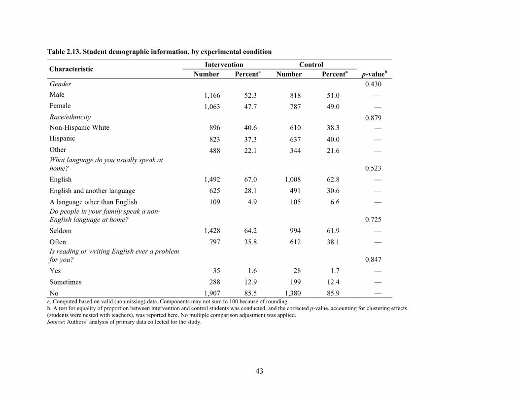
Table 2.13. Student demographic information, by experimental condition

Intervention ControlCharacteristic Number Percenta Number Percenta p-valueb

Gender 0.430 Male 1,166 52.3 818 51.0 — Female 1,063 47.7 787 49.0 — Race/ethnicity 0.879 Non-Hispanic White 896 40.6 610 38.3 — Hispanic 823 37.3 637 40.0 — Other 488 22.1 344 21.6 — What language do you usually speak at home? 0.523 English 1,492 67.0 1,008 62.8 — English and another language 625 28.1 491 30.6 — A language other than English 109 4.9 105 6.6 — Do people in your family speak a non-English language at home? 0.725 Seldom 1,428 64.2 994 61.9 — Often 797 35.8 612 38.1 — Is reading or writing English ever a problem for you? 0.847 Yes 35 1.6 28 1.7 — Sometimes 288 12.9 199 12.4 — No 1,907 85.5 1,380 85.9 —

a. Computed based on valid (nonmissing) data. Components may not sum to 100 because of rounding. b. A test for equality of proportion between intervention and control students was conducted, and the corrected p-value, accounting for clustering effects(students were nested with teachers), was reported here. No multiple comparison adjustment was applied. Source: Authors’ analysis of primary data collected for the study.

43

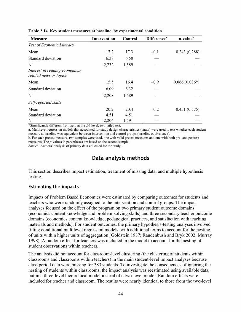
Table 2.14. Key student measures at baseline, by experimental condition

Measure Test of Economic Literacy

Intervention Control Differencea p-valueb

Mean Standard deviation

17.2 6.38

17.3 6.50

–0.1 —

0.243 (0.288) —

N Interest in reading economics-related news or topics

2,232 1,589 — —

Mean 15.5 16.4 –0.9 0.066 (0.036*) Standard deviation 6.09 6.32 — — N 2,208 1,589 — — Self-reported skills Mean Standard deviation

20.2 4.51

20.4 4.51

–0.2 —

0.451 (0.575) —

N 2,204 1,591 — — *Significantly different from zero at the .05 level, two-tailed test. a. Multilevel regression models that accounted for study design characteristics (strata) were used to test whether each studentmeasure at baseline was equivalent between intervention and control groups (baseline equivalence). b. For each pretest measure, two samples were used, one with valid pretest measures and one with both pre- and posttestmeasures. The p-values in parentheses are based on the second sample. Source: Authors’ analysis of primary data collected for the study.

Data analysis methods

This section describes impact estimation, treatment of missing data, and multiple hypothesis testing.

Estimating the impacts

Impacts of Problem Based Economics were estimated by comparing outcomes for students and teachers who were randomly assigned to the intervention and control groups. The impact analyses focused on the effect of the program on two primary student outcome domains (economics content knowledge and problem-solving skills) and three secondary teacher outcome domains (economics content knowledge, pedagogical practices, and satisfaction with teaching materials and methods). For student outcomes, the primary hypothesis-testing analyses involved fitting conditional multilevel regression models, with additional terms to account for the nesting of units within higher units of aggregation (Goldstein 1987; Raudenbush and Bryk 2002; Murray 1998). A random effect for teachers was included in the model to account for the nesting of student observations within teachers.

The analysis did not account for classroom-level clustering (the clustering of students within classrooms and classrooms within teachers) in the main student-level impact analyses because class period data were missing for 383 students. To investigate the consequences of ignoring the nesting of students within classrooms, the impact analysis was reestimated using available data, but in a three-level hierarchical model instead of a two-level model. Random effects were included for teacher and classroom. The results were nearly identical to those from the two-level

44

model.9 For teacher outcomes, single-level regression models were used to estimate program impacts.

All outcome variables were treated as continuous variables in the impact analyses (estimated using multilevel or single-level linear regression models).

To increase the precision of the estimates, a set of baseline characteristics of students and teachers was included in the models as covariates. The following covariates were included in the student outcome analyses:

• Student demographic characteristics: gender (male, female) and race/ethnicity (non-Hispanic White, Hispanic, other).

• Student pretest measure of Test of Economic Literacy.

• Student pretest measure of interest in reading economics-related news or topics.

• Student pretest measure of self-reported skills.

• Teacher-aggregated pretest measure of student scores on Test of Economic Literacy, interest in reading economics-related news or topics, and self-reported skills.

• Teacher pretest measure of Test of Economic Literacy.

• Teacher years of teaching experience, number of college-level economics courses, and confidence in teaching economics concepts.

• Consent process (active or passive).10

• Dichotomous variables for each stratum11 (the dummy codes used to specify which stratum the student was assigned to).

• Missing value indicators (discussed in the following section).

The teacher-level models included the following covariates:

• Teacher demographic characteristics: gender (male, female) and race/ethnicity (non-Hispanic White, Hispanic, other).

• Teacher pretest measure of Test of Economic Literacy.

• Teacher pretest measure of outcome variable (pedagogical practices or satisfaction with teaching materials and methods).

9 The results of the three-level comparative exploratory analysis are available on request from the authors. 10 The majority of the student cohort (93 percent) was engaged in the study under a passive consent process. However, 7 percent of the students participated under active consent in accordance with policy requirements in particular schools or districts. Since the consent process is not under the control of the researchers, it was included in the student impact analysis model to control for a possible difference between intervention and control groups. 11 As indicated earlier in this chapter, before random assignment 15 strata were created and defined by school-level test score data and state (Arizona or California) for the singleton schools. Schools were then randomized within each of the 15 strata. For the 16 schools with two or more teacher participants, each of these schools was their own stratum. Teachers were then randomized within schools (or school strata).

45

• Teacher years of teaching experience, number of college-level economics courses, and confidence in teaching economics concepts.

• Dichotomous variables for each stratum (the dummy codes used to specify which stratum the teacher was assigned to).

• Missing value indicators (discussed in the following section).

A detailed discussion of the model specification is in appendix G.

Treatment of missing data

The missing-indicator method (White and Thompson 2005) was used to account for missing values on the covariates (not the outcome variables) in the impact analysis models. With the missing-indicator method, all observations with missing values on covariates are retained in the analysis. Indicator variables were created for missing values on each variable (0 = observed, 1 = missing), and missing values on the covariates were coded to a constant. Both the recoded covariates and the missing value indicator variables were included in the regression model. In a randomized controlled trial, in which randomization helps ensure that the baseline covariates are balanced, the use of the missing-indicator method appears to refine the precision of impact estimates and standard errors (White and Thompson 2005).

Observations with missing values on outcome variables were excluded from the impact analyses. Deletion of observations with missing outcome variables has been shown to result in accurate impact estimates and standard errors when outcomes are missing at random, conditional on the covariates (Allison 2002; von Hippel 2007).

To examine how robust the findings were with respect to missing data handling procedures, sensitivity analyses (for both student and teacher-level variables) were conducted using different modeling and samples on each outcome variable (see appendix I).

For the Test of Economic Literacy, missing item responses were treated as incorrect responses. For the performance task assessment, items that were assigned a special code of B (blank) or T (out of topic) during scoring were converted to the lowest score point (a score of 1). For the survey scales (from teacher/student surveys), teachers/students who missed one or more items were not included in the analysis.

Multiple hypothesis testing

The procedures described by Schochet (2008) were used to account for multiple hypothesis tests involving the outcome variables assessed in the study. Two outcome domains were delineated at the student level: student content knowledge in economics and student problem-solving skills. Since each student domain only has one outcome measure, multiple comparison procedures were not used within the domain to reduce the probability of finding statistically significant program impacts due to chance factors alone. However, multiple comparison procedures were used for across-domain adjustment. Therefore, the total number of multiple adjustments at the student level is two.

46

At the teacher level, there were three domains, each with a single outcome measure. Therefore, three across-domain adjustments were used. No multiple comparison procedures were used between student-level domains and teacher-level domains since the teacher impacts served as an intermediate outcome variable in the logic model.

Benjamini and Hochberg’s (1995) stepwise multiple hypothesis testing procedure was used to test impact estimates at each level. This procedure involves ordering p-values obtained for each outcome variable across domains at each level (student and teacher) from largest to smallest, multiplying each unadjusted p-value by N/(N – j + 1), where N is the number of primary outcome variables within a domain and j represents the order of the test. The procedure involves rejecting all null hypotheses in which the adjusted p-value is less than .05.

47

3. Implementation of the Problem Based Economics intervention

This chapter discusses the details of the intervention program and implementation costs.

Intervention description

The intervention for this study was a specific set of Problem Based Economics curricular materials provided to intervention group teachers within a professional development and ongoing support program. The teachers used the Problem Based Economics materials as a major portion of their instructional program in their high school economics classes in the 2007/08 academic year.

The curriculum includes space for group discussion, individual work, group tasks, presentations, and end-of-unit assessments, and stresses six core skill sets:

• Managing oneself as an individual: through student and class-based problem logs

• Working as a contributing team member: large and small group work

• Communicating effectively using a variety of methods and technologies: graphs, fliers, presentations, debates, and memos

• Gathering and evaluating data: reading, analyzing, and responding to data and reports

• Making reasoned decisions: making and defending choices

• Understanding interrelationships within school, workplace, and community systems: looking across constituency groups

(Buck Institute for Education 2008)

Curriculum materials

The Problem Based Economics curriculum was developed over many years by the Buck Institute for Education, with the support of university-based economics faculty members. The curriculum comprises nine modules that each take up a particular problem or challenge requiring economic exploration and analysis. For this study, five of the nine modules were provided to the intervention group teachers. The five modules were chosen because they included fundamental components of the curriculum standards in economics in the states where the study was implemented (Arizona and California). The modules were selected by the research team with input from the developers, following a review of the two states’ standards in economics. The Buck Institute developers encourage teachers to use the materials with their other teaching materials and strategies. The intervention in this study was the teachers’ use of the five modules, which covered approximately 50–70 percent of the curriculum content of economics classrooms in the intervention condition.

48

The content of the five modules was as follows:

• Running in Place. Students are asked to explain and illustrate the relationship between producers and consumers of running shoes by assisting a man who wants to start a new business and open a sneaker factory. Student discovery focuses on who makes economic decisions within a free-market economy and how goods and services are produced.

• The Invisible Hand. Students explore how prices are set in a free-market economy and how they serve as the mechanism to distribute goods and services. The case focuses on how to allocate gasoline in a price-controlled market. The students explore the role of government action in economic decision-making and the shortages and surpluses that can emerge in markets under price controls.

• Monopoly’s Might. Students take on the role of entrepreneurs in a school-based enterprise that seeks funding from a venture capitalist to develop a product. The unit challenges students to consider patent rights and the economic implications of monopolists. Students simulate changes in the price, quantity, and profit of their new product over time to model the behavior of firms that enter and exit an industry to compete. The unit examines monopolies to reinforce what is produced, in what quantities, under constrained free-market conditions.

• The Great Awakening. This unit examines comparative advantage and is the mechanism for introducing students to economic considerations of international trade. Students negotiate an international trade agreement that runs into political and social opposition from constituent groups. The unit examines the opportunity costs and the social costs of production decisions within a political context.

• The President’s Dilemma. The unit presents students with a complicated national economy and the associated challenges for government officials and policymakers. In negotiating tax increases and deficit spending policies, students grapple with how societies allocate scarce resources. The students examine policy levers in the economy (such as taxation, government spending, and federal deficits) and the role of stakeholders in how goods and services are produced.

In this experiment, the study team, in consultation with developers, decided to examine the impact on student performance of the use of these five modules with the Buck Institute’s recommended approach to professional development. As a result, the findings of this study cannot be generalized to alternative implementations using different modules, in different combinations, with other forms of support for teachers.

Professional development

The five-day professional development workshop provided to the intervention group familiarized teachers with the curriculum modules, using pedagogical strategies consistent with problem-based instruction. The Buck Institute provided trainers who were current or former economics teachers with substantial experience using the Problem Based Economics curriculum materials. The trainers reviewed one curriculum module each day; pedagogical strategies that are consistently applied in the units were modeled, highlighted, reinforced, and discussed throughout the workshops.

49

Teachers left the session with an understanding of how to sequence the material into eight consistently applied teaching steps (Mergendoller, Maxwell, and Bellisimo 2000):

1. Entry point. Students receive some form of correspondence from the collateral materials that draws them into the problem they are charged with solving.

2. Framing the problem. A strategy is developed to state the problem in a particular way that identifies the content, the actor, and the objective.

3. Knowledge inventory. The teacher leads students in a discussion to assess what they know and what they still need to learn to move forward to solve the problem.

4. Problem log. Students keep track of their progress and what remains to be solved.

5. Research and resources. The teacher provides collateral material and supplemental information periodically throughout the unit to allow ongoing and evolving exploration into the problem.

6. Teachable moments. The teacher serves as a coach to the students, taking measured steps to provide direct instruction and resources to fill in gaps in student knowledge and comprehension.

7. Exit from the problem. Students state their “solution” in the form of a report or group presentation to the class.

8. Wrap-up and debriefing. A teacher-led class discussion reviews the problem-solving strategies that were employed and the utility of competing and alternative solutions and resolutions.

Logistics of the professional development workshops. The study team provided the intervention group teachers with three week-long scheduling options in Phoenix, Sacramento, and Long Beach during summer 2007. Fourteen teachers attended in Phoenix, 15 in Sacramento, and 14 in Long Beach (one teacher split time between the Sacramento and Long Beach trainings). In total, 42 teachers attended the intervention training.

During study recruitment, teachers were told that control group teachers would also be provided with optional Problem Based Economics professional development during the summer of 2008, following completion of data collection for the study. A total of 29 teachers attended the two optional control group training sessions. Control group teachers who chose not to attend either training session were mailed the training materials and curriculum in mid-August 2008.

For the intervention group, the first hour of training was spent taking the Test of Economic Literacy and completing the teacher background survey. For the control group, the pretest and background survey materials were administered by mail in summer 2007 following random assignment.

Ongoing support for teachers throughout the 2007/08 academic year. Intervention teachers had the opportunity to receive ongoing support from the curriculum developer throughout the 2007/08 academic year. On four occasions—at the start of the semester and then roughly timed to the completion of the curriculum modules—teachers participated in a group conference call with the developers and the study team to discuss progress. Teacher participation on these calls varied from a high of 24 to a low of 14. Teachers raised issues of pacing, handling particular content, and juggling other curricular requirements of their schools and districts. They also raised

50

challenges that they had faced and asked for feedback and support. The calls were collegial and afforded the teachers a professional community to discuss challenges with colleagues and trainers. In addition, Buck Institute staff made themselves available by email and phone to answer questions throughout the implementation period. While the study did not collect data on these contacts, anecdotal reports indicate that there were occasional contacts but no large volume of calls or emails.

Intervention implementation costs

The estimated cost for providing the complete array of services to the 42 intervention teachers, including follow-up support, is $206,000. This includes reimbursement of teachers for professional time, materials and training, and logistic support. The estimate assumes that the professional development workshops could be held at a school site or other location without a facility rental fee. In the event that that is not possible, an additional $30,000 would be needed.

Implementation of the study grouped teachers from many schools and school districts. This provided a set of efficiencies and assumes that teacher collaboration has additional benefits to the professional development activities. For this reason, the figures quoted above should be interpreted cautiously if school district officials are trying to estimate the teacher cost for participation on an individual basis.

51

4. Impact results

This section provides the results of the impact analysis organized by the domain structure and research questions presented in chapter 1. Outcomes are presented initially for the primary research questions on student content knowledge in economics and then for the secondary outcomes related to teacher-level impacts. A series of additional analyses are also referenced, with detailed results included in the appendixes.

The confirmatory findings in this study, reported below, are limited to the presentation of intervention contrasts following student outcome measurement at the end of the spring 2008 semester. The outcomes on which the findings are based measured gains for second-semester high school seniors who were taking economics before they graduated from high school. The administration of the outcome measures for this study, which required two hours of testing at the conclusion of the one-semester economics courses, was completed by students in late spring 2008. Students’ participation in the exam was voluntary.

Overview

The analysis presented in this chapter supports a statistically significant finding for the confirmatory outcomes for the two primary (student) research questions. Students whose teachers had received professional development and support in Problem Based Economics outscored their control group peers on the Test of Economic Literacy by an average of 2.6 test items (out of 40 items with the score ranging from zero to 40; effect size = 0.32). For the test of problem-solving skills and their application to real-world economics dilemmas, the outcomes on these student measures also showed significant differences in favor of the intervention group (effect size = 0.27).

The study also supports the following confirmatory outcomes for three secondary (teacher) research questions: no observed differential outcomes between the intervention and control groups on teacher knowledge in economics, no observed differences in teachers’ pedagogical practices with the survey measures used, and statistically significant differences in favor of the intervention group teachers on a measure of satisfaction with the teaching materials and methods (effect size = 1.09).

Student outcomes (primary)

This section answers two research questions in two primary student domains.

Does Problem Based Economics change students’ content knowledge in economics?

The intervention was positively associated with gains in students’ content knowledge in economics, as measured by the Test of Economic Literacy (see table 4.1 and figure 4.1). Adjusted mean differences on the posttest measure of the Test of Economic Literacy for the spring 2008 semester show that the intervention group exceeded the control group,

52

demonstrating a positive intervention contrast (point estimate of 2.60; effect size = 0.32). This difference was significant at the .05 level after adjusting for multiple comparisons across two student-level domains using the Benjamini and Hochberg (1995) adjustment procedure.

One way to interpret the magnitude of this effect is to compare it with the overall progress that students make during an academic or calendar year. Hill et al. (2008) reported that 10th graders’ scores on norm-referenced tests in reading increase by 0.19 standard deviation units and in math by 0.14 standard deviation units over a calendar year.12 If growth in economics achievement is similar, the impact estimates are equivalent to at least one year of growth. We also note that the performance of both the treatment and control groups, on average, was below the national norm for the test for students who took economics in high school (Form B mean score = 25.74; standard deviation = 7.97). (Walstead and Rebeck 2001, p. 17) Table 4.1. Impact analysis of student outcome measures, spring 2008 student cohort

Adjusted means

Impact measure

Intervention (standard deviation)

Control (standard deviation)

Difference (standard

error)

p-value (adjusted p-value)a

95% confidence

interval Effect size

Unweighted student

sample size

Student Test of Economic Literacy

22.61 (8.08)

20.01 (8.21)

2.60* (1.09)

0.017 (0.034) 0.47–4.73 0.32 3,752

Student performance task assessment (composite score)

6.72 (2.11)

6.18 (2.01)

0.54* (0.24)

0.024 (0.024) 0.07–1.01 0.27 3,415

* Significantly different from zero at the .05 level, two-tailed test.Note: Data were regression-adjusted using multilevel regression models to account for differences in baseline characteristics and study design characteristics. Effect sizes were calculated by dividing impact estimates by the control group standard deviation of the outcome variable. a. The Benjamini and Hochberg (1995) procedure was used to calculate adjusted p-values across the two outcome domains. Source: Authors’ analysis of primary data collected for the study.

12 Comparable growth information is not available for high school economics. No similar large-scale intervention studies have been conducted using the Test of Economic Literacy as an outcome measure.

53

54

Figure 4.1. Intervention contrast on student Test of Economic Literacy, spring 2008 student cohort

22.61

20.01

0

10

20

30

40

Spring 2008

Test

of E

cono

mic

Lite

racy

tot

al s

core

Intervention

Control

2.60

Difference

Source: Authors’ analysis of primary data collected for the study.

Does Problem Based Economics change students’ problem-solving skills in economics?

The intervention was also positively associated with gains in students’ problem-solving skills in economics, as measured by the composite score on the performance task assessments (see table 4.1 and figure 4.2). On the composite score developed for analysis of the performance task assessments, the spring 2008 intervention group exceeded the control group, with a positive intervention contrast (point estimate of 0.54; effect size = 0.27). This difference was significant at the .05 level. Adjustment for multiple comparisons across the two student research domains was conducted using the Benjamini and Hochberg (1995) adjustment procedure. Figure 4.2. Intervention contrast on student performance task assessment, spring 2008 student cohort

6.72

6.18

4

6

8

10

12

Spring 2008

Perf

orm

ance

task

ass

essm

ent s

core

Intervention

Control

0.54

Difference

Source: Authors’ analysis of primary data collected for the study.

Teacher outcomes (secondary)

This section answers three research questions in three secondary teacher domains.13

Does Problem Based Economics change teachers’ content knowledge in economics?

The intervention was not associated with teacher gains in economic content knowledge, as measured by the Test of Economic Literacy (see table 4.2). Both intervention and control group teachers were asked to take the Test of Economic Literacy before any professional development began in the summer of 2007. Posttests were administered approximately 10 months later. No significant difference was detected between the intervention and control group teachers on the posttest in spring 2008. Adjusted mean scores for both groups were approximately 37 out of 40 items (the adjusted mean for intervention group teachers was 37.15, versus 36.86 for control group teachers). The analysis was adjusted across the three teacher-level outcome domains using the Benjamini and Hochberg (1995) procedure to account for multiple comparisons. Table 4.2. Impact analysis of teacher outcome measures, spring 2008 semester

Adjusted means

Intervention Control Difference p-value 95% UnweightedImpact (standard (standard (standard (adjusted confidence Effect teacher measure deviation) deviation) error) p-value)a interval size sample size

Teacher Test of Economic Literacy

Pedagogical practices used

Satisfaction with teaching materials and methods

37.15 (3.66)

29.92 (5.09)

8.35 (1.22)

36.86 (1.96)

26.60 (6.00)

6.88 (1.35)

0.29 (0.68)

3.32 (1.78)

1.47** (0.31)

0.675 (0.675) –1.10–1.67 0.15 72

0.070 (0.105) –0.29–6.92 0.55 73

<0.001 (<0.001) 0.84–2.11 1.09 72

**Significantly different from zero at the .01 level, two-tailed test. Note: Data were regression-adjusted using regression models to account for differences in baseline characteristics and study design characteristics. Effect sizes were calculated by dividing impact estimates by the control group standard deviation of the outcome variable. a. The Benjamini and Hochberg (1995) procedure was used to calculate adjusted p-values across the three outcome domains. Source: Authors’ analysis of primary data collected for the study.

13 All available teacher outcome data along with its pretest components from teacher surveys (background survey and end-of-semester survey) are presented in Appendix H. Only the summary statistics (mean and standard deviation for continuous variables or percentages for categorical variables) are reported in Appendix H.

55

56

Does use of Problem Based Economics change economics teachers’ instructional practices?

No significant difference in teachers’ pedagogical practices, as measured through teacher surveys, was observed between the intervention and control groups (see table 4.2). This measure was intended to detect differences in pedagogical practices that are consistent with problem-based instruction and the underlying construction of the Problem Based Economics curriculum. The p-value was adjusted across the three teacher-level outcome domains using the Benjamini and Hochberg (1995) procedure to account for multiple comparisons.

Does use of Problem Based Economics change satisfaction with teaching materials and methods used to teach economics?

The intervention teachers had a higher level of satisfaction with the Problem Based Economics curriculum materials and methods than did the control teachers who used “ordinary” economics teaching materials and teaching methods (see table 4.2 and figure 4.3). The outcome measure satisfaction with teaching materials and methods (point estimate = 1.47; effect size = 1.09) was significant at the .01 level after multiple comparison adjustments across the three outcome domains. Figure 4.3. Intervention contrast on teacher satisfaction with teaching materials and methods, spring 2008 semester

8.35

6.88

2

4

6

8

10

Satis

fact

ion

with

teac

hing

mat

eria

ls &

met

hods

Intervention

Control

1.47

Difference

Source: Authors’ analysis of primary data collected for the study.

Sensitivity analyses

To examine the robustness of the findings, models were estimated with different combinations of baseline covariates for different analytic samples. Because teachers were randomly assigned to the intervention condition, the inclusion of covariates in the impact analysis model should theoretically have consequences for the precision of the impact estimate but not for the point estimate. Changes in point estimates resulting from the inclusion of different sets of covariates

could arise because of baseline differences in characteristics across intervention and control groups. Differences in baseline characteristics, in turn, could be due to chance differences between groups at randomization or to selective attrition after randomization.

Appendix I shows detailed impact analysis results for the primary student outcomes based on regression models that include varying combinations of baseline covariates across different analytic samples.14 The results indicate that the impact estimates do vary when different combinations of covariates are included in the models.

Specifically, as discussed in detail in Appendix I, the differences in point estimates between models that were tested are largely due to intervention-control differences on the teacher baseline TEL measure. For example, we compared the intervention control-contrast for the student TEL outcome (reported in Table 4.1; 2.60) with an alternative specification that removed the teacher baseline TEL from the model as a covariate, all else constant. The resulting contrast for the same outcome was not statistically significant (p = .096); it was reduced to 1.80, or a difference of 0.8.

Acknowledging this sensitivity, we also note that the confidence intervals of all the impact estimates overlap considerably across analytic samples and models that were considered in the sensitivity analyses. Ultimately, the model used to test our primary findings better accounts for random and nonrandom baseline differences between intervention and control groups than the other models and uses the most inclusive student sample available. Thus, the impact estimates and standard errors from the results presented in this chapter appear to be the appropriate estimates.

Limitations of the analyses

As discussed in chapter 2, 45 of the teachers who were randomly assigned to intervention and control groups left the study before data collection, raising concerns about attrition bias. (Information about why teachers left the study is provided in appendix J.) To the extent that these teachers differed from participating teachers, such attrition could reduce external validity (the degree to which the results can be generalized from the remaining teacher sample). Such attrition could also bias impact estimates if the attrition is associated with the study outcome measures and if attrition rates differ between intervention and control groups (What Works Clearinghouse 2008). Causal inferences could also be compromised if the relationships between attrition and study outcomes differ for intervention and control groups. Based on the analyses of equivalence between the intervention and control groups at baseline, and at subsequent points later in the study, there is little evidence of selective attrition. Sensitivity analyses conducted and reported in Appendix I also show consistent findings with varying analytic samples. These

14 Note that the majority of teachers in the final analytic student sample were classified as belonging to “singleton schools” - the only teacher in their school to fully participate in the study. To examine whether the findings for the study were sensitive to “singleton schools”, Appendix I includes analyses that examined impact estimates for student outcomes in only these schools (TEL: point estimate of 3.42; effect size = 0.42; Performance task assessment: (point estimate of 0.71; effect size = 0.36). Based on the results of a Wald test (Judge et al. 1985), these point estimates were not statistically different from those indicated by the main findings presented in this report. Therefore, the findings for this subgroup are consistent with the main findings reported in this chapter indicating that students in PBE classrooms outperformed students in control classrooms.

57

varying samples, reported specifically in Appendix I as panels 1-4, were the result of missing data patterns that followed participant attrition and unresponsiveness to data collection protocols.

However, two caveats are worth noting. First, although attrition and missing data rates were similar for intervention and control teachers, group differences in responsiveness and reasons for dropping out suggest that assignment to condition could have influenced attrition for some teachers. Second, as discussed earlier in this chapter, the impact analysis models are sensitive to which variables are included as covariates. Changes in point estimates resulting from the inclusion of different sets of covariates could arise because of chance differences between groups at randomization or because of selective attrition after randomization. However, there was no direct way to examine whether selective attrition occurred. The primary analytic impact model seemed to provide the most appropriate estimates of program impacts. This model accounts for random and nonrandom baseline differences between intervention and control groups using the data that contained the most information about students and teachers.

58

5. Summary of key findings

This experiment was designed to test whether problem-based instruction in high school economics can result in gains in students’ content knowledge. The analysis at the primary (student) level indicates that students in the spring 2008 semester whose teachers had received professional development and support in Problem Based Economics outscored their control group peers on the Test of Economic Literacy by 2.60 items (effect size = 0.32). Student academic performance was also assessed using open-ended performance tasks that tested problem-solving abilities in short essays. On a composite score of these tasks, students in the intervention group outperformed those in the control group (point estimate of 0.54; effect size = 0.27). This difference was significant at the .05 level after adjusting across the two primary outcome domains to account for multiple comparisons.

The analysis at the secondary (teacher) level indicates no observed differences in teacher knowledge in economics, no observed differences in teachers’ pedagogical style between intervention and control groups with the survey measures used, and statistically significant differences in favor of intervention group teachers on a measure of teacher satisfaction with teaching materials and methods.

These findings add to the nonexperimental research base on Problem Based Economics, which had indicated promising impacts on student gains and teacher satisfaction with the materials. The design underlying this study allows for a causal interpretation of the students’ gains and greater generalizability of findings than the previous research on Problem Based Economics.

Educators may be looking for ways to strengthen their economics education programs. The findings of this study confirm that students benefited from the combination of the professional development program, ongoing support for teachers, and the Problem Based Economics curriculum. At the same time, teachers reported satisfaction with the Problem Based Economics materials. Teachers in the sample had, on average, fewer than three college-level economics courses; the opportunity to engage in a five-day workshop in economics instruction offers support to teachers who are interested in advancing their own professional development and increasing content knowledge..

Generalizability of the findings

During recruitment, the majority of teachers who agreed to participate in the study expressed enthusiasm for the material they taught, its relevance to students’ lives, and the idea that a research study would benefit the profession broadly. Recruitment for the study was not easy, however. Hundreds of economics teachers declined to participate. The original 128 who agreed to participate were interested in finding better ways to reach their students. They included both new and seasoned teachers, with some variation in content expertise. What they had in common was their willingness to participate in the experiment—a selection bias that could not be quantified, but must be acknowledged. This has implications for the generalizability of the study. The results of this study are likely to apply mainly to teachers and schools where the economics program and the associated professional development are a priority. From the perspective of the

59

students, we also note that their participation in the study was voluntary; we cannot quantify whether students unwilling to participate in the economics tests would have performed differently than the study sample described in this report.

Implications for future research

Replication of this experiment is necessary to refine understanding of the impacts associated with the curriculum and the professional development model. The teachers in this study claimed to be satisfied with the Problem Based Economics materials and methods, and yet no significant differences were detected in pedagogical practice between intervention and control group teachers. Additional investigation on measurement in this area is warranted; the survey items used in this study might not have been refined enough to pick up nuances in pedagogical approaches on self-reported data collection.

For example, future study of this curriculum might emphasize classroom observation, to get a clearer understanding of the pedagogical strategies that teachers adopt in varying classroom settings. From observations in intervention and control classrooms, it did not appear to the research team that having and using the problem-based learning curriculum automatically enforced a more hands-on, exploratory classroom learning style. Several times students in the intervention classrooms were observed taking notes on information being delivered through direct instructional approaches—typical of the way high school students record information in most courses that rely on a lecture format (Mergendoller, Maxwell, and Bellisimo, 2000). This could be seen as inconsistent with the curriculum’s intent that students resolve questions through a student-led, problem-based, analytic approach. Additional study in this area might help to refine the pedagogical strategies and allow for additional support and practice for teachers on implementing the curriculum effectively.

A final note: Teachers did not appear to increase their own content knowledge in economics, as measured by the Test of Economic Literacy. In light of the importance of the professional development program and its centrality to the conceptual model, what might explain this finding? The research team made a conscious decision to administer the Test of Economic Literacy to teachers as a pre-post measure, expecting teachers to score well on the assessment. As predicted, the scores on the pretest were, on average, 37 correct answers out of 40, or 93 percent correct. Posttest scores varied little—a point at most, on average. It could be that a ceiling effect on the Test of Economic Literacy instrument masked any true content gains for teachers. In the future, researchers could use teacher content knowledge assessments designed for college-level economics students to allow additional range on the instrument for reflecting any growth in teacher knowledge.

60

Appendix A. Study power estimates based on the final analytic samples

With 64 teachers and an average of 59 students per teacher, the sample size is sufficiently large for detecting substantively meaningful (0.18 standard deviation units) program impacts on academic outcomes for students (see table A.1). For teacher outcomes, the sample size is sufficiently large for detecting larger impacts (0.38–0.46 standard deviation units; see table A.2).

The realized statistical power shown below was equal to or greater than (student and teacher level estimates, respectively) that which was estimated in the planning stage of the study (see Table 2.1) despite there being fewer participating teachers and higher intraclass correlations than expected. This is because the covariates included in the impact analysis models accounted for greater proportions of variance than anticipated at the planning stage of the study.

Table A.1. Minimum detectable effect size for student outcome measures

Total Total

number Average

number of Minimum

Measure number of students

of teachers

students per teacher

Intraclass correlation

detectable effect size

Test of Economic Literacy 3,752 64 59 0.24 0.18

Performance task assessments 3,415 62 55 0.12 0.18

Note: 1. Calculations were estimated based on the following information and assumptions: balanced allocation between intervention and control conditions, statistical power levels of 0.80, Type I error rates of .05 (two-sided), a fixed-effects statistical model, and covariates explained 76 percent of between-teacher variance and 28 percent of within-teacher variance in student scores on the Test of Economic Literacy and 63 percent of between-teacher variance and 12 percent of within-teacher variance in student scores on the performance task assessments. 2. The power estimates presented in table 2.1 were based on the following assumptions that differed from the table above: the number of teachers was 83, the average number of students with valid scores on the Test of Economic Literacy per teacher was 40, the average number of students with valid scores on the performance task assessment per teacher was 16, the intra-class correlation was 0.15 or 0.2, the covariates explained 50% of between- and within-teacher variance in student scores on the Test of Economics Literacy and explained 30% of between- and within-teacher variance in student scores on the performance task assessments. Source: Authors’ analysis of primary data collected for the study.

61

Table A.2. Minimum detectable effect size for teacher outcome measures

Total number of Proportion of variance Minimum

Measure teachers explained by covariates detectable effect size Test of Economic Literacy 72 0.68 0.38

Pedagogical practices used 73 0.57 0.44

Satisfaction with teaching materials and methods 72 0.53 0.46

Note: 1. Calculations were estimated based on the following information and assumptions: balanced allocation between intervention and control conditions, statistical power level of 0.80, Type I error rates of .05 (two-sided), and a fixed-effects statistical model. 2. The power estimates presented in table 2.1 were based on the following assumptions that differ from the table above: the number of teachers was 83 and the covariates explained 20% of the between-teacher variance in each teacher outcome measure. Source: Authors’ analysis of primary data collected for the study.

62

Appendix B. Procedure for assigning new strata to the final analytic sample

As discussed in chapter 2, at random assignment, 15 strata were generated for teachers recruited from a school with only one teacher participant. Another 16 strata were generated for the 16 schools with two or more teacher participants (i.e., each school was its own stratum). Due to teacher attrition after random assignment and/or missing outcome data, several strata were made up of either all intervention or all control group teachers. This poses a problem when the dichotomous variables for “experimental condition” and for “strata” are both included in the impact analysis models. In order to solve this problem, two new strata were created depending on whether the remaining teacher came from a school with multiple participants or from a school with only one participant. Table B.1 shows how many teachers (and the associated number of students) were re-assigned to a new stratum, the reasons they were re-assigned, and how it was done.

As indicated in table B.1, a total of 6 teachers (6 strata) from non-singleton schools were re­assigned to a new stratum #98. This involved a total of 431 students (10% of total 4,350 students in the final analytic sample). On the other hand, a total of 4 teachers (3 strata) from singleton schools were placed into a new stratum #99. This involved a total of 272 students (6% of the final analytic sample). Altogether, 10 teachers (9 strata) with 703 students (16% of the final analytic sample) were re-assigned to new strata.

63

Table B.1. Assigning two new strata to the final analytic sample

Teacher ID Experimental condition

Number of associated students

Number of participating teachers in a school

Original strata at random assignment

New assigned strata for data analysis

Reason for assigning a new stratum

65 Intervention 35 Multiple (3) 31 98 There were three participating teachers in the school/strata at random assignment. One teacher dropped out of study before data collection; another teacher did not teach Economics in the spring semester. Teacher id=65 was the only one teacher remained in strata #31.

66 Intervention 73 Multiple (3) 21 98 Same reason for teacher id=65.

70 Intervention 68 Multiple (2) 22 98 There were two participating teachers in the school/strata at random assignment. One of these two teachers dropped out of study before data collection. Teacher id=70 was the only one teacher remained in strata #22.

104 Intervention 127 Multiple (2) 26 98 Same reason for teacher id=70.

139 Control 66 Multiple (2) 23 98 Same reason for teacher id=70.

147 Control 62 Multiple (2) 30 98 Same reason for teacher id=70.

Total 6 teachers; each came from a school with multiple participating teachers

Total 431 students (10% of total 4,350 students in the final analytic sample)

88 Control 52 1 1 99 There were three participating teachers in the strata at random assignment. These teachers came from different schools. One teacher dropped out of study before data collection; another teacher did not teach Economics in the spring semester. Teacher id=88 was the only one teacher remained in strata #1.

64

Teacher ID Experimental condition

Number of associated students

Number of participating teachers in a school

Original strata at random assignment

New assigned strata for data analysis

Reason for assigning a new stratum

95 Intervention 105 1 15 99 There were two participating teachers in the strata at random assignment. They came from different schools. One of these two teachers dropped out of study before data collection. Teacher id=95 was the only one teacher remained in strata #15.

108 Control 31 1 12 99 There were eight participating teachers in the strata at random assignment. They came from different schools. Six of these teachers dropped out of study before data collection. Teacher id=108 and 130 were the only two teachers remained in strata #12. However, they were both in the control group.

130 Control 84 1 12 99 Same reason for teacher id=108.

Total 4 teachers; Total 272 each came from a singleton school

students (6% of total 4,350 students in the final analytic sample)

65

Appendix C. Scoring procedures for the performance task assessments

This appendix describes the student performance task assessment scoring. WestEd contracted with Educational Data Systems (EDS) for the scoring of the performance task assessments. EDS created the score sheets and contracted with a long-standing partner, the Sacramento County Office of Education (SCOE), to read and score 12,000–15,000 performance task assessments. EDS was the responsible party for scoring discrepancies, data transfers, and related issues. SCOE oversaw the reader and leadership team hiring selection process and the actual reading/scoring process.

All performance task assessments were double-scored, with at least 10 percent read behind by leadership personnel for quality assurance. The performance task assessments were divided among five different essay prompts and scored for four components: conceptual understanding, analysis and reasoning, quantity of relevant supplemental information, and misconceptions or errors. The research team provided CRESST’s rubric, which was modified and made even more precise by SCOE personnel.

Before the formal scoring, the chief reader and the scoring leadership team were brought together in a range-finding meeting to prepare a strategy for training readers to consistently apply the general rubric to each prompt. The meeting included reading hundreds of papers, discussing papers and procedures, gathering papers for use as training materials, and planning for the upcoming scoring session. The final scoring session involved 21 high school economics teachers and 8 leadership team members.

Recruitment

The leadership team included teachers with multiple years of experience in teaching economics and in scoring standardized economics tests, such as the Golden State Examination (GSE) in Economics. The GSE was a test that students took to demonstrate their mastery of the high school curriculum and earn their Golden State Seal Merit Diploma, which “recognized public school graduates who [had] demonstrated their mastery of the high school curriculum in designated content areas” (California Department of Education, 2009, paragraph 2). Experienced high school economics teachers were recruited from across California and screened for appropriate content knowledge and scoring experience. In addition, the research team confirmed that the recruitment pool did not include any teachers who were involved in the impact study.

Familiarization with sample student responses

Two weeks before the scoring session, leadership team members met to familiarize themselves with the student responses, finalize agreement on the application of the general rubric to each prompt, and identify papers to be used in the training and calibration process. The group read and discussed student responses and chose papers to be included in a samples binder. The samples binder contained sample essays for each score point, representing a full spectrum of approaches

66

and writing skills for each component. It also included calibration sets that would be used to check reader calibration at the scoring session. In reading and thoroughly discussing a large sample of examinee responses, the scoring team members calibrated their responses to the scoring guide.

Training

The training included an overview of component scoring and specific requirements of the content guide developed for this prompt. Training staff reviewed the generic rubric in detail so that the readers would be familiar with it when they examined the prompt-specific information.

By design, the initial prompt training took more time than the remaining prompts because readers were becoming accustomed to the generic rubric. During prompt-specific training, the group read and discussed the prompt. All readers received copies of the prompt; the “Content Guide,” which provided specific instructions on how to apply the generic scoring guide to the specific prompt; and the “Behind the Question” document, which explained the key economic concepts of the prompt.

After discussing the anchor papers, readers practiced by scoring two sets of five papers, giving each paper all four component scores. Because few readers were experienced with component scoring, they read the five anchor papers four times—once for each component. Although this process was time consuming, readers more quickly grasped the idea of giving scores on distinct components rather than a single holistic score.

Calibration

Each reader was required to calibrate to the scoring rubric for each of the four components. As in the training, readers considered all four components in scoring the papers.

The first calibration round included 10 papers selected and prescored by the leadership team on each of the four component scores, for a total of 40 scores. Each reader was expected to reach an overall calibration score of 28 out of 40 correct (70 percent), and 6 out of 10 (60 percent) on each component. Scores that differed from the established scores by more than one score point were considered discrepancies.

Readers who did not pass the calibration standard on the first attempt were retrained until they could meet the passing standard on a second, third, or fourth calibration round with five sets of papers each. Calibration standards remained constant (14 out of 20 overall and 3 out of 5 within each component, with no discrepancies). Readers who failed to calibrate successfully were dismissed prior to the scoring process.

Since this format of scoring with a general rubric, across similar prompts, is akin to the CSET®15

(Pearson Education, Inc. 2006) and Praxis16 (Educational Testing Service 2010) examinations,

15 The CSET (California Subject Examinations for Teachers®) program offers educational tests that California uses as part of its teacher licensing/certification process. These include tests for prospective teaching candidates to display competence in single and multiple subjects, writing, technology, and teaching of English learners.

67

their industry-standard model of calibrating readers to the general rubric was followed. Once calibrated on the first prompt, readers were then considered calibrated on all similar prompts unless they demonstrated that they had drifted off calibration. Reader drift was monitored by double-reading by a leadership member and by comparing each reader’s mean scores to those of the group.

Additionally, readers who calibrated on round three or four were put on “probation,” which meant that they needed to demonstrate that they could read consistently for at least two consecutive batches of 10 papers; special readers at each scoring table read behind these batches in their entirety before readers were considered calibrated and ready to read independently.

Thirteen of the 21 readers calibrated on their first attempt. Although 8 of 21 readers failed to calibrate on the first attempt, all but three easily passed the recalibration round after some additional training. Of the three who remained, two eventually calibrated and produced consistent reading once they began on live papers.

Table leaders double-read all of the readers’ first batch of 10 papers to ensure that readers were indeed calibrated and to offer a measure of additional training once the reading began.

Scoring

Once calibrated, but prior to the beginning of the live reading, readers received training on how to move the batches of papers through the room. Readers were assigned unique reader numbers that matched their table and seat location. Readers recorded their reader numbers on the outside of each batch folder and on the batch score sheet.

Each batch contained three different-colored score sheets (white, pink, and yellow), with each color representing a different reading of the paper. All papers were read at least twice; 10 percent were read a third time. To prevent readers from being influenced by the scores of previous readers, after a paper was scored for the first time, its white score sheet was placed in a box designated for Educational Data Systems (EDS).

A document aide would move the batch from the table where it had received its first read to another table in the room for its second read. When the second reader completed reading the batch, the reader moved the pink score sheet to the back of the batch and gave the package to a table leader. The table leaders read behind at least 10 percent of the papers scored by the second reader (one paper per batch).

Read-behinds

Read-behinds were performed in two ways. On batches read by two readers, the table leader received a batch read by a reader at the same table (reader 2) and randomly picked at least one paper from the batch to score. The table leader then read the paper and recorded the score on the yellow score sheet. After recording the score, the table leader checked the second reader’s pink

16 The Praxis Series offers educational tests and services that states use as part of their teacher licensing/certification process. These tests include measurement of basic academic skills, and subject-specific knowledge and teaching skills.

68

score sheet and recorded the second reader’s score alongside his or her own score, keeping a record of agreement.

For some batches, the table leader was the second reader. In these cases, the table leader asked the first reader to leave the white score sheet at the back of the batch. The table leader then read the batch as the second reader and recorded both responses in the read-behind log.

Monitoring

Readers were monitored in several ways. Table leaders watched each reader’s progress using the read-behind logs. If a reader demonstrated any misunderstanding or drift, the table leader provided feedback on the spot and would sometimes read a few extra papers behind the reader. The operations supervisor also made rounds twice a day to check the read-behind logs for each reader. If a reader’s agreement rate fell behind the rate required for calibration, the table leader was asked to begin reading all of the papers of that reader until the reader was again calibrated to the rubric.

At the end of the day, score sheets were sent to EDS to be scanned and processed. EDS would send an electronic file back to the Sacramento County Office of Education, which used the file to monitor individual readers’ scores against those of the group. However, the reading went so quickly that it outpaced this monitoring method because by the time the scoring data were returned, the scoring for a particular prompt had been completed.

Transfers between prompts

After all the papers from one prompt were scored at least twice, the group moved on to the next prompt. After the entire group had been trained on prompt C, the group was split in two. The two groups each read a different prompt. This was done because prompts A and B were similar and the team believed that whichever prompt was read first would cause difficulty for the second. The solution was to split the group and read prompts A and B in separate rooms simultaneously. Before each prompt was read, the readers were retrained to deal with the specifics of the new prompt. They received new training and “behind the question” handouts on the economics involved in the question and a prompt-specific “content guide” on how to consistently apply the general rubric to the prompt they were about to score. Each prompt had a binder containing sample papers that were read, scored, and discussed as part of the training process.

Completion and clean up

Following the scoring session, EDS provided the Sacramento County Office of Education with a list of discrepancies, missed or unscannable scores, and papers that were not clearly defined as either minimal responses or genuine attempts. The chief reader provided a final score for all papers that required attention.

69

Interrater reliability for student performance task assessment

As described earlier, each paper was read and rated (on a three-point scale) by at least two different readers/raters. Tables C.1–C.5 show interrater reliability on the five tasks. Using Table C.1 as an example, the cell of “1” under Reader 1 and “1” under Reader 2 indicates that among 2,495 students who took performance task A, 1,226 papers (corresponding to 49.14 percent of total) received the same rating (i.e., the score of 1); the cell of “2” under Reader 1 and “2” under Reader 2 indicates that 507 papers (20.32 percent) received the same rating (i.e., the score of 2); and the cell of “3” under Reader 1 and “3” under Reader 2 indicates that 176 papers (7.05 percent) received the same rating (i.e., the score of 3). These three cells altogether represent the amount of exact agreement between two ratings. The total “percent exact” equals the sum of these three percentages (49.14, 20.32, and 7.05). If, on the other hand, the rating differed by 1 point (e.g., a score of 1 by Reader 1 but a score of 2 by Reader 2), then the corresponding cell represents the “percent adjacent” (4 cells altogether at each table). The overall percentage agreement (99.12) is equal to the sum of “percent exact” (76.51) and “percent adjacent” (22.61). Table C.1. Interrater analysis on performance task A

Reader 2 1 Percent 2 Percent 3 Percent Total

1 1,226 49.14 134 5.37 6 0.24 1,366 Reader 1 2 214 8.58 507 20.32 107 4.29 828

3 16 0.64 109 4.37 176 7.05 301 Total 1,456 58.36 750 30.06 289 11.58 2,495

Percent exact = 76.51; percent adjacent = 22.61; overall percentage agreement = 99.12; kappa = 0.59; weighted kappa = 0.65. Note: Components may not sum to 100 percent because of rounding. Source: Authors’ analysis of primary data collected for the study.

Table C.2. Interrater analysis on performance task B

Reader 2 1 Percent 2 Percent 3 Percent Total

1 1,903 74.19 122 4.76 11 0.43 2,035 Reader 1 2 95 3.70 260 10.14 51 1.99 407 3 11 0.43 38 1.48 74 2.88 123

Total 2,009 78.32 420 16.38 136 5.30 2,565 Percent exact = 87.21; percent adjacent = 11.93; overall percentage agreement = 99.14; kappa = 0.63; weighted kappa = 0.68. Note: Components may not sum to 100 percent because of rounding. Source: Authors’ analysis of primary data collected for the study.

70

Table C.3. Interrater analysis on performance task C

Reader 2 1 Percent 2 Percent 3 Percent Total

1 586 23.06 102 4.01 3 0.12 691 Reader 1 2 88 3.46 1,031 40.54 101 3.97 1,220 3 3 0.12 101 3.97 528 20.76 632 Total 677 26.64 1,234 48.52 632 24.85 2,543

Percent exact = 84.36; percent adjacent = 15.40; overall percentage agreement = 99.76; kappa = 0.75; weighted kappa = 0.79. Note: Components may not sum to 100 percent because of rounding. Source: Authors’ analysis of primary data collected for the study.

Table C.4. Interrater analysis on performance task D

Reader 2 1 Percent 2 Percent 3 Percent Total

1 790 31.51 136 5.42 1 0.04 927 Reader 1 2 153 6.10 1,320 52.65 39 1.56 1,512 3 3 0.12 26 1.04 40 1.60 69 Total 946 37.73 1,482 59.11 80 3.20 2,508

Percent exact = 85.76; percent adjacent = 14.08; overall percentage agreement = 99.84; kappa = 0.72; weighted kappa = 0.73. Note: Components may not sum to 100 percent because of rounding. Source: Authors’ analysis of primary data collected for the study.

Table C.5. Interrater analysis on performance task E

Reader 2 1 Percent 2 Percent 3 Percent Total

1 934 37.14 330 13.12 9 0.36 1,273 Reader 1 2 217 8.62 537 21.35 149 5.92 903 3 6 0.24 116 4.61 217 8.62 339

Total 1,157 46.00 983 39.08 375 14.90 2,515 Percent exact = 67.11; percent adjacent = 32.29; overall percentage agreement = 99.40; kappa = 0.46; weighted kappa = 0.55. Note: Components may not sum to 100 percent because of rounding. Source: Authors’ analysis of primary data collected for the study.

71

Appendix D. Sample test/survey administration guide

Impact Study:

High School Instruction with Problem Based Economics

End of Semester Data Collection Guide and Samples

For Intervention Teachers

Spring Semester 2008

72

May 2008

Dear Teachers,

We continue to thank you for your effort in the Problem Based Economics study and hope all is going well. At this time, you have already administered the Student Background Survey (SBS) and TEL test to your students. Furthermore, you may have already administered several End of Unit tests. Please continue to administer the End of Unit tests as soon as you finish each unit.

This shipment contains the end of semester testing materials, the administration guides for teachers, and the testing instructions for proctors. In the following pages, you will find an inventory list of your end of semester package materials and a projected timeline of events for the study for the remainder of the semester. For your reference, a sample of the Student End of Semester Survey (SESS) Form A is also included.

Test day one (1) will consist of the Test of Economic Literacy (TEL) test and Student End of Semester Survey (SESS) portion, and test day two (2) will consist of the performance task assessment (PTA) portion. Please note that testing may be administered during one longer session if it would best fit your teaching schedule. However, it is strongly recommended that testing be administered in a two-day setting.

As required by the U.S. Department of Education, a proctor will administer each portion of both test days. This proctor could be a school administrator, a student teacher, or a counselor. Your designated proctor should complete the Proctor Information Form and abide by the enclosed instructions. At the completion of the year, they will receive an Amazon.com gift card as a token of our appreciation.

Should you have any questions, please feel free to contact us at the below numbers or Dr. Neal Finkelstein and his staff at 888.415.ECON (888.415.3226). In assisting with this project, Empirical Education’s goal is to make the data collection process as simple as possible. We encourage you to contact us if you have any concerns, questions, or suggestions.

Thank you again for your participation in the study!

[original contact information for Empirical Education was inserted here]

73

Inventory of materials

Test Day 1 Folder Contents

� Test of Economic Literacy (TEL)—one for each student

� Student End of Semester Survey (SESS) Form A—one for each student

� Scantron answer sheets (2 pages double-sided) with answer sections for the following:

o “Student Information Sheet” (the front of the 1st page)

o “TEL” (the back of the 1st page)

o “Student End of Semester Survey Form A” (the 2nd page, front & back)

Test Day 2 Contents

� Performance Task Assessment (PTA) booklets—one for each student

Outline of data collection activities during the semester

Below is an outline of the end of spring semester’s data collection activities.

There are two main steps for this data collection event:

1. Have a proctor administer the survey/tests

2. Have a proctor return the survey/test answer sheets

Empirical Education will send you the student TEL and Performance Tasks scores by the end of the 2008 summer break. When Event Who April–May 2008 Deliver end of semester data collection instruments Empirical

May 2008 Take TEL, Performance Tasks, and Student End of Semester Survey Students Return student TEL, Performance Tasks, and End of Semester Survey answer sheets as well as Proctor Information Form Proctors

May–June 2008

Complete teacher End of Semester Online Survey (Please let us know if you prefer paper format instead) Teachers

Take the end-of-year teacher assessment Teachers July–August Return student TEL and Performance Tasks scores to teachers Empirical 2008 Return teacher assessment scores to teachers Empirical

74

Appendix E. Teacher-level baseline equivalence tests

Tables E.1–E.3 present the results of teacher-level baseline equivalence tests for additional measures and key teacher baseline measures for the 64 teachers who returned student-level data. Table E.1. Additional teacher measures at baseline, by experimental condition

Measure Self-rated economics knowledge Poor/FairC

Good

InterventionNumber Percenta

11 27.5 22 55.0

Control Number Percenta

5 17.2 16 55.2

p-valueb

0.649 — —

Excellent 7 17.5 7 17.5 — Prefer to teach other subjects rather than economics 0.230 Yes 6 14.6 # # — No 35 85.4 # # —

Willing to teach economics if assigned No # # # #

> 0.99 —

Yes # # # # —

Look forward to teaching economics No # # # #

> 0.99 —

Yes # # # # —

Enthusiastic about teaching economics No 4 9.8 # #

> 0.99 —

Yes 37 90.2 # # — a. Computed based on valid (nonmissing) data. Components may not sum to 100 because of rounding. b. Test was conducted for equality of proportion between intervention and control teachers. No multiple comparison adjustment was applied. c. Poor and Fair categories were collapsed into one category to avoid disclosure risk. However, the Fisher’s exact test on self-rated economics knowledge was based on the original four categories. #: Numbers were removed to avoid disclosure risk. Source: Authors’ analysis of primary data collected for the study.

75

Table E.2. Key teacher measures at baseline for 64 teachers who returned student-level data, by experimental condition

Measure Intervention Control Differencea p-value Test of Economic Literacy pretest Mean 36.4 38.2 –1.8* 0.015 Standard deviation 2.98 1.55 — — N 34 24 — — Years in teaching (any subject) Mean 14.6 14.5 0.1 0.903 Standard deviation 9.83 11.01 — — N 34 24 — — Years in teaching economics Mean 6.9 7.6 –0.7 0.980 Standard deviation 5.93 6.37 — — N 34 24 — — Number of college- or university-level courses in economics Mean 2.8 2.4 0.4 0.382 Standard deviation 1.89 1.64 — — N 34 24 — — Confidence in teaching Mean 43.8 46.6 –2.8 0.153 Standard deviation 7.22 6.95 — — N 33 24 — — Pedagogical practice used Mean 26.2 25.0 1.2 0.336 Standard deviation 5.96 3.83 — — N 32 20 — — Satisfaction with teaching materials and methods Mean 6.1 7.0 –0.9* 0.022 Standard deviation 1.85 1.49 — — N 33 24 — — *Significantly different from zero at the .05 level, two-tailed test. a. Regression models that accounted for study design characteristics were used to test for equivalence between intervention andcontrol groups (baseline equivalence). Source: Authors’ analysis of primary data collected for the study.

76

Table E.3. Additional teacher measures at baseline for 64 teachers who returned student-level data, by experimental condition

Intervention Control Measure Number Percenta Number Percenta p-valueb

Self-rated economics knowledge 0.717 Poor/Fairc 9 27.2 4 16.7 — Good 19 57.6 14 58.3 — Excellent 5 15.2 6 25.0 — Prefer to teach other subjects rather than economics 0.385 Yes 5 14.7 # # — No 29 85.3 # # — Willing to teach economics if assigned >0.99 No # # # # — Yes # # # # — Look forward to teaching economics >0.99 No # # # # — Yes # # # # — Enthusiastic about teaching economics >0.99 No 4 11.8 # # — Yes 30 88.2 # # —

a. Computed based on valid (nonmissing) data. Components may not sum to 100 because of rounding. b. Test was conducted for equality of proportion between intervention and control teachers. No multiple comparison adjustment was applied. c. Poor and Fair categories were collapsed into one category to avoid disclosure risk. However, the Fisher’s exact test on self-rated economics knowledge was based on the original four categories. #: Numbers were removed to avoid disclosure risk. Source: Authors’ analysis of primary data collected for the study.

77

Appendix F. Additional student-level baseline equivalence tests

Tables F.1 and F.2 present the results of additional student-level baseline equivalency tests for categorical and continuous variables.

78

79

Table F.1. Additional student measures at baseline, by experimental condition, categorical variables

Intervention Control p-valuebMeasure Number Percenta Number Percenta

How often do you talk to your friends outside of class about what you are learning in class? Never Once or twice a semester Once a month Once a week Almost every day How often do you try as hard as you can because you are worried about what your friends may think? Never Once or twice a semester Once a month Once a week Almost every day How often do you and your friends study or work together outside of class? Never Once or twice a semester Once a month Once a week Almost every day Which courses are you taking this semester? Any regular courses? Yes No Any college-prep courses? Yes No Any honors courses?

289 400 313 704 523

1,408

308 233 153 119

650 635 488 341 114

1,719 509

1,435

793

13.0 17.9

14.031.6 23.5

63.4 13.9 10.5

6.9 5.4

29.2 28.5 21.9 15.3

5.1

77.2 22.8

64.4 35.6

181 261

231 490 443

1,010

206 183 121

84

428 453 385 258

80

1,237 370

948 659

11.3 16.2 14.4 30.5 27.6

63.0 12.8 11.4

7.5 5.2

26.7 28.2

24.0) 16.1

5.0

77.0 23.0

59.0 41.0

0.321 —

— — — —

0.793 — — — — —

0.621 — — — — — —

0.979 — —

0.463 — —

0.458

80

Intervention Control p-valuebMeasure Number Percenta Number Percenta

Yes 497 22.3 312 19.4 — No 1731 77.7 1,295 80.6 — Any advanced placement courses? 0.662 Yes 780 35.0 528 32.9 — No 1,448 65.0 1,079 67.1 — Any basic courses? 0.242 Yes 502 22.5 312 19.4 — No 1,726 77.5 1,295 80.6 — Any remedial courses? 0.028* Yes 301 13.5 150 9.3 — No 1,927 86.5 1,457 90.7 — Any vocational courses? 0.545 Yes 684 30.7 532 33.1 — No 1,075 66.9 1,544 69.3 — How many hours per day do you expect to do homework this semester, in all your classes? 0.746 No time 70 3.2 57 3.5 — Half an hour or less 429 19.4 302 18.8 — 1 hour 664 29.9 500 31.2 — 2 hours 621 28.0 470 29.3 — 3–4 hours 336 15.2 216 13.5 — 5 or more hours 97 4.4 59 3.7 — What is the course grade you are expecting to receive this semester, in all your classes? 0.131 mostly As 649 29.3 521 32.6 — Mostly Bs 1,041 47.0 778 48.7 — Mostly Cs or lower 524 23.7 300 18.8 — What is the highest degree level you would like to achieve? 0.146 Less than high school degree 8 0.4 4 0.3 — High school degree 218 9.9 114 7.2 —

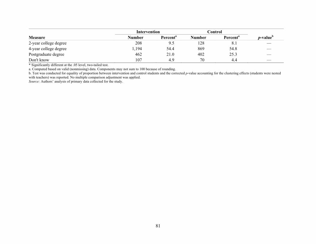
81

Intervention Control p-valuebMeasure Number Percenta Number Percenta

2-year college degree 208 9.5 128 8.1 — 4-year college degree 1,194 54.4 869 54.8 — Postgraduate degree 462 21.0 402 25.3 — Don't know 107 4.9 70 4.4 — * Significantly different at the .05 level, two-tailed test. a. Computed based on valid (nonmissing) data. Components may not sum to 100 because of rounding. b. Test was conducted for equality of proportion between intervention and control students and the corrected p-value accounting for the clustering effects (students were nested with teachers) was reported. No multiple comparison adjustment was applied. Source: Authors’ analysis of primary data collected for the study.

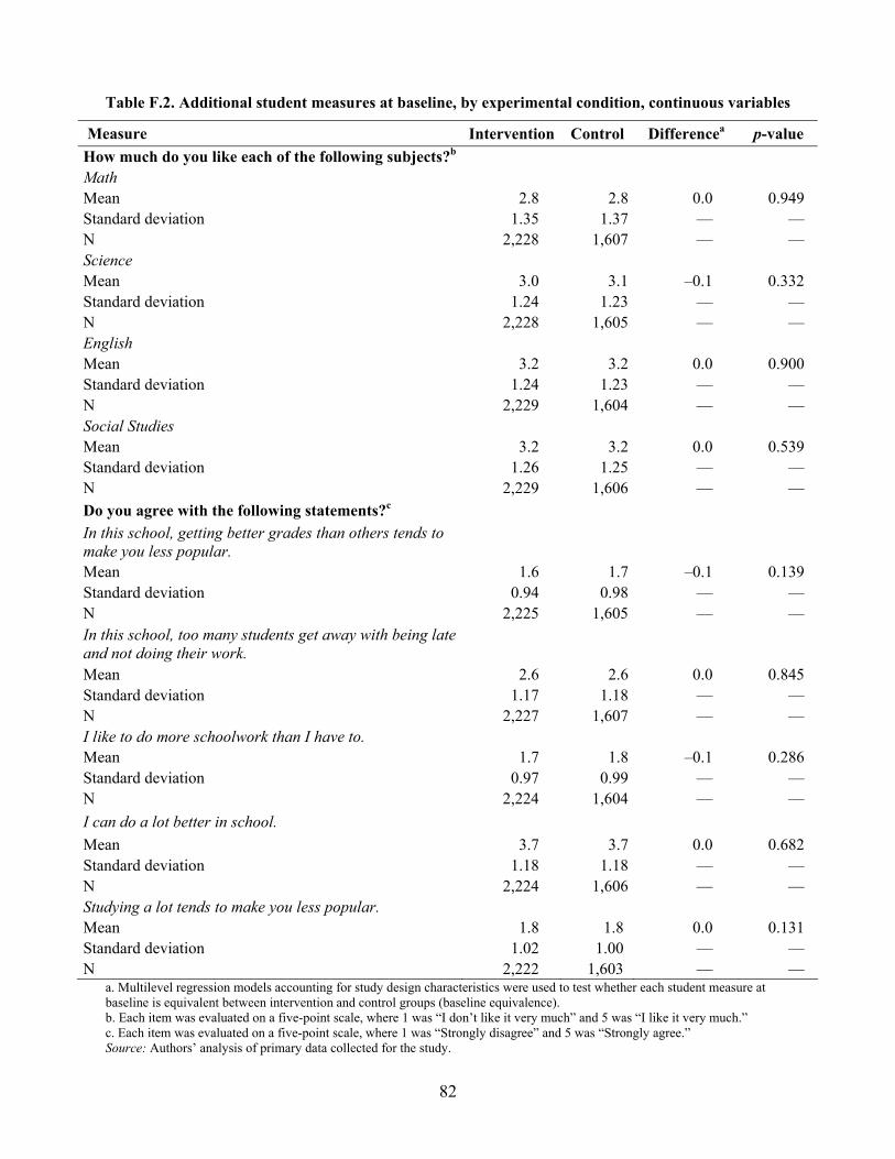
Table F.2. Additional student measures at baseline, by experimental condition, continuous variables

Measure Intervention Control Differencea p-value How much do you like each of the following subjects?b

Math Mean 2.8 2.8 0.0 0.949 Standard deviation 1.35 1.37 — — N 2,228 1,607 — — Science Mean 3.0 3.1 –0.1 0.332 Standard deviation 1.24 1.23 — — N 2,228 1,605 — — English Mean 3.2 3.2 0.0 0.900 Standard deviation 1.24 1.23 — — N 2,229 1,604 — — Social Studies Mean 3.2 3.2 0.0 0.539 Standard deviation 1.26 1.25 — — N 2,229 1,606 — — Do you agree with the following statements?c

In this school, getting better grades than others tends to make you less popular. Mean 1.6 1.7 –0.1 0.139 Standard deviation 0.94 0.98 — — N 2,225 1,605 — — In this school, too many students get away with being late and not doing their work. Mean 2.6 2.6 0.0 0.845 Standard deviation 1.17 1.18 — — N 2,227 1,607 — — I like to do more schoolwork than I have to. Mean 1.7 1.8 –0.1 0.286 Standard deviation 0.97 0.99 — — N 2,224 1,604 — — I can do a lot better in school. Mean 3.7 3.7 0.0 0.682 Standard deviation 1.18 1.18 — — N 2,224 1,606 — — Studying a lot tends to make you less popular. Mean 1.8 1.8 0.0 0.131 Standard deviation 1.02 1.00 — — N 2,222 1,603 — —

a. Multilevel regression models accounting for study design characteristics were used to test whether each student measure at baseline is equivalent between intervention and control groups (baseline equivalence). b. Each item was evaluated on a five-point scale, where 1 was “I don’t like it very much” and 5 was “I like it very much.” c. Each item was evaluated on a five-point scale, where 1 was “Strongly disagree” and 5 was “Strongly agree.” Source: Authors’ analysis of primary data collected for the study.

82

Appendix G. Estimation methods

Chapter 2 briefly described the statistical procedures used to estimate impacts of the Problem Based Economics program. This appendix provides more detail about the statistical methods used to estimate program impacts.

Adjusted post-intervention outcomes for students and teachers in the intervention group were compared with the outcomes for their counterparts in the control group. Using multi-level regression techniques, the primary hypothesis examined whether there were non-random group differences associated with the intervention and, if so, what the magnitude of those differences was. Furthermore, in this study, the data has a nested structure, as students were nested within teachers. From a modeling perspective, therefore, student data in level 1 were nested within the teacher data in level 2, which enables the intervention impacts on students to vary between teachers.

Taking into account this nested data structure, the analysis involved fitting conditional hierarchical linear models with additional terms to account for the nesting of individuals within higher units of aggregation (for example, see Goldstein 1987; Raudenbush and Bryk 2002; Murray 1998). A random effect for teachers was included in the model to account for the nesting of student observations within teachers. Fixed effects included intervention group (a dummy variable indicating whether the student was part of the intervention group or not), baseline (pretest) measures of outcome variables (if available), other student- and teacher-level covariates (to control for the possible group differences at baseline), and missing indicator variables (to handle the missing pretest data/covariates), as discussed in chapter 2.

For student outcomes, the following two-level hierarchical linear model was estimated for each outcome:

(1) Econijk = α0 + β1newPreij + β2dPreij + β3Txjk + ΣβIIijk + ΣβTTjk + ΣβdIdIijk + ΣβdTdTjk + ΣνSStratumk + τ jk + ειjk

where subscripts i, j, and k denote student, teacher, and stratum; Econ represents student economics achievement; newPre represents the baseline measure of the outcome variable with missing values coded to a constant; dPre is the missing indicator for newPre; Tx is a dichotomous variable indicating student enrollment in a teacher’s class who has been assigned to the intervention condition; I and T are vectors of control variables for students and teachers, measured prior to exposure to the intervention (again, the missing values were coded to a constant); dI and dT are vectors of missing indicators for I and T; Stratum represents a vector of fixed effects for k–1 strata; τ represents a random variable for teachers (clustering group); and ε is an error term for individual sample members. The intervention effect is represented by β3, which captures intervention-control differences on the outcome variable after controlling for all covariates and study design factors (strata). Values reported under the “Difference” column in table 4.1 (in chapter 4) correspond to β3 in the associated model estimation at the student level.

Analyses using measures assessed at the teacher level were conducted using models analogous to model 1. For example, for teachers’ economic content knowledge, the following model was used:

(2) TeacherEconjk = α0 + β1newPrej + β2dPrej + β3Txjk + ΣβTTjk + ΣβdTdTjk + ΣνSStratumk + εjk

83

where the subscripts and variables are defined for model 1 except that TeacherEcon represents teacher scores on the Test of Economic Literacy. Note that this model accounts for the nesting of teachers within strata by including dichotomous variables for each of k–1 strata. Similar to the student-level impact analyses, values reported under the “Difference” column in table 4.2 (in chapter 4) correspond to β3 in the associated model estimation at the teacher level.

84

Appendix H. Summary statistics of teacher data from teacher surveys

Table H.1 lists the mean and the standard deviation for three continuous variables that were included in both the teacher background survey and the teacher end-of-semester survey. They are presented by the data collection point (pretest or posttest) and by the experimental status (intervention or control). The pretest statistics for these three variables are identical to those presented in table 2.12 in chapter 2. The posttest statistics are computed based on the same teacher samples that were used for the teacher impact analyses. However, unlike those reported in table 4.2 in chapter 4, the summary statistics presented here are not model-adjusted. Also note that “confidence in teaching” variable was not used as an outcome measure in the teacher impact analyses in this report.

Similarly, table H.2 lists the percentage associated with each response choice for four categorical variables that were included in the teacher surveys. They are again presented by the data collection point and by the experimental status. The pretest information is the same as the one presented in table E.1 in appendix E. These four variables were not used as the outcome measures in the teacher impact analyses in the current report.

Table H.1. Summary of teacher data (continuous variables) from the surveys, by data collection point and experimental condition

Pretest Posttest Measure Intervention Control Intervention Control Confidence in teaching Mean 43.3 46.4 50.4 48.0 Standard deviation 7.94 7.14 5.11 6.04 N 40 29 37 34 Pedagogical practice used Mean 26.1 26.1 30.6 25.9 Standard deviation 5.78 5.03 5.09 6.00 N 39 25 38 35 Satisfaction with teaching materials and methods Mean 6.2 7.0 8.30 6.9 Standard deviation 1.98 1.43 1.22 1.35 N 40 29 37 35 Source: Authors’ analysis of primary data collected for the study.

85

Table H.2. Summary of teacher data (categorical variables) from the surveys, by data collection point and experimental condition

Pretest Posttest Intervention Control Intervention Control

Measure Number Percenta Number Percenta Number Percenta Number Percenta

Prefer to teach other subjects rather than economics Yes 6 14.6 # # 7 18.9 5 14.3 No 35 85.4 # # 30 81.1 30 85.7 Willing to teach economics if assigned No # # # # # # # # Yes # # # # # # # # Look forward to teaching economics No # # # # # # # # Yes # # # # # # # # Enthusiastic about teaching economics No 4 9.8 # # 4 10.5 4 11.4 Yes 37 90.2 # # 34 89.5 31 88.6 Note: a. Computed based on valid (nonmissing) data. Components may not sum to 100 because of rounding. #: Numbers were removed to avoid disclosure risk. Source: Authors’ analysis of primary data collected for the study.

86

Appendix I. Sensitivity of impact estimates to alternative model specifications

To examine the robustness of the findings, models were estimated with different combinations of baseline covariates for different analytic samples. Because teachers were randomly assigned to the intervention condition, the inclusion of covariates in the impact analysis model should theoretically have consequences only for the precision of the impact estimate, not for the point estimate itself. Changes in point estimates could arise from the inclusion of different sets of covariates because of baseline differences in characteristics across intervention and control groups. Differences in baseline characteristics, in turn, could be due to chance differences between groups at randomization or to selective attrition after randomization.

Tables I.1 and I.2 show impact analysis results for the primary student outcomes based on regression models that include varying combinations of baseline covariates across different analytic samples. For student outcomes, program impacts were estimated based on regression models using the following combinations of covariates: randomization strata only; randomization strata, baseline student Test of Economic Literacy (TEL) scores, and an indicator variable for missing data on the baseline student TEL; and all of these covariates plus the student-level and teacher-level covariates described in chapter 2, and indicator variables for missing data on each applicable covariate. These specifications correspond to models A, B, and C in tables I.1 and I.2.

87

Table I.1. Sensitivity of impact estimates to alternative model specification using various sample sets for student content knowledge in economics, spring 2008 student cohort

Adjusted means

Intervention Control Difference p-value 95% Unweighted

Student content knowledge in economics (standard deviation)

(standard deviation)

(standard error)

(adjusted p-value)

confidence interval Effect size

student sample size

Panel 1. Students with nonmissing Test of Economic Literacy posttest data

22.01 20.64 1.37 0.197 Model A (8.08) (8.21) (1.06) (0.394) –0.71–3.45 0.17 3,752

22.24 20.50 1.74 0.050 Model B (8.08) (8.21) (0.89) (0.100) –0.00–3.48 0.21 3,752

22.61 20.01 2.60* 0.017 Model C (8.08) (8.21) (1.09) (0.034) 0.47–4.73 0.32 3,752

Panel 2. Students with nonmissing Test of Economic Literacy pretest and posttest data

22.28 20.89 1.39 0.185 Model A (8.04) (8.21) (1.05) (0.370) –0.66–3.44 0.17 3,382

22.59 20.71 1.88 0.033 Model B (8.04) (8.21) (0.88) (0.066) 0.15–3.61 0.23 3,382

22.86 20.31 2.55* 0.024 Model C (8.04) (8.21) (1.13) (0.048) 0.34–4.75 0.31 3,382

Panel 3. Students with nonmissing Test of Economic Literacy posttest data and nonmissing data on all covariates

22.68 20.96 1.72 0.152 Model A (7.88) (8.15) (1.20) (0.304) –0.63–4.08 0.21 2,878

23.05 20.8 2.24 0.042 Model B (7.88) (8.15) (1.10) (0.084) 0.08–4.41 0.28 2,878

23.29 20.55 2.74 0.033 Model C (7.88) (8.15) (1.28) (0.066) 0.23–5.25 0.34 2,878

88

Adjusted means

Student content knowledge in economics

Intervention (standard deviation)

Control (standard deviation)

Difference (standard

error)

p-value (adjusted p-value)

95% confidence

interval Effect size

Unweighted student

sample size

Panel 4. Students with nonmissing Test of Economic Literacy posttest data (based on 52 teachers in singleton schools)

Model C 22.82 (8.16)

19.40 (8.07)

3.42* (1.33)

0.010 (0.020) 0.81–6.02 0.42 3,262

*Significantly different from zero at the .05 level, two-tailed test. Note: 1. Data were regression-adjusted using multilevel regression models to account for differences in baseline characteristics and study design characteristics. Effect sizes were calculated by dividing impact estimates by the control group standard deviation of the outcome variable. P-values were adjusted across two outcome domains using the Benjamini and Hochberg (1995) procedure. 2. Model specification: Model A: no other covariates except for the strata dummy indicators. Model B: includes pretest of student Test of Economic Literacy plus pretest missing dummy indicator as covariates (in addition to the strata dummy indicators). Model C: includes the following covariates as also listed in chapter 2 (the impact estimate from model C in panel 1 is reported in the main text):

• Student demographic characteristics: gender (male, female) and race/ethnicity (non-Hispanic White, Hispanic, other). • Student pretest measure of Test of Economic Literacy. • Student pretest measure of interest in reading economics-related news or topics. • Student pretest measure of self-reported skills. • Teacher-aggregated pretest measure of student scores on Test of Economic Literacy, interest in reading economics-related news or topics, and self-reported

skills. • Teacher pretest measure of Test of Economic Literacy. • Teacher years of teaching experience, number of college-level economics courses, and confidence in teaching economics concepts. • Consent process (active or passive). • Strata dummy indicators. • Missing value indicators.

Source: Authors’ analysis of primary data collected for the study.

89

Table I.2. Sensitivity of impact estimates to alternative model specification using various sample sets for student performance task assessment, spring 2008 student cohort

Adjusted means

Student performance task assessment (composite score)

Intervention (standard deviation)

Control (standard deviation)

Difference (standard

error)

p-value (adjusted p-value)

95% confidence

interval Effect size

Unweighted student

sample size

Panel 1. Students with nonmissing performance task assessment data

Model A 6.55 (2.11)

6.34 (2.01)

0.21 (0.19)

0.277 (0.277) –0.17–0.59 0.10 3,415

Model B 6.60 (2.11)

6.30 (2.01)

0.30 (0.18)

0.094 (0.094) –0.05–0.64 0.15 3,415

Model C 6.72 (2.11)

6.18 (2.01)

0.54* (0.24)

0.024 (0.024) 0.07–1.01 0.27 3,415

Panel 2. Students with nonmissing performance task composite score and Test of Economic Literacy pretest

Model A 6.56 (2.13)

6.37 (2.02)

0.19 (0.20)

0.339 (0.339) –0.20–0.58 0.09 3,100

Model B 6.62 (2.13)

6.32 (2.02)

0.30 (0.18)

0.101 (0.101) –0.06–0.65 0.15 3,100

Model C 6.75 (2.13)

6.21 (2.02)

0.54* (0.24)

0.026 (0.026) 0.06–1.01 0.27 3,100

90

Adjusted means

Student performance task assessment (composite score)

Intervention (standard deviation)

Control (standard deviation)

Difference (standard

error)

p-value (adjusted p-value)

95% confidence

interval Effect size

Unweighted student

sample size

Panel 3. Students with nonmissing performance task composite score and nonmissing data on all covariates

Model A 6.66 (2.14)

6.36 (2.01)

0.30 (0.23)

0.185 (0.185) –0.14–0.74 0.15 2,657

Model B 6.71 (2.14)

6.32 (2.01)

0.40 (0.21)

0.060 (0.060) –0.02–0.81 0.20 2,657

Model C 6.78 (2.14)

6.29 (2.01)

0.49 (0.26)

0.062 (0.062) –0.03–1.01 0.24 2,657

Panel 4. Students with nonmissing performance task composite score (based on 52 teachers in singleton schools)

Model C 6.78 (2.09)

6.07 (1.98)

0.71* (0.29)

0.015 (0.015) 0.14–1.28 0.36 2,944

*Significantly different from zero at the .05 level, two-tailed test. Note: 1. Data were regression-adjusted using multilevel regression models to account for differences in baseline characteristics and study design characteristics. Effect sizes were calculated by dividing impact estimates by the control group standard deviation of the outcome variable. P-values were adjusted across two outcome domains using the Benjamini and Hochberg (1995) procedure. 2. Model Specification: Model A: no other covariates except for the strata dummy indicators. Model B: includes pretest of student Test of Economic Literacy plus pretest missing dummy indicator as covariates (in addition to the strata dummy indicators). Model C: includes the following covariates as also listed in chapter 2 (the impact estimate from model C in panel 1 is reported in the main text):

• Student demographic characteristics: gender (male, female) and race/ethnicity (non-Hispanic White, Hispanic, other). • Student pretest measure of Test of Economic Literacy. • Student pretest measure of interest in reading economics-related news or topics. • Student pretest measure of self-reported skills. • Teacher-aggregated pretest measure of student scores on Test of Economic Literacy, interest in reading economics-related news or topics, and self-reported

skills. • Teacher pretest measure of Test of Economic Literacy. • Teacher years of teaching experience, number of college-level economics courses, and confidence in teaching economics concepts. • Consent process (active or passive). • Strata dummy indicators. • Missing value indicators.

Source: Authors’ analysis of primary data collected for the study.

91

To ascertain how much the patterns of missing values on the predictor variables might have influenced the results, models A, B, and C were estimated using three different analytic samples: the full analytic sample of students with nonmissing TEL posttest data (panel 1), the subset of students with nonmissing TEL pretest and posttest data (panel 2), and the subset of students with nonmissing TEL posttest data and nonmissing data on all covariates (panel 3). The impact estimates based on model C from the most inclusive student sample (panel 1) are reported in chapter 4 of this report. In addition, since the majority of teachers (52 out of 64) who returned the valid student data came from the singleton schools, we also conducted a sensitivity analysis based on the students from the singleton schools using model C (panel 4) to examine how the point estimates changed (versus the point estimates from panel 1 model C reported in the main text).

The results in panel 1 of table I.1 indicate that the impact estimates do vary when different combinations of covariates are included in the models, but the confidence intervals of all the impact estimates overlap considerably. For the student TEL, the effect of Problem Based Economics reached statistical significance in model C but failed to do so in model B, and the effect size for the model B impact estimate was 0.11 standard deviation units smaller than for model C. Further analyses (not shown in the summary table) indicated that the differences in point estimates between models B and C are almost exclusively due to intervention-control differences on the teacher baseline TEL measure and that the missing dummy indicator for teacher baseline TEL would not have much impact on the point estimate. Excluding the teacher baseline TEL (but keeping the corresponding missing dummy indicator) as a covariate in model C yields an impact estimate of 1.80 (compared with 1.74 for model B—both estimates are not significant at the .05 level). Excluding both the teacher baseline TEL and the corresponding missing dummy indicator results in a point estimate of 1.81, which is very close to 1.80. Similarly, if only the missing dummy indicator for teacher baseline TEL is added to model B, the point estimate would be 1.45 (compared with 1.74 in model B that only includes baseline student TEL scores plus the missing dummy indicator for student baseline TEL—both are not significant at the .05 level). However, including both the teacher baseline TEL and the missing dummy indicator in model B results in impact estimate of 2.34 (p = .013), which is larger than 1.45 or 1.74. Also, this point estimate would be close to the impact estimate of 2.60 in model C.

Panel 2, based on all students with nonmissing TEL pretest and posttest data, shows that including student pretest scores in the model increases the point estimate by 0.06 standard deviation units (model B). Inclusion of the rest of the covariates results in a further 0.08 standard deviation units increase in the point estimate (model C), but the point estimates for model C are similar in panels 1 and 2 (2.60 and 2.55).

Compared with the other analytic samples, the panel 3 results, based on a sample of students with no missing data on covariates, show the most variation in impact estimates, as different combinations of baseline covariates are included in the models. The impact estimate increases from 0.21 to 0.28 standard deviation units as student TEL pretest scores are included in the model (model B), and from 0.28 to 0.34 as other student- and teacher-level covariates are included (model C). This pattern is similar to the results in panels 1 and 2. However, the point estimate from each model in panel 3 is slightly higher than the corresponding ones in panels 1 and 2. In addition, the point estimate of 2.74 for model C (corresponding to 0.34 standard deviation units, compared with 0.32 in panel 1 and 0.31 in panel 2) is not statistically significant

92

after adjusting for multiple comparisons (adjusted p = 0.066 compared with p = 0.033 before adjustment).

Similar to panel 1, additional analyses (not shown in the table) indicated that the differences in point estimates between models B and C in panels 2 and 3 are due mainly to the intervention-control differences in the teacher baseline TEL measure. These results suggest that the procedures used to handle missing data are not responsible for the instability of impact estimates: the patterns of results are similar across the three analytic samples, the same predictor variable (teacher baseline TEL) is largely associated with changes in the impact estimate in the three samples, and the inclusion (for model B)/exclusion (model C) of the missing dummy indicator (for teacher baseline TEL) in the models across three analytical samples does not have much influence on the impact estimate.

The pattern of impact estimates for the student performance task assessment (table I.2) is similar to that for the student TEL. For this outcome, only the estimate from model C is statistically significant in the first two analytic samples. For panels 1 and 2, the estimates from model A are 0.05–0.06 standard deviation units smaller than the estimates from model B, and the estimates from model B are 0.12 standard deviation units smaller than those from model C. For panel 3, the estimate from model A is 0.05 standard deviation units smaller than the estimate from model B. While this is similar to panels 1 and 2, the estimate from model B (0.20) is close to the one from model C (0.24). Similar to the TEL outcome, the point estimate from model C in panel 3 is not statistically significant (adjusted p = 0.062). Separate analyses (not shown in the table) indicate that intervention-control differences in the teacher TEL pretest measure and the teacher-aggregated average student self-reported skills measure account for most of the differences in the impact estimates in models B and C across three analytic samples. As is the case for the student TEL, the inclusion or exclusion of missing data indicator variables (for both teacher baseline TEL and teacher-aggregated average student self-reported skills) in the models have little impact on the point estimates.

Overall, model C and its impact estimates and standard errors, based on the most inclusive analytic samples (panel 1), best account for random and nonrandom baseline differences between the intervention and control groups (note that the standardized point estimates from panels 2 and 3 are similar to those in panel 1). Separate analyses of the larger differences on the impact estimates between models B and C suggest that the differences are affected mainly by the teacher baseline TEL (and the teacher-aggregated average student self-reported skills for the performance task assessment) and not by the missing dummy indicators.

To examine whether the findings for the study were sensitive to “singleton schools”, Panel 4 includes analyses that examined impact estimates for student outcomes in only these schools. The findings are as follows: TEL: point estimate of 3.42 (effect size = 0.42); Performance task assessment: point estimate of 0.71 (effect size = 0.36). Based on the results of a Wald test (Judge et al. 1985), these point estimates were not statistically different from those presented in Panel 1, Model C (Table I.1 and I.2). Therefore, the findings for this subgroup are consistent with the main findings reported in Chapter 4 indicating that students in PBE classrooms outperformed students in control classrooms. Analogous sets of models were estimated for teacher outcomes, but model B included the baseline teacher TEL only, and model C did not include student-level covariates (see table I.3). An additional model, model D, added in response to reviewers’ questions, examines teacher-level impacts for the subset of 63–64 teachers (depending on the outcome measure) used in the

93

student-level impact analyses previously described. As is discussed in chapter 4, there was no evidence that Problem Based Economics affected teacher scores on the TEL or pedagogical practices. The sensitivity analyses indicate that the impact estimates (or effect size) for teacher pedagogical practices are close between models B and C. The impact estimates are not statistically significant at the .05 level in either model B or model C. However, the impact estimate is statistically significant in models A and D. That the impact estimates on teacher pedagogical practices become significant when the analytic sample is restricted to teachers for whom student data are available (model D) is consistent with the notion that differences between teachers for whom student data are and are not available could potentially be responsible for the observed intervention impacts on student outcomes. Without student-level TEL and performance task assessment data from the nine teachers for when these data are not available, there is no way to ascertain this. The results for the other teacher outcomes are relatively stable regardless of how the impact analysis models are specified. In all cases, the confidence intervals for all the impact estimates overlap. As with the student outcomes, the model C results appear to be appropriate

94

Table I.3. Sensitivity of impact estimates to alternative model specification for teacher outcome measures

Adjusted Means Intervention Control Difference p-value 95% Unweighted

Alternative impact models (standard deviation)

(standard deviation)

(standard error)

(adjusted p-value)

confidence interval Effect size

teacher sample size

Teacher Test of Economic Literacy

Model A 36.66 (3.66)

37.41 (1.96)

-0.75 (0.73)

0.307 (0.307) –2.22–0.71 0.38 72

Model B 37.12 (3.66)

36.90 (1.96)

0.22 (0.60)

0.719 (0.719) –0.99–1.42 0.11 72

Model C 37.15 (3.66)

36.86 (1.96)

0.29 (0.68)

0.675 (0.675) –1.10–1.67 0.15 72

Model D 37.25 (3.73)

36.81 (1.57)

0.43 (0.607)

0.480 (0.480) –0.81–1.67 0.28 63

Pedagogical practices used

Model A 30.77 (5.09)

25.68 (6.00)

5.09** (1.33)

<0.001 (<0.001) 2.41–7.76 0.85 73

Model B 29.97 (5.09)

26.55 (6.00)

3.42 (1.64)

0.043 (0.065) 0.12–6.72 0.57 73

Model C 29.92 (5.09)

26.60 (6.00)

3.32 (1.78)

0.070 (0.105) –0.29–6.92 0.55 73

Model D 31.01 (4.62)

26.12 (6.24)

4.90* (1.87)

0.014 (0.021) 1.08–8.71 0.78 64

Satisfaction with teaching materials and methods

Model A 8.34 (1.22)

6.90 (1.35)

1.45** (0.31)

<0.001 (<0.001) 0.82–2.08 1.07 72

Model B 8.16 (1.22)

7.09 (1.35)

1.06* (0.37)

0.006 (0.018) 0.32–1.81 0.79 72

Model C 8.35 (1.22)

6.88 (1.35)

1.47** (0.31)

<0.001 (<0.001) 0.84–2.11 1.09 72

Model D 8.44 (1.29)

6.82 (1.43)

1.62** (0.33)

<0.001 (<0.001) 0.94–2.30 1.14 63

*Significantly different from zero at the .05 level, two-tailed test. **Significantly different from zero at the .01 level, two-tailed test.

95

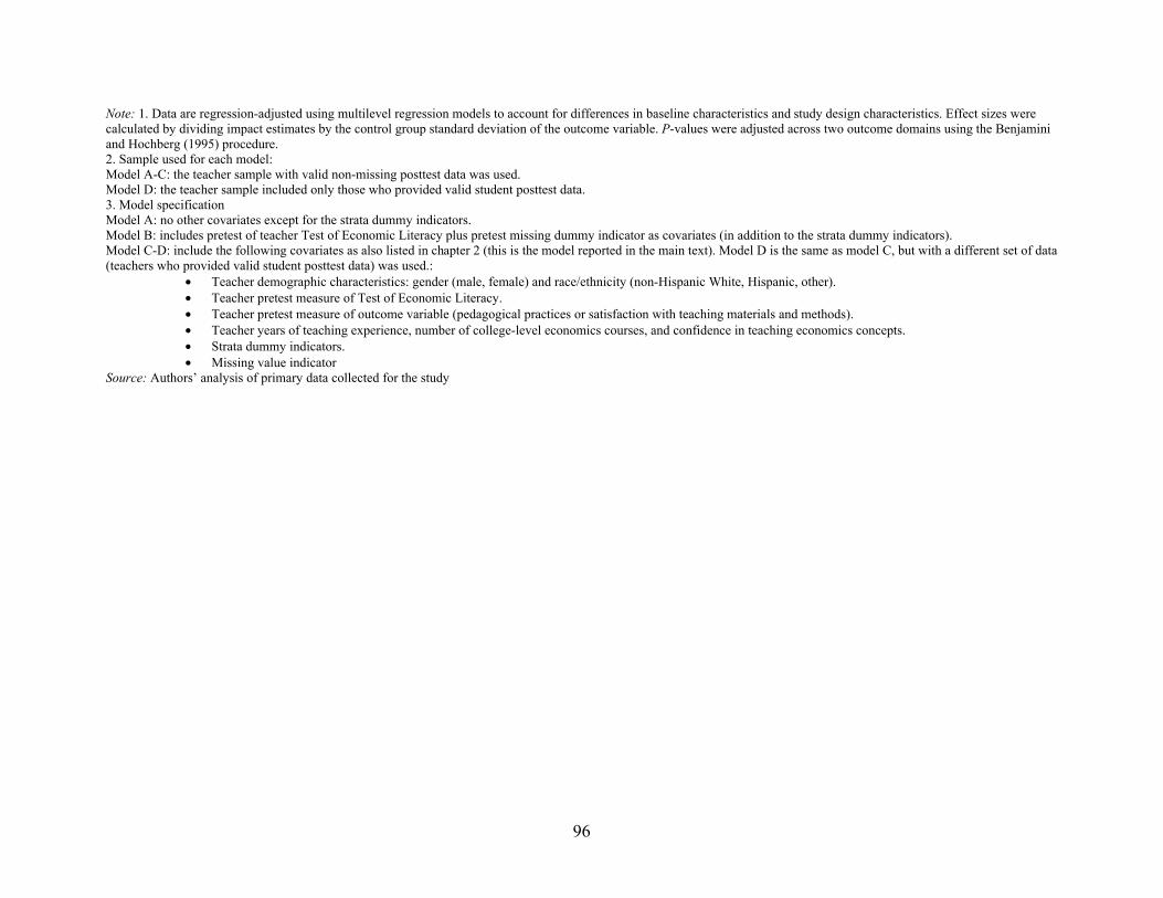
Note: 1. Data are regression-adjusted using multilevel regression models to account for differences in baseline characteristics and study design characteristics. Effect sizes were calculated by dividing impact estimates by the control group standard deviation of the outcome variable. P-values were adjusted across two outcome domains using the Benjamini and Hochberg (1995) procedure. 2. Sample used for each model: Model A-C: the teacher sample with valid non-missing posttest data was used. Model D: the teacher sample included only those who provided valid student posttest data. 3. Model specification Model A: no other covariates except for the strata dummy indicators. Model B: includes pretest of teacher Test of Economic Literacy plus pretest missing dummy indicator as covariates (in addition to the strata dummy indicators). Model C-D: include the following covariates as also listed in chapter 2 (this is the model reported in the main text). Model D is the same as model C, but with a different set of data (teachers who provided valid student posttest data) was used.:

• Teacher demographic characteristics: gender (male, female) and race/ethnicity (non-Hispanic White, Hispanic, other). • Teacher pretest measure of Test of Economic Literacy. • Teacher pretest measure of outcome variable (pedagogical practices or satisfaction with teaching materials and methods). • Teacher years of teaching experience, number of college-level economics courses, and confidence in teaching economics concepts. • Strata dummy indicators. • Missing value indicator

Source: Authors’ analysis of primary data collected for the study

96

Appendix J. Explanations for sample attrition

This appendix presents the reasons for sample attrition by experimental condition. Table J.1. Explanation for sample attrition by assigned status

Intervention Control Total

Reason Number Percent Number Percent Number Percent

Personal issues # # # # # #

Position change

Schedule issues

#

9

#

40.91

#

7

#

30.43

#

16

#

35.56

Refuse to answer

# # 14 60.87 # #

Cannot attend summer training

8 36.36 — — 8 17.78

Total 22 100.00 23 100.00 45 100.00 Note: When the eight intervention teachers who could not attend summer training are excluded (intervention teachers only), the statistical test of differences in the reasons for leaving the study (based on the remaining 37 teachers) was significant at the .05 level (p = .022 based on the Fisher’s exact test). Further examination of the frequency distribution table shows that more control teachers than intervention teachers refused to provide reasons for leaving the study, causing the test to be significant. #: Numbers were removed to avoid disclosure risk. Source: Authors’ analysis of primary data collected for the study.

97

References

Achilles, C.M., and Hoover, S.P. (1996). Exploring problem-based learning (PBL) in grades 6– 12. Retrieved September 10, 2009, from http://www.eric.ed.gov/ERICWebPortal/contentdelivery/servlet/ERICServlet?accno=ED406 406

Allison, P.D. (2002). Missing data. Thousand Oaks, CA: Sage Publications.

Artino, A. (2008). A brief analysis of research on problem-based learning. Retrieved September 10, 2009, from http://www.eric.ed.gov/ERICWebPortal/contentdelivery/servlet/ERICServlet?accno=ED501 593

Baker, E.L. (1997). Model-based performance assessment. Theory into Practice, 36, 247–54.

Baker, E. L., Aschbacher, P. R., Niemi, D., and Sato, E. (1992). CRESST performance assessment models: assessing content area explanations. Retrieved April 21, 2010, from http://www.cse.ucla.edu/products/guidebooks/cmodels.pdf

Baker, E.L., Freeman, M., and Clayton, S. (1991). Cognitive assessment of history for large-scale testing. In M.C. Wittrock and E.L. Baker (Eds.), Testing and cognition. Englewood Cliffs, NJ: Prentice-Hall.

Baker, E.L., Linn, R.L., Abedi, J., and Niemi, D. (1996). Dimensionality and generalizability of domain-independent performance assessments. Journal of Educational Research, 89(4), 197–205.

Baker, E.L., and Mayer, R.E. (1999). Computer-based assessment of problem solving. Computers in Human Behavior, 15(3), 269–282.

Benjamini, Y., and Hochberg, Y. (1995). Controlling the false discovery rate: a new and powerful approach to multiple testing. Journal of the Royal Statistical Society, Series B, 57(1), 1289–1300.

Bernanke, B.S. (2006). Testimony of Chairman Ben S. Bernanke on Financial Literacy before the Committee on Banking, Housing, and Urban Affairs of the United States Senate. Washington, DC: Federal Reserve Board. Retrieved September 10, 2009, from http://www.federalreserve.gov/boarddocs/testimony/2006/20060523/default.htm

Bridges, E. (1992). Problem based learning for administrators. ERIC Clearinghouse on Educational Management, University of Oregon (ED 347617). Retrieved September 10, 2009, from

98

http://www.eric.ed.gov/ERICDocs/data/ericdocs2sql/content_storage_01/0000019b/80/24/31 /a6.pdf

Buck Institute for Education. (2008). Problem Based Economics (curriculum). Retrieved September 10, 2009, from http://www.bie.org/index.php/site/PBE/pbe_overview/

California Department of Education. (2008). API data files 2006. Retrieved May 15, 2008, from http://www.cde.ca.gov/ta/ac/ap/apidatafiles.asp

California Department of Education. (2009). Questions and Answers: Standardized Testing and Reporting (STAR). Retrieved January 26, 2010, from http://www.cde.ca.gov/ta/tg/sr/gsefaq.asp

Duch, B. (1995). What is problem-based learning? About teaching 47. A newsletter of the Center for Teaching Effectiveness. Retrieved September 10, 2009, from http://www.udel.edu/pbl/cte/jan95-what.html

Duvall, R.F. (2009). Federal government’s role in empowering Americans to make informed financial decisions. Testimony before the Senate Subcommittee on Oversight of Government Management, the Federal Workforce, and the District of Columbia, April 29, 2009. Retrieved September 10, 2009, from http://www.councilforeconed.org/news/story.php?story_id=157

Educational Testing Service. (2010). The Praxis Series: Teacher Licensure and Certification. Retrieved January 8, 2010, from http://www.ets.org/portal/site/ets/menuitem.fab2360b1645a1de9b3a0779f1751509/?vgnextoi d=48c05ee3d74f4010VgnVCM10000022f95190RCRD

Expeditionary Learning Outward Bound. (1999). Early indicators from schools implementing New American Schools designs. Cambridge, MA: Expeditionary Learning Outward Bound.

Gijselaers, W.H. (1996). Connecting problem-based practices with educational theory. New Directions for Teaching and Learning, (68), 13–21.

Goldstein, H. (1987). Multilevel models in educational and social research. London: Oxford University Press.

Hendrie, C. (2003). Small schools hard to start, report finds. Education Week, 22(32). Retrieved September 10, 2009, from http://www.edweek.org/ew/articles/2003/04/23/32gates.h22.html

Hill, C.J., Bloom, H.S., Black, A.R., and Lipsey, M.W. (2008). Empirical benchmarks for interpreting effect sizes in research. Child Development Perspectives, 2(3), 172–77.

Hmelo-Silver, C.E., Duncan, R.G., and Chinn, C.A. (2007). Scaffolding and achievement in problem-based and inquiry learning: a response to Kirschner, Sweller, and Clark (2006). Educational Psychologist, 42(2), 99–107.

99

Honey, M., and Henríquez, A. (1996). Union City interactive multimedia education trial: 1993– 95 summary report (CCT Reports, 3). Retrieved September 10, 2009, from http://www.edc.org/CCT/ccthome/tech_rept/CCTR3/

Judge, G. G., Griffiths, W. E., Hill, R. C., Lutkepohl, H. and Lee, T.-C. (1985). The Theory and Practice of Econometrics. (2nd ed.) New York: Wiley.

Kirschner, P.A., Sweller, J., and Clark, R.E. (2006). Why minimal guidance during instruction does not work: an analysis of the failure of constructivist, discovery, problem-based, experiential, and inquiry-based teaching. Educational Psychologist, 41(2), 75–86.

Landis, J.R., and Koch, G.G. (1977). The measurement of observer agreement for categorical data. Biometrics 33(1), 159–74.

Lopus, J., and Placone, D. (2002). Online stock market games for high schools. Journal of Economic Education, 33(2), 192.

Massa, N.M. (2008). Problem-based learning (PBL): a real-world antidote to the standards and testing regime. New England Journal of Higher Education, 22(4), 19–20.

Maxwell, N., Mergendoller, J., and Bellisimo, Y. (2005). Problem-based learning and high school macroeconomics: a comparative study of instructional methods. The Journal of Economic Education, 36(4), 315–31. Retrieved September 10, 2009, from http://www.bie.org/files/PBE%20JEE%20paper_1.pdf

Memory, D.M., Yoder, C.Y., Bolinger, K.B., and Wilson, W.J. (2004). Creating thinking and inquiry tasks that reflect the concerns and interests of adolescents. Social Studies, 95(4), 147.

Mergendoller, J., Maxwell, N., and Bellisimo, Y. (2000). Comparing problem-based learning and traditional instruction in high school economics. The Journal of Educational Research, 93(6), 374–82.

Mergendoller, J., Maxwell, N., and Bellisimo, Y. (2006). The effectiveness of problem-based instruction: a comparative study of instructional methods and student characteristics. Interdisciplinary Journal of Problem-based Learning, 5(2), 5. Retrieved September 10, 2009, from http://docs.lib.purdue.edu/ijpbl/vol1/iss2/5/

Mo, K., and Choi, Y. (2003). Comparing problem-based learning with traditional instruction: focus on high school economics. Theory and Research in Citizenship Education, 35(1), 89– 113. Published by the Association of Social Education in Korea (ISSN: 1598-7280). English abstract is available at http://www.bie.org/index.php/site/resource/item150 (retrieved September 10, 2009).

Moeller, B. (2005). Understanding the implementation of problem-based learning in New York City high school economics classrooms. In J. Ravitz (Chair), Assessing implementation and impacts of PBL in diverse K–12 classrooms. Paper presented at the annual meeting of the

100

American Educational Research Association, Montreal, Canada. Retrieved February 2, 2010, from http://www.bie.org/research/study/understanding_the_implementation_of_problem­based_learning_in_new_york_city

Murray, D.M. (1998). Design and analysis of group randomized trials. New York: Oxford University Press.

National Assessment of Educational Progress. (2007). The nation’s report card: economics 2006. Retrieved September 10, 2009, from http://nces.ed.gov/pubsearch/pubsinfo.asp?pubid=2007475

National Council on Economic Education. (1997). Voluntary national content standards in economics. New York: National Council on Economic Education.

National Council on Economic Education. (1999). Standards in economics: survey of students and the public. New York: National Council on Economic Education. Retrieved September 10, 2009, from http://www.councilforeconed.org/cel/results.php

National Council on Economic Education. (2007). Economic, personal finance & entrepreneurship education in our nation’s schools in 2007. A report card: survey of the states. New York: National Council on Economic Education. Retrieved September 10, 2009, from http://www.councilforeconed.org/about/survey2007/NCEESurvey2007.pdf

Newmann, F., and Wehlage, G. (1995). Successful school restructuring: a report to the public and educators by the Center on Organization and Restructuring of Schools. Madison, WI: Wisconsin Center for Education Research. Distributed jointly by the American Federation of Teachers, Association for Supervision and Curriculum Development, National Association of Elementary School Principals, and the National Association of Secondary School Principals.

Niemi, D. (1996). Assessing conceptual understanding in mathematics: representation, problem solutions, justifications, and explanations. Journal of Educational Research, 89(6), 351–63.

O’Neil, H.F., Jr. (1999). Perspectives on computer-based performance assessment of problem solving: editor’s introduction. Computers in Human Behavior, 15(3–4), 255–68.

Pearson Education, Inc. (2006). California Subject Examinations for Teachers® Test Guide. Amherst, MA: Pearson Education, Inc. Retrieved January 11, 2010, from http://www.cset.nesinc.com/PDFs/CS_testguide_geninfo.pdf

Raudenbush, S.W., and Bryk, A.S. (2002). Hierarchical linear models: applications and data analysis methods (2nd ed.). Thousand Oaks, CA: Sage Publications.

Raudenbush, S. W., Martinez, A., Spybrook, J. (2005). Strategies for improving precision in group-randomized experiments. New York: William T. Grant Foundation.

101

Ravitz, J., and Mergendoller, J. (2005). Evaluating implementation and impacts of problem based economics in U.S. high schools. In J. Ravitz (Chair), Assessing implementation and impacts of PBL in diverse K–12 classrooms. Paper presented at the annual meeting of the American Educational Research Association, Montreal, Canada. Retrieved September 10, 2009, from http://www.bie.org/AERA2005/Ravitz_Mergendoller.pdf

Ravitz, J., Becker, H., & Wong, Y. (2000). Constructivist compatible beliefs and practices among U.S. teachers: Teaching, Learning & Computing, 1998 National Survey, Report #4. UC, Irvine. Retrieved September 10, 2009, from http://www.crito.uci.edu/tlc/findings/report4/report4.pdf

Schochet, P.Z. (2008). Guidelines for multiple testing in impact evaluations of educational interventions (MPR Reference No. 6300-080). Princeton, NJ: Mathematical Policy Research, Inc.

Schug, M.C., Dieterle, D.A., and Clark, J.R. (2009). Are high school economics teachers the same as other social studies teachers? The results of a national survey. Social Education 72(2) 71–75. Retrieved October 10, 2009, from http://markschug.com/pdf/AreHighSchoolEconTeachersTheSame.pdf

Siegfried, J.J., and Meszaros, B.T. (1998). Voluntary economics content standards for America’s schools, Journal of Economic Education, 29(2), 139–49.

StataCorp. (2007). Stata statistical software: release 10. College Station, TX: StataCorp LP.

Stigler, G.J. (1970). The case, if any, for economic literacy. Journal of Economic Education, 1(2), 77–84.

Tobin, J. (1986). Economic literacy isn’t a marginal investment. Wall Street Journal New York: July 9, 1986

U.S. Department of Education. (2010). Excellence in Economics Education Awards. Retrieved January 11, 2010, from http://www.ed.gov/programs/econeducation/awards.html

U.S. Department of Education. (2001). Excellence in Economics Education Act of 2001. Retrieved September 10, 2009, from http://www.ed.gov/policy/elsec/leg/esea02/pg78.html

University of California, Los Angeles, National Center for Research on Education, Standards, and Student Testing (UCLA CRESST). (2005). High School Economics Performance Assessments. Los Angeles, CA: UCLA.

von Hippel, P.T. (2007). Regression with missing Y’s: an improved strategy for analyzing multiply imputed data. Sociological Methodology, 37(1), 83–117.

Walstad, W.B. (2001). Economic education in U.S. high schools. Journal of Economic Perspectives, 15(3), 195–210.

102

Walstad, W.B. (2007). Five developments advancing economic education in the United States: the role of the National Council on Economic Education. Comments for a panel session at the annual meeting of the National Council on Economic Education, National Association of Economic Educators, and Global Association of Teachers of Economics, Denver. Retrieved September 10, 2009, from http://www.councilforeconed.org/news/story.php?story_id=116

Walstad, W.B., and Rebeck, K. (2001). Examiners Manual, Test of Economic Literacy, Third Edition. New York: National Council on Economic Education.

Watts, M. (2006). What works: a review of research on outcomes and effective program delivery in precollege economic education. New York: National Council on Economic Education.

What Works Clearinghouse. (2008). Procedures and standards handbook (version 2.0). Retrieved September 13, 2009, from http://ies.ed.gov/ncee/wwc/pdf/wwc_procedures_v2_standards_handbook.pdf

White, I.R., and Thompson, S.G. (2005). Adjusting for partially missing baseline measurements in randomized trials. Statistics in Medicine, 24(77), 993–1007.

Winick, D.M. (2007). Statement on results from The nation’s report card: Economics 2006. Washington, DC: National Assessment Governing Board, August 8, 2007. Retrieved January 11, 2010, from http://www.nagb.org/newsroom/PressReleasePDFs/Economics%202006%20­%20Winick%20statement.pdf

103

www.ed.gov ies.ed.gov