effects of strong-motion duration on the response of
TRANSCRIPT

Effects of Strong-motion Duration on the Response
of Reinforced Concrete Frame Buildings
Mazen Sarieddine
A Thesis
in
The Department
of
Building, Civil and Environmental Engineering
Presented in Partial Fulfillment of the Requirements
for the Degree of Master of Applied Science (Civil Engineering) at
Concordia University
Montreal, Quebec, Canada
November 2013
© Mazen Sarieddine, 2013

CONCORDIA UNIVERSITY School of Graduate Studies
This is to certify that the thesis prepared
By: Mazen Sarieddine
Entitled: Effects of Strong-motion Duration on the Response of Reinforced Concrete
Frame Buildings
and submitted in partial fulfillment of the requirements for the degree of
Master of Applied Science (Civil Engineering)
complies with the regulations of the University and meets the accepted standards with
respect to originality and quality.
Signed by the final examining committee:
Chair
Dr. K. Galal
Examiner
Dr. R. Ganesan
Examiner
Dr. L. Tirca
Supervisor Dr. L. Lin
Approved by
Chair of Department or Graduate Program Director
Dean of Faculty
Date

iii
Abstract
Effects of Strong-motion Duration on the Response of
Reinforced Concrete Frame Buildings
Mazen Sarieddine
In current practice of the selection of earthquake records for the time-history
analysis of structures, the parameters considered are earthquake magnitude, distance from
the earthquake source to the site where the record is obtained, soil condition at the site,
and type of earthquake. The strong-motion duration of the record is not considered in
this process. A number of studies have been conducted on the investigation of the effects
of strong-motion duration on the structural response; however the conclusions from these
studies are contradictory. Some studies report significant effects while others report
minimal or no effects. The objective of this study was to investigate the effects of strong-
motion duration of earthquake records on the seismic response of reinforced concrete
frame buildings.
For the purpose of the study, three reinforced concrete frame buildings (4-, 10-,
and 16-storey) designed according to the 2005 edition of the National Building Code of
Canada were considered in the analyses. The buildings were located in Vancouver, which
is in a high seismic zone in Canada. Nonlinear time-history analyses were conducted on
three building models using two sets of accelerograms as seismic excitations. One set
consists of simulated accelerograms representative of the ground motions in Vancouver,
and the other set consists of real accelerograms recorded from earthquakes in California.
The ground motions were scaled to three excitation levels, i.e., 0.5Sa(T1), 1.0Sa(T1), and
2.0Sa(T1) in which Sa(T1) was the spectral acceleration at the dominant period of the

iv
building. The four definitions of strong-motion duration considered in the study were
uniform duration, bracketed duration, significant duration, and effective duration. The
structural responses were represented by interstorey drift, beam curvature ductility,
column curvature ductility, roof displacement and base shear.
Based on the results from the study, it was found that the effects of the strong-
motion duration on the structural response depended on the dynamic characteristics of the
building and the seismic excitation level. They did not depend on the response parameter
considered and the type of the record used in the analysis. Moreover, regression functions
between the structural response and the strong-motion duration could not be developed
with respect to the response parameters and the definitions of the strong-motion duration
considered in this study.

v
Acknowledgments
I would like to express my sincere gratitude to my supervisor Dr. Lan Lin for her
continuous support and patience during the course of this study.
I am also thankful for my family, for their support, love, and encouragement that
helped me throughout my study at Concordia University.

vi
Table of Contents
List of Tables…………………………………….………………….……viii
List of Figures…..…………………………….………………........……....ix
Chapter 1: Introduction……………..……………………………….…….1
1.1 Motivation ..................................................................................................................... 1
1.2 Objective and Scope of the Study ................................................................................. 3
1.3 Outline of the Thesis ..................................................................................................... 4
Chapter 2: Literature Review……………………………………………...6
2.1 Introduction……………………………………………………………………………6
2.2 Review the Effects of the Strong-motion Duration on the Structural Response .......... 7
2.3 Review the Definitions of Strong-motion Duration.................................................... 11
2.3.1 Uniform duration ............................................................................................... 11
2.3.2 Bracketed duration ............................................................................................. 11
2.3.3 Significant duration ............................................................................................ 12
2.3.4 Effective duration............................................................................................... 13
Chapter 3: Design and Modelling of Frames……………………………17
3.1 Description of Buildings ............................................................................................. 17
3.2 Design of Frames ........................................................................................................ 18
3.3 Modelling of Frames for Dynamic Analysis .............................................................. 20
Chapter 4: Selection of Earthquake Records….………………………...28
4.1 Overview of the Seismic Hazard for Vancouver ........................................................ 28
4.2 Predominant Magnitude-distance Scenarios for Vancouver ....................................... 29
4.3 Selection of Records ................................................................................................... 31
4.3.1 Simulated records............................................................................................... 31
4.3.2 Real records ....................................................................................................... 33
Chapter 5: Analysis Results from Simulated Records.………………….40
5.1 Overview of Analyses and Response Parameters ....................................................... 40
5.2 Seismic Performance of Frames ................................................................................. 42

vii
5.2.1 Interstorey drift .................................................................................................. 42
5.2.2 Beam curvature ductility .................................................................................... 48
5.2.3 Column curvature ductility ................................................................................ 53
5.2.4 Roof displacement ............................................................................................. 57
5.2.5 Base shear .......................................................................................................... 60
5.3 Effects of Strong-motion Duration on the Structural Response ................................. 63
5.3.1 Interstorey drift .................................................................................................. 64
5.3.2 Beam curvature ductility .................................................................................... 68
5.3.3 Column curvature ductility ................................................................................ 72
5.3.4 Roof displacement ............................................................................................. 75
5.3.5 Base shear .......................................................................................................... 78
Chapter 6: Analysis Results from Real Records.……………................113
6.1 Introduction ............................................................................................................... 113
6.2 Effects of Strong-motion Duration on the Structural Response ............................... 114
6.2.1 Interstorey drift ................................................................................................ 114
6.2.2 Beam curvature ductility .................................................................................. 118
6.2.3 Column curvature ductility .............................................................................. 121
6.2.4 Roof displacement ........................................................................................... 124
6.2.5 Base shear ........................................................................................................ 128
Chapter 7: Discussion and Conclusions……………....………………...146
7.1 Discussion ................................................................................................................. 146
7.2 Main Observations and Conclusions ........................................................................ 149
7.3 Recommendations ..................................................................................................... 152
References……………………....………….………………...…………...154
Appendix: Design of Frames..…………………………………………..159
1. Gravity loads………………………………………………………………………....159
2. Seismic loads………………………………………………………………………...160
3. Longitudinal reinforcement in columns and beams of frames……………………....161

viii
List of Tables
Table 3.1 Design parameters of the frames. ..................................................................... 24
Table 3.2 Natural periods of the frames from the analysis (in seconds)........................... 24
Table 4.1 Characteristics of simulated earthquake records. ............................................. 36
Table 4.2 Characteristics of real earthquake records. ....................................................... 37
Table 5.1 Intensity of seismic excitations used for the analysis. ...................................... 83
Table 5.2 Maximum interstorey drift of the 4S frame. ..................................................... 83
Table 5.3 Maximum interstorey drift of the 10S frame. ................................................... 83
Table 5.4 Maximum interstorey drift of the 16S frame. ................................................... 83
Table 5.5 Maximum beam curvature ductility of the 4S frame. ....................................... 84
Table 5.6 Maximum beam curvature ductility of the 10S frame. ..................................... 84
Table 5.7 Maximum beam curvature ductility of the 16S frame. ..................................... 84
Table 5.8 Maximum column curvature ductility of the 4S frame..................................... 85
Table 5.9 Maximum column curvature ductility of the 10S frame................................... 85
Table 5.10 Maximum column curvature ductility of the 16S frame................................. 85
Table 5.11 Maximum roof displacement of the 4S frame. ............................................... 86
Table 5.12 Maximum roof displacement of the 10S frame. ............................................. 86
Table 5.13 Maximum roof displacement of the 16S frame. ............................................. 86
Table 5.14 Maximum base shear of the 4S frame. ........................................................... 87
Table 5.15 Maximum base shear of the 10S frame. ......................................................... 87
Table 5.16 Maximum base shear of the 16S frame. ......................................................... 87
Table 5.17 Response parameters used in the design and those from the nonlinear
analyses. ............................................................................................................................ 88

ix
List of Figures
Figure 2.1 Definition of uniform duration. (Adapted from Bommer and Martinez-Pereira
1999) ................................................................................................................................. 15
Figure 2.2 Definition of bracketed duration. (Adapted from Bommer and Martinez-
Pereira 1999) ..................................................................................................................... 15
Figure 2.3 Definition of significant duration. (Adapted from Bommer and Martinez-
Pereira 1999) ..................................................................................................................... 16
Figure 2.4 Definition of effective duration. (Adapted from Bommer and Martinez-Pereira
1999) ................................................................................................................................. 16
Figure 3.1 Plan of floors and elevation of transverse frames of the buildings. ................ 25
Figure 3.2 Seismic design spectrum for Vancouver, for site class C. .............................. 26
Figure 3.3 Moment-curvature relationships for a column and beam of the 10S frame:
(a) exterior column at first storey, and (b) beam at first storey. ....................................... 26
Figure 3.4 Hysteretic model, (a) for columns, (b) for beams. (Adopted from Carr 2004) 27
Figure 4.1 Distribution of strong-motion duration of the simulated records. ................... 38
Figure 4.2 Acceleration response spectra for the simulated records, 5% damping:
(a) Magnitude 6.5, (b) Magnitude 7.5. .............................................................................. 38
Figure 4.3 Distribution of the strong-motion duration of the real records........................ 39
Figure 4.4 Acceleration response spectra for the real records, 5% damping: (a) short
SMD set, (b) long SMD set............................................................................................... 39
Figure 5.1 Interstorey drift from the short SMD set for the 4S frame, (a) 0.5Sa(T1),
(b) 1.0Sa(T1), (c) 2.0Sa(T1)............................................................................................... 89
Figure 5.2 Interstorey drift from the long SMD set for the 4S frame, (a) 0.5Sa(T1),
(b) 1.0Sa(T1), (c) 2.0Sa(T1)............................................................................................... 89
Figure 5.3 Interstorey drift from the short SMD set for the 10S frame, (a) 0.5Sa(T1),
(b) 1.0Sa(T1), (c) 2.0Sa(T1)............................................................................................... 90
Figure 5.4 Interstorey drift from the long SMD set for the 10S frame, (a) 0.5Sa(T1),
(b) 1.0Sa(T1), (c) 2.0Sa(T1)............................................................................................... 90
Figure 5.5 Interstorey drift from the short SMD set for the 16S frame, (a) 0.5Sa(T1),
(b) 1.0Sa(T1), (c) 2.0Sa(T1)............................................................................................... 91
Figure 5.6 Interstorey drift from the long SMD set for the 16S frame, (a) 0.5Sa(T1),
(b) 1.0Sa(T1), (c) 2.0Sa(T1)............................................................................................... 91

x
Figure 5.7 Beam curvature ductility from the short SMD set for the 4S frame, (a)
0.5Sa(T1), (b)1.0Sa(T1), (c) 2.0Sa(T1). ............................................................................. 92
Figure 5.8 Beam curvature ductility from the long SMD set for the 4S frame, (a)
0.5Sa(T1), (b) 1.0Sa(T1), (c) 2.0Sa(T1). ............................................................................ 92
Figure 5.9 Beam curvature ductility from the short SMD set for the 10S frame, (a)
0.5Sa(T1), (b) 1.0Sa(T1), (c) 2.0Sa(T1). ............................................................................ 93
Figure 5.10 Beam curvature ductility from the long SMD set for the 10S frame, (a)
0.5Sa(T1), (b) 1.0Sa(T1), (c) 2.0Sa(T1). ............................................................................ 93
Figure 5.11 Beam curvature ductility from the short SMD set for the 16S frame, (a)
0.5Sa(T1), (b) 1.0Sa(T1), (c) 2.0Sa(T1). ............................................................................ 94
Figure 5.12 Beam curvature ductility from the long SMD set for the 16S frame, (a)
0.5Sa(T1), (b) 1.0Sa(T1), (c) 2.0Sa(T1). ............................................................................ 94
Figure 5.13 Column curvature ductility from the short SMD set for the 4S frame, (a)
0.5Sa(T1), (b) 1.0Sa(T1), (c) 2.0Sa(T1). ............................................................................ 95
Figure 5.14 Column curvature ductility from the long SMD set for the 4S frame, (a)
0.5Sa(T1), (b) 1.0Sa(T1), (c) 2.0Sa(T1). ............................................................................ 95
Figure 5.15 Column curvature ductility from the short SMD set for the 10S frame, (a)
0.5Sa(T1), (b) 1.0Sa(T1), (c) 2.0Sa(T1). ............................................................................ 96
Figure 5.16 Column curvature ductility from the long SMD set for the 10S frame, (a)
0.5Sa(T1), (b) 1.0Sa(T1), (c) 2.0Sa(T1). ............................................................................ 96
Figure 5.17 Column curvature ductility from the short SMD set for the 16S frame, (a)
0.5Sa(T1), (b) 1.0Sa(T1), (c) 2.0Sa(T1). ............................................................................ 97
Figure 5.18 Column curvature ductility from the long SMD set for the 16S frame, (a)
0.5Sa(T1), (b) 1.0Sa(T1), (c) 2.0Sa(T1). ............................................................................ 97
Figure 5.19 Maximum interstorey drift vs. strong-motion duration for the 4S frame at
1.0Sa(T1), (a) uniform duration, (b) bracketed duration, (c) significant duration,
(d) effective duration......................................................................................................... 98
Figure 5.20 Maximum interstorey drift vs. strong-motion duration for the 4S frame at
2.0Sa(T1), (a) uniform duration, (b) bracketed duration, (c) significant duration,
(d) effective duration......................................................................................................... 98
Figure 5.21 Maximum interstorey drift vs. strong-motion duration for the 10S frame at
1.0Sa(T1), (a) uniform duration, (b) bracketed duration, (c) significant duration,
(d) effective duration......................................................................................................... 99
Figure 5.22 Maximum interstorey drift vs. strong-motion duration for the 10S frame at
2.0Sa(T1), (a) uniform duration, (b) bracketed duration, (c) significant duration,
(d) effective duration......................................................................................................... 99

xi
Figure 5.23 Maximum interstorey drift vs. strong-motion duration for the 16S frame at
1.0Sa(T1), (a) uniform duration, (b) bracketed duration, (c) significant duration,
(d) effective duration....................................................................................................... 100
Figure 5.24 Maximum interstorey drift vs. strong-motion duration for the 16S frame at
2.0Sa(T1), (a) uniform duration, (b) bracketed duration, (c) significant duration,
(d) effective duration....................................................................................................... 100
Figure 5.25 Maximum beam curvature ductility vs. strong-motion duration for the 4S
frame at 1.0Sa(T1), (a) uniform duration, (b) bracketed duration, (c) significant duration,
(d) effective duration....................................................................................................... 101
Figure 5.26 Maximum beam curvature ductility vs. strong-motion duration for the 4S
frame at 2.0Sa(T1), (a) uniform duration, (b) bracketed duration, (c) significant duration,
(d) effective duration....................................................................................................... 101
Figure 5.27 Maximum beam curvature ductility vs. strong-motion duration for the 10S
frame at 1.0Sa(T1), (a) uniform duration, (b) bracketed duration, (c) significant duration,
(d) effective duration....................................................................................................... 102
Figure 5.28 Maximum beam curvature ductility vs. strong-motion duration for the 10S
frame at 2.0Sa(T1), (a) uniform duration, (b) bracketed duration, (c) significant duration,
(d) effective duration....................................................................................................... 102
Figure 5.29 Maximum beam curvature ductility vs. strong-motion duration for the 16S
frame at 1.0Sa(T1), (a) uniform duration, (b) bracketed duration, (c) significant duration,
(d) effective duration....................................................................................................... 103
Figure 5.30 Maximum beam curvature ductility vs. strong-motion duration for the 16S
frame at 2.0Sa(T1), (a) uniform duration, (b) bracketed duration, (c) significant duration,
(d) effective duration....................................................................................................... 103
Figure 5.31 Maximum column curvature ductility vs. strong-motion duration for the 4S
frame at 1.0Sa(T1), (a) uniform duration, (b) bracketed duration, (c) significant duration,
(d) effective duration....................................................................................................... 104
Figure 5.32 Maximum column curvature ductility vs. strong-motion duration for the 4S
frame at 2.0Sa(T1), (a) uniform duration, (b) bracketed duration, (c) significant duration,
(d) effective duration....................................................................................................... 104
Figure 5.33 Maximum column curvature ductility vs. strong-motion duration for the 10S
frame at 1.0Sa(T1), (a) uniform duration, (b) bracketed duration, (c) significant duration,
(d) effective duration....................................................................................................... 105
Figure 5.34 Maximum column curvature ductility vs. strong-motion duration for the 10S
frame at 2.0Sa(T1), (a) uniform duration, (b) bracketed duration, (c) significant duration,
(d) effective duration....................................................................................................... 105

xii
Figure 5.35 Maximum column curvature ductility vs. strong-motion duration for the 16S
frame at 1.0Sa(T1), (a) uniform duration, (b) bracketed duration, (c) significant duration,
(d) effective duration....................................................................................................... 106
Figure 5.36 Maximum column curvature ductility vs. strong-motion duration for the 16S
frame at 2.0Sa(T1), (a) uniform duration, (b) bracketed duration, (c) significant duration,
(d) effective duration....................................................................................................... 106
Figure 5.37 Maximum roof displacement vs. strong-motion duration for the 4S frame at
1.0Sa(T1), (a) uniform duration, (b) bracketed duration, (c) significant duration,
(d) effective duration....................................................................................................... 107
Figure 5.38 Maximum roof displacement vs. strong-motion duration for the 4S frame at
2.0Sa(T1), (a) uniform duration, (b) bracketed duration, (c) significant duration,
(d) effective duration....................................................................................................... 107
Figure 5.39 Maximum roof displacement vs. strong-motion duration for the 10S frame at
1.0Sa(T1), (a) uniform duration, (b) bracketed duration, (c) significant duration,
(d) effective duration....................................................................................................... 108
Figure 5.40 Maximum roof displacement vs. strong-motion duration for the 10S frame at
2.0Sa(T1), (a) uniform duration, (b) bracketed duration, (c) significant duration,
(d) effective duration....................................................................................................... 108
Figure 5.41 Maximum roof displacement vs. strong-motion duration for the 16S frame at
1.0Sa(T1), (a) uniform duration, (b) bracketed duration, (c) significant duration,
(d) effective duration....................................................................................................... 109
Figure 5.42 Maximum roof displacement vs. strong-motion duration for the 16S frame at
2.0Sa(T1), (a) uniform duration, (b) bracketed duration, (c) significant duration,
(d) effective duration....................................................................................................... 109
Figure 5.43 Maximum base shear vs. strong-motion duration for the 4S frame at
1.0Sa(T1), (a) uniform duration, (b) bracketed duration, (c) significant duration,
(d) effective duration....................................................................................................... 110
Figure 5.44 Maximum base shear vs. strong-motion duration for the 4S frame at
2.0Sa(T1), (a) uniform duration, (b) bracketed duration, (c) significant duration,
(d) effective duration....................................................................................................... 110
Figure 5.45 Maximum base shear vs. strong-motion duration for the 10S frame at
1.0Sa(T1), (a) uniform duration, (b) bracketed duration, (c) significant duration,
(d) effective duration....................................................................................................... 111
Figure 5.46 Maximum base shear vs. strong-motion duration for the 10S frame at
2.0Sa(T1), (a) uniform duration, (b) bracketed duration, (c) significant duration,
(d) effective duration....................................................................................................... 111

xiii
Figure 5.47 Maximum base shear vs. strong-motion duration for the 16S frame at
1.0Sa(T1), (a) uniform duration, (b) bracketed duration, (c) significant duration,
(d) effective duration....................................................................................................... 112
Figure 5.48 Maximum base shear vs. strong-motion duration for the 16S frame at
2.0Sa(T1), (a) uniform duration, (b) bracketed duration, (c) significant duration,
(d) effective duration....................................................................................................... 112
Figure 6.1 Maximum interstorey drift vs. strong-motion duration for the 4S frame at
1.0Sa(T1), (a) uniform duration, (b) bracketed duration, (c) significant duration. ......... 131
Figure 6.2 Maximum interstorey drift vs. strong-motion duration for the 4S frame at
2.0Sa(T1), (a) uniform duration, (b) bracketed duration, (c) significant duration. ......... 131
Figure 6.3 Maximum interstorey drift vs. strong-motion duration for the 10S frame at
1.0Sa(T1), (a) uniform duration, (b) bracketed duration, (c) significant duration. ......... 132
Figure 6.4 Maximum interstorey drift vs. strong-motion duration for the 10S frame at
2.0Sa(T1), (a) uniform duration, (b) bracketed duration, (c) significant duration. ......... 132
Figure 6.5 Maximum interstorey drift vs. strong-motion duration for the 16S frame at
1.0Sa(T1), (a) uniform duration, (b) bracketed duration, (c) significant duration. ......... 133
Figure 6.6 Maximum interstorey drift vs. strong-motion duration for the 16S frame at
2.0Sa(T1), (a) uniform duration, (b) bracketed duration, (c) significant duration. ......... 133
Figure 6.7 Maximum beam curvature ductility vs. strong-motion duration for the 4S
frame at 1.0Sa(T1), (a) uniform duration, (b) bracketed duration, (c) significant duration.
......................................................................................................................................... 134
Figure 6.8 Maximum beam curvature ductility vs. strong-motion duration for the 4S
frame at 2.0Sa(T1), (a) uniform duration, (b) bracketed duration, (c) significant duration.
......................................................................................................................................... 134
Figure 6.9 Maximum beam curvature ductility vs. strong-motion duration for the 10S
frame at 1.0Sa(T1), (a) uniform duration, (b) bracketed duration, (c) significant duration.
......................................................................................................................................... 135
Figure 6.10 Maximum beam curvature ductility vs. strong-motion duration for the 10S
frame at 2.0Sa(T1), (a) uniform duration, (b) bracketed duration, (c) significant duration.
......................................................................................................................................... 135
Figure 6.11 Maximum beam curvature ductility vs. strong-motion duration for the 16S
frame at 1.0Sa(T1), (a) uniform duration, (b) bracketed duration, (c) significant duration.
......................................................................................................................................... 136
Figure 6.12 Maximum beam curvature ductility vs. strong-motion duration for the 16S
frame at 2.0Sa(T1), (a) uniform duration, (b) bracketed duration, (c) significant duration.
......................................................................................................................................... 136

xiv
Figure 6.13 Maximum column curvature ductility vs. strong-motion duration for the 4S
frame at 1.0Sa(T1), (a) uniform duration, (b) bracketed duration, (c) significant duration.
......................................................................................................................................... 137
Figure 6.14 Maximum column curvature ductility vs. strong-motion duration for the 4S
frame at 2.0Sa(T1), (a) uniform duration, (b) bracketed duration, (c) significant duration.
......................................................................................................................................... 137
Figure 6.15 Maximum column curvature ductility vs. strong-motion duration for the 10S
frame at 1.0Sa(T1), (a) uniform duration, (b) bracketed duration, (c) significant duration.
......................................................................................................................................... 138
Figure 6.16 Maximum column curvature ductility vs. strong-motion duration for the 10S
frame at 2.0Sa(T1), (a) uniform duration, (b) bracketed duration, (c) significant duration.
......................................................................................................................................... 138
Figure 6.17 Maximum column curvature ductility vs. strong-motion duration for the 16S
frame at 1.0Sa(T1), (a) uniform duration, (b) bracketed duration, (c) significant duration.
......................................................................................................................................... 139
Figure 6.18 Maximum column curvature ductility vs. strong-motion duration for the 16S
frame at 2.0Sa(T1), (a) uniform duration, (b) bracketed duration, (c) significant duration.
......................................................................................................................................... 139
Figure 6.19 Maximum roof displacement vs. strong-motion duration for the 4S frame at
1.0Sa(T1), (a) uniform duration, (b) bracketed duration, (c) significant duration. ......... 140
Figure 6.20 Maximum roof displacement vs. strong-motion duration for the 4S frame at
2.0Sa(T1), (a) uniform duration, (b) bracketed duration, (c) significant duration. ......... 140
Figure 6.21 Maximum roof displacement vs. strong-motion duration for the 10S frame at
1.0Sa(T1), (a) uniform duration, (b) bracketed duration, (c) significant duration. ......... 141
Figure 6.22 Maximum roof displacement vs. strong-motion duration for the 10S frame at
2.0Sa(T1), (a) uniform duration, (b) bracketed duration, (c) significant duration. ......... 141
Figure 6.23 Maximum roof displacement vs. strong-motion duration for the 16S frame at
1.0Sa(T1), (a) uniform duration, (b) bracketed duration, (c) significant duration. ......... 142
Figure 6.24 Maximum roof displacement vs. strong-motion duration for the 16S frame at
2.0Sa(T1), (a) uniform duration, (b) bracketed duration, (c) significant duration. ......... 142
Figure 6.25 Maximum base shear vs. strong-motion duration for the 4S frame at
1.0Sa(T1), (a) uniform duration, (b) bracketed duration, (c) significant duration. ......... 143
Figure 6.26 Maximum base shear vs. strong-motion duration for the 4S frame at
2.0Sa(T1), (a) uniform duration, (b) bracketed duration, (c) significant duration. ......... 143
Figure 6.27 Maximum base shear vs. strong-motion duration for the 10S frame at
1.0Sa(T1), (a) uniform duration, (b) bracketed duration, (c) significant duration. ......... 144

xv
Figure 6.28 Maximum base shear vs. strong-motion duration for the 10S frame at
2.0Sa(T1), (a) uniform duration, (b) bracketed duration, (c) significant duration. ......... 144
Figure 6.29 Maximum base shear vs. strong-motion duration for the 16S frame at
1.0Sa(T1), (a) uniform duration, (b) bracketed duration, (c) significant duration. ......... 145
Figure 6.30 Maximum base shear vs. strong-motion duration for the 16S frame at
2.0Sa(T1), (a) uniform duration, (b) bracketed duration, (c) significant duration. ......... 145

1
Chapter 1
Introduction
1.1 Motivation
Given the progress in earthquake engineering in the last few decades and software
for nonlinear modelling and analysis of buildings, recent editions of modern building
codes allow the use of nonlinear dynamic analysis in the design of buildings located in
seismic regions (e.g., Standards New Zealand 2004; NRCC 2010; ASCE 2010). To
perform nonlinear dynamic analysis, acceleration time histories (i.e., accelerograms) of
the seismic excitations are needed. Currently, earthquake magnitude and distance are the
main parameters used in the selection of accelerograms for time-history analysis. The
strong-motion duration of an earthquake record is not considered to be a parameter in this
process based on the assumption that the strong-motion duration does not have effects on
the structural response.
A number of studies have been conducted in the past on quantification of the
strong-motion duration and its effects on the response of structure. Bommer and
Martinez-Pereira (1999) reviewed about 30 different definitions of strong-motion
duration. Given the differences in the assumptions involved in these definitions, one can
expect significant variations in the computed strong-motion duration using different
definitions. Regarding the effects of the strong-motion duration on the structural
response, the conclusions from different studies were very contradictory. For example,

2
Manfredi and Pecce (1997), Dutta and Mander (2001) reported that strong-motion
duration has significant effects on the structural response because it is considered as a
major cause of increasing the number of cycles of an earthquake, and eventually affects
the strength of the structure. Chai (2005) concluded that longer strong-motion duration
increases the design base shear. Other studies (e.g., Bazzurro and Cornell 1992; Cornell
1997; Shome et al. 1998) showed that there is no correlation between the strong-motion
duration and the structural response. The differences in the conclusions of these studies
were primarily associated with the response parameters used for the quantification of the
effects of the strong-motion duration, and the definitions used for determining the strong-
motion duration. Given this, additional studies are needed in order to draw solid
conclusions from the study on the effects of the strong-motion duration on the seismic
response of building structures by considering
different definitions of the strong-motion duration that are mostly used by
researchers;
different types of earthquake accelerograms for use in the time-history
analyses, e.g., artificial accelerograms and real accelerograms;
different engineering demand parameters which are used for the
evaluation of the performance of buildings due to seismic loads;
seismic excitations scaled to different intensity levels in order to cover a
wide range of the structural response from elastic to inelastic.

3
1.2 Objective and Scope of the Study
The objective of this study is to investigate the effects of the strong-motion
duration on the seismic response of reinforced concrete frame buildings. To achieve this
objective, the following tasks were carried out in this study:
(a) Review of the design of the three reinforced concrete frame buildings according to the
2005 and 2010 editions of the National Building Code of Canada.
(b) Development of nonlinear models of the frames for use in the time-history analysis.
(c) Review of the seismic hazard for the Vancouver region.
(d) Selection of earthquake records representative of ground motions in the Vancouver
region. Two types of records were selected, i.e., simulated records and real records
from earthquakes in California.
(e) Determination of the strong-motion duration of the selected records according to the
definitions of uniform duration, bracketed duration, significant duration and effective
duration.
(f) Conduct of nonlinear time-history analyses by subjecting building models to the
seismic excitations scaled to three intensity levels of 0.5Sa(T1), 1.0Sa(T1), and
2.0Sa(T1).
(g) Evaluation of the seismic performance of the three frames based on the results from
simulated records.

4
(h) Investigation of the effects of strong-motion duration on seismic response of the three
frames based on the results from the simulated records and real records.
1.3 Outline of the Thesis
The methods, the analyses, and the results from the study are described in 6
chapters. Chapter 2 presents a review of available literature related to this study. Chapters
3 and 4 provide the background material (design of frames, and selection earthquake
records) that is used in the study. The results from the analyses are presented in Chapters
5 and 6, and the conclusions from this research work are given in Chapter 7.
Chapter 3 describes the design of the frames used in the analysis. Three
reinforced concrete frame buildings (4-storey, 10-storey, and 16-storey) were considered
in the study and they were located in Vancouver. These buildings were used to represent
behavior of the low-rise, medium-rise, and high-rise buildings. The development of
nonlinear models of the frames for use in the time-history analyses is also described in
this chapter.
Chapter 4 discusses the selection of earthquake records for use in the nonlinear
time-history analysis. For the purpose of the selection of records, seismic hazard for
Vancouver is reviewed and the selection criteria are presented. The characteristics of the
simulated records and the real records selected for the analyses are given in this chapter.
Chapter 5 provides the analysis results from the simulated records. The
performance of buildings subjected to seismic excitations scaled to three intensity levels,
i.e., 0.5Sa(T1), 1.0Sa(T1), and 2.0Sa(T1), was evaluated first followed by the effects of the
strong-motion duration on seismic responses of buildings.

5
Chapter 6 represents the results of the analyses using real records. The effects of
the strong-motion duration on the structural response are discussed in detail in this
chapter. Finally, Chapter 7 summarizes the key findings and conclusions from this
study. Recommendations for future research are also provided.

6
Chapter 2
Literature Review
2.1 Introduction
The strong portion of an earthquake record at a given site, which is normally
referred to as the strong-motion duration, depends on a number of parameters including
the type and the magnitude of the earthquake, the distance from the earthquake source to
the site where the record is obtained, the soil condition at the site, etc. Normally, the
strong-motion duration during small earthquakes at short epicentral distances and at stiff
soil sites is expected to be smaller than that during large earthquakes at long distances
and at soft soil sites.
In current practice of the selection of earthquake records for the time-history
analysis of buildings subjected to the seismic loads, the major parameters considered in
the process of selection are the earthquake magnitude, earthquake distance, peak ground
acceleration and spectral acceleration of the recorded ground motions. The strong-motion
duration of an earthquake record is not considered in this process due to the assumption
that the strong-motion duration does not have effects on the structural response. In order
to validate this assumption, a number of studies have been conducted. However, the
findings regarding these effects are very contradictory. Some studies report significant
effects, and other studies report minimal or no effects. For the purpose of this study, a
detailed review of the previous studies is given hereafter.

7
2.2 Review the Effects of the Strong-motion Duration on the Structural
Response
As described above, earthquake magnitude and distance are the two main
parameters considered in the selection of earthquake records for time-history analysis, the
strong-motion duration of an earthquake record is not considered in the selection process.
The study on the strong-motion duration of the earthquake record started in the late of
1950s. Richter (1958) first stated, "duration is possibly the single most important factor in
producing excessive damage". Housner (1965) proposed a liner equation as given in Eq.
2.1 to estimate the strong-motion duration of an earthquake based on the magnitude M of
the earthquake. It was the first study that showed the relationship between the strong-
motion duration and the magnitude of the earthquake. With the improvement of our
knowledge about the seismology, Bolt (1973) reported that the durations of the higher
frequency shaking do not significantly increase if the magnitude of the earthquake is
larger than 7 and the peak ground acceleration (PGA) of the shaking is larger than 0.10 g.
It was also reported by Bolt (1973) that the duration of the shaking at a given site not
only depends on the magnitude of the earthquake, but also the distance between the site
and the earthquake source.
……………….…….....………………………...… (2.1)
Mahin (1980) conducted the first study on the investigation of the effects of the
duration of ground shaking on the structural response. It was concluded that the duration
of strong ground shaking can have significant effects on inelastic deformation and energy
dissipation demands. Duration effects should be considered for structures with short
period in order to limit the lateral displacement due to seismic loads. Ambraseys (1988)

8
reviewed damage reports from hundreds of earthquakes occurred in Turkey between
1900 and 1986, and claimed that if two earthquakes have the same PGA, the one that has
the longer strong-motion duration will cause more damage to the structure. Note that in
the earlier studies described above, PGA was used as an intensity measure. Currently
PGA is not used as an intensity measure for the design and evaluation of most of the
structures for seismic loads, especially if the period of the structure is not very short. This
is because of the disadvantages of PGA as an intensity measure (Baker and Cornell 2005;
Luco and Cornell 2007; Lin 2008).
Effects of the duration of shaking on the structural response can also be evaluated
based on the characteristics of different types of earthquakes. For example, Bommer et al.
(1997), and Iyama and Kuwamura (1999) found that crustal earthquakes are more
damaging than any other types of earthquake, such as subduction earthquakes or in slab
earthquakes. This is because the energy releases very quickly from the crustal
earthquakes which in turn creates more demand on the structure. More specifically, if two
earthquakes have the same energy input, the one with a shorter duration will cause more
damage to the structure. However, the findings given by Tremblay (1998) are completely
different than those by Bommer et al. (1997), and Iyama and Kuwamura (1999).
Tremblay (1998) pointed out that the earthquakes with long duration, such as Cascadia
earthquakes would induce a larger number of reversals of inelastic deformations in the
structure than the earthquakes with short duration. This indicates that severe damage is
expected from the earthquakes with long duration.
Extensive research on the evaluation of the correlation between strong-motion
duration and structural damage was undertaken in the last decade. Dutta and Mander
(2001) proposed an energy based methodology for ductile design of reinforced concrete

9
columns subjected to seismic loading. Two typical failure modes of columns identified in
the study are (i) fracture of the transverse hoop reinforcement, (ii) failure due to low
cycle fatigue of the longitudinal reinforcement. Based on the experimental results, they
reported that the influence of the ground motion shaking is important for the inelastic
design of structures. This is because the cumulative effects of ductility and energy
absorption could lead to premature failure even at modest ductility demands based on
their study.
Chai (2005) developed duration-dependent inelastic design spectra. The plastic
strain energy was used to represent the cumulative damage in the study. Larger base
shear coefficients were obtained for the ground motions with long duration, which
indicated that strong-motion duration affected the base shear forces. More recently,
strong-motion duration was considered as one of the inputs in HAZUS methodology for
earthquake loss estimation (Kircher et al. 1997; Whitman et al. 1997; FEMA 2012).
On the other hand, the studies conducted by Bazzurro and Cornell (1992); Cornell
(1997); Shome et al. (1998) showed that there is no correlation between the strong-
motion duration and the structural response. For example, Shome et al. (1998)
investigated the nonlinear behavior of a 5-storey 4-bay steel moment resisting frame
building subjected to seismic ground motions represented by different magnitude-
distance scenarios. The response parameters considered in the study were displacement
ductility and damage index. The records were scaled to different intensity levels in order
to cover a wide range of elastic and inelastic responses. It was concluded that the
response of the frames does not depend on the earthquake magnitude and distance, as
well as the strong-motion duration of the ground motion.

10
In addition to the evaluation of the effects of the strong-motion duration on the
structural response, Seed and Idriss (1982) investigated the potential of the soil
liquefaction during earthquakes. They concluded that the strong-motion duration of an
earthquake has a significant effect on soil liquefaction because it increases the cyclic
shear stress. Moreover, the number of shear stress cycles causes the buildup of pore water
pressure, which liquefies the soil and causes failure or settlement of the structure. Youd
and Idriss (2001) reviewed different methods used to determine the soil liquefaction
resistance. They reported that the current criteria for measuring soil liquefaction are
conservative and the strong-motion duration affects the soil response during earthquakes.
They recommended that the strong-motion duration should be incorporated in the
calculation of the soil liquefaction resistance if the foundation of the structure is located
on soil which is liquefiable due to earthquake motions.
Based on the discussion above, it can be seen that the findings regarding the
effects of the strong-motion duration on the response of structures are very contradictory.
The differences in the conclusions of different studies are primarily associated with the
response parameters used for the quantification of the effects of strong-motion duration
and the definitions used for determining the strong-motion duration. Overall the response
parameters used in the previous studies include energy, number of cycles of the inelastic
deformation, base shear, and maximum interstorey drift.

11
2.3 Review the Definitions of Strong-motion Duration
There are more than 30 definitions of strong-motion duration available in the
literature. Four of them that are commonly used are:
Uniform duration
Bracketed duration
Significant duration
Effective duration
These four definitions of strong-motion duration are considered in this study and they are
explained in detail in the sections below.
2.3.1 Uniform duration
The uniform duration of an earthquake record is defined as the sum of the time
intervals in which the ground acceleration exceeds a specific threshold level, a0. The
concept of the uniform duration is illustrated in Fig. 2.1. In this study the threshold level
used to determine the uniform duration of a recorded ground motion is 5 % of the PGA as
suggested by Bolt (1973). The advantage of this definition is that it is less sensitive to the
threshold level, a0, while the disadvantage is that it does not define a continuous time
window in which the shaking of the ground motion is strong.
2.3.2 Bracketed duration
The bracketed duration of a recorded ground motion is the total time elapsed
between the first and last excursion of a specified level of acceleration a0. Figure 2.2
illustrates the definition of the bracketed duration. Like the uniform duration, the
threshold level used to calculate the bracketed duration of an earthquake record in this

12
study is 5% of PGA. The major shortcoming of this definition is that it only considers the
first and last peaks of the acceleration, and it ignores the characteristics of the ground
motion, such as the phase of the shaking. Moreover, this definition is sensitive to the
threshold a0 used to determine the duration. As reported by Pagratis (1995) a small
change of the threshold (for example from 0.03 g to 0.02 g) may result in an increase of
the bracketed duration by 20 seconds or more for some of the accelerograms. Therefore,
low thresholds should not be used to determine the bracketed duration of the ground
motion.
2.3.3 Significant duration
Trifunac and Brady (1975) developed another definition of strong-motion
duration. According to their definition, the strong-motion duration of an earthquake
record represents the portion of the record over which 90% of the total energy is
accumulated. The accumulation of energy in an accelerogram can be determined using
Eq. 2.2. Note that the accumulation energy is also called Arias Intensity.
∫
..………………………………………………................. (2.2)
Where a(t) is the acceleration time history,
T is the total duration of the accelerogram.
Figure 2.3 shows the definition of the significant duration based on a Husid plot.
The start and end time of the strong motion t0, tf are considered as the time where the
Husid plot reaches given threshold levels of Arias intensity AI0 and AIf, respectively. The
significant duration, Ds, is then expressed as

13
………………………………………………………………….. (2.3)
In this study, AI0 and AIf were taken as 5% and 95% of accumulated energy, AI was
determined using Eq. 2.2. The advantage of this definition is that it considers the
characteristics of the entire accelerogram, i.e., not only part of the accelerogram which is
used in the definitions of the uniform duration and bracketed duration. Therefore, it
provides a continuous time window in which the ground motion is strong. Currently the
definition of the significant strong-motion duration proposed by Trifunac and Brady
(1975) is the most commonly used definition to determine the strong-motion duration of
earthquake records.
2.3.4 Effective duration
Very recently, Bommer and Martinez-Pereira (1999) proposed another definition
of strong-motion duration which is called effective duration. It was developed based on
the concept of significant duration. The definition of effective duration is shown in Fig.
2.4 using the Husid plot. The start time of the strong motion t0 is considered as the time
when the energy in the record (AI0) is equal to 0.01 m/s as recommended by Bommer and
Martinez-Pereira (1999). The end time of the strong motion tf is considered as the time
when the remaining energy in the record (ΔAIf) (Fig. 2.4) is equal to 0.125 m/s as
suggested by Bommer and Martinez-Pereira (1999). The effective duration (De) can be
determined using the same equation (i.e., Eq. 2.3) as that for the significant duration.
Based on the discussion above, it can be seen that the concept of the effective duration is
very similar to that of the significant duration. The only difference is the absolute criteria
(i.e., 0.01 m/s for AI0, and 0.125 m/s for ΔAIf) are used to identify the start and end time

14
of the strong motion in the definition of the effective duration while the relative criteria
(i.e., 5% and 95% of AI) are used for the significant duration.

15
a2
a0 2
Time D=∑ ti
i
n
t1 t2 t3
t4
t5 t6
t7 t8
a0
a2
2
Time Db
Figure 2.1 Definition of uniform duration (Adapted from
Bommer and Martinez-Pereira 1999).
Figure 2.2 Definition of bracketed duration (Adapted from
Bommer and Martinez-Pereira 1999).

16
AI0
AIf
AI
t0 tf
Ds
Time
AI
AI0
∆AIf=0.125 m/s
t0 tf tr Time
De
95% AI
5% AI
0.01 m/s
Figure 2.3 Definition of significant duration (Adapted from
Bommer and Martinez-Pereira 1999).
Figure 2.4 Definition of effective duration (Adapted from Bommer
and Martinez-Pereira 1999).

17
Chapter 3
Design and Modelling of Frames
3.1 Description of Buildings
Three reinforced concrete frame buildings which are 4-storey, 10-storey, and 16-
storey were used in this study. Figure 3.1 shows the plan and the elevations of the
buildings. The buildings are for office use and are located in Vancouver, which is in a
high seismic hazard zone (Lin 2008). The buildings are identical in plan but have
different heights. A 4-storey, a 10-storey, and a 16-storey building considered in this
study were used to represent the behaviour of low-rise, medium-rise and high-rise
buildings, respectively.
The buildings were designed by Lin (2008) according to the 2005 edition of the
National Building Code of Canada (NBCC) (NRCC 2005). It is necessary to mention that
the design would be the same if it were done in accordance with the 2010 NBCC (NRCC
2010). The configurations of the buildings were selected in consultation with an
experienced structural designer from Vancouver (DeVall 2007, communication made by
N. Naumoski) to represent typical office buildings. The plan of each building was 27.0 m
x 63.0 m (Fig. 3.1). The storey heights were 3.65 m, and the span was 9.0 m. The lateral
load resisting system consists of moment-resisting reinforced concrete frames in both the
longitudinal and the transverse directions. There are four frames in the longitudinal
direction (designated Le and Li in Fig. 3.1; Le – exterior frames, and Li – interior frames)

18
and eight frames in the transverse direction (Te and Ti). Secondary beams between the
longitudinal frames were used at the floor levels in order to reduce the depth of the floor
slabs. The secondary beams were supported by the beams of the transverse frames. The
floor system consisted of a one-way slab spanning in the transverse direction, supported
by the beams of the longitudinal frames and the secondary beams. The slab is cast
integrally with the beams.
3.2 Design of Frames
In this study, only the interior transverse frames (Ti) of the buildings were
considered. For ease of discussion, the 4-storey, the 10-storey, and the 16-storey frames
are referred to as the 4S, the 10S, and the 16S frames, respectively. The frames were
designed as ductile reinforced concrete frames (Lin 2008). The gravity and the seismic
loads were determined according to the 2005 NBCC (NRCC 2005). Each frame was
treated as an individual structural unit with its own gravity and seismic loads.
The lateral loads due to earthquake motions were determined in accordance with
NBCC using the equivalent static force procedure. 'Reference' ground conditions,
represented by site class C in NBCC, were assumed at the building locations. The seismic
base shear force for each frame, V, was computed according to the code formula (i.e., Eq.
3.1):
V=S(Ta)·MV·IE·W/(RdRo) ……………………………………………….…....(3.1)
where
S(Ta) = design spectral acceleration at the fundamental lateral period of the frame,

19
MV = higher mode effect factor,
IE = importance factor,
W = total weight associated with the frame,
Rd = ductility-related force modification factor, and
Ro = overstrength-related force modification factor.
The fundamental periods of the frames were computed according to the code
formula for reinforced concrete moment-resisting frames, Ta = 0.075hn3/4
, where hn is the
height of the frame above the base in meters. The design spectral accelerations, S(Ta),
were determined from the seismic design spectrum for Vancouver (Fig. 3.2). The values
of the other parameters used in Equation (3.1), as specified in NBCC, are: MV = 1
(Sa(0.2)/Sa(2.0) < 8.0), IE = 1 (normal importance), Rd = 4 (for ductile RC moment-
resisting frame), and Ro= 1.7 (for ductile moment-resisting frame). The weight W
includes the self-weight of the frame and the dead loads corresponding to the tributary
areas of the frame of 9.0 m x 27.0 m (Fig. 3.1) at all floors. The design values for the
fundamental periods of the frames, Ta, the spectral accelerations, S(Ta), and the base
shear coefficients, V/W, are listed in Table 3.1. The seismic forces for the 4S, the 10S,
and the 16S frames are 664 kN, 880 kN, and 1078 kN, respectively.
The member forces for use in the design were determined by elastic analyses of
the frames subjected to the combinations of gravity and seismic loads as specified in
NBCC. The computer program SAP2000 (Computers and Structures, Inc. 2000) was used
in the analysis. Rigid zones were used at the beam-column joints of the structural model.
The lengths of the rigid zones were selected to be the same as the depths of the beams
and columns. The effects of cracking were included by using reduced member stiffnesses,

20
i.e., 40% and 70% of the gross EI for beams and column respectively, where E is the
modulus of elasticity of concrete (E = 27 000 MPa in this study), and I is the moment of
inertia of the member section. The gross EI for the beams includes the slab with flange
width as specified in the Canadian standard CSA A23.3-04 (CSA 2004). Load-deflection
(P-Δ) effects were taken into account in the analysis. As specified in NBCC, maximum
inelastic interstorey drifts were calculated as RdRo times the drift obtained from the elastic
analyses. The maximum calculated drifts for the frames are given in Table 3.1. It can be
seen that the calculated drifts are smaller than the design drift of 2.5% allowed by NBCC.
The member forces obtained from the elastic analyses were used in the design of
the frames. The design was conducted in accordance with the requirements for ductile
moment-resisting frames specified in CSA standard A23.3-04 (CSA 2004). These
requirements are based on the capacity design method (Paulay and Priestley 1992). The
capacity method intends to provide a strong column - weak beam frame structure in
which the inelastic deformations due to strong seismic motions occur in beams rather
than in columns. Compressive strength of concrete fc' = 30 MPa, and yield strength of
reinforcement fy = 400 MPa were used in the design. The thickness of the floor slab is 15
cm at all floors. The dimensions of the beams and columns, and the reinforcement
obtained from the design along with the design gravity loads and seismic loads given by
Lin (2008) are included in Appendix.
3.3 Modelling of Frames for Dynamic Analysis
In this study, the computer program RUAUMOKO (Carr 2004) was used for the
inelastic dynamic analysis of the frames subjected to seismic motions. It is a two-

21
dimensional (2-D) analysis program, which provides a wide range of modelling options.
The program includes different types of elements for modelling structural members and a
number of hysteretic behaviour models.
For each frame, a 2-D inelastic model was developed for use in RUAUMOKO.
Sensitivity analyses were performed to investigate the effects of various modelling
parameters on the response of the 10S frame model. The modelling parameters presented
hereafter are based on the results from the sensitivity analyses, and were used throughout
this study.
The beams and columns were modelled by a beam-column element, which is
represented by a single component flexural spring. Inelastic deformations are assumed to
occur at the ends of the element where plastic hinges can be formed. The effects of axial
deformations in beams are neglected. Axial deformations are considered for columns.
For the purpose of the frame models, moment-curvature relationships for the end
sections of each beam and column were determined using fibre analyses of the cross
sections. The concrete stress-strain relationship included the effect of confinement based
on the model proposed by Mander et al. (1988). Nominal values for material strengths
(i.e., concrete and reinforcement resisting factors Φc = Φs = 1) were used in the fibre
analysis. The axial forces used in the fibre analysis of the columns included the forces
resulting from dead load and a half live load. For illustration, Figure 3.3 shows the
moment-curvature relationships for the first storey exterior column and the first floor
beam of the 10S frame. The shapes of the relationships shown in the figure are
representative of those of the columns and beams of the frames considered in this study.
As can be seen in the figure, the shapes of the computed moment-curvature relationships
for columns and beams are quite different. This is because of the effects of the axial

22
forces used in the fibre analysis of the columns, and the differences in the geometry and
the reinforcement of the columns and the beams. While the cross sections and the
reinforcement of the columns are symmetrical, the beams were treated as T-sections with
different top and bottom reinforcement as obtained from the design.
The computed moment-curvature relationships for the columns were idealised by
three linear segments, with the first segment corresponding to the uncracked stiffness, the
second segment to the region between cracking and yielding, and the third segment to the
post-yielding range (Fig. 3.3(a)). The beam moment-curvature relationships were
approximated by two segments representing the pre- and post-yielding ranges (Fig.
3.3(b)). Based on the shapes of the moment-curvature relationships, a trilinear hysteretic
model was selected for the columns, and a bilinear (modified Takeda) model was selected
for the beams from the models available in RUAUMOKO, as shown in Fig. 3.4. Both
models take into account the degradation of the stiffness during nonlinear response. The
parameters of the trilinear model for each column were determined from the idealised
moment-curvature relationships. Values for the coefficients α and β of 0.5 and 0.6
respectively were used for the bilinear model (Carr 2004).
Gravity loads acting on the beams were applied as fixed-end moments and shear
forces, as required by RUAUMOKO. These included dead loads and half of live loads.
Axial forces due to own weight of columns were applied at the ends of the column
members. Lumped masses corresponding to dead loads were specified at the nodes of the
structural models.
RUAUMOKO provides several damping models for nonlinear analysis. In this
study, Rayleigh damping of 5% of critical was assigned to the first and the second

23
vibration modes of the models. The damping was specified to be proportional to the
initial stiffness of the models.
The natural periods of the first three vibration modes of the models, obtained by
RUAUMOKO, are given in Table 3.2. The first mode periods are significantly larger than
those used in the design (Table 3.1). This was expected since it is known that the code
formula provides relatively small period values that lead to conservative seismic design
forces. It is necessary to mention that the spectral accelerations at the first mode periods
shown in Table 3.2 were used to scale the records for the nonlinear time-history analysis.

24
Table 3.1 Design parameters of the frames.
Table 3.2 Natural periods of the frames from the analysis
(in seconds).
4S 10S 16S
Period, Ta (s) 0.56 1.11 1.58
S(Ta) (g) 0.60 0.31 0.24
V/W 0.09 0.05 0.04
Max. drift (%)* 1.65 1.61 1.63
Design
parameter
*Drifts are expressed as a percentage of the storey height.
Frame
1 2 3
4S 0.94 0.29 0.14
10S 1.96 0.70 0.40
16S 2.75 1.02 0.60
Frame
model
Mode No.

25
4@
3.6
5m
10
@3.6
5m
16@
3.6
5m
6@
4.5
m
Te TeTi Ti Ti Ti Ti Ti
Le
Le
Li
Li
Figure 3.1 Plan of floors and elevation of transverse frames of the buildings.

26
0
0.1
0.2
0.3
0.4
0.5
0.6
0.7
0.8
0.9
1
0 0.5 1 1.5 2
Period
(s)
Spectr
al accele
ratio
n (
g)
Figure 3.2 Seismic design spectrum for Vancouver, for site class C.
Figure 3.3 Moment-curvature relationships for a column and beam of the 10S frame:
(a) exterior column at first storey, and (b) beam at first storey.
0
200
400
600
800
1000
1200
1400
1600
0 5 10 15 20 25 30 35 40
Computed
Fitted
-1500
-1000
-500
0
500
1000
1500
-20 -15 -10 -5 0 5 10 15 20
Computed
Fitted
0
200
400
600
800
1000
1200
1400
1600
0 5 10 15 20 25 30 35 40
Computed
Fitted
Curvature (10-6/mm)
Mo
me
nt (k
N•
m)
Mo
me
nt (k
N•
m)
Curvature (10-6/mm)
(a)
(b)

27
(b)
(a)
Figure 3.4 Hysteretic model, (a) for columns, (b) for beams. (Adopted from Carr 2004)

28
Chapter 4
Selection of Earthquake Records
4.1 Overview of the Seismic Hazard for Vancouver
It is known that western British Columbia, where Vancouver is located, is
characterized by highest seismic hazard in Canada (Adams and Halchuk 2003, Adams
and Atkinson 2003). Specifically, many strong earthquakes have occurred in the past in
the region within a radius of about 200 km around Vancouver, the strongest of which was
the 1946 earthquake with a magnitude of 7.3 (Anglin et al. 1990). The seismic hazard for
Vancouver comes from crustal earthquakes, deep subcrustal earthquakes, and from large
subduction earthquakes likely to occur along the Cascadia subduction zone located west
of Vancouver Island. Potential locations of the hypocenters of subduction earthquakes are
estimated to be at a distance of about 140 km from Vancouver (Adams and Halchuk
2003). Present knowledge indicates that a great earthquake on the Cascadia subduction
zone could have a magnitude larger than 8. The return period of such large Cascadia
earthquakes is estimated to be about 600 years.
The Geological Survey of Canada has conducted seismic hazard analyses for the
needs of the National Building Code of Canada (Adams and Halchuk 2003). The seismic
hazard is represented by elastic acceleration spectra with the same probability of
exceedance of 2% in 50 years for periods between 0.1 s and 2.0 s. These spectra are
called the uniform hazard spectra. The uniform hazard spectra show that the seismic

29
hazard for Vancouver resulting from crustal and subcrustal earthquakes is higher than
that from subduction earthquakes. Tremblay (1998) investigated the spectral
characteristics of Cascadia earthquake motions and stated that "structures designed for
crustal earthquakes in Vancouver should be able to safely sustain Cascadia subduction
earthquakes". Tremblay and Atkinson (2001) also concluded that "structures located in
Vancouver and designed for crustal earthquakes at the 2% in 50 year probability level
would survive M 8.5 Cascadia earthquakes with limited damage". In this study, ground
motions from crustal earthquakes only were used in the analysis because of the
characteristics of the earthquakes as discussed above. However, similar studies can be
conducted for other types of earthquakes (e.g., deep subcrustal earthquakes, subduction
earthquakes, etc.) following the approach presented in this thesis.
4.2 Predominant Magnitude-distance Scenarios for Vancouver
For the purpose of the selection of records for use in the analyses, it is important
to know the magnitudes (M) and the distances (R) of the earthquakes that have the largest
contributions to the seismic hazard in Vancouver region. These earthquakes are referred
to as the scenario earthquakes. There are two references that provide M-R scenarios for
Vancouver. Halchuk et al. (2007) performed disaggregation on the seismic hazard by
computing the contributions to the hazard of selected magnitude-distance intervals (i.e.,
bins) of ΔM=0.25 and ΔR=20 km. The results from the disaggregation analysis for a
given site provide a discrete joint distribution of the contributions to the hazard of
earthquakes with different magnitudes and distances (hazard distribution vs. magnitude
and distance). This distribution enables one to estimate the predominant M-R pair for the

30
site considered. Using this approach, Halchuk et al. (2007) have determined the
predominant M-R values for Vancouver for spectral acceleration hazard at different
periods. The M-R values corresponding to 2% in 50 years probability of exceedance are
M=6.4 and R=54 km for period of 0.2 s, and M=6.8 and R=49 km for period of 2.0 s.
Note that these M and R values are the mean (or weighted average) values for each
period. The periods of 0.2 s and 2.0 s are used as representative of short- and long-period
ground motions respectively.
Tremblay and Atkinson (2001) also provide predominant M and R values for
Vancouver for a probability of exceedance of 2% in 50 years. They suggest using an
event of M = 6.5 at R = 30 km to represent the short-period hazard, and an event of M =
7.2 at R = 70 km to represent the long-period hazard. As stated in the study, their values
are based on hazard disaggregation analyses conducted by the U.S. Geological Survey for
Northwestern Washington State and on experience from site-specific studies in the
Vancouver region.
The differences in the M and R values of these two studies are obviously due to
the differences in the methods used for determining predominant magnitudes and
distances. While the method used in Halchuk et al. (2007) is based on rigorous
disaggregation of the seismic hazard for Vancouver, the method in Tremblay and
Atkinson (2001) involves certain approximations in the estimation of the M and R values
as discussed above.

31
4.3 Selection of Records
The selection of seismic motions is one of the most important issues for the time-
history analysis of buildings. Different approaches have been used for the selection and
scaling of spectrum-compatible accelerograms for use in nonlinear analyses. Lin et al.
(2012) investigated the effects of four types of accelerograms on the nonlinear response
of moment resisting frame buildings, which are scaled real accelerograms, modified
accelerograms, simulated accelerograms (generated by Gail Atkinson for Canadian
cities), and artificial accelerograms. Based on the results from the analysis, Lin et al.
(2012) reported that real accelerograms from the earthquakes are preferred for use for the
time-history analysis. However the simulated accelerograms can also be used for the
analysis if the real accelerograms are not available. Given this, both the real and
simulated accelerograms were used in this study.
4.3.1 Simulated records
Due to the lack of earthquake records appropriate for the structural analysis in
Canada, a comprehensive library of simulated records compatible with the 2005 NBCC
uniform hazard spectra is established by Atkinson (2009). Of importance for this study
are the simulated records for western Canada from crustal and in-slab earthquakes.
A stochastic finite-fault method is used for the simulation of the records from the
earthquakes that might happen at a given location. The method is described in detail in
Atkinson (2009) and only its main features are summarised here. In this method, a large
fault is divided into a number of subfaults and each subfault is considered as a point
source. Ground motions of the point sources are simulated using the stochastic point-

32
source approach. The simulation is based on a specified Fourier spectrum of ground
motion as a function of magnitude and distance. The simulation model also includes the
source parameters characteristic for the geographic region considered, and takes into
account the effects of the magnitude and distance on the duration of the ground motion.
The records simulated for the point (i.e., subfault) sources along the fault are summed
(with a proper time delay) in the time domain to obtain the ground motion from the entire
fault.
Using this method, Atkinson (2009) simulated records for western Canada for
earthquake magnitudes of 6.5 and 7.5, and for a wide range of source-to-site distances.
Among these records, two sets of records (20 records in each set) were selected for this
study (Table 4.1). The distances of the selected records are between 10 km and 100 km,
and the selected records are for soil class C. The set of the records associated with
magnitude of 6.5 is referred to as short SMD (Strong Motion Duration) set while the one
with magnitude of 7.5 is referred to as long SMD.
The strong-motion durations of the selected accelerograms according to
definitions of uniform duration, bracketed duration, significant duration, and effective
duration are presented in Fig. 4.1. It can be seen in Fig. 4.1 that the strong-motion
durations of the selected accelerograms according to definitions of uniform duration and
significant duration are compatible. However, bracketed duration gives relatively longer
duration while effective duration gives relatively shorter duration compared to uniform
duration and significant duration. This is because the definition of the bracketed duration
considers only the first and the last excursion of a specific threshold of an accelerogram
and ignores the characteristics of the whole ground motions (see the discussion in
Chapter 2). As shown in Fig. 4.1, the records in the short SMD set have the strong-

33
motion duration less than 10 s (for the use of bracket duration, it is less than 13 s) while
the records in the long SMD set have the strong-motion duration longer 10 s. Figure 4.2
shows the response spectra of the two sets of the simulated records selected for the time-
history analysis in this study. It can be seen in Fig. 4.2 that the mean spectrum of the
selected records are lower than the design spectrum.
It is necessary to point out that the seismic hazard models employed by
Geological Survey of Canada to produce hazard values for 2010 NBCC only affect the
hazard results for low-seismicity regions in eastern Canada compared with those used in
2005 NBCC (Adams 2011; Humar et al. 2010; Mitchell et al. 2010). Therefore, the
simulated records generated for western Canada by Atkinson (2009) compatible with
2005 NBCC as discussed above can still be used in the time-history analysis for the three
frames if they were designed according to 2010 NBCC.
4.3.2 Real records
In the past decades a number of records have been obtained from earthquakes in
southwestern British Columbia including Vancouver, however most of the records
represent weak motion (Atkinson 2005; Cassidy et al. 2008). In addition, the magnitudes
and distances of the recorded ground motions do not cover the magnitudes and the
distances of the earthquakes that have the largest contributions to the seismic hazard for
Vancouver (see section 4.2). To date the strongest shaking recorded in Vancouver was
from the Mw 5.3 Pender earthquake occurred in 1976 (J.F. Cassidy, 2012, personal
communication). Given these, recorded ground motions from earthquakes in California
were selected. It is commonly accepted that the characteristics of earthquakes that might

34
occur in the Vancouver region are similar to those of California earthquakes. (G.M.
Atkinson, personal communication).
For the purpose of this study, earthquake records were selected from the strong
motion database of the Pacific Earthquake Engineering Research (PEER) Center. The
following searching criteria were specified in the selection of the records:
Moment magnitude range: M=5.5 to M=8.0.
Distance range: R=10 km to R=110 km.
Records from earthquakes in California.
Recording stations at sites with shear wave velocity between 360 m/s and 750 m/s.
Note that this shear velocity range corresponds to the NBCC site class C, which was
assumed in the design of the frames used in this study.
Records from instruments on free field, in shelters, and in basements of buildings.
Peak ground acceleration (PGA) range: PGA=0.03 g to 2.08 g (note that 2.08 g is the
maximum PGA value in the PEER database).
The specified magnitude and distance ranges cover the predominant magnitude-distance
scenarios for Vancouver, as discussed in Section 4.2.
In total 40 earthquake records were obtained from the search (Table 4.2). In this
study, only the horizontal components of the records were used in the analysis, the
vertical components were not considered following the requirements given in 2010
NBCC (NRCC 2010) and ASCE/SEI-7 (2010).

35
The strong-motion durations of the 40 selected records determined using the
definitions of the uniform duration, bracketed duration, significant duration and effective
duration are shown in Fig. 4.3. The selected records were then classified into two sets
according to their strong-motion duration. One set is referred to as the short SMD set in
which the strong-motion duration of the record is between 4.4 s and 11.7 s while the other
set is referred to as the long SMD set in which the strong-motion duration of the record is
between 19.0 s and 35.0 s. Figure 4.4 shows the response spectra of the short SMD set
and the long SMD set of the real records selected for time-history analysis in this study. It
is seen in the figure that the spectral accelerations of the short SMD set are much larger
than those of the long SMD set for periods below about 1.5 s, i.e., the short SMD set is
characterized by much higher frequency content than that of the long SMD set. This is
expected because the records of the short SMD set are obtained at smaller distances than
those of the records of the long SMD set as can be seen in Table 4.2. Namely, records
obtained at short distances are normally characterized by high frequency content and
short strong-motion duration, while records at large distances are characterized by low
frequency content and long strong-motion duration. For comparison, the design spectrum
for Vancouver is superimposed in the figure. It can be seen in Fig. 4.4 that the design
spectrum covers most of the spectra. The exceeding of the design spectrum by a few
spectra of the records is not a surprise considering the probability level of 2% in 50 years
used in defining the design spectrum.

36
Table 4.1 Characteristics of simulated earthquake records.
Record
No.
Record
ID
Magnitude
(M)
Distance
(km)
PGA
(g)
Set of records
assigned
1 re1 6.5 19.7 0.23 Short SMD
2 re2 6.5 19.7 0.27 Short SMD
3 re4 6.5 21.6 0.22 Short SMD
4 re7 6.5 13.2 0.40 Short SMD
5 re8 6.5 13.2 0.31 Short SMD
6 re9 6.5 13.2 0.34 Short SMD
7 re16 6.5 21.8 0.24 Short SMD
8 re17 6.5 21.8 0.18 Short SMD
9 re18 6.5 21.8 0.19 Short SMD
10 re19 6.5 14.6 0.27 Short SMD
11 re20 6.5 14.6 0.23 Short SMD
12 re21 6.5 14.6 0.33 Short SMD
13 re22 6.5 25.8 0.17 Short SMD
14 re23 6.5 25.8 0.21 Short SMD
15 re37 6.5 27.8 0.18 Short SMD
16 re38 6.5 27.8 0.20 Short SMD
17 re39 6.5 27.8 0.17 Short SMD
18 re43 6.5 18.7 0.26 Short SMD
19 re44 6.5 18.7 0.25 Short SMD
20 re45 6.5 18.7 0.29 Short SMD
21 re1 7.5 47.4 0.16 Long SMD
22 re2 7.5 47.4 0.19 Long SMD
23 re3 7.5 47.4 0.19 Long SMD
24 re4 7.5 45.7 0.25 Long SMD
25 re5 7.5 45.7 0.20 Long SMD
26 re6 7.5 45.7 0.20 Long SMD
27 re7 7.5 48.8 0.15 Long SMD
28 re8 7.5 48.8 0.17 Long SMD
29 re9 7.5 48.8 0.19 Long SMD
30 re13 7.5 30.2 0.20 Long SMD
31 re14 7.5 30.2 0.26 Long SMD
32 re15 7.5 30.2 0.24 Long SMD
33 re16 7.5 65.3 0.18 Long SMD
34 re17 7.5 65.3 0.14 Long SMD
35 re18 7.5 65.3 0.19 Long SMD
36 re25 7.5 68.5 0.11 Long SMD
37 re26 7.5 68.5 0.12 Long SMD
38 re27 7.5 68.5 0.13 Long SMD
39 re39 7.5 100.0 0.07 Long SMD
40 re44 7.5 99.8 0.06 Long SMD

37
Table 4.2 Characteristics of real earthquake records.
Record
No.
Record
IDEarthquake Name Station
Mag.
(M)
Dis.
(km)
Comp
(Degree)
PGA
(g)
Set of records
assigned
1 P0767 1989 Loma Prieta Hayward-BART sta 6.9 57.7 310 0.16 Short SMD
2 P0453 1984 Morgan Hill Gilroy Array #6 6.2 11.8 90 0.29 Short SMD
3 P0453 1984 Morgan Hill Gilroy Array #6 6.2 11.8 0 0.22 Short SMD
4 P0034 1966 Parkfield Temblor Pre-1969 6.1 9.9 205 0.36 Short SMD
5 P0282 1980 Trinidad California Rio Overpass 7.2 71.9 270 0.15 Short SMD
6 P0629 1987 Whittier Narrows Inglewood-Union Oil 6.0 25.2 0 0.30 Short SMD
7 P0629 1987 Whittier Narrows Inglewood-Union Oil 6.0 25.2 90 0.25 Short SMD
8 P0515 1986 N. Palm Springs Anza Tule Canyon 6.0 55.4 270 0.11 Short SMD
9 P0515 1986 N. Palm Springs Anza Tule Canyon 6.0 55.4 360 0.10 Short SMD
10 P0191 1979 Imperial Valley Supersition Mtn Camera 6.5 26.0 135 0.20 Short SMD
11 P0191 1979 Imperial Valley Supersition Mtn Camera 6.5 26.0 45 0.11 Short SMD
12 P0764 1989 Loma Prieta Gilroy Gavilan Coll. 6.9 10.9 67 0.36 Short SMD
13 P0764 1989 Loma Prieta Gilroy Gavilan Coll. 6.9 10.9 337 0.33 Short SMD
14 P0522 1986 N. Palm Springs Hurkey Creek Park 6.0 34.9 45 0.24 Short SMD
15 P0522 1986 N. Palm Springs Hurkey Creek Park 6.0 34.9 135 0.19 Short SMD
16 P0957 1994 Northridge Featherly Park 6.7 82.5 0 0.10 Short SMD
17 P0957 1994 Northridge Featherly Park 6.7 82.5 90 0.10 Short SMD
18 P1006 1994 Northridge Riverside Airport 6.7 100.4 180 0.06 Short SMD
19 P0283 1980 Trinidad California Rio dell Overpass 7.2 71.9 270 0.16 Short SMD
20 P0283 1980 Trinidad California Rio dell Overpass 7.2 71.9 0 0.15 Short SMD
21 P0807 1992 Cape Mendocino Eureka-Myrtle & West 7.1 35.8 90 0.18 Long SMD
22 P0807 1992 Cape Mendocino Eureka-Myrtle & West 7.1 35.8 0 0.15 Long SMD
23 P0860 1992 Landers Barstow 7.3 36.1 90 0.14 Long SMD
24 P0756 1989 Loma Prieta APEEL 9-Crystal Springs 6.9 46.4 137 0.11 Long SMD
25 P0901 1994 Northridge Inglewood-Union Oil 6.7 40.0 90 0.10 Long SMD
26 P0165 1979 Imperial Valley Cerro Prieto 6.5 23.5 147 0.17 Long SMD
27 P0816 1992 Landers Joshua Tree 7.3 11.3 90 0.28 Long SMD
28 P0816 1992 Landers Joshua Tree 7.3 11.3 0 0.27 Long SMD
29 P0820 1992 Landers Puerta La Cruz 7.3 93.1 0 0.05 Long SMD
30 P0820 1992 Landers Puerta La Cruz 7.3 93.1 90 0.04 Long SMD
31 P0859 1992 landers Baker Fire Station 7.3 88.3 50 0.11 Long SMD
32 P0859 1992 landers Baker Fire Station 7.3 88.3 140 0.11 Long SMD
33 P0014 1952 Kern Country Pasadena CIT Athenaeum 7.1 109.0 180 0.05 Long SMD
34 P0014 1952 Kern Country Pasadena CIT Athenaeum 7.1 109.0 270 0.05 Long SMD
35 P0015 1952 Kern Country Santa Barbara Courthouse 7.4 85.0 132 0.13 Long SMD
36 P0015 1952 Kern Country Santa Barbara Courthouse 7.4 85.0 42 0.09 Long SMD
37 P0016 1952 Kern Country Taft Lincoln School 7.4 41.0 111 0.18 Long SMD
38 P0016 1952 Kern Country Taft Lincoln School 7.4 41.0 21 0.16 Long SMD
39 P0817 1992 Landers Morongo Valley 7.3 17.7 0 0.19 Long SMD
40 P0817 1992 Landers Morongo Valley 7.3 17.7 90 0.14 Long SMD
Note: ID=identification No. in PEER database; M=moment magnitude; PGA=peak ground acceleration.

38
0
10
20
30
40
50
60
Str
on
g-m
oti
on
du
rati
on
(s)
Uniform
duration
Bracketed
durationSignificant
duration
Effective
duration
0
0.2
0.4
0.6
0.8
1
1.2
1.4
1.6
0 1 2 3 4
Sp
ectr
al a
ccel
erat
ion
(g
)
Period (s)
Design spectrum
Mean spectrum
(a)
0
0.2
0.4
0.6
0.8
1
1.2
1.4
1.6
0 1 2 3 4
Sp
ectr
al a
ccel
erat
ion
(g
)
Period (s)
Design spectrum
Mean spectrum
(b)
Figure 4.1 Distribution of strong-motion duration
of the simulated records.
Figure 4.2 Acceleration response spectra for the
simulated records, 5% damping: (a) Magnitude 6.5,
(b) Magnitude 7.5.

39
0
0.2
0.4
0.6
0.8
1
1.2
1.4
0 1 2 3 4
Sp
ectr
al a
ccel
erat
ion
(g
)
Period (s)
Design spectrum
Mean spectrum
(a)
0
0.2
0.4
0.6
0.8
1
1.2
0 1 2 3 4
Sp
ectr
al a
ccel
erat
ion
(g
)
Period (s)
Design spectrum
Mean spectrum
(b)
0
10
20
30
40
50
60
70
80
Str
on
g-m
oti
on
du
rati
on
(s)
Uniform
duration
Bracketed
durationSignificant
duration
Effective
duration
Figure 4.3 Distribution of the strong-motion duration
of the real records.
Figure 4.4 Acceleration response spectra for the real
records, 5% damping: (a) short SMD set, (b) long
SMD set.

40
Chapter 5
Analysis Results from Simulated Records
5.1 Overview of Analyses and Response Parameters
In this study, nonlinear time-history analyses were conducted by subjecting the
4S, the 10S, and the 16S frames to the selected records. Three excitation levels were
considered in the analyses. They were 0.5Sa(T1), 1.0Sa(T1), and 2.0Sa(T1), in which
1.0Sa(T1) represented the design level of the seismic excitation while 0.5Sa(T1)
represented half of the design level, 2.0Sa(T1) represented twice the design level, and T1
was the first mode period of the frame. In order to avoid confusion, the intensities of the
seismic excitations used in the analyses of the 4S, the 10S, and the 16S frames are given
in Table 5.1.
The response parameters selected to represent the behavior of the three frames
considered in this study were the interstorey drift, beam curvature ductility, column
curvature ductility, roof displacement and base shear. The interstorey drift is a ''global''
deformation parameter and has been used in a number of studies on the evaluation of the
seismic performance of buildings (e.g., Garcia and Miranda 2005; Tothong and Luco,
2007; Lin et al. 2011). The maximum interstorey drift is a response parameter considered
in the seismic provisions of NBCC in order to limit the lateral deflections in the design of
buildings for seismic loads. In 2010 NBCC, the maximum allowed interstorey drift for
buildings of normal importance is 2.5% of the storey height. Similarly, Vision 2000

41
Committee (1995), ASCE (2010), and FEMA 356 (2000) also use the maximum
interstorey drift to define the expected structural performance (e.g., fully occupied,
partially occupied, etc.) and the possible level of damage to the structure (slight damage,
light damage, moderate damage, etc.) after an earthquake. The curvature ductility, on the
other hand, is a ''local'' deformation parameter and represents the extent of inelastic
deformations at a specified section of a structural member. The curvature ductility for a
given section of a member represents the ratio of the maximum curvature experienced
during the response to the yield curvature of the section. The base shear represents a
''global'' force demand used for the design of the building structure subjected to seismic
loads. Larger base shear force indicates that larger lateral force is applied to the building.
Like the base shear, the roof displacement is also a ''global'' response parameter. In
general, high-rise buildings would experience larger roof displacements than low-rise
buildings.
For each excitation motion considered in the study, maximum interstorey drift
(IDR) at each storey, maximum curvature ductilities for each end section of the beams
and columns, and the maximum base shear force and the maximum roof displacement
were computed. The distributions of the maximum IDR, beam curvature ductility and
column curvature ductility along the height of the frame from each of the records are
presented first in this Chapter. Such arrangement was used to better understand the
performance of the frames under seismic loads. The effects of the strong-motion duration
of the records on the seismic response of frames are discussed in the end of this Chapter.
Note that this Chapter focusses on the results from the simulated records while the
results from the real records are discussed in Chapter 6.

42
5.2 Seismic Performance of Frames
5.2.1 Interstorey drift
While it is normal practice to present forces first then deformations, in this study
the deformations including interstorey drifts, beam curvature ductilities, column
curvature ductilities and roof displacements are discussed first followed by a discussion
of the shear forces. This is for better understanding of the results, i.e., some
characteristics of the shear forces can be explained based on the curvature ductilities.
The results for the interstorey drift (IDR) from the nonlinear time-history analyses
of the 4S, the 10S and the 16S along the height of the frames are presented in Figs. 5.1 to
5.6. The designations of a, b, c in the figures are used to illustrate the results
corresponding to the scaling levels of 0.5Sa(T1), 1.0Sa(T1) and 2.0Sa(T1), respectively.
Each line in the figure represents the IDR from one of the records of a given set of
seismic excitations (i.e., the short SMD set/ the long SMD set) for a given intensity level
considered in the analyses. The results from the short SMD and the long SMD sets are
presented separately. The main purposes of such presentation are to, (i) investigate the
correlation between the structural response and the strong-motion duration of the
earthquake record which will be discussed in Section 5.3, and (ii) examine the potential
of using a small number of records (either the short SMD set or the long SMD set) in the
time-history analysis instead of 40 records which is the total number of records from both
the short and the long SMD sets. Given this and considering a large number of records
used in the analyses, the mean values of the IDR from the short SMD set, the long SMD
set and the total 40 records are also presented in the figures. The use of the mean value
(M) not the mean plus one standard deviation (M+SD) is considered appropriate because

43
this value is more "stable" (i.e., it has small variations) than the M+SD value, and the use
of the mean responses is also recommended by ASCE (2010) when more than seven
records are used in the time-history analysis.
4S Frame
The results for IDR for the 4S frame from the short SMD set and the long SMD
set are given in Figs. 5.1 and 5.2, respectively. It can be seen in Fig. 5.1 that at the
excitation level of 0.5Sa(T1) (i.e., 0.19 g), all the records produce similar IDR except two
of the records which are Record 18 and Record 23. Such results are expected because the
frame responds almost elastically based on the beam and column curvature ductilities as
discussed in Sections 5.2.3 and 5.2.4. However, larger variations of IDR are observed for
the excitation levels of 1.0Sa(T1) and 2.0Sa(T1) due to the nonlinearity of both beams and
columns during the seismic excitations. As illustrated in Fig. 5.1, the maximum IDR
along the height of the frame is between 0.3% and 0.8% for the excitation level of
0.5Sa(T1), between 0.5% and 1.8% for 1.0Sa(T1), and between 1.0% and 3.1% for
2.0Sa(T1). The maximum IDRs obtained from all the three excitation levels are occurred
at the second storey. This is because the beams at the second storey have more significant
nonlinear deformations than any other storeys during the response (see Fig. 5.7 and the
discussion in Section 5.2.2). Table 5.2 shows that the maximum mean IDRs are about
0.5%, 1.0%, and 1.7% when the records are scaled to 0.5Sa(T1), 1.0Sa(T1), and
2.0Sa(T1), respectively. They are well below the code limit of 2.5% due to the
conservatism in the design. It is also worth comparing the maximum mean IDR from the
short SMD set consisting of 20 records to that from the total 40 records. Note that the 40
records are the total number of records which combines the records from the short SMD

44
set and the long SMD set. As shown in Fig. 5.1 and Table 5.2, the mean values of IDR
from the short SMD set and those from the 40 records at all the storeys are almost the
same for the scaling levels of 0.5Sa(T1) and 1.0Sa(T1). In terms of the excitation level of
2.0Sa(T1), the maximum mean IDR based on the 40 records are about 11% larger than
that from the short SMD set for the storeys 1 and 2. For storeys 3 and 4, the maximum
mean IDRs from the short SMD set and the total 40 records are the same.
The results from the long SMD set have similar features like those from the short
SMD set. As shown in Fig. 5.2 the maximum IDR is between 0.2% and 0.6% when the
records are scaled to 0.5Sa(T1), between 0.4% and 1.5% when the records are scaled to
1.0Sa(T1), and between 0.7% and 3.5% when the records are scaled to 2.0Sa(T1).
According to Table 5.2, the maximum mean drifts are about 0.5%, 1.0%, and 2.0% for
the excitation levels of 0.5Sa(T1), 1.0Sa(T1) and 2.0Sa(T1), respectively, and they
occurred at the second storey. Like the results from the short SMD set, the dispersion of
the IDR is increased with the increasing of the excitation level. It can be seen in Table 5.2
and Fig. 5.2 that the maximum mean drifts obtained from the long SMD set are the same
as those from the 40 records except for the excitation level of 2.0Sa(T1) in which the
drifts from the 40 records are slightly smaller (i.e., the difference is about 5%) than those
from the long SMD set at the 1st and the 2
nd stories.
10S Frame
The results for the 10S frame are presented in Figs. 5.3 and 5.4. Larger dispersion
of IDR for the 10S frame is observed compared with that for the 4S frame. This is due to
the fact that higher modes have substantial contributions to the structural responses of
buildings with longer predominant period, such as the 10S frame considered in this study

45
in which the first mode period is about 1.96 s. Considering the IDRs from the short SMD
set shown in Fig. 5.3, the maximum IDR is between 0.2% and 1.3% for the scaling level
of 0.5Sa(T1), between 0.4% and 2.1% for the scaling level of 1.0Sa(T1), and between
0.7% and 3.6% for the scaling level of 2.0Sa(T1). It is interesting to notice that the ranges
of IDR for the 10S frame are compatible with those for the 4S frame even though the
intensities of the seismic excitation used for analyzing the 4S frame are appropriately
twice larger than those for the 10S frame (Table 5.1). As shown in Table 5.3, the
maximum mean drifts are about 0.7%, 1.3%, and 2.2% when the records are scaled to
0.5Sa(T1), 1.0Sa(T1), and 2.0Sa(T1), respectively. Unlike the 4S frame in which the
maximum interstorey drift is occurred at a lower storey, the maximum drift of the 10S
frame is occurred at a higher storey when the scaling level is lower, e.g., the maximum
drift is at the 9th
storey for the excitation levels of 0.5Sa(T1) and 1.0Sa(T1). However, it is
occurred at the lower storey when the scaling level is higher, e.g., the maximum drift is at
the 5th
storey for the excitation level of 2.0Sa(T1). In terms of the maximum IDRs
obtained from the short SMD set and the total 40 records, it can be seen in Fig. 5.3 and
Table 5.3 that they are very close except for the scaling level of 0.5Sa(T1) in which the
maximum mean drift from the short SMD set is about 16% larger than that from the 40
records.
By comparing the results from the long SMD set shown in Fig. 5.4 to those from
the short SMD set shown in Fig. 5.3, it is found that the results from the long SMD set
have smaller dispersion than those from the short SMD set. This is because the response
spectra of the records in the long SMD set have smaller dispersion than those in the short
SMD set (Fig. 4.2, Chapter 4). The maximum IDRs from the records are between 0.2%
and 0.7%, 0.4% and 1.8%, 0.5% and 4.9% corresponding to seismic excitations for the

46
records scaled to 0.5Sa(T1), 1.0Sa(T1), and 2.0Sa(T1), respectively. The maximum drifts
are occurred at the 9th
storey for the scaling level of 0.5Sa(T1), 8th
storey of 1.0Sa(T1),
and 5th
storey of 2.0Sa(T1). Similar to the findings from the short SMD set, the drifts
obtained from the long SMD set are very close to those obtained from the 40 records for
the excitation levels of 1.0Sa(T1) and 2.0Sa(T1). The differences are about 8% for
1.0Sa(T1), about 4% for 2.0Sa(T1) (Table 5.3). At the excitation level of 0.5Sa(T1), the
maximum drift from the long SMD set is less than that from the 40 records. The
difference is about 16% which is significantly larger than those found for 1.0Sa(T1) and
2.0Sa(T1).
16S Frame
The results for the 16S frame from the short SMD set and the long SMD set are
presented in Figs. 5.5 and 5.6, respectively. These results are very similar to those for the
10S frame because both 10S frame and 16S frame are long period dominated structures in
which the first mode period of the 10S frame is about 1.96 s and that of the 16S frame is
about 2.75 s. As illustrated in Fig. 5.5 maximum IDRs are between 0.2% and 1.5%, 0.3%
and 1.8%, 0.5% and 5.1% at the excitation levels of 0.5Sa(T1), 1.0Sa(T1), and 2.0Sa(T1),
respectively. Note that an IDR larger than 5% indicates the building collapses as reported
by Lin (2008). The maximum mean IDRs from the short SMD set are about 0.9% at the
intensity level of 0.5Sa(T1), about 1.0% of 1.0Sa(T1), and about 2.5% of 2.0Sa(T1) as
given in Table 5.4. These IDRs are compatible with those for the 10S frame. It is worth
mentioning that like the 10S frame, the maximum IDR for the 16S frame is also occurred
at a higher storey if the ground motion excitation level is lower while it is occurred at a
lower storey if the ground motion excitation level is higher. For example, the maximum

47
drifts are at the 15th
, 14th
, and 5th
storeys at the excitation levels of 0.5Sa(T1), 1.0Sa(T1),
and 2.0Sa(T1), respectively. With regard to the mean IDRs from the short SMD set and
the total 40 records considered in the study, it is found that the short SMD set provides
larger drift than the 40 records, the differences are about 33% at the level of 0.5Sa(T1),
11% of 1.0Sa(T1), and 9% of 2.0Sa(T1) (Table 5.4). These differences are larger than
those observed in the 4S and the 10S frames especially for the scaling levels of 0.5Sa(T1)
and 1.0Sa(T1). Such results are not surprising due to the dynamic characteristics of the
behavior of the high-rise buildings, i.e., higher modes have significant effects on the
structural response.
Like the 10S frame, the results from the long SMD set (Fig. 5.6) have smaller
dispersion compared to those from the short SMD set (Fig. 5.5). This is because of the
smaller dispersion of the response spectra of the records in the long SMD set as explained
in the previous section. It can be seen in Fig. 5.6a that the IDR is almost uniformly
distributed along the height of the frame except at the 1st storey and on the roof for the
excitation level of 0.5Sa(T1), and the maximum mean drift is about 0.5% (Table 5.4). As
expected, with the increasing of the shaking level of the ground motion the maximum
IDR increases, i.e., it is about 0.8% when the records are scaled to 1.0Sa(T1), is about
2.0% when the records are scaled to 2.0Sa(T1). Regarding the records from the 40
records, it is seen in Figs. 5.6a, 5.6b, 5.7c that the drifts from the long SMD set are
smaller than those from the 40 records, the differences are about 16%, 11%, and 9% for
the excitation levels of 0.5Sa(T1), 1.0Sa(T1), and 2.0Sa(T1), respectively, as shown in
Table 5.4.

48
5.2.2 Beam curvature ductility
The distribution of the beam curvature ductility from the nonlinear time-history
analyses is shown in Figs. 5.7 to 5.12 in which Figs. 5.7 and 5.8 present the results for the
4S frame, Figs. 5.9 and 5.10 for the 10S frame, and Figs. 5.11 and 5.12 for the 16S frame.
4S Frame
The results for the beam curvature ductility for the 4S frame obtained from the
dynamic analysis show that the maximum curvature ductilities occurred at the 2nd
storey
from the records of the short and long SMD sets for all the three intensity levels of the
ground motions considered in the analyses. Also the results from the short SMD set and
the long SMD set have similar dispersion. As seen in Fig. 5.7a, all the records produce
similar beam curvature ductility around 1.6 except record 23 which gives extremely
larger curvature ductility than any other records. Note that this record also generates quite
large interstorey drift (Fig. 5.1a) and quite large column curvature ductility (Fig. 5.13a in
the Section 5.2.3). Further analysis show that it is mainly because record 23 has a very
short strong motion, i.e., the energy from the shaking of the ground motion is released in
a very short time. As a consequence, the entire frame does not have enough time to
dissipate the energy absorbed and to transfer it to different members in the frame. The
results in Fig. 5.7a indicate that yielding occurs at the end sections of the beams on all the
floors because the beam curvature ductilities are larger than 1.0, which is expected for
ductile frames. When the records are scaled to 1.0Sa(T1) (i.e., the intensity of the
earthquake ground motion considered in the seismic design of the frames), the maximum
mean curvature ductility is about 3.6 occurred at the 2nd
storey. Such result shows that

49
structures would respond inelastically not elastically if a design earthquake happens,
which is desirable behavior of seismically well designed buildings. Figure 5.7c shows
that the maximum mean curvature ductility of the 4S frame is about 5.9 when the
excitation level is twice larger than the design level. It is necessary to mention that
although all the end sections of the beams undergo average curvature ductility larger than
4 as illustrated in Fig. 5.7c, the interstorey drift of the frame (i.e., 1.7%, Fig. 5.1c) is still
smaller than the limit of 2.5% as specified in the 2010 NBCC. Similar to the results for
the interstorey drift, the maximum mean beam curvature ductilities from the short SMD
set and those from the total 40 record are very close, the difference is less than 6% (Table
5.5).
It can be seen clearly in Fig. 5.8 that the results from the long SMD set have
larger variations than those from the short SMD set. More specifically, the beam
curvature ductility is between 1.4 and 2.2 when the records are scaled to 0.5Sa(T1), is
between 1.7 and 5.3 when the records are scaled to 1.0Sa(T1), and is between 2.5 and
11.3 when the records are scaled to 2.0Sa(T1). It is important to point out that the
curvature ductility in the order of 10 obtained from the analysis is not a big concern
because members of well-designed moment-resisting frames can sustain curvature
ductilities of 10 to 20 (Heidebrecht and Naumoski 2002). Results from comparison
between the beam curvature ductilities from the long SMD set and those from the 40
records show that they are almost the same for the scaling levels of 0.5Sa(T1) and
1.0Sa(T1). However, the long SMD set gives a curvature ductility about 10% larger than
the 40 records for the scaling level of 2.0Sa(T1) (Table 5.5).

50
10S Frame
The results for the beam curvature ductility for the 10S frame obtained from the
records of the short SMD set and the long SMD set are presented in Figs. 5.9 and 5.10.
Unlike the 4S frame, the maximum beam curvature ductility for the 10S frame occurs at a
higher storey when the seismic excitation is lower. For example, the maximum beam
curvature ductility occurs at the 9th
storey for the scaling level of 0.5Sa(T1), it occurs at
the 8th
storey for the scaling level of 1.0Sa(T1), and it occurs at the 4th
storey for the
scaling level of 2.0Sa(T1). As given in Table 5.6 the maximum beam curvature ductilities
from the short SMD set are about 3.0, 5.3, and 8.1 for the scaling levels of 0.5Sa(T1),
1.0Sa(T1) and 2.0Sa(T1), respectively. In terms of the difference between the maximum
mean curvature ductility obtained from the short SMD set and that from the 40 records, it
is found that the differences are about +20% for the excitation level of 0.5Sa(T1), about
+13% for 1.0Sa(T1), and about -3.5% for 2.0Sa(T1). The positive sign indicates the
curvature ductility from the short SMD set is larger than that from the 40 records.
As illustrated in Fig. 5.10 and Table 5.6 the beam curvature ductilities for the 10S
frame from the long SMD set have smaller dispersion compared with those from the short
SMD set. This is because the dispersion of the response spectra of the records in the long
SMD set is smaller as discussed above. The maximum curvature ductilities given by the
records of the long SMD set are about 2.1, 4.1 and 8.8 for the excitation levels of
0.5Sa(T1), 1.0Sa(T1) and 2.0Sa(T1), respectively. The mean curvature ductilities from the
40 records and those from the long SMD set are very close at the scaling level of
2.0Sa(T1), the difference is about 5% (Table 5.6). However the curvature ductilities
obtained using the total 40 records are significantly larger than those obtained using the

51
records of the long SMD set for the excitation levels of 0.5Sa(T1) and 1.0Sa(T1), the
difference is in the order of 15% as shown in Table 5.6.
16S Frame
An interesting observation of the results for the beam curvature ductility for the
16S frame based on the records of the short SMD set and the long SMD set is, the lines
representing the mean curvature ductility at each storey along the height of the frame
from these two sets are almost identical, but the curvature ductilities are different. Like
the findings from the results for the 10S frame, the beam curvature ductility from the long
SMD set has smaller dispersion than that from the short SMD set; this can be seen clearly
in the Figs. 5.11a and 5.12a. As mentioned before, this is mainly due to the smaller
dispersion of the response spectra of records in the long SMD set.
Table 5.7 shows that the maximum mean beam curvature ductilities from the
short SMD set are about 3.5, 4.7, and 10.1 for the excitation levels of 0.5Sa(T1),
1.0Sa(T1) and 2.0Sa(T1), respectively. It is useful to mention that the maximum curvature
ductilities for the 16S frame at the excitation levels of 0.5Sa(T1) and 1.0Sa(T1) are very
close to those for the 10S frame which are about 3.0 and 5.3. Note that the intensities of
the ground motions used in the time-history analysis for the 10S and the 16S frame are
different (Table 5.1). Such similar results indicate that well-designed medium- and high-
rise buildings might have similar performance under seismic loading regardless of the
height of the building. However, these ductilities are almost twice larger than those for
the 4S frame (Fig. 5.7a). This is consistent with the finding reported by Lin (2008) on the
assessment of the vulnerability of reinforced concrete frame buildings subjected to
seismic loads. The results in Fig. 5.11a and Table 5.7 also show that the differences

52
between the maximum mean beam curvature ductilities from the short SMD set and those
from the total 40 records decrease significantly with the increasing of the intensity of the
ground motion excitation, e.g., the differences are about +30% for the excitation level of
0.5Sa(T1), about +21% for the excitation level of 1.0Sa(T1), and about +12% for the
excitation level of 2.0Sa(T1) in which a positive sign indicates the value from the short
SMD is larger than that from the 40 records.
In terms of the beam curvature ductility from the long SMD set, it can be seen in
Fig. 5.12 and Table 5.7 that the maximum mean curvature ductilities are about 1.9, 3.2,
and 8.0 for the scaling levels of 0.5Sa(T1), 1.0Sa(T1) and 2.0Sa(T1), respectively. These
maximum curvature ductilities occur at the 15th
storey for scaling levels of 0.5Sa(T1) and
the 4th
storey for the scaling levels of 1.0Sa(T1) and 2.0Sa(T1). Surprisingly, the
maximum mean curvature ductility from the long SMD set (about 1.9) is significantly
smaller than that from the short SMD set (about 3.5) for the excitation level of 0.5Sa(T1).
The relatively small beam curvature ductilities from the long SMD set lead to quite large
differences between the curvature ductilities using the records of the long SMD set and
the total 40 records, the ratios are about -30%, -18%, and -11% for the scaling levels of
0.5Sa(T1), 1.0Sa(T1), and 2.0Sa(T1) (Table 5.7). The negative sign indicates that the
value from the long SMD set is smaller than that from the 40 records. In general, it is
found that the maximum beam curvature ductilities for the 16S frame from the long SMD
set are very similar to those for the 4S and 10S frames (also from the long SMD set) for
the excitation levels of 0.5Sa(T1) and 1.0Sa(T1).

53
5.2.3 Column curvature ductility
The distribution of the column curvature ductility from the dynamic analyses is
shown in Figs. 5.13 to 5.18 in which Figs. 5.13 and 5.14 present the results for the 4S
frame, Figs. 5.15 and 5.16 present the results for the 10S frame, and Figs. 5.17 and 5.18
present the results for the 16S frame.
4S Frame
The results for the column curvature ductility from the short SMD set for the
scaling level of 0.5Sa(T1) shown in Fig. 5.13a indicate that the columns at all storeys
behave elastically because the curvature ductility of the column at each storey is less than
1.0. More specifically, the curvature ductility is between 0.4 and 0.9 from all the records
included in the short SMD set except the Record 23, which gives a maximum curvature
ductility of 1.2. Note that Record 23 also provides quite large interstorey drift and beam
curvature ductility compared with other records. When the scaling level increased to
1.0Sa(T1), the columns on the top floor and bottom floor have an average curvature
ductility of about 1.2 and 1.3, respectively. It shows that certain inelastic deformations
occur at the columns of the top storey and at the bottom sections of the first storey
columns (Fig. 5.13b). Inelastic deformations at these locations are allowed according to
the capacity design method (Paulay and Priestley 1992). The columns on the 2nd
and the
3rd
storey behave almost elastically because they have curvature ductilities of about 1.0.
Regarding the scaling level of 2.0Sa(T1), the curvature ductilities of the columns on all
four storeys are larger than 1.0. The maximum mean column curvature ductility is about
2.4 (occurs on the 1st storey) which indicates that significant inelastic deformations occur

54
at the end sections of the column. Based on the results for the beam curvature ductility
(Fig. 5.7) and column curvature ductility (Fig. 5.13) from the short SMD set, it is found
that the beam curvature ductility is much larger than the column curvature ductility. For
example, at the excitation level of 1.0Sa(T1) which is the intensity of the seismic
excitations considered in the design of the frames, the maximum beam curvature ductility
is about 3.6 (Fig. 5.7b) while the maximum column curvature ductility is about 1.3 (Fig.
5.13b). Such behavior of the 4S frame is as expected for a ductile frame designed
according to the capacity method, i.e., all inelastic deformations to be in beams and the
columns to remain in the elastic range.
The records from the long SMD set provide similar results to those from the short
SMD set. As presented in Fig. 5.14 and Table 5.8, the maximum mean column curvature
ductilities from the long SMD set are about 0.7, 1.3, and 3.0 for the excitation levels of
0.5Sa(T1), 1.0Sa(T1), and 2.0Sa(T1), respectively. Like the results for the interstorey drift
and the beam curvature ductility, the column curvature ductilities from the short SMD set
and the long SMD set are compatible with those from the total 40 records for the intensity
levels of 0.5Sa(T1) and 1.0Sa(T1). With respect to the intensity level of 2.0Sa(T1), the
column ductility from the 40 records is larger than that from the short SMD set, and it is
smaller than that from the long SMD set, the difference is about 11% for these two cases
(Table 5.8).
10S Frame
The results for the column curvature ductility for the 10S frame from the short
SMD set and the long SMD set are presented in Figs. 5.15 and 5.16. The distribution of
the column curvature ductility corresponding to the seismic excitation of the records

55
scaled to 0.5Sa(T1) (Fig. 5.15a) shows that almost all the columns respond elastically
(curvature ductility is less than 1.0) except the column on the top floor with the curvature
ductility of about 1.1. For the excitation level of 1.0Sa(T1), the maximum mean column
curvature ductility is about 1.8 at the top storey as illustrated in Fig. 5.15b. Inelastic
deformations also occur at the 8th
and the 9th
storeys but they are not significant. The
columns at all other storeys respond elastically. The results from the excitation level of
2.0Sa(T1) show that the columns at all the storeys behave inelastically except the columns
at the storeys 2, 3 and 4. The maximum mean curvature ductility from the analyses is
about 2.6 on the top floor. It is necessary to mention that the column curvature ductilities
(i.e., 1.1, 1.8, and 2.6 for the excitation levels of 0.5Sa(T1), 1.0Sa(T1), and 2.0Sa(T1),
respectively) are significantly smaller than the beam curvature ductilities (i.e., 3.0, 5.3,
and 8.0 for the excitation levels of 0.5Sa(T1), 1.0Sa(T1), and 2.0Sa(T1), respectively).
Such results indicate that beams undergo inelastic deformations and columns undergo
elastic deformations during the response as expected for the ductile frames designed
according to the capacity design method. It should also be noted that the dispersion of the
column curvature ductility (Fig. 5.15) is extremely smaller than that of the beam
curvature ductility (Fig. 5.9) due to the expected behavior of the frame as discussed
above. Considering the results from the 40 records, it can be seen in Fig. 5.15 and Table
5.9 that the column curvature ductilities from the short SMD set are larger than those
from the total 40 records. The differences are about 10%, 20%, and 13% for the
excitation levels of 0.5Sa(T1), 1.0Sa(T1), and 2.0Sa(T1), respectively.
The records from the long SMD set give a column curvature ductility from 0.15 to
0.95 along the height of the frame for the scaling level of 0.5Sa(T1) as shown in Fig.
5.16a. Since the columns at all the storeys behave elastically (curvature ductility is less

56
than 1.0), the dispersion of column curvature ductility is very small. The maximum mean
curvature ductility obtained is about 0.8 at the top storey. With the increasing of the
excitation level to 1.0Sa(T1), only the column on the top floor yields since the curvature
ductility is larger than 1.0 (Fig. 5.16b), the columns at other storeys respond elastically.
Similarly, the dispersion of the curvature ductility at the excitation level of 1.0Sa(T1) is
quite small due to the characteristics of the behavior of the frame as mentioned before.
The maximum mean curvature ductility from the scaling level of 2.0Sa(T1) is about 2.0 as
shown in Fig. 5.16c. The results also indicate that the columns at the storeys 2, 3 and 4
have elastic behavior (curvature ductility is less than 1.0) while those at other storeys
have inelastic behavior (curvature ductility larger than 1.0). The results in Fig. 5.16 and
Table 5.9 show that in general the column curvature ductilities obtained from the long
SMD set and the total 40 records are compatible.
16S Frame
Compared the results for the 16S frame presented in Figs. 5.17 and 5.18 to those
for the 4S frame (Figs. 5.13 and 5.14) and the 10S frame (Figs. 5.15 and 5.16), it is found
that the results for the 16S frame have much smaller dispersion than those for the 4S
frame and the 10S frame, especially for those from the long SMD set (Fig. 5.18c). The
maximum mean column curvature ductilities from the short SMD set are about 1.3, 1.7,
and 2.1 for the scaling levels of 0.5Sa(T1), 1.0Sa(T1), and 2.0Sa(T1), respectively, as
given in Table 5.10. These values are very close to those for the 4S frame and the10S
frame. The results in Fig. 5.17 also indicate that only columns at the top storey would
respond inelastically if the seismic excitation is relatively low, e.g., 0.5Sa(T1) and
1.0Sa(T1). With the increasing of the excitation, columns at other storeys would start to

57
yield including those at the first storey. Table 5.10 shows that the differences between the
maximum mean curvature ductilities from the short SMD set and the total 40 records
considered in the study are about +30% for the excitation level of 0.5Sa(T1), about +21%
for 1.0Sa(T1), and about +17% for 2.0Sa(T1) in which a positive sign indicates the value
from the short SMD is larger than that from the 40 records.
As mentioned before, the results from the long SMD set (Fig. 5.18) show
extremely small dispersion. This indicates that the records from the long SMD set are
more appropriate for use for the time-history analysis than those of the short SMD set
because smaller dispersion gives a more stable result. The maximum mean column
curvature ductilities are about 0.80 for the scaling level of 0.5Sa(T1), about 1.0 for
1.0Sa(T1), and about 1.5 for 2.0Sa(T1) (Table 5.10). Like the results for the 4S and the
10S frames, records of the long SMD set provide smaller curvature ductility than the total
40 records, the differences are about 20%, 28%, and 17% for the levels of 0.5Sa(T1),
1.0Sa(T1), and 2.0Sa(T1), respectively (Table 5.10). These differences are observed at the
top storey only, the curvature ductilities from the long SMD set and the total 40 records
are very close for the stories 1 to 9.
5.2.4 Roof displacement
The results for the roof displacement obtained from the time-history analyses
using the records from the short SMD set and the long SMD set for the 4S, the 10S, and
the 16S frames are presented in Tables 5.11, 5.12, and 5.13, respectively. For the purpose
of comparison, the maximum displacements based on the results from the total 40 records
are also shown in the tables.

58
4S Frame
It can be seen in Table 5.11 that the short SMD set and the long SMD set provide
very similar maximum mean roof displacement for each of the three excitation levels
considered in the analyses. As given in Table 5.11 the maximum mean displacements
from the short SMD set are about 5.4 cm, 11.2 cm and 19.6 cm for the excitations for
0.5Sa(T1), 1.0Sa(T1), and 2.0Sa(T1), respectively. In terms of the displacements from the
long SMD set, they are very close to those from the short SMD set except for the scaling
level of 2.0Sa(T1) in which the displacement from the long SMD set is about 15% larger
than that from the short SMD set. Note that in general the roof displacement of the 4S
frame is significantly smaller than that of the 10S frame and the 16S frame because the
4S frame is much stiffer than the 10S frame and the 16S frame. It can be seen in Table
5.11 that the roof displacements using the 20 records of the short SMD set are slightly
smaller than those using total 40 records, the maximum difference is only about 7% for
the excitation level of 2.0Sa(T1). The roof displacements using the 20 records of the long
SMD set are slightly larger than those using total 40 records, the maximum difference is
also about 7% for the excitation level of 2.0Sa(T1).
10S Frame
The results for the roof displacement for the 10S frame given in Table 5.12 show
that the maximum mean roof displacements from the records of the short SMD set are
about 13 cm, 26 cm, and 51 cm for the excitation levels of 0.5Sa(T1), 1.0Sa(T1), and
2.0Sa(T1), respectively. Comparing these values with those of the 4S frame given in
Table 5.11, it can be seen that in general the maximum roof displacement for the 10S
frame is about 2.5 times larger than that for the 4S frame. It is necessary to mention that

59
the intensity levels of the seismic excitations used in the analyses for the three frames 4S,
10S, and 16S considered in the study are different. As given in Table 5.1, Sa(T1) of about
0.37 g was used for the analysis of the 4S frame, about 0.18 g for the 10S frame. The
results in Table 5.12 also show that the short SMD set provides larger roof displacement
than the total 40 records for the excitation levels of 0.5Sa(T1) and 1.0Sa(T1), and it
provides smaller displacement for the excitation level of 2.0Sa(T1). The observation from
the long SMD set is opposite compared with that from the short SMD set, i.e., the long
SMD set provides smaller roof displacement than the total 40 records for the excitation
levels of 0.5Sa(T1) and 1.0Sa(T1) and it provides larger displacement for the excitation
level of 2.0Sa(T1). The maximum difference between the displacements from the short/
long SMD set and those from the total 40 records is about 6%.
16S Frame
As expected, the maximum roof displacement for the 16S frame (Table 5.13) is
much larger than that for the 4S and the 10S frames because the 16S frame is much softer
than the 4S and the 10 frames. More specifically, the maximum mean roof displacements
of the 16S frame are about 20 cm, 37 cm, and 76 cm for the scaling levels of 0.5Sa(T1),
1.0Sa(T1), and 2.0Sa(T1), respectively as shown in Table 5.13. Like the findings from the
results for the 4S and the 10S frames, the maximum roof displacements form the short
SMD set and the long SMD set are very close. Furthermore, the roof displacements from
these two sets are almost the same as those from the total 40 records. The maximum
difference between the roof displacements from the short/long SMD set and those from
the 40 records is less than 3%.

60
5.2.5 Base shear
Base shear is an important parameter used for the design of building structures for
the seismic loads. In practice, equivalent static force method is commonly used because
of its simplicity. In addition, linear dynamic analysis method and nonlinear dynamic
analysis method can also be used to determine the design base shear. It is believed that
the nonlinear dynamic analysis method would provide more accurate base shear forces
than the equivalent static force method and the linear dynamic analysis method. One of
the objectives of the comparing base shear forces for the 4S, the 10S, and the 16S frames
from the analyses is to investigate the effects of the nonlinear dynamic analysis on the
base shear.
4S Frame
The maximum mean base shear forces from the short SMD set, the long SMD set,
and the total 40 records are presented in Table 5.14. It can be seen in the table that the
maximum mean base shears are about 1100 kN, 1543 kN, and 1832 kN from the records
of the short SMD set scaled to 0.5Sa(T1), 1.0Sa(T1), and 2.0Sa(T1), respectively. The
results from the long SMD set are very similar to those from the short SMD set, which
are about 1088 kN, 1602 kN, and 1887 kN for each of the excitation levels mentioned
above. It also can be seen that the results from both the short SMD set and the long SMD
set are comparable with the results from the total 40 records. Note that for the excitation
level of 0.5Sa(T1), the base shear from the short SMD set is a little bit larger than that
from the 40 records, while for the excitation levels of 1.0Sa(T1) and 2.0Sa(T1), the results

61
from the short SMD set are slightly smaller than those from the 40 records. The
maximum difference is about 2.0%, which is negligible from the practical view.
10S Frame
It can be seen in Table 5.15 that the base shear forces for the 10S frame increase
dramatically compared to those for the 4S frame, i.e., the base shear for the 10S frame is
about 70% larger than that for the 4S frame. Such results are not surprising because the
beam curvature ductility for the 10S frame is much larger (about 30%) than that for the
4S frame as given in Tables 5.5 and 5.6 which indicates that larger nonlinear
deformations are developed in the beams of the 10S frame than in those of the 4S frame.
Therefore, a larger base shear force is developed in the 10S frame. Unlike the results for
the 4S frame, there are big differences between the base shear forces from the short SMD
set and those from the long SMD set. It can be seen in Table 5.15 that the maximum
mean base shear forces from the short SMD set are about 1827 kN, 2745 kN, and 3431
kN for the excitation levels of 0.5Sa(T1), 1.0Sa(T1), and 2.0Sa(T1), respectively. They are
about 1615 kN, 2449 kN, and 3035 kN from the long SMD set corresponding to the same
excitation levels as mentioned above. In terms of the results from the total 40 records, in
general the short SMD set provides relatively larger base shear than the 40 records (Table
5.15), the maximum difference is about 6% which is higher than that observed from the
4S frame. On the other hand, the long SMD set provides smaller base shear than the 40
records, the difference is also about 6%.

62
16S Frame
The maximum base shears of the 16S frame from the nonlinear time-history
analysis are presented in Table 5.16. The short SMD set provides the base shear forces of
about 2697 kN, 3926 kN, and 5071 kN while the long SMD set provides 2158 kN, 3087
kN, and 3813 kN for the excitations of 0.5Sa(T1), 1.0Sa(T1), and 2.0Sa(T1), respectively.
These values are about 2.5 times larger than those of the 4S frame (Table 5.14), 1.5 times
larger than those of the 10S frame (Table 5.15). Like for the 10S frame, such larger shear
forces are due to larger inelastic deformations occurred in the beams of the 16S frame.
For example, beam curvature ductility of about 10 is observed for the intensity of the
seismic excitation of 2.0Sa(T1) for the 16S frame. As discussed before, the 4S, the 10S,
and the 16S frames have very similar interstorey drift and column curvature ductility.
Based on the results in Table 5.16 it is found that the base shear for the 16S frame is
about 50% larger than that for the 10S frame. With respect to the base shear forces from
the 40 records, it can be seen in Table 5.16 that they are smaller than those from the short
SMD set, and they are larger than those from the long SMD set. However, the maximum
difference between the results from the short/long SMD set and the total 40 records is
about 15% which is relatively larger compared with that for the 4S and the 10S frames.
Table 5.17 shows the design base shear determined according to the equivalent
static force method given by NBCC (NRCC 2010) and the maximum design IDR for the
three frames. The maximum base shear and the maximum IDR for the three frames based
on the nonlinear time-history analysis using the total 40 records scaled to the Sa(T1) are
also given in Table 5.17. It can be seen in the table that the base shears from the nonlinear
analysis are significantly larger than those determined using the equivalent static force
method, i.e., the ratios are about 2.4, 3.0 and 3.3 for the 4S frame, 10S frame, and 16S

63
frame, respectively. This is related to the approach used for the derivations of the design
base shear. The base shears from nonlinear analyses correspond to the values from the
analyses which represent the real structural response. However, the base shears from the
static method are approximate, and they are determined by taking into account the
importance factor (IE), overstrength factor (Ro), and ductility-related factor (Rd). It is
necessary to mention that the use of the nonlinear analyses in the design of buildings for
the seismic loads is currently very rare, and further research is needed in order to use
results from such analyses in practical design. Another finding from Table 5.17 is that the
maximum IDRs that the frames designed for are significantly larger than those from the
nonlinear analyses. The ratios of the design IDR to that from the nonlinear analysis are
about 65%, 24%, and 63% for the 4S, the 10S, and the 16S frames, respectively. This is
mainly due to the conservatism of the design. It is known that both base shear and roof
displacement are ''global'' response parameters. Based on the results from the nonlinear
analyses it was found that the ratios of the maximum mean base shear (in kN) to the
maximum mean roof displacement (in cm) are about 137, 101, and 94 for the 4S, the 10S,
and the 16S frames, respectively. A larger ratio is observed for the 4S frame, and a
smaller ratio is observed for the 16S frame because the 4S frame is stiffer than the 16S
frame. Therefore, a larger lateral force is needed for the 4S frame in order to obtain the
same amount of the lateral displacement as that for the 16S frame.
5.3 Effects of Strong-motion Duration on the Structural Response
For the purpose of investigation of the effects of the strong-motion duration on
the structural response hereafter, it is necessary to mention the following:

64
The maximum responses (interstorey drift, beam curvature ductility, and
column curvature ductility), considered in this section are the largest values
along the height of the frame from a single time-history analysis, so they can
occur at any storey.
Only the results from the excitation levels of 1.0Sa(T1) and 2.0Sa(T1) are used
to investigate the correlation between the strong-motion duration and the
structural response. The results from the excitation level of 0.5Sa(T1) are not
considered. This is because, (i) the results given in Section 5.2 showed that all
the records produced very similar responses at the excitation level of 0.5Sa(T1)
given the fact that the frames responded elastically at this relatively low
excitation level; (ii) based on the Literature Review presented in Chapter 2, it
was reported by some of the previous studies that the strong-motion duration
have effects only on inelastic (not elastic) response.
5.3.1 Interstorey drift
The results for the interstorey drift (IDR) from the nonlinear time-history analysis
of the three frames with respect to the strong-motion duration of the records are presented
in Figs. 5.19 to 5.24. The designations of a, b, c, and d in each figure represent the results
corresponding to uniform duration, bracketed duration, significant duration and effective
duration, respectively. Each point in the figure represents the maximum IDR of a frame
due to a single time-history analysis. For the purpose of investigating the correlation
between the strong-motion duration (SMD) and the IDR, the results from the records of
the short SMD and the long SMD sets were plotted by red and black points, respectively.

65
4S Frame
The results for the maximum IDRs of the 4S frame for the excitation levels of
1.0Sa(T1) and 2.0Sa(T1) are presented in Figs. 5.19 to 5.20, respectively. It can be seen in
Fig. 5.19 that the maximum IDR of the frame from the short SMD set ranges from 0.6 %
to 1.7%. Two of the records, record 23 and record 2, produce relatively larger IDR (>
1.4%) compared with other records. Such results are expected because of limited inelastic
deformations in the beams and columns at this scaling level based on the discussion given
in Section 5.2. In terms of the results from the long SMD set, the maximum IDR from the
records is between 0.8% and 1.5%. It can be seen in Fig. 5.19 that the mean values of the
maximum IDR from the long SMD set and the short SMD set are about 1%, which is less
than the drift limit of 2.5% as specified in 2010 NBCC (NRCC 2010). The results in Fig.
5.19 clearly show that no correlation can be developed between the strong-motion
duration and the maximum IDR for the four definitions of the strong-motion duration
considered.
The results for the IDR from the records scaled to 2.0Sa(T1) are presented in Fig.
5.20. Compared to the results from the excitation level of 1.0Sa(T1), it is noticed that the
maximum IDR from the excitation level of 2.0Sa(T1) is much larger in which it reaches
3.1% from the short SMD set and 3.5% from the long SMD set. The results in Fig 5.20
show that the range of the maximum IDR from the short and long SMD sets are
compatible. More specifically, the maximum IDR of the 4S frame is between 1.2% and
3.1% from the short SMD set and between 1.2% and 3.5% from the long SMD set. It is
also seen clearly in Fig. 5.20 that the results from the long SMD set are larger than those
from the short SMD set. The calculation shows that the mean IDR from the short SMD
set is about 1.8% while it is about 2.1% from the long SMD set. This indicates that the

66
mean IDR from the short SMD set is about 14% smaller than that of the long SMD set, in
other words, the records with the long strong-motion duration provide larger response
which was expected according to some of the previous studies discussed in Chapter 2
(Literature Review). Like the results from the excitation level of 1.0Sa(T1), there is no
direct relationship that can be developed between each of the four definitions of the
strong-motion duration and the maximum IDR for the excitation level of 2.0Sa(T1).
10S Frame
The results for the 10S frame at the excitation level of 1.0Sa(T1) are illustrated in
Fig. 5.21. It can be seen in Fig. 5.21 that the maximum IDR from the short SMD set is
about 2.1% and it is about 1.8% from the long SMD set. The minimum IDRs from these
two sets are almost the same, which is about 0.8%. The results in Fig. 5.21 also show that
the maximum mean IDR from the long SMD set is smaller than that from the short SMD
set. The mean IDR from the short SMD set is about 1.4%, and it is about 1.1% from the
long SMD set. The mean IDR from the short SMD is about 21% larger than that from the
long SMD set. Note that the mean IDR for the 10S frame is still under the limit of 2.5%
as specified in NBCC. Regression analysis is conducted in order to investigate the
correlation between the IDR and strong-motion duration. It is found that the correlation is
very weak because the R-squared value of the linear regression function used to fit the
data is small which is about 0.25.
The results for the maximum IDR from the analysis of the 10S frame subjected to
the excitation motions scaled to 2.0Sa(T1) are shown in Fig. 5.22. It can be seen in the
figure that some of the records produce quite large IDR (> 2.5%). For example, the
maximum IDR of the frame from the long SMD set is about 4.9%. Such larger IDR

67
would cause the collapse of the frame as reported by Lin (2008). This indicates that the
beams of the 10S frame undergo significant inelastic deformations when the excitation is
twice larger than the design level Sa(T1). As seen in Fig. 5.22, the mean IDR from the
short SMD set is the same as that from the longer SMD set, which is about 2.5%. Like
the 4S frame, the results for the 10S frame also show that no correlation can be developed
between IDR and the strong-motion duration regardless of the type of the strong-motion
duration considered.
16S Frame
The results for the 16S frame from the short SMD set and the long SMD set at
scaling levels of 1.0Sa(T1) and 2.0Sa(T1) are presented in Figs. 5.23 and 5.24,
respectively. The maximum IDRs for the 16S frame corresponding to the excitation level
of 1.0Sa(T1) are similar to those for the 10S frame. However, at the excitation level of
2.0Sa(T1) the maximum IDRs for the 16S frame are much larger than those for the 10S
frame. It is expected because the 16S frame is much more flexible than the 10S frame,
larger inelastic deformations occur in the beams and columns of the 16S frame than the
10S frame for higher excitations. As illustrated in Fig. 5.23 the maximum IDRs for the
16S frame are between 0.8% and 1.8% from the short SMD set and are between 0.8%
and 1.6% from the long SMD set at the excitation level of 1.0Sa(T1). The results in Fig.
5.23 also show that the maximum IDRs from the short SMD set are much larger than
those from the long SMD set in which the maximum mean IDR from the short SMD set
is about 1.3% and is about 1.0% from the long SMD set.
Similar to the results from the excitation level of 1.0Sa(T1), the results from the
excitation level of 2.0Sa(T1) (Fig. 5.24) show that the short SMD set provides larger IDR

68
than the long SMD set. Figure 5.24 shows that the maximum IDR ranges from 1.4% to
5.1% for the short SMD, and from 1.3% to 3.8% for the long SMD set. Regarding the
maximum mean IDR, the short SMD gives about 2.5%, and the long SMD set gives
about 2.1%, i.e., the difference is about 20%. As mentioned above, the maximum IDRs
for the 16S frame from the short SMD are quite large compared to those for the 4S and
10S frames, which shows that the records of the short SMD set are more sensitive to the
scaling than those of the long SMD set.
The results for the 4S, the 10S, and the 16S frames show that the records of the
short SMD set produce relatively larger IDR than those of the long SMD set for the 10S
and 16S frames. However for the 4S frame, the records of these two sets provide almost
the same IDR. Based on the results for the three frames considered in the study, it is
found that there is no correlation between the IDR and the strong-motion duration in
terms of uniform duration, bracketed duration, significant duration, and effective
duration.
5.3.2 Beam curvature ductility
The results of the beam curvature ductility from the nonlinear time-history
analyses are shown in Figs. 5.25 to 5.30 in which Figs. 5.25 and 5.26 present the results
for the 4S frame, Figs. 5.27 and 5.28 present the results for the 10S frame, and Figs. 5.29
and 5.30 present the results for the 16S frame for the scaling levels of 1.0Sa(T1) and
2.0Sa(T1), respectively. It should be noted that the maximum beam curvature ductility
discussed in this section is the largest curvature ductility of the beams in the frame.

69
4S Frame
The results for the beam ductility for the 4S frame obtained from the dynamic
analyses corresponding to the records scaled to 1.0Sa(T1) are presented in Fig. 5.25. It
can be seen in the figure that the beam curvature ductilities from the short SMD set and
the long SMD set are compatible except that one of the records of the short SMD set
(Record 23) provides very large ductility (about 6.1) compared with other records. This is
because Record 23 has a very short SMD, which is only about 2 s according to the
definition of effective duration. The sudden release of the energy from the excitation in
such a short period would create a larger demand on the structure. The mean curvature
ductilities from the short and the long SMD sets are almost the same, about 3.7. Note that
these two sets also provide the same IDR as discussed in Section 5.3.1.
The results for the excitation level of 2.0Sa(T1) illustrated in Fig. 5.26 show that
the response from the long SMD set is about 13% larger than that from the short SMD
set. This finding is consistent with that for the IDR (see the discussion in Section 5.2.1).
It is necessary to mention that the beam curvature ductilities from both sets associated
with the excitation level of 2.0Sa(T1) are almost doubled compared to those from
1.0Sa(T1). Specifically, the range of the beam curvature ductility from the short SMD is
between 4.2 and 9.7 while it is between 4.6 and 11.2 from the long SMD set. This
indicates that significant inelastic deformations are developed in the beams of the 4S
frame when the excitations are twice larger than the design level.
10S Frame
Unlike the results for the 4S frame, the results for the 10S frame at the excitation
level of 1.0Sa(T1) (Fig. 5.27) show that the short SMD set provides larger responses than

70
the long SMD set. The results in Fig. 5.27 clearly show that regression function cannot be
developed between the beam curvature ductility and any of the four definitions of the
strong-motion duration considered in this study. It can also be seen in Fig. 5.27 that the
maximum beam curvature ductility is about 7.7 from the short SMD set while it is about
6.5 from the long SMD set. The minimum beam curvature ductilities are about 3.3 and
3.1 from the short and long SMD sets, respectively. Given this, the mean beam curvature
ductility from the short SMD set is about 5.5, and it is about 4.3 from the long SMD set.
The difference is about 22%. Comparing these results to those from the 4S frame at the
same scaling level, it is found that when the building height increases, the beam curvature
ductility increases too. This observation is different than that for the IDR. The results for
the IDR of the 4S, the 10S, and the 16S frames show that the maximum IDRs from the
excitation levels of 1.0Sa(T1) and 2.0Sa(T1) are compatible. This is mainly because IDR
is a ''global'' response parameter; it does not change too much with the scaling level of the
excitation. While beam curvature ductility is a ''local'' response parameter, it is sensitive
to the excitation level.
The results for the beam curvature ductility for the 10S frame at the scaling level
of 2.0Sa(T1) are presented in Fig. 5.28. Unlike the results at the scaling level of
1.0Sa(T1), the beam curvature ductility from the long SMD set has a wider range than
that from the short SMD set. The curvature ductilities are between 6.2 and 12.6 from the
short SMD set, and between 5.2 and 16.8 from the long SMD set. Surprisingly, the mean
beam curvature ductilities from these two sets are almost the same, about 9.3. The results
in Fig. 5.28 clearly show that a regression function could not be developed to correlate
the beam curvature ductility with any of definitions of the strong-motion duration
considered in the study.

71
16S Frame
An interesting observation of the results for the beam curvature ductility of the
16S frame based on the records of the short SMD and the long SMD sets is that the
results from the short SMD set are larger than those from the long SMD set for both
excitation levels 1.0Sa(T1) and 2.0Sa(T1) considered in the analyses. As shown in Fig.
5.29 the range of the curvature ductility for the scaling level of 1.0Sa(T1) from the short
SMD set is from 2.8 to 7.6 while from the long SMD set it is from 3.2 to 5.7. This
indicates that the curvature ductility from the short SMD set has larger dispersion than
that from the long SMD set. Regarding the mean beam curvature ductility, the short SMD
set gives 5.1 while the long SMD set gives 4.0. These mean values are comparable with
those for the 10S frame, but they are about 60% larger than those for the 4S frame at the
same excitation level.
Similar to the results for the beam curvature ductility at the excitation level of
1.0Sa(T1), the results at the excitation level of 2.0Sa(T1) for the 16S frame also show that
the short SMD set provides larger response than the long SMD set (Fig. 5.30). The mean
beam curvature ductility from the short SMD set is about 10.2, and about 8.3 from the
long SMD set which is almost twice that from the excitation level of 1.0Sa(T1). Such
results are expected according to the capacity design method, i.e., larger inelastic
deformations are to be occurred in the beams. As seen in Fig. 5.30, the maximum beam
curvature ductility from the short SMD set is about 21.5, which is almost three times
larger than that from the scaling level of 1.0Sa(T1). The same finding is also observed
from the results from the long SMD set. The minimum curvature ductilities from the two
sets are almost identical.

72
5.3.3 Column curvature ductility
The column curvature ductility vs. strong-motion duration for the three frames
from the dynamic analyses are shown in Figs. 5.31 to 5.36 in which Figs. 5.31 and 5.32
present the results for the 4S frame, Figs. 5.33 and 5.34 present the results for the 10S
frame, and Figs. 5.35 and 5.36 present the results for the 16S frame. The column
curvature ductilities shown in the figures are the largest curvature ductility among the
columns of all the storeys.
4S Frame
The results for the column curvature ductility for the 4S frame subjected to the
seismic excitations when the records are scaled to 1.0Sa(T1) show that the columns
respond inelastically because all the records from both the short SMD and the long SMD
sets produce a curvature ductility larger than 1.0. The range of the column curvature
ductility from the short SMD set is between 1.0 and 2.6 while it is between 1.0 and 2.1
from the long SMD set (Figs. 5.31 and 5.32). It is necessary to mention that two of the
records from the short SMD set give relatively larger curvature ductility than any other
records. Such results are not surprising if a large number of records are used for the time-
history analysis (e.g., 20 records for this study), and the structure behaves inelastically. It
is common that some of records would produce quite large response depending on the
characteristics of the records. The mean column curvature ductility from the short SMD
set (about 1.4) is slightly larger than that from the long SMD set (about 1.3), the
difference is only about 7%. The results in Fig. 5.31 clearly show that no regression
function can be created to fit the data in terms of the different definition of the strong-

73
motion duration, such as, uniform duration, bracketed duration, significant duration, and
effective duration.
The results presented in Fig. 5.32 show that at the excitation level of 2.0Sa(T1),
the long SMD set provides larger column curvature ductility than the short SMD set.
More specifically, the maximum mean curvature ductility from the short SMD set is
about 2.6, and about 3.1 from the long SMD set. The difference of the column curvature
ductility between these two sets is about 16%. It also can be seen in Fig. 5.32 that the
dispersion of the maximum column curvature ductility from the short and the long SMD
sets are comparable, i.e., both sets give the curvature ductility between 1.5 and 5.0.
Regression analysis was conducted in order to investigate the correlation between the
column curvature ductility and each of definitions of the strong-motion duration
including the uniform duration, bracketed duration, significant duration, and effective
duration. The results show that the correlation is very weak, which indicates there is no
correlation between the column curvature ductility and the strong-motion duration.
By comparing the column curvature ductility (Figs. 5.31 and 5.32) to the beam
curvature ductility (Figs. 5.25 and 5.26), it is found that the column curvature ductility is
only about half of the beam curvature ductility. Such results indicate that significant
inelastic deformations are developed in the beams not in the columns, which is desirable
behavior of well-designed moment-resisting frame buildings according to the capacity
design method.
10S Frame
The column curvature ductilities for the 10S frame at the excitation level of
1.0Sa(T1) are given in Fig. 5.33. The results show that almost all the records produce

74
inelastic responses in the columns because the curvature ductility is more than 1.0. The
maximum column curvature ductility from the short SMD set is 2.9, and from the long
SMD set is 1.9. The results in Fig. 5.33 show that the short SMD set provides larger
curvature ductility than the long SMD set. By comparing ductilities for the 10S frame to
those for the 4S frame, it was found that the column curvature ductilities for the 10S
frame from the short and the long SMD sets are almost twice larger than those for the 4S
frame. It indicates that significant inelastic deformations are occurred in the beams of the
10S frame during the response for seismic excitations scaled to 1.0Sa(T1). Again, there is
no regression function that could be developed to correlate the column curvature ductility
with the strong-motion duration, such as, the uniform duration, the bracketed duration,
the significant duration, and the effective duration considered in the study.
In terms of the column curvature ductilities from the records scaled to 2.0Sa(T1),
the results are similar to those from 1.0Sa(T1). It is seen in Fig. 5.34 that the short SMD
set gives larger column curvature ductility compared to the long SMD set. The maximum
mean column curvature ductility from the short SMD set is about 2.7 while is about 2.1
from the long SMD set. In general, the column curvature ductility from the excitations at
2.0Sa(T1) increases about 40%, which is not very significant compared to that at
1.0Sa(T1). This can be explained by the hysteretic rule used to model the behavior of the
beams, i.e., a small stiffness is defined after yielding as presented in Fig. 3.3 in Chapter 3.
16S Frame
Comparing the column curvature ductilities for the 16S frame presented in Figs.
5.35 and 5.36 to those for the 4S frame (Figs. 5.31 and 5.32) and the 10S frame (Figs.
5.33 and 5.34), it is found that the curvature ductilities for the 16S frame have much

75
smaller dispersion than those for the 4S frame and the 10S frame, especially for those
from the long SMD set (Fig. 5.36). The maximum column curvature ductility from the
short SMD set at the excitation level of 1.0Sa(T1) is about 2.6, and the minimum
curvature ductility is about 0.9. On the other hand, the column curvature ductilities from
the long SMD set range from 0.8 to 2.0. By looking at the maximum mean column
curvature ductility, it can be seen that the short SMD set gives larger curvature ductility
compared to the long SMD set. The maximum mean column curvature ductility from the
short SMD set is about 1.7, while from the long SMD set it decreases to about 1.0. Note
that these curvature ductilities are similar to those for the 10S frame. Overall the short
SMD set produces curvature ductility about 70% larger than the long SMD set.
The results at the excitation level of 2.0Sa(T1) show a similar trend like those at
the excitation level of 1.0Sa(T1). As seen in Fig. 5.36 the maximum mean column
curvature ductility from the short SMD set is about 2.4, while that from the long SMD set
is about 1.6, which gives a difference of about 33%. As mentioned before, the results
from the long SMD set are less dispersed ranging from 0.9 to 2.4. The curvature
ductilities from the short SMD set are between 1.4 and 4.3. Like for the 10S frame, a
direct relationship between the column curvature ductility and the strong-motion duration
could not be developed. It is worth to mention that the column curvature ductility for the
16S frame obtained from the excitation level of 2.0Sa(T1) increases about 50% compared
to that from 1.0Sa(T1), this is the same observation as that for the 10S frame.
5.3.4 Roof displacement
The results for the roof displacement obtained from the time-history analyses for
the 4S, the 10S and the 16S frames when the records are scaled to 1.0Sa(T1) and

76
2.0Sa(T1) are presented in Figs. 5.37 and 5.38, 5.39 and 5.40, and 5.41 and 5.42,
respectively.
4S Frame
It is seen in Fig. 5.37 that the maximum roof displacements for the 4S frame from
the short and the long SMD sets are very close for the scaling level of 1.0Sa(T1). It is
about 18.0 cm from the short SMD set, and is about 17.5 cm from the long SMD set.
However, for the minimum displacement, the two sets give different values. The short
SMD set produces the displacement of 6.8 cm while the long SMD set, produces the
displacement of 8.9 cm. The mean roof displacements from the two sets are very close,
11.2 cm (from the short SMD set) vs. 11.7 cm (from the long SMD set). It should be
noted that similar observations (i.e., the two sets give very similar response) have been
found from the interstorey drift, beam curvature ductility, and column curvature ductility
for the 4S frame for the excitation level of 1.0Sa(T1) as discussed in previous sections.
In terms of displacement obtained at the excitation level of 2.0Sa(T1) (Fig. 5.38),
it can be seen that the maximum roof displacements from both the short and the long
SMD sets were almost the same, about 33 cm. Overall, the long SMD set gives relatively
larger displacement than the short SMD set. More specifically, the maximum mean roof
displacement from the short SMD set is about 20 cm, and from the long SMD set, is
about 23 cm; the difference is about 15%.
Based on the results for the interstorey drift, beam curvature ductility, column
curvature ductility, and the roof displacement for the 4S frame from the records scaled to
1.0Sa(T1) and 2.0Sa(T1), it is found that at the excitation level of 1.0Sa(T1), the short
SMD and the long SMD sets provide very similar response, however, at the excitation

77
level of 2.0Sa(T1), the long SMD set provides larger response (about 15% higher) than
the short SMD set.
10S Frame
The results for the roof displacement for the 10S frame at the excitation levels of
1.0Sa(T1) and 2.0Sa(T1) are shown in Figs. 5.39 and 5.40, respectively. Like the results
for the 4S frame, the roof displacements from the short SMD set and long SMD set at the
excitation level of 1.0Sa(T1) are very similar. Considering the mean roof displacement, it
is found that the short SMD set gives a value of 26.4 cm and the long SMD set gives a
value of 25.1 cm. The difference between the mean values is only 5%, which is negligible
from the practical point of view. Comparing these values to those of the 4S frame shown
in Fig. 5.37, it can be seen that the displacement of the 10S frame is almost twice larger
than that of the 4S frame.
Regarding the results from the scaling level of 2.0Sa(T1), it can be seen in Fig.
5.40 the short SMD set gives relatively larger displacement than the long SMD set. The
maximum mean roof displacement is about 50 cm from the short SMD set, while is about
60 cm from the long SMD set. These values are about 2.5 times larger than those for the
4S frame. Such a result is expected because the roof displacement is a global response
parameter, and it is directly associated with the stiffness of the structure. An interesting
finding is, even though the roof displacement for the 10S frame at the excitation level of
2.0Sa(T1) is quite larger (about 60 cm from the long SMD set), both the beam curvature
ductility and column curvature ductility are not very big. Strictly speaking, the beam
curvature ductility is only about 9, and the column curvature ductility is about 2.8 as
discussed in the previous sections.

78
Regression analyses were conducted to develop the relationship between the
maximum roof displacement and each of the four definitions of the strong-motion
duration considered in this study. It was found that the correlation is very weak.
16S Frame
The results for the roof displacement for the 16S frame associated with the
excitation levels of 1.0Sa(T1) and 2.0Sa(T1) are shown in Figs. 5.41 and 5.42,
respectively. Unlike the results for the 4S and the 10S frames, for the 16S frame the short
and the long SMD sets provide very similar maximum mean roof displacement, i.e.,
about 37 cm from the excitation level of 1.0Sa(T1). But at the excitation level of
2.0Sa(T1), the short SMD set provides slightly larger displacement than the long SMD set
with a difference of only about 5%. Same as the findings from the results for the 4S and
the 10S frames, the maximum mean roof displacement due to the seismic excitations
scaled to 2.0Sa(T1) is almost double that due to 1.0Sa(T1). In general it is found that the
maximum mean roof displacement for the 16S frame is approximately 3 times larger than
that for the 4S frame, 1.5 times for the 10S frame for the scaling levels considered in the
analyses. Like for the 4S and the 10S frames, no regression correlations could be
developed between the roof displacement and any definition of the strong-motion
duration, such as, uniform duration, bracketed duration, significant duration, and
effective duration.
5.3.5 Base shear
The maximum base shear vs. the strong-motion duration for the 4S, the 10S and
the 16S frames are shown in Figs. 5.43 to 5.48. The major findings from the results are,

79
for the 4S frame the short and the long SMD sets provide very similar base shear. But for
the 10S and the 16S frames the base shear from the short SMD set is larger than that from
the long SMD set. Detailed discussions are given hereafter.
4S Frame
The results for the 4S frame at the excitation levels of 1.0Sa(T1) and 2.0Sa(T1) are
shown in Figs. 5.43 and 5.44, respectively. It is seen in Fig. 5.43 that the maximum mean
base shear from the short and the long SMD sets is very similar, which is about 1600 kN,
the difference between these two sets is about 4%. Such results are expected since the
other responses including the interstorey drift, curvature ductilities for the beams and
columns, and the roof displacement from the short and long SMD sets for the 4S frame at
the excitation level of 1.0Sa(T1) are also very close as discussed above. Given very
similar base shear from the short and the long SMD sets, no correlation function can be
developed between the base shear and the strong-motion duration in terms of uniform
duration, bracketed duration, significant duration, and effective duration at the excitation
level of 1.0Sa(T1).
With regards to the base shear at the 2.0Sa(T1), Fig. 5.44 shows that the mean
base shear from the short SMD set is about 1832 kN which is similar to that from the
long SMD set (about 1887 kN), the difference is only about 3%. The global lateral
stiffness of the 4S frame based on the maximum mean base shear (about 1832 kN) and
the maximum mean roof displacement (about 20 cm, see section 5.3.4) due to the
excitation motions scaled to 2.0Sa(T1) is about 9200 kN/m. Following the same
approach, it is found that the global lateral stiffness of the frame due to the excitation
motions scaled to 1.0Sa(T1) is about 14000 kN/m using the mean base shear of about

80
1543 kN, and the mean roof displacement of about 11 cm. The decrease of the lateral
stiffness of the frame from 14000 kN/m (associated with 1.0Sa(T1)) to 9200 kN/m
(associated with 2.0Sa(T1)) indicates that the frame is softened due to inelastic
deformations (i.e., crack of the concrete and yield of steel) occurred in the beams and
columns during the response. Another observation of the results is that the dispersion of
the base shear is much smaller than that of the other response parameters considered in
this study, such as, IDR, beam curvature ductility, column curvature ductility, and roof
displacement.
10S Frame
The results for the base shear for the 10S frame at excitation levels of 1.0Sa(T1)
and 2.0Sa(T1) are shown in Figs. 5.45 and 5.46, respectively. Unlike the results for the 4S
frame, the results for the 10S frame show that the short SMD set gives larger response
than the long SMD set. More specifically, at the excitation level of 1.0Sa(T1), the base
shear forces from the short and the long SMD sets are about 2774 kN and 2449 kN,
respectively. While at the excitation level of 2.0Sa(T1), they are about 3400 kN and 3000
kN, respectively. In general, the difference in the base shear between the two sets is about
11%, which is larger than that for the 4S frame. Based on the results for the base shear
and the roof displacement, it was found that the global lateral stiffness of the 10S frame
decreases about 60% with the increasing of the seismic intensity level from 1.0Sa(T1) to
2.0Sa(T1). Comparing this amount with that for the 4S frame (see the discussion above),
it was found that the 10S frame with a relatively longer dominant period is expected to
have more stiffness degradation than the 4S frame with a shorter period. Similar to the
results for the 4S frame, the dispersion of the base shear for the 10S frame is much

81
smaller than that of the IDR, beam curvature ductility, column curvature ductility and
roof displacement. Another finding from the results for the 10S frame is that no
correlation function could be created to express the relation between the base shear and
the strong-motion duration regardless of the definitions of the strong-motion duration
considered in the study.
16S Frame
The maximum base shear forces for the 16S frame from the nonlinear time-
history analyses for the excitation levels of 1.0Sa(T1) and 2.0Sa(T1) are presented in Figs.
5.47 and 5.48, respectively. It can be seen that the shear force for the 16S frame is
significantly larger than that for the 4S and the 10S frames. This is due to the high
ductility demand that the 16S frame experiences during the seismic excitations and the
great flexibility of the frame compared to the other two frames. The general conclusion
from the results for the 16S frame is the same as that for the 10S frame, i.e., the short
SMD set provides larger base shear forces than the long SMD set. For example, at the
excitation level of 1.0Sa(T1), the maximum mean base shear forces from the short and the
long SMD sets are about 4000 kN and 3100 kN, respectively; the difference is about
30%. While at the excitation level of 2.0Sa(T1), they are about 5100 kN and 3800 kN,
respectively; the difference is about 34%. These differences are much larger than those
for the 4S and the 10S frames. Such results indicate that strong-motion duration has more
effects on the base shear forces on the buildings with longer period than those with
shorter period. In addition, there is no mathematical equation that could be used to
describe the relationship between the base shear and any definition of the strong-motion

82
duration considered in the study, such as, uniform duration, bracketed duration,
significant duration, and effective duration.

83
Table 5.1 Intensity of seismic excitations used for the analysis.
Table 5.2 Maximum interstorey drift of the 4S frame.
Table 5.3 Maximum interstorey drift of the 10S frame.
Table 5.4 Maximum interstorey drift of the 16S frame.
4S 10S 16S
0.5Sa(T1) 0.19 g 0.09 g 0.07 g
1.0Sa(T1) 0.37 g 0.18 g 0.14 g
2.0Sa(T1) 0.74 g 0.36 g 0.28 g
Intensity level Frame
Excitation level
Maximum interstorey drift*
(Short SMD set-20 records)
(%)
Maximum interstorey drift*
(Long SMD set-20 records)
(%)
Maximum interstorey drift*
(Total 40 records)
(%)
0.5Sa(T1) = 0.19 g 0.5 (0.0 %) 0.5 (0.0 %) 0.5
1.0Sa(T1) = 0.37 g 1.0 (0.0 %) 1.0 (0.0 %) 1.0
2.0Sa(T1) = 0.74 g 1.7 (-10.5 %) 2.0 (+5.0 %) 1.9
* Denotes the difference with respect to the value based on the 40 records.
Positive sign indicates the value from the short/long SMD set is larger than that from the total 40 records.
Excitation level
Maximum interstorey drift*
(Short SMD set-20 records)
(%)
Maximum interstorey drift*
(Long SMD set-20 records)
(%)
Maximum interstorey drift*
(Total 40 records)
(%)
0.5Sa(T1) = 0.09 g 0.7 (+16.0 %) 0.5 (-16.0 %) 0.6
1.0Sa(T1) = 0.18 g 1.3 (0.0 %) 1.4 (+7.6 %) 1.3
2.0Sa(T1) = 0.36 g 2.2 (-4.0 %) 2.4 (+4.0 %) 2.3
* Denotes the difference with respect to the value based on the 40 records.
Positive sign indicates the value from the short/long SMD set is larger than that from the total 40 records.
Excitation level
Maximum interstorey drift*
(Short SMD set-20 records)
(%)
Maximum interstorey drift*
(Long SMD set-20 records)
(%)
Maximum interstorey drift*
(Total 40 records)
(%)
0.5Sa(T1) = 0.07 g 0.8 (+33.0 %) 0.5 (-16.0 %) 0.6
1.0Sa(T1) = 0.14 g 1.0 (+11.0 %) 0.8 (-11.0 %) 0.9
2.0Sa(T1) = 0.28 g 2.4 (+9.0 %) 2.0 (-9.0 %) 2.2
Positive sign indicates the value from the short/long SMD set is larger than that from the total 40 records.
* Denotes the difference with respect to the value based on the 40 records.

84
Table 5.5 Maximum beam curvature ductility of the 4S frame.
Table 5.6 Maximum beam curvature ductility of the 10S frame.
Table 5.7 Maximum beam curvature ductility of the 16S frame.
Excitation levelMaximum beam ductility*
(Short SMD set-20 records)
Maximum beam ductility*
(Long SMD set-20 records)
Maximum beam ductility*
(Total 40 records)
0.5Sa(T1) = 0.19 g 1.7 (-5.5 %) 1.8 (0.0 %) 1.8
1.0Sa(T1) = 0.37 g 3.6 (-3.0 %) 3.7 (0.0 %) 3.7
2.0Sa(T1) = 0.74 g 5.9 (-3.0 %) 6.7 (+10.0 %) 6.1
* Denotes the difference with respect to the value based on the 40 records.
Positive sign indicates the value from the short/long SMD set is larger than that from the total 40 records.
Excitation levelMaximum beam ductility*
(Short SMD set-20 records)
Maximum beam ductility*
(Long SMD set-20 records)
Maximum beam ductility*
(Total 40 records)
0.5Sa(T1) = 0.09 g 3.0 (+20.0 %) 2.1 (-16.0 %) 2.5
1.0Sa(T1) = 0.18 g 5.3 (+13.0 %) 4.1 (-13.0 %) 4.7
2.0Sa(T1) = 0.36 g 8.1 (-3.5 %) 8.8 (+4.7 %) 8.4
* Denotes the difference with respect to the value based on the 40 records.
Positive sign indicates the value from the short/long SMD set is larger than that from the total 40 records.
Excitation levelMaximum beam ductility*
(Short SMD set-20 records)
Maximum beam ductility*
(Long SMD set-20 records)
Maximum beam ductility*
(Total 40 records)
0.5Sa(T1) = 0.07 g 3.5 (+29.6 %) 1.9 (-29.6 %) 2.7
1.0Sa(T1) = 0.14 g 4.7 (+20.5 %) 3.2 (-18.0 %) 3.9
2.0Sa(T1) = 0.28 g 10.1 (+12.0 %) 8.0 (-11.0 %) 9.0
Positive sign indicates the value from the short/long SMD set is larger than that from the total 40 records.
* Denotes the difference with respect to the value based on the 40 records.

85
Table 5.8 Maximum column curvature ductility of the 4S frame.
Table 5.9 Maximum column curvature ductility of the 10S frame.
Table 5.10 Maximum column curvature ductility of the 16S frame.
Excitation levelMaximum column ductility*
(Short SMD set-20 records)
Maximum column ductility*
(Long SMD set-20 records)
Maximum column ductility*
(Total 40 records)
0.5Sa(T1) = 0.19 g 0.7 (0.0 %) 0.7 (0.0 %) 0.7
1.0Sa(T1) = 0.37 g 1.3 (0.0 %) 1.3 (0.0 %) 1.3
2.0Sa(T1) = 0.74 g 2.4 (-11.0 %) 3.0 (+11.0 %) 2.7
* Denotes the difference with respect to the value based on the 40 records.
Positive sign indicates the value from the short/long SMD set is larger than that from the total 40 records.
Excitation levelMaximum column ductility*
(Short SMD set-20 records)
Maximum column ductility*
(Long SMD set-20 records)
Maximum column ductility*
(Total 40 records)
0.5Sa(T1) = 0.09 g 1.1 (+10.0 %) 0.8 (-20.0 %) 1.0
1.0Sa(T1) = 0.18 g 1.8 (+20.0 %) 1.2 (-20.0 %) 1.5
2.0Sa(T1) = 0.36 g 2.6 (+13.0 %) 2.0 (-13.0 %) 2.3
* Denotes the difference with respect to the value based on the 40 records.
Positive sign indicates the value from the short/long SMD set is larger than that from the total 40 records.
Excitation levelMaximum column ductility*
(Short SMD set-20 records)
Maximum column ductility*
(Long SMD set-20 records)
Maximum column ductility*
(Total 40 records)
0.5Sa(T1) = 0.07 g 1.3 (+30.0 %) 0.8 (-20.0 %) 1.0
1.0Sa(T1) = 0.14 g 1.7 (+21.0 %) 1.0 (-28.0 %) 1.4
2.0Sa(T1) = 0.28 g 2.1 (+17.0 %) 1.5 (-17.0 %) 1.8
Positive sign indicates the value from the short/long SMD set is larger than that from the total 40 records.
* Denotes the difference with respect to the value based on the 40 records.

86
Table 5.11 Maximum roof displacement of the 4S frame.
Table 5.12 Maximum roof displacement of the 10S frame.
Table 5.13 Maximum roof displacement of the 16S frame.
Excitation level
Maximum roof displacement*
(Short SMD set-20 records)
(cm)
Maximum roof displacement*
(Long SMD set-20 records)
(cm)
Maximum roof displacement*
(Total 40 records)
(cm)
0.5Sa(T1) = 0.19 g 5.4 (-1.8 %) 5.6 (+1.8 %) 5.5
1.0Sa(T1) = 0.37 g 11.2 (-2.6 %) 11.7 (+1.7 %) 11.5
2.0Sa(T1) = 0.74 g 19.6 (-7.0 %) 22.6 (+7.0 %) 21.1
* Denotes the difference with respect to the value based on the 40 records.
Positive sign indicates the value from the short/long SMD set is larger than that from the total 40 records.
Excitation level
Maximum roof displacement*
(Short SMD set-20 records)
(cm)
Maximum roof displacement*
(Long SMD set-20 records)
(cm)
Maximum roof displacement*
(Total 40 records)
(cm)
0.5Sa(T1) = 0.09 g 12.9 (+3.2 %) 12.1 (-3.2 %) 12.5
1.0Sa(T1) = 0.18 g 26.4 (+2.3 %) 25.1 (-2.7 %) 25.8
2.0Sa(T1) = 0.36 g 51.4 (-5.8 %) 57.7 (+5.8 %) 54.6
* Denotes the difference with respect to the value based on the 40 records.
Positive sign indicates the value from the short/long SMD set is larger than that from the total 40 records.
Excitation level
Maximum roof displacement*
(Short SMD set-20 records)
(cm)
Maximum roof displacement*
(Long SMD set-20 records)
(cm)
Maximum roof displacement*
(Total 40 records)
(cm)
0.5Sa(T1) = 0.07 g 20.0 (+2.5 %) 19.0 (-2.5 %) 19.5
1.0Sa(T1) = 0.14 g 37.3 (+0.3 %) 37.0 (-0.5 %) 37.2
2.0Sa(T1) = 0.28 g 76.4 (+2.5 %) 72.5 (-2.8 %) 74.5
Positive sign indicates the value from the short/long SMD set is larger than that from the total 40 records.
* Denotes the difference with respect to the value based on the 40 records.

87
Table 5.14 Maximum base shear of the 4S frame.
Table 5.15 Maximum base shear of the 10S frame.
Table 5.16 Maximum base shear of the 16S frame.
Excitation level
Maximum base shear*
(Short SMD set-20 records)
(kN)
Maximum base shear*
(Long SMD set-20 records)
(kN)
Maximum base shear*
(Total 40 records)
(kN)
0.5Sa(T1) = 0.19 g 1100 (+0.5 %) 1088 (-0.5 %) 1094
1.0Sa(T1) = 0.37 g 1543 (-1.8 %) 1602 (+2.0 %) 1572
2.0Sa(T1) = 0.74 g 1832 (-1.5 %) 1887 (+1.4 %) 1860
* Denotes the difference with respect to the value based on the 40 records.
Positive sign indicates the value from the short/long SMD set is larger than that from the total 40 records.
Excitation level
Maximum base shear*
(Short SMD set-20 records)
(kN)
Maximum base shear*
(Long SMD set-20 records)
(kN)
Maximum base shear*
(Total 40 records)
(kN)
0.5Sa(T1) = 0.09 g 1827 (+6.1 %) 1615 (-6.1 %) 1721
1.0Sa(T1) = 0.18 g 2745 (+5.7 %) 2449 (-5.7 %) 2597
2.0Sa(T1) = 0.36 g 3431 (+6.1 %) 3035 (-6.1 %) 3233
* Denotes the difference with respect to the value based on the 40 records.
Positive sign indicates the value from the short/long SMD set is larger than that from the total 40 records.
Excitation level
Maximum base shear*
(Short SMD set-20 records)
(kN)
Maximum base shear*
(Long SMD set-20 records)
(kN)
Maximum base shear*
(Total 40 records)
(kN)
0.5Sa(T1) = 0.07 g 2697 (+11.0 %) 2158 (-11.0 %) 2427
1.0Sa(T1) = 0.14 g 3926 (+12.0 %) 3087 (-12.0 %) 3507
2.0Sa(T1) = 0.28 g 5071 (+14.0 %) 3813 (-14.0 %) 4442
Positive sign indicates the value from the short/long SMD set is larger than that from the total 40 records.
* Denotes the difference with respect to the value based on the 40 records.

88
FrameDesign base shear
(kN)
Design maximum IDR
(%)
Maximum base shear (kN)
(Inlastic analysis)
Maximum IDR (%)
(Inelastic analysis)
Maximum roof displ. (cm)
(Inelastic analysis)
4S 664 1.65 1572 1.00 11.5
10S 880 1.61 2597 1.30 25.8
16S 1078 1.63 3507 1.00 37.2
Table 5.17 Response parameters used in the design and those from the nonlinear analyses.

89
0
1
2
3
4
0 0.2 0.4 0.6 0.8 1
Sto
rey N
o.
Interstorey drift (%)
Record
Mean of short SMD
Mean of 40 records
(a)
0
1
2
3
4
0 0.5 1 1.5 2
Sto
rey N
o.
Interstorey drift (%)
Record
Mean of short SMD
Mean of 40 records
(b)
0
1
2
3
4
0 1 2 3 4 5 6
Sto
rey N
o.
Interstorey drift (%)
Record
Mean of short SMD
Mean of 40 records
(c)
Record 23
Record 18
0
1
2
3
4
0 0.2 0.4 0.6 0.8 1
Sto
rey N
o.
Interstorey drift (%)
Record
Mean of long SMD
Mean of 40 records
(a)
0
1
2
3
4
0 0.5 1 1.5 2
Sto
rey N
o.
Interstorey drift (%)
Record
Mean of long SMD
Mean of 40 records
(b)
0
1
2
3
4
0 1 2 3 4 5 6
Sto
rey N
o.
Interstorey drift (%)
Record
Mean of long SMD
Mean of 40 records
(c)
Figure 5.1 Interstorey drift from the short
SMD set for the 4S frame, (a) 0.5Sa(T1),
(b) 1.0Sa(T1), (c) 2.0Sa(T1).
Figure 5.2 Interstorey drift from the long
SMD set for the 4S frame, (a) 0.5Sa(T1),
(b) 1.0Sa(T1), (c) 2.0Sa(T1).
0
1
2
3
4
0 0.2 0.4 0.6 0.8 1
Sto
rey N
o.
Interstorey drift (%)
Record
Mean of short SMD
Mean of 40 records
(a)
0
1
2
3
4
0 0.5 1 1.5 2
Sto
rey N
o.
Interstorey drift (%)
Record
Mean of short SMD
Mean of 40 records
(b)
0
1
2
3
4
0 1 2 3 4 5 6
Sto
rey N
o.
Interstorey drift (%)
Record
Mean of short SMD
Mean of 40 records
(c)
Record 23
Record 18
0
1
2
3
4
0 0.2 0.4 0.6 0.8 1
Sto
rey N
o.
Interstorey drift (%)
Record
Mean of long SMD
Mean of 40 records
(a)
0
1
2
3
4
0 0.5 1 1.5 2
Sto
rey N
o.
Interstorey drift (%)
Record
Mean of long SMD
Mean of 40 records
(b)
0
1
2
3
4
0 1 2 3 4 5 6
Sto
rey N
o.
Interstorey drift (%)
Record
Mean of long SMD
Mean of 40 records
(c)

90
0
1
2
3
4
5
6
7
8
9
10
0 0.2 0.4 0.6 0.8 1 1.2 1.4 1.6
Sto
rey N
o.
Interstorey drift (%)
Record
Mean of short SMD
Mean of 40 records
(a)
0
1
2
3
4
5
6
7
8
9
10
0 0.5 1 1.5 2 2.5
Sto
rey N
o.
Interstorey drift (%)
Record
Mean of short SMD
Mean of 40 records
(b)
0
1
2
3
4
5
6
7
8
9
10
0 1 2 3 4 5 6
Sto
rey N
o.
Interstorey drift (%)
Record
Mean of short SMD
Mean of 40 records
(c)
0
1
2
3
4
5
6
7
8
9
10
0 0.2 0.4 0.6 0.8 1 1.2 1.4 1.6
Sto
rey N
o.
Interstorey drift (%)
Record
Mean of long SMD
Mean of 40 records
(a)
0
1
2
3
4
5
6
7
8
9
10
0 0.5 1 1.5 2 2.5
Sto
rey N
o.
Interstorey drift (%)
Record
Mean of long SMD
Mean of 40 records
(b)
0
1
2
3
4
5
6
7
8
9
10
0 1 2 3 4 5 6
Sto
rey N
o.
Interstorey drift (%)
Record
Mean of long SMD
Mean of 40 records
(c)
Figure 5.3 Interstorey drift from the short
SMD set for the 10S frame, (a) 0.5Sa(T1),
(b) 1.0Sa(T1), (c) 2.0Sa(T1).
Figure 5.4 Interstorey drift from the long
SMD set for the 10S frame, (a) 0.5Sa(T1),
(b) 1.0Sa(T1), (c) 2.0Sa(T1).
0
1
2
3
4
5
6
7
8
9
10
0 0.5 1 1.5 2 2.5
Sto
rey N
o.
Interstorey drift (%)
Record
Mean of short SMD
Mean of 40 records
(b)
0
1
2
3
4
5
6
7
8
9
10
0 1 2 3 4 5 6
Sto
rey N
o.
Interstorey drift (%)
Record
Mean of short SMD
Mean of 40 records
(c)
0
1
2
3
4
5
6
7
8
9
10
0 0.2 0.4 0.6 0.8 1 1.2 1.4 1.6
Sto
rey N
o.
Interstorey drift (%)
Record
Mean of short SMD
Mean of 40 records
(a)
0
1
2
3
4
5
6
7
8
9
10
0 0.2 0.4 0.6 0.8 1 1.2 1.4 1.6
Sto
rey N
o.
Interstorey drift (%)
Record
Mean of long SMD
Mean of 40 records
(a)
0
1
2
3
4
5
6
7
8
9
10
0 0.5 1 1.5 2 2.5
Sto
rey N
o.
Interstorey drift (%)
Record
Mean of long SMD
Mean of 40 records
(b)
0
1
2
3
4
5
6
7
8
9
10
0 1 2 3 4 5 6
Sto
rey N
o.
Interstorey drift (%)
Record
Mean of long SMD
Mean of 40 records
(c)

91
Figure 5.5 Interstorey drift from the short
SMD set for the 16S frame, (a) 0.5Sa(T1),
(b) 1.0Sa(T1), (c) 2.0Sa(T1).
Figure 5.6 Interstorey drift from the long
SMD set for the 16S frame, (a) 0.5Sa(T1),
(b) 1.0Sa(T1), (c) 2.0Sa(T1).
0
2
4
6
8
10
12
14
16
0 0.2 0.4 0.6 0.8 1 1.2 1.4 1.6
Sto
rey N
o.
Interstorey drift (%)
Record
Mean of long SMD
Mean of 40 records
(a)
0
2
4
6
8
10
12
14
16
0 0.5 1 1.5 2 2.5
Sto
rey N
o.
Interstorey drift (%)
Record
Mean of long SMD
Mean of 40 records
(b)
0
2
4
6
8
10
12
14
16
0 1 2 3 4 5 6
Sto
rey N
o.
Interstorey drift (%)
Record
Mean of long SMD
Mean of 40 records
(c)
0
2
4
6
8
10
12
14
16
0 0.2 0.4 0.6 0.8 1 1.2 1.4 1.6
Sto
rey N
o.
Interstorey drift (%)
Record
Mean of short SMD
Mean of 40 records
(a)
0
2
4
6
8
10
12
14
16
0 0.5 1 1.5 2 2.5
Sto
rey N
o.
Interstorey drift (%)
Record
Mean of short SMD
Mean of 40 records
(b)
0
2
4
6
8
10
12
14
16
0 1 2 3 4 5 6
Sto
rey N
o.
Interstorey drift (%)
Record
Mean of short SMD
Mean of 40 records
(c)
0
2
4
6
8
10
12
14
16
0 0.2 0.4 0.6 0.8 1 1.2 1.4 1.6
Sto
rey N
o.
Interstorey drift (%)
Record
Mean of short SMD
Mean of 40 records
(a)
0
2
4
6
8
10
12
14
16
0 0.5 1 1.5 2 2.5
Sto
rey
No
.
Interstorey drift (%)
Record
Mean of short SMD
Mean of 40 records
(b)
0
2
4
6
8
10
12
14
16
0 1 2 3 4 5 6
Sto
rey N
o.
Interstorey drift (%)
Record
Mean of short SMD
Mean of 40 records
(c)
0
2
4
6
8
10
12
14
16
0 0.2 0.4 0.6 0.8 1 1.2 1.4 1.6
Sto
rey N
o.
Interstorey drift (%)
Record
Mean of long SMD
Mean of 40 records
(a)
0
2
4
6
8
10
12
14
16
0 0.5 1 1.5 2 2.5
Sto
rey N
o.
Interstorey drift (%)
Record
Mean of long SMD
Mean of 40 records
(b)
0
2
4
6
8
10
12
14
16
0 1 2 3 4 5 6
Sto
rey N
o.
Interstorey drift (%)
Record
Mean of long SMD
Mean of 40 records
(c)

92
0
1
2
3
4
0 0.5 1 1.5 2 2.5 3 3.5
Sto
rey N
o.
Beam curvature ductility
Record
Mean of short SMD
Mean of 40 records
(a)
0
1
2
3
4
0 2 4 6 8
Sto
rey N
o.
Beam curvature ductility
Record
Mean of short SMD
Mean of 40 records
(b)
0
1
2
3
4
0 2 4 6 8 10 12
Sto
rey N
o.
Beam curvature ductility
Record
Mean of short SMD
Mean of 40 records
(c)
Record 23
Figure 5.8 Beam curvature ductility from
the long SMD set for the 4S frame,
(a) 0.5Sa(T1), (b) 1.0Sa(T1), (c) 2.0Sa(T1).
Figure 5.7 Beam curvature ductility from
the short SMD set for the 4S frame,
(a) 0.5Sa(T1), (b)1.0Sa(T1), (c) 2.0Sa(T1).
0
1
2
3
4
0 0.5 1 1.5 2 2.5 3 3.5
Sto
rey N
o.
Beam curvature ductility
Record
Mean of long SMD
Mean of 40 records
(a)
0
1
2
3
4
0 2 4 6 8
Sto
rey N
o.
Beam curvature ductility
Record
Mean of long SMD
Mean of 40 records
(b)
0
1
2
3
4
0 2 4 6 8 10 12
Sto
rey N
o.
Beam curvature ductility
Record
Mean of long SMD
Mean of 40 records
(c)

93
0
1
2
3
4
5
6
7
8
9
10
0 1 2 3 4 5 6
Sto
rey N
o.
Beam curvature ductility
Record
Mean of short SMD
Mean of 40 records
(a)
0
1
2
3
4
5
6
7
8
9
10
0 1 2 3 4 5 6 7 8 9
Sto
rey N
o.
Beam curvature ductility
Record
Mean of short SMD
Mean of 40 records
(b)
0
1
2
3
4
5
6
7
8
9
10
0 2 4 6 8 10 12 14 16 18 20
Sto
rey N
o.
Beam curvature ductility
Record
Mean of short SMD
Mean of 40 records
(c)
Figure 5.10 Beam curvature ductility from
the long SMD set for the 10S frame,
(a) 0.5Sa(T1), (b) 1.0Sa(T1), (c) 2.0Sa(T1).
Figure 5.9 Beam curvature ductility from
the short SMD set for the 10S frame,
(a) 0.5Sa(T1), (b) 1.0Sa(T1), (c) 2.0Sa(T1).
0
1
2
3
4
5
6
7
8
9
10
0 1 2 3 4 5 6
Sto
rey N
o.
Beam curvature ductility
Record
Mean of long SMD
Mean of 40 records
(a)
0
1
2
3
4
5
6
7
8
9
10
0 1 2 3 4 5 6 7 8 9
Sto
rey N
o.
Beam curvature ductility
Record
Mean of long SMD
Mean of 40 records
(b)
0
1
2
3
4
5
6
7
8
9
10
0 2 4 6 8 10 12 14 16 18 20
Sto
rey N
o.
Beam curvature ductility
Record
Mean of long SMD
Mean of 40 records
(c)

94
0
2
4
6
8
10
12
14
16
0 1 2 3 4 5 6 7
Sto
rey N
o.
Beam curvature ductility
Record
Mean of short SMD
Mean of 40 records
(a)
0
2
4
6
8
10
12
14
16
0 2 4 6 8 10 12
Sto
rey N
o.
Beam curvature ductility
Record
Mean of short SMD
Mean of 40 records
(b)
0
2
4
6
8
10
12
14
16
0 5 10 15 20 25
Sto
rey N
o.
Beam curvature ductility
Record
Mean of short SMD
Mean of 40 records
(c)
Figure 5.11 Beam curvature ductility from
the short SMD set for the 16S frame,
(a) 0.5Sa(T1), (b) 1.0Sa(T1), (c) 2.0Sa(T1).
Figure 5.12 Beam curvature ductility from
the long SMD set for the 16S frame,
(a) 0.5Sa(T1), (b) 1.0Sa(T1), (c) 2.0Sa(T1).
0
2
4
6
8
10
12
14
16
0 1 2 3 4 5 6 7
Sto
rey N
o.
Beam curvature ductility
Record
Mean of long SMD
Mean of 40 records
(a)
0
2
4
6
8
10
12
14
16
0 2 4 6 8 10 12
Sto
rey N
o.
Beam curvature ductility
Record
Mean of long SMD
Mean of 40 records
(b)
0
2
4
6
8
10
12
14
16
0 5 10 15 20 25
Sto
rey N
o.
Beam curvature ductility
Record
Mean of long SMD
Mean of 40 records
(c)

95
0
1
2
3
4
0 0.2 0.4 0.6 0.8 1 1.2 1.4 1.6
Sto
rey N
o.
Column curvature ductility
Record
Mean of short SMD
Mean of 40 records
(a)
0
1
2
3
4
0 0.5 1 1.5 2 2.5 3 3.5
Sto
rey N
o.
Column curvature ductility
Record
Mean of short SMD
Mean of 40 records
(b)
0
1
2
3
4
0 1 2 3 4 5 6
Sto
rey N
o.
Column curvature ductility
Record
Mean of short SMD
Mean of 40 records
(c)
Record 23
Record 23
0
1
2
3
4
0 0.2 0.4 0.6 0.8 1 1.2 1.4 1.6
Sto
rey N
o.
Column curvature ductility
Record
Mean of long SMD
Mean of 40 records
(a)
0
1
2
3
4
0 0.5 1 1.5 2 2.5 3 3.5
Sto
rey N
o.
Column curvature ductility
Record
Mean of long SMD
Mean of 40 records
(b)
0
1
2
3
4
0 1 2 3 4 5 6
Sto
rey N
o.
Column curvature ductility
Record
Mean of long SMD
Mean of 40 records
(c)
Figure 5.13 Column curvature ductility
from the short SMD set for the 4S frame,
(a) 0.5Sa(T1), (b) 1.0Sa(T1), (c) 2.0Sa(T1).
Figure 5.14 Column curvature ductility
from the long SMD set for the 4S frame,
(a) 0.5Sa(T1), (b) 1.0Sa(T1), (c) 2.0Sa(T1).

96
0
1
2
3
4
5
6
7
8
9
10
0 0.5 1 1.5 2 2.5
Sto
rey N
o.
Column curvature ductility
Record
Mean of long SMD
Mean of 40 records
(a)
0
1
2
3
4
5
6
7
8
9
10
0 0.5 1 1.5 2 2.5 3 3.5
Sto
rey
No
.
Column curvature ductility
Record
Mean of long SMD
Mean of 40 records
(b)
0
1
2
3
4
5
6
7
8
9
10
0 1 2 3 4 5 6
Sto
rey N
o.
Column curvature ductility
Record
Mean of long SMD
Mean of 40 records
(c)
0
1
2
3
4
5
6
7
8
9
10
0 0.5 1 1.5 2 2.5
Sto
rey N
o.
Column curvature ductility
Record
Mean of short SMD
Mean of 40 records
(a)
0
1
2
3
4
5
6
7
8
9
10
0 0.5 1 1.5 2 2.5 3 3.5
Sto
rey N
o.
Column curvature ductility
Record
Mean of short SMD
Mean of 40 records
(b)
0
1
2
3
4
5
6
7
8
9
10
0 1 2 3 4 5 6
Sto
rey N
o.
Column curvature ductility
Record
Mean of short SMD
Mean of 40 records
(c)
Figure 5.15 Column curvature ductility
from the short SMD set for the 10S frame,
(a) 0.5Sa(T1), (b) 1.0Sa(T1), (c) 2.0Sa(T1).
Figure 5.16 Column curvature ductility
from the long SMD set for the 10S frame,
(a) 0.5Sa(T1), (b) 1.0Sa(T1), (c) 2.0Sa(T1).

97
0
2
4
6
8
10
12
14
16
0 0.5 1 1.5 2 2.5
Sto
rey N
o.
Column curvature ductility
Record
Mean of long SMD
Mean of 40 records
(a)
0
2
4
6
8
10
12
14
16
0 0.5 1 1.5 2 2.5 3
Sto
rey N
o.
Column curvature ductility
Record
Mean of long SMD
Mean of 40 records
(b)
0
2
4
6
8
10
12
14
16
0 1 2 3 4 5
Sto
rey N
o.
Column curvature ductility
Record
Mean of long SMD
Mean of 40 records
(c)
0
2
4
6
8
10
12
14
16
0 0.5 1 1.5 2 2.5
Sto
rey N
o.
Column curvature ductility
Record
Mean of short SMD
Mean of 40 records
(a)
0
2
4
6
8
10
12
14
16
0 0.5 1 1.5 2 2.5 3
Sto
rey
No
.
Column curvature ductility
Record
Mean of short SMD
Mean of 40 records
(b)
0
2
4
6
8
10
12
14
16
0 1 2 3 4 5
Sto
rey N
o.
Column curvature ductility
Record
Mean of short SMD
Mean of 40 records
(c)
Figure 5.17 Column curvature ductility
from the short SMD set for the 16S frame,
(a) 0.5Sa(T1), (b) 1.0Sa(T1), (c) 2.0Sa(T1).
Figure 5.18 Column curvature ductility
from the long SMD set for the 16S frame,
(a) 0.5Sa(T1), (b) 1.0Sa(T1), (c) 2.0Sa(T1).

98
Figure 5.20 Maximum interstorey drift
vs. strong-motion duration for the 4S
frame at 2.0Sa(T1), (a) uniform duration,
(b) bracketed duration, (c) significant
duration, (d) effective duration.
Figure 5.19 Maximum interstorey drift
vs. strong-motion duration for the 4S
frame at 1.0Sa(T1), (a) uniform duration,
(b) bracketed duration, (c) significant
duration, (d) effective duration.
0
0.2
0.4
0.6
0.8
1
1.2
1.4
1.6
1.8
2
0 10 20 30 40 50 60
Uniform duration (s)
Long SMD
Short SMD
Mean
(a)
0
0.2
0.4
0.6
0.8
1
1.2
1.4
1.6
1.8
2
0 10 20 30 40 50 60
Bracketed duration (s)
Long SMD
Short SMD
Mean
(b)
0
0.2
0.4
0.6
0.8
1
1.2
1.4
1.6
1.8
2
0 10 20 30 40 50 60
Significant duration (s)
Long SMD
Short SMD
Mean
(c)
0
0.2
0.4
0.6
0.8
1
1.2
1.4
1.6
1.8
2
0 10 20 30 40 50 60
Effective duration (s)
Long SMD
Short SMD
Mean
(d)
Max
imum
inte
rsto
rey
dri
ft (
%)
Max
imum
inte
rsto
rey
dri
ft (
%)
Max
imum
inte
rsto
rey
dri
ft (
%)
Max
imum
inte
rsto
rey
dri
ft (
%)
Uniform duration (s)
Bracketed duration (s)
Significant duration (s)
Effective duration (s)
0
0.5
1
1.5
2
2.5
3
3.5
4
0 10 20 30 40 50 60
Uniform duration (s)
Long SMD
Short SMD
Mean
(a)
0
0.5
1
1.5
2
2.5
3
3.5
4
0 10 20 30 40 50 60
Bracketed duration (s)
Long SMD
Short SMD
Mean
(b)
0
0.5
1
1.5
2
2.5
3
3.5
4
0 10 20 30 40 50 60
Significant duration (s)
Long SMD
Short SMD
Mean
(c)
0
0.5
1
1.5
2
2.5
3
3.5
4
0 10 20 30 40 50 60
Effective duration (s)
Long SMD
Short SMD
Mean
(d)
Max
imum
inte
rsto
rey
dri
ft (
%)
Max
imum
inte
rsto
rey
dri
ft (
%)
Max
imum
inte
rsto
rey
dri
ft (
%)
Max
imum
inte
rsto
rey
dri
ft (
%)
Uniform duration (s)
Bracketed duration (s)
Significant duration (s)
Effective duration (s)

99
Max
imum
inte
rsto
rey
dri
ft (
%)
Max
imum
inte
rsto
rey
dri
ft (
%)
Max
imum
inte
rsto
rey
dri
ft (
%)
Max
imum
inte
rsto
rey
dri
ft (
%)
Figure 5.22 Maximum interstorey drift
vs. strong-motion duration for the 10S
frame at 2.0Sa(T1), (a) uniform duration,
(b) bracketed duration, (c) significant
duration, (d) effective duration.
Figure 5.21 Maximum interstorey drift
vs. strong-motion duration for the 10S
frame at 1.0Sa(T1), (a) uniform duration,
(b) bracketed duration, (c) significant
duration, (d) effective duration.
0
0.5
1
1.5
2
2.5
0 10 20 30 40 50 60
Uniform duration (s)
Long SMD
Short SMD
Mean
(a)
0
0.5
1
1.5
2
2.5
0 10 20 30 40 50 60
Bracketed duration (s)
Long SMD
Short SMD
Mean
(b)
0
0.5
1
1.5
2
2.5
0 10 20 30 40 50 60
Significant duration (s)
Long SMD
Short SMD
Mean
(c)
0
0.5
1
1.5
2
2.5
0 10 20 30 40 50 60
Effective duration (s)
Long SMD
Short SMD
Mean
(d)
Uniform duration (s)
Bracketed duration (s)
Significant duration (s)
Effective duration (s)
0
1
2
3
4
5
6
0 10 20 30 40 50 60
Uniform duration (s)
Long SMD
Short SMD
Mean
(a)
0
1
2
3
4
5
6
0 10 20 30 40 50 60
Bracketed duration (s)
Long SMD
Short SMD
Mean
(b)
0
1
2
3
4
5
6
0 10 20 30 40 50 60
Significant duration (s)
Long SMD
Short SMD
Mean
(c)
0
1
2
3
4
5
6
0 10 20 30 40 50 60
Effective duration (s)
Long SMD
Short SMD
Mean
(d)
Max
imum
inte
rsto
rey
dri
ft (
%)
Max
imum
inte
rsto
rey
dri
ft (
%)
Max
imum
inte
rsto
rey
dri
ft (
%)
Max
imum
inte
rsto
rey
dri
ft (
%)
Uniform duration (s)
Bracketed duration (s)
Significant duration (s)
Effective duration (s)

100
Figure 5.23 Maximum interstorey drift
vs. strong-motion duration for the 16S
frame at 1.0Sa(T1), (a) uniform duration,
(b) bracketed duration, (c) significant
duration, (d) effective duration.
Figure 5.24 Maximum interstorey drift
vs. strong-motion duration for the 16S
frame at 2.0Sa(T1), (a) uniform duration,
(b) bracketed duration, (c) significant
duration, (d) effective duration.
0
0.2
0.4
0.6
0.8
1
1.2
1.4
1.6
1.8
2
0 10 20 30 40 50 60
Long SMD
Short SMD
Mean
(a)
0
0.2
0.4
0.6
0.8
1
1.2
1.4
1.6
1.8
2
0 10 20 30 40 50 60
Long SMD
Short SMD
Mean
(b)
0
0.2
0.4
0.6
0.8
1
1.2
1.4
1.6
1.8
2
0 10 20 30 40 50 60
Long SMD
Short SMD
Mean
(c)
0
0.2
0.4
0.6
0.8
1
1.2
1.4
1.6
1.8
2
0 10 20 30 40 50 60
Long SMD
Short SMD
Mean
(d)
Max
imum
inte
rsto
rey
dri
ft (
%)
Max
imum
inte
rsto
rey
dri
ft (
%)
Max
imum
inte
rsto
rey
dri
ft (
%)
Max
imum
inte
rsto
rey
dri
ft (
%)
Uniform duration (s)
Bracketed duration (s)
Significant duration (s)
Effective duration (s)
0
1
2
3
4
5
6
0 10 20 30 40 50 60
Long SMD
Short SMD
Mean
(a)
0
1
2
3
4
5
6
0 10 20 30 40 50 60
Long SMD
Short SMD
Mean
(b)
0
1
2
3
4
5
6
0 10 20 30 40 50 60
Long SMD
Short SMD
Mean
(c)
0
1
2
3
4
5
6
0 10 20 30 40 50 60
Long SMD
Short SMD
Mean
(d)
Max
imum
inte
rsto
rey
dri
ft (
%)
Max
imum
inte
rsto
rey
dri
ft (
%)
Max
imum
inte
rsto
rey
dri
ft (
%)
Max
imum
inte
rsto
rey
dri
ft (
%)
Uniform duration (s)
Bracketed duration (s)
Significant duration (s)
Effective duration (s)

101
M
axim
um
bea
m c
urv
atu
re d
uct
ilit
y
Max
imum
bea
m c
urv
atu
re d
uct
ilit
y
Max
imum
bea
m c
urv
atu
re d
uct
ilit
y
Max
imum
bea
m c
urv
atu
re d
uct
ilit
y
Max
imum
bea
m c
urv
atu
re d
uct
ilit
y
Max
imum
bea
m c
urv
atu
re d
uct
ilit
y
Max
imum
bea
m c
urv
atu
re d
uct
ilit
y
Max
imum
bea
m c
urv
atu
re d
uct
ilit
y
Figure 5.26 Maximum beam curvature
ductility vs. strong-motion duration for
the 4S frame at 2.0Sa(T1), (a) uniform
duration, (b) bracketed duration,
(c) significant duration, (d) effective
duration.
Figure 5.25 Maximum beam curvature
ductility vs. strong-motion duration for
the 4S frame at 1.0Sa(T1), (a) uniform
duration, (b) bracketed duration,
(c) significant duration, (d) effective
duration.
0
1
2
3
4
5
6
7
0 10 20 30 40 50 60
Long SMD
Short SMD
Mean
(a)
Uniform duration (s)
0
1
2
3
4
5
6
7
0 10 20 30 40 50 60
Long SMD
Short SMD
Mean
(b)
Bracketed duration (s)
0
1
2
3
4
5
6
7
0 10 20 30 40 50 60
Long SMD
Short SMD
Mean
(c)
Significant duration (s)
0
1
2
3
4
5
6
7
0 10 20 30 40 50 60
Long SMD
Short SMD
Mean
(d)
Effective duration (s)
0
2
4
6
8
10
12
0 10 20 30 40 50 60
Long SMD
Short SMD
Mean
(a)
Uniform duration (s)
0
2
4
6
8
10
12
0 10 20 30 40 50 60
Long SMD
Short SMD
Mean
(b)
Bracketed duration (s)
0
2
4
6
8
10
12
0 10 20 30 40 50 60
Long SMD
Short SMD
Mean
(c)
0
2
4
6
8
10
12
0 10 20 30 40 50 60
Long SMD
Short SMD
Mean
(d)
Effective duration (s)
Significant duration (s)

102
Max
imum
bea
m c
urv
atu
re d
uct
ilit
y
Max
imum
bea
m c
urv
atu
re d
uct
ilit
y
Max
imum
bea
m c
urv
atu
re d
uct
ilit
y
Max
imum
bea
m c
urv
atu
re d
uct
ilit
y
Max
imum
bea
m c
urv
atu
re d
uct
ilit
y
Max
imum
bea
m c
urv
atu
re d
uct
ilit
y
Max
imum
bea
m c
urv
atu
re d
uct
ilit
y
Max
imum
bea
m c
urv
atu
re d
uct
ilit
y
Figure 5.27 Maximum beam curvature
ductility vs. strong-motion duration for
the 10S frame at 1.0Sa(T1), (a) uniform
duration, (b) bracketed duration,
(c) significant duration, (d) effective
duration.
Figure 5.28 Maximum beam curvature
ductility vs. strong-motion duration for
the 10S frame at 2.0Sa(T1), (a) uniform
duration, (b) bracketed duration,
(c) significant duration, (d) effective
duration.
0
1
2
3
4
5
6
7
8
9
0 10 20 30 40 50 60
Long SMD
Short SMD
Mean
(a)
Uniform duration (s)
0
1
2
3
4
5
6
7
8
9
0 10 20 30 40 50 60
Long SMD
Short SMD
Mean
(b)
Bracketed duration (s)
0
1
2
3
4
5
6
7
8
9
0 10 20 30 40 50 60
Long SMD
Short SMD
Mean
(c)
Significant duration (s)
0
1
2
3
4
5
6
7
8
9
0 10 20 30 40 50 60
Long SMD
Short SMD
Mean
(d)
Effective duration (s)
0
2
4
6
8
10
12
14
16
18
0 10 20 30 40 50 60
Long SMD
Short SMD
Mean
(a)
Uniform duration (s)
0
2
4
6
8
10
12
14
16
18
0 10 20 30 40 50 60
Long SMD
Short SMD
Mean
(b)
0
2
4
6
8
10
12
14
16
18
0 10 20 30 40 50 60
Long SMD
Short SMD
Mean
(c)
0
2
4
6
8
10
12
14
16
18
0 10 20 30 40 50 60
Long SMD
Short SMD
Mean
(d)
Significant duration (s)
Bracketed duration (s)
Effective duration (s)

103
Max
imum
bea
m c
urv
atu
re d
uct
ilit
y
Max
imum
bea
m c
urv
atu
re d
uct
ilit
y
Max
imum
bea
m c
urv
atu
re d
uct
ilit
y
Max
imum
bea
m c
urv
atu
re d
uct
ilit
y
Max
imum
bea
m c
urv
atu
re d
uct
ilit
y
Max
imum
bea
m c
urv
atu
re d
uct
ilit
y
Max
imum
bea
m c
urv
atu
re d
uct
ilit
y
Max
imum
bea
m c
urv
atu
re d
uct
ilit
y
Figure 5.30 Maximum beam curvature
ductility vs. strong-motion duration for
the 16S frame at 2.0Sa(T1), (a) uniform
duration, (b) bracketed duration,
(c) significant duration, (d) effective
duration.
Figure 5.29 Maximum beam curvature
ductility vs. strong-motion duration for
the 16S frame at 1.0Sa(T1), (a) uniform
duration, (b) bracketed duration,
(c) significant duration, (d) effective
duration.
0
1
2
3
4
5
6
7
8
9
0 10 20 30 40 50 60
Long SMD
Short SMD
Mean
(a)
0
1
2
3
4
5
6
7
8
9
0 10 20 30 40 50 60
Long SMD
Short SMD
Mean
(b)
0
1
2
3
4
5
6
7
8
9
0 10 20 30 40 50 60
Long SMD
Short SMD
Mean
(c)
0
1
2
3
4
5
6
7
8
9
0 10 20 30 40 50 60
Long SMD
Short SMD
Mean
(d)
Effective duration (s)
Bracketed duration (s)
Significant duration (s)
Uniform duration (s)
0
5
10
15
20
25
0 10 20 30 40 50 60
Long SMD
Short SMD
Mean
(a)
Uniform duration (s)
0
5
10
15
20
25
0 10 20 30 40 50 60
Long SMD
Short SMD
Mean
(b)
0
5
10
15
20
25
0 10 20 30 40 50 60
Long SMD
Short SMD
Mean
(c)
0
5
10
15
20
25
0 10 20 30 40 50 60
Long SMD
Short SMD
Mean
(d)
Bracketed duration (s)
Significant duration (s)
Effective duration (s)

104
Bracketed duration (s)
Significant duration (s)
Effective duration (s)
Max
imum
colu
mn c
urv
ature
du
ctil
ity
Max
imum
colu
mn c
urv
ature
du
ctil
ity
M
axim
um
colu
mn c
urv
ature
du
ctil
ity
Max
imum
colu
mn c
urv
ature
du
ctil
ity
Figure 5.32 Maximum column curvature
ductility vs. strong-motion duration for the
4S frame at 2.0Sa(T1), (a) uniform
duration, (b) bracketed duration, (c)
significant duration, (d) effective duration.
Figure 5.31 Maximum column curvature
ductility vs. strong-motion duration for the
4S frame at 1.0Sa(T1), (a) uniform
duration, (b) bracketed duration, (c)
significant duration, (d) effective duration.
0
0.5
1
1.5
2
2.5
3
0 10 20 30 40 50 60
Long SMD
Short SMD
Mean
(a)
0
0.5
1
1.5
2
2.5
3
0 10 20 30 40 50 60
Long SMD
Short SMD
Mean
(b)
0
0.5
1
1.5
2
2.5
3
0 10 20 30 40 50 60
Long SMD
Short SMD
Mean
(c)
0
0.5
1
1.5
2
2.5
3
0 10 20 30 40 50 60
Long SMD
Short SMD
Mean
(d)
Uniform duration (s)
Effective duration (s)
Max
imum
colu
mn c
urv
ature
du
ctil
ity
Max
imum
colu
mn c
urv
ature
du
ctil
ity
M
axim
um
colu
mn c
urv
ature
du
ctil
ity
Max
imum
colu
mn c
urv
ature
du
ctil
ity
0
1
2
3
4
5
6
0 10 20 30 40 50 60
Long SMD
Short SMD
Mean
(a)
0
1
2
3
4
5
6
0 10 20 30 40 50 60
Long SMD
Short SMD
Mean
(b)
0
1
2
3
4
5
6
0 10 20 30 40 50 60
Long SMD
Short SMD
Mean
(c)
0
1
2
3
4
5
6
0 10 20 30 40 50 60
Long SMD
Short SMD
Mean
(d)
Significant duration (s)
Uniform duration (s)
Bracketed duration (s)

105
Max
imum
colu
mn c
urv
ature
du
ctil
ity
Max
imum
colu
mn c
urv
ature
du
ctil
ity
M
axim
um
colu
mn c
urv
ature
du
ctil
ity
Max
imum
colu
mn c
urv
ature
du
ctil
ity
Figure 5.34 Maximum column curvature
ductility vs. strong-motion duration for the
10S frame at 2.0Sa(T1), (a) uniform
duration, (b) bracketed duration, (c)
significant duration, (d) effective duration.
Figure 5.33 Maximum column curvature
ductility vs. strong-motion duration for the
10S frame at 1.0Sa(T1), (a) uniform
duration, (b) bracketed duration, (c)
significant duration, (d) effective duration.
0
0.5
1
1.5
2
2.5
3
3.5
0 10 20 30 40 50 60
Long SMD
Short SMD
Mean
(a)
0
0.5
1
1.5
2
2.5
3
3.5
0 10 20 30 40 50 60
Long SMD
Short SMD
Mean
(b)
0
0.5
1
1.5
2
2.5
3
3.5
0 10 20 30 40 50 60
Long SMD
Short SMD
Mean
(c)
0
0.5
1
1.5
2
2.5
3
3.5
0 10 20 30 40 50 60
Long SMD
Short SMD
Mean
(d)
Uniform duration (s)
Bracketed duration (s)
Significant duration (s)
Effective duration (s)
Max
imum
colu
mn c
urv
ature
du
ctil
ity
Max
imum
colu
mn c
urv
ature
du
ctil
ity
M
axim
um
colu
mn c
urv
ature
du
ctil
ity
Max
imum
colu
mn c
urv
ature
du
ctil
ity
0
0.5
1
1.5
2
2.5
3
3.5
4
4.5
0 10 20 30 40 50 60
Long SMD
Short SMD
Mean
(a)
0
0.5
1
1.5
2
2.5
3
3.5
4
4.5
0 10 20 30 40 50 60
Long SMD
Short SMD
Mean
(b)
0
0.5
1
1.5
2
2.5
3
3.5
4
4.5
0 10 20 30 40 50 60
Long SMD
Short SMD
Mean
(c)
0
0.5
1
1.5
2
2.5
3
3.5
4
4.5
0 10 20 30 40 50 60
Long SMD
Short SMD
Mean
(d)
Uniform duration (s)
Bracketed duration (s)
Significant duration (s)
Effective duration (s)

106
Max
imum
colu
mn c
urv
ature
du
ctil
ity
Max
imum
colu
mn c
urv
ature
du
ctil
ity
Figure 5.36 Maximum column curvature
ductility vs. strong-motion duration for the
16S frame at 2.0Sa(T1), (a) uniform
duration, (b) bracketed duration, (c)
significant duration, (d) effective duration.
Figure 5.35 Maximum column curvature
ductility vs. strong-motion duration for the
16S frame at 1.0Sa(T1), (a) uniform
duration, (b) bracketed duration, (c)
significant duration, (d) effective duration.
0
0.5
1
1.5
2
2.5
3
0 10 20 30 40 50 60
Long SMD
Short SMD
Mean
(a)
0
0.5
1
1.5
2
2.5
3
0 10 20 30 40 50 60
Long SMD
Short SMD
Mean
(b)
0
0.5
1
1.5
2
2.5
3
0 10 20 30 40 50 60
Long SMD
Short SMD
Mean
(c)
0
0.5
1
1.5
2
2.5
3
0 10 20 30 40 50 60
Long SMD
Short SMD
Mean
(d)
Effective duration (s)
Uniform duration (s)
Bracketed duration (s)
Significant duration (s)
Max
imum
colu
mn c
urv
ature
du
ctil
ity
Max
imum
colu
mn c
urv
ature
du
ctil
ity
M
axim
um
colu
mn c
urv
ature
du
ctil
ity
Max
imum
colu
mn c
urv
ature
du
ctil
ity
0
0.5
1
1.5
2
2.5
3
3.5
4
4.5
5
0 10 20 30 40 50 60
Long SMD
Short SMD
Mean
(a)
0
0.5
1
1.5
2
2.5
3
3.5
4
4.5
5
0 10 20 30 40 50 60
Long SMD
Short SMD
Mean
(b)
0
0.5
1
1.5
2
2.5
3
3.5
4
4.5
5
0 10 20 30 40 50 60
Long SMD
Short SMD
Mean
(c)
0
0.5
1
1.5
2
2.5
3
3.5
4
4.5
5
0 10 20 30 40 50 60
Long SMD
Short SMD
Mean
(d)
Effective duration (s)
Significant duration (s)
Max
imum
colu
mn c
urv
ature
du
ctil
ity
Max
imum
colu
mn c
urv
ature
du
ctil
ity
Bracketed duration (s)
Uniform duration (s)

107
Figure 5.38 Maximum roof displacement
vs. strong-motion duration for the 4S
frame at 2.0Sa(T1), (a) uniform duration,
(b) bracketed duration, (c) significant
duration, (d) effective duration.
Figure 5.37 Maximum roof displacement
vs. strong-motion duration for the 4S
frame at 1.0Sa(T1), (a) uniform duration,
(b) bracketed duration, (c) significant
duration, (d) effective duration.
0
2
4
6
8
10
12
14
16
18
20
0 10 20 30 40 50 60
Long SMD
Short SMD
Mean
(a)
0
2
4
6
8
10
12
14
16
18
20
0 10 20 30 40 50 60
Long SMD
Short SMD
Mean
(b)
0
2
4
6
8
10
12
14
16
18
20
0 10 20 30 40 50 60
Long SMD
Short SMD
Mean
(c)
0
2
4
6
8
10
12
14
16
18
20
0 10 20 30 40 50 60
Long SMD
Short SMD
Mean
(d)
Uniform duration (s)
Bracketed duration (s)
Significant duration (s)
Effective duration (s)
Max
imum
roo
f dis
pla
cem
ent
(cm
) M
axim
um
roo
f dis
pla
cem
ent
(cm
) M
axim
um
roo
f dis
pla
cem
ent
(cm
) M
axim
um
roo
f dis
pla
cem
ent
(cm
)
0
5
10
15
20
25
30
35
0 10 20 30 40 50 60
Long SMD
Short SMD
Mean
(a)
0
5
10
15
20
25
30
35
0 10 20 30 40 50 60
Long SMD
Short SMD
Mean
(b)
0
5
10
15
20
25
30
35
0 10 20 30 40 50 60
Long SMD
Short SMD
Mean
(c)
0
5
10
15
20
25
30
35
0 10 20 30 40 50 60
Long SMD
Short SMD
Mean
(d)
Max
imum
roo
f dis
pla
cem
ent
(cm
) M
axim
um
roo
f dis
pla
cem
ent
(cm
) M
axim
um
roo
f dis
pla
cem
ent
(cm
) M
axim
um
roo
f dis
pla
cem
ent
(cm
)
Uniform duration (s)
Bracketed duration (s)
Significant duration (s)
Effective duration (s)

108
Max
imum
roo
f dis
pla
cem
ent
(cm
) M
axim
um
roo
f dis
pla
cem
ent
(cm
) M
axim
um
roo
f dis
pla
cem
ent
(cm
) M
axim
um
roo
f dis
pla
cem
ent
(cm
)
Figure 5.39 Maximum roof displacement
vs. strong-motion duration for the 10S
frame at 1.0Sa(T1), (a) uniform duration,
(b) bracketed duration, (c) significant
duration, (d) effective duration.
Figure 5.40 Maximum roof displacement
vs. strong-motion duration for the 10S
frame at 2.0Sa(T1), (a) uniform duration,
(b) bracketed duration, (c) significant
duration, (d) effective duration.
0
5
10
15
20
25
30
35
40
45
0 10 20 30 40 50 60
Long SMD
Short SMD
Mean
(a)
0
5
10
15
20
25
30
35
40
45
0 10 20 30 40 50 60
Long SMD
Short SMD
Mean
(b)
0
5
10
15
20
25
30
35
40
45
0 10 20 30 40 50 60
Long SMD
Short SMD
Mean
(c)
0
5
10
15
20
25
30
35
40
45
0 10 20 30 40 50 60
Long SMD
Short SMD
Mean
(d)
Max
imum
roo
f dis
pla
cem
ent
(cm
) M
axim
um
roo
f dis
pla
cem
ent
(cm
) M
axim
um
roo
f dis
pla
cem
ent
(cm
) M
axim
um
roo
f dis
pla
cem
ent
(cm
)
Uniform duration (s)
Bracketed duration (s)
Significant duration (s)
Effective duration (s)
0
20
40
60
80
100
120
0 10 20 30 40 50 60
Long SMD
Short SMD
Mean
(a)
Uniform duration (s)
0
20
40
60
80
100
120
0 10 20 30 40 50 60
Long SMD
Short SMD
Mean
(b)
Bracketed duration (s)
0
20
40
60
80
100
120
0 10 20 30 40 50 60
Long SMD
Short SMD
Mean
(c)
Significant duration (s)
0
20
40
60
80
100
120
0 10 20 30 40 50 60
Long SMD
Short SMD
Mean
(d)
Effective duration (s)

109
Figure 5.41 Maximum roof displacement
vs. strong-motion duration for the 16S
frame at 1.0Sa(T1), (a) uniform duration,
(b) bracketed duration, (c) significant
duration, (d) effective duration.
Figure 5.42 Maximum roof displacement
vs. strong-motion duration for the 16S
frame at 2.0Sa(T1), (a) uniform duration,
(b) bracketed duration, (c) significant
duration, (d) effective duration.
0
10
20
30
40
50
60
70
0 10 20 30 40 50 60
Long SMD
Short SMD
Mean
(a)
0
10
20
30
40
50
60
70
0 10 20 30 40 50 60
Long SMD
Short SMD
Mean
(b)
0
10
20
30
40
50
60
70
0 10 20 30 40 50 60
Long SMD
Short SMD
Mean
(c)
0
10
20
30
40
50
60
70
0 10 20 30 40 50 60
Long SMD
Short SMD
Mean
(d)
Uniform duration (s)
Bracketed duration (s)
Significant duration (s)
Effective duration (s)
Max
imum
roo
f dis
pla
cem
ent
(cm
) M
axim
um
roo
f dis
pla
cem
ent
(cm
) M
axim
um
roo
f dis
pla
cem
ent
(cm
) M
axim
um
roo
f dis
pla
cem
ent
(cm
)
0
20
40
60
80
100
120
140
160
180
0 10 20 30 40 50 60
Long SMD
Short SMD
Mean
(a)
0
20
40
60
80
100
120
140
160
180
0 10 20 30 40 50 60
Long SMD
Short SMD
Mean
(b)
0
20
40
60
80
100
120
140
160
180
0 10 20 30 40 50 60
Long SMD
Short SMD
Mean
(c)
0
20
40
60
80
100
120
140
160
180
0 10 20 30 40 50 60
Long SMD
Short SMD
Mean
(d)
Effective duration (s)
Significant duration (s)
Bracketed duration (s)
Uniform duration (s)
Max
imum
roo
f dis
pla
cem
ent
(cm
) M
axim
um
roo
f dis
pla
cem
ent
(cm
) M
axim
um
roo
f dis
pla
cem
ent
(cm
) M
axim
um
roo
f dis
pla
cem
ent
(cm
)
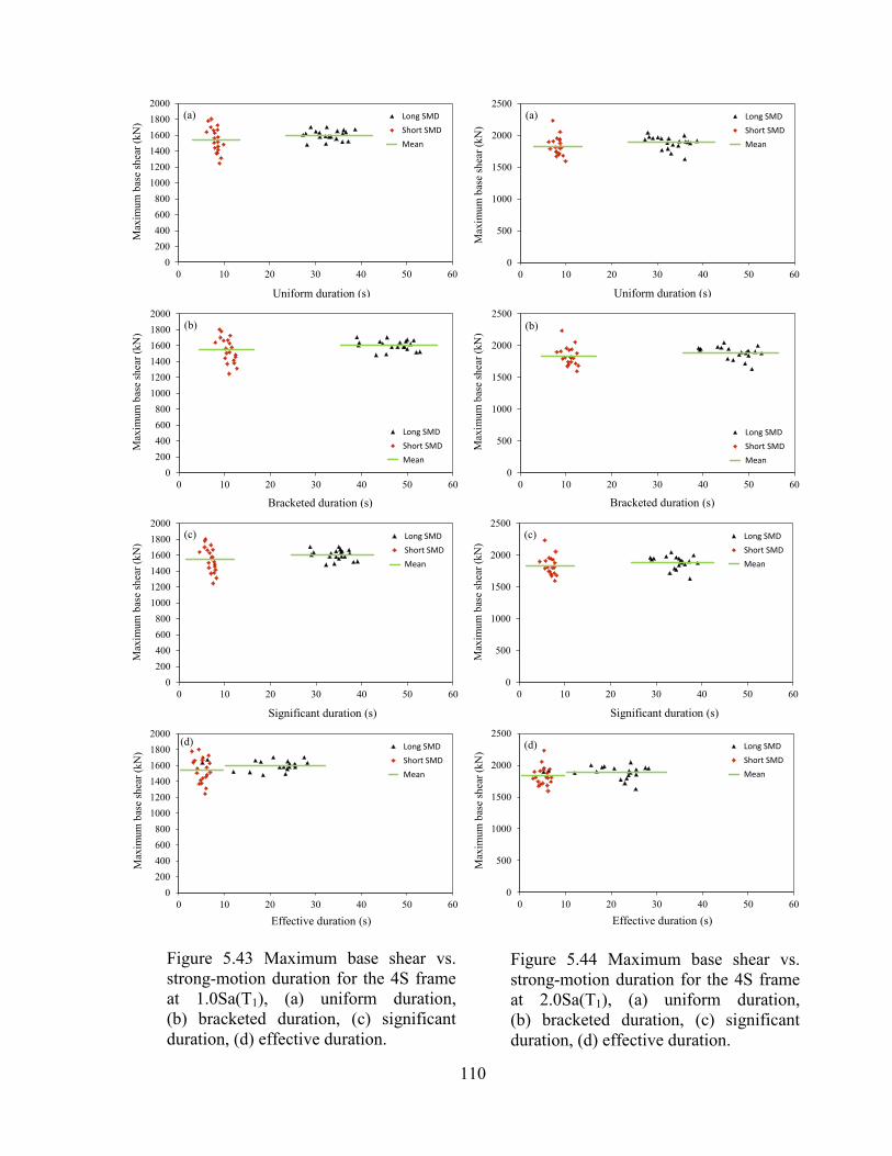
110
Uniform duration (s)
Bracketed duration (s)
Significant duration (s)
Effective duration (s)
Max
imum
bas
e sh
ear
(kN
) M
axim
um
bas
e sh
ear
(kN
) M
axim
um
bas
e sh
ear
(kN
) M
axim
um
bas
e sh
ear
(kN
)
Uniform duration (s)
Bracketed duration (s)
Significant duration (s)
Effective duration (s)
Max
imum
bas
e sh
ear
(kN
) M
axim
um
bas
e sh
ear
(kN
) M
axim
um
bas
e sh
ear
(kN
) M
axim
um
bas
e sh
ear
(kN
)
Figure 5.44 Maximum base shear vs.
strong-motion duration for the 4S frame
at 2.0Sa(T1), (a) uniform duration,
(b) bracketed duration, (c) significant
duration, (d) effective duration.
Figure 5.43 Maximum base shear vs.
strong-motion duration for the 4S frame
at 1.0Sa(T1), (a) uniform duration,
(b) bracketed duration, (c) significant
duration, (d) effective duration.
0
200
400
600
800
1000
1200
1400
1600
1800
2000
0 10 20 30 40 50 60
Long SMD
Short SMD
Mean
(a)
0
200
400
600
800
1000
1200
1400
1600
1800
2000
0 10 20 30 40 50 60
Long SMD
Short SMD
Mean
(b)
0
200
400
600
800
1000
1200
1400
1600
1800
2000
0 10 20 30 40 50 60
Long SMD
Short SMD
Mean
(c)
0
200
400
600
800
1000
1200
1400
1600
1800
2000
0 10 20 30 40 50 60
Long SMD
Short SMD
Mean
(d)
0
500
1000
1500
2000
2500
0 10 20 30 40 50 60
Long SMD
Short SMD
Mean
(a)
0
500
1000
1500
2000
2500
0 10 20 30 40 50 60
Long SMD
Short SMD
Mean
(b)
0
500
1000
1500
2000
2500
0 10 20 30 40 50 60
Long SMD
Short SMD
Mean
(c)
0
500
1000
1500
2000
2500
0 10 20 30 40 50 60
Long SMD
Short SMD
Mean
(d)

111
Uniform duration (s)
Bracketed duration (s)
Significant duration (s)
Effective duration (s)
Max
imum
bas
e sh
ear
(kN
) M
axim
um
bas
e sh
ear
(kN
) M
axim
um
bas
e sh
ear
(kN
) M
axim
um
bas
e sh
ear
(kN
)
Uniform duration (s)
Bracketed duration (s)
Significant duration (s)
Effective duration (s)
Figure 5.45 Maximum base shear vs.
strong-motion duration for the 10S frame
at 1.0Sa(T1), (a) uniform duration,
(b) bracketed duration, (c) significant
duration, (d) effective duration.
Figure 5.46 Maximum base shear vs.
strong-motion duration for the 10S frame
at 2.0Sa(T1), (a) uniform duration,
(b) bracketed duration, (c) significant
duration, (d) effective duration.
0
500
1000
1500
2000
2500
3000
3500
4000
0 10 20 30 40 50 60
Long SMD
Short SMD
Mean
(a)
0
500
1000
1500
2000
2500
3000
3500
4000
0 10 20 30 40 50 60
Long SMD
Short SMD
Mean
(b)
0
500
1000
1500
2000
2500
3000
3500
4000
0 10 20 30 40 50 60
Long SMD
Short SMD
Mean
(c)
0
500
1000
1500
2000
2500
3000
3500
4000
0 10 20 30 40 50 60
Long SMD
Short SMD
Mean
(d)
Max
imum
bas
e sh
ear
(kN
) M
axim
um
bas
e sh
ear
(kN
) M
axim
um
bas
e sh
ear
(kN
) M
axim
um
bas
e sh
ear
(kN
)
0
500
1000
1500
2000
2500
3000
3500
4000
4500
0 10 20 30 40 50 60
Long SMD
Short SMD
Mean
(a)
0
500
1000
1500
2000
2500
3000
3500
4000
4500
0 10 20 30 40 50 60
Long SMD
Short SMD
Mean
(b)
0
500
1000
1500
2000
2500
3000
3500
4000
4500
0 10 20 30 40 50 60
Long SMD
Short SMD
Mean
(c)
0
500
1000
1500
2000
2500
3000
3500
4000
4500
0 10 20 30 40 50 60
Long SMD
Short SMD
Mean
(d)

112
Uniform duration (s)
Bracketed duration (s)
Significant duration
(s)
Effective duration (s)
Max
imum
bas
e sh
ear
(kN
) M
axim
um
bas
e sh
ear
(kN
) M
axim
um
bas
e sh
ear
(kN
) M
axim
um
bas
e sh
ear
(kN
)
Uniform duration (s)
Bracketed duration (s)
Significant duration
(s)
Effective duration (s)
Max
imum
bas
e sh
ear
(kN
) M
axim
um
bas
e sh
ear
(kN
) M
axim
um
bas
e sh
ear
(kN
) M
axim
um
bas
e sh
ear
(kN
)
Figure 5.47 Maximum base shear vs.
strong-motion duration for the 16S frame
at 1.0Sa(T1), (a) uniform duration,
(b) bracketed duration, (c) significant
duration, (d) effective duration.
Figure 5.48 Maximum base shear vs.
strong-motion duration for the 16S frame
at 2.0Sa(T1), (a) uniform duration,
(b) bracketed duration, (c) significant
duration, (d) effective duration.
0
1000
2000
3000
4000
5000
6000
0 10 20 30 40 50 60
Long SMD
Short SMD
Mean
(a)
0
1000
2000
3000
4000
5000
6000
0 10 20 30 40 50 60
Long SMD
Short SMD
Mean
(b)
0
1000
2000
3000
4000
5000
6000
0 10 20 30 40 50 60
Long SMD
Short SMD
Mean
(c)
0
1000
2000
3000
4000
5000
6000
0 10 20 30 40 50 60
Long SMD
Short SMD
Mean
(d)
0
1000
2000
3000
4000
5000
6000
7000
8000
0 10 20 30 40 50 60
Long SMD
Short SMD
Mean
(a)
0
1000
2000
3000
4000
5000
6000
7000
8000
0 10 20 30 40 50 60
Long SMD
Short SMD
Mean
(b)
0
1000
2000
3000
4000
5000
6000
7000
8000
0 10 20 30 40 50 60
Long SMD
Short SMD
Mean
(c)
0
1000
2000
3000
4000
5000
6000
7000
8000
0 10 20 30 40 50 60
Long SMD
Short SMD
Mean
(d)

113
Chapter 6
Analysis Results from Real Records
6.1 Introduction
As mentioned in Chapter 3, two types of earthquake records are used for the
nonlinear time-history analysis in this study. One is the simulated records generated by
Atkinson (2009) representing the ground motions in Vancouver; the other is the real
records from earthquakes around the world. These two types of records are appropriate
for use for the time-history analysis as recommended by Lin et al. (2012). This section
will focus on the investigation of the effects of the strong-motion duration on the
structural response using real records. The seismic performance of the 4S, the 10S, and
the 16S frames based on the real records will not be discussed in this section. This is
because the preliminary study has showed that the performance of the three frames
assessed using the simulated records and the real records is very similar.
The results from the nonlinear time-history analysis of the 4S, the 10S and the
16S frames are shown in Figs. 6.1 to 6.30. Two intensity levels, i.e., 1.0Sa(T1) and
2.0Sa(T1), were considered in the analyses. The values of 1.0Sa(T1) and 2.0Sa(T1) for
each of the frames used to scale the records are given in Table 5.1 in Chapter 5. The short
SMD set and the long SMD set have 20 records each. Figures with designations of a, b,
and c are plotted with respect to the uniform duration, the bracketed duration and the
significant duration, respectively. It should be noted that the definition of the effective

114
duration is not considered in the plots. This is because the effective strong-motion
durations of many records in the set are less than 1 s, which are significantly smaller than
those determined according to the definitions of the uniform duration, the bracketed
duration and the significant duration. The response parameters considered in this section
include the interstorey drift (IDR), beam curvature ductility, column curvature ductility,
roof displacement, and base shear, which are the same parameters considered in the
analyses using simulated records (see the discussion in Chapter 5). Each point in the
figures in this section represents the maximum response of the frame from a given record
at a given excitation level.
6.2 Effects of Strong-motion Duration on the Structural Response
6.2.1 Interstorey drift
The maximum interstorey drift (IDR) vs. strong-motion duration for the 4S, the
10S and the 16S frames are presented in Figs. 6.1 to 6.6 in which Figs. 6.1 and 6.2 show
the results for the 4S frame at the excitation levels of 1.0Sa(T1) and 2.0Sa(T1),
respectively; Figs. 6.3 and 6.4 present the results for the 10S frame for each of the two
scaling levels mentioned above; and Figs. 6.5 and 6.6 show the results for the 16S frame.
Note that the IDR presented in the Figs. 6.1 to 6.6 are the largest IDR along the height of
the frame, i.e., it might occur at any floor depending on the record.
4S Frame
The results for the maximum IDR for the 4S frame from the short SMD set and
the long SMD set at the excitation levels of 1.0Sa(T1) and 2.0Sa(T1) are shown in Figs.

115
6.1 and 6.2, respectively. In general, the results for the 4S frame obtained from the real
records are very similar to those from the simulated record.
It is seen in Fig. 6.1 that at the excitation level of 1.0Sa(T1) the largest IDR from
the short SMD set is about 1.4% while from the long SMD set is about 2.0%. As
illustrated in Fig. 6.1, two records of the long SMD set produce relatively larger IDR than
any other records. The smallest IDRs from both sets are the same, which are about 0.7%.
The IDRs from the short SMD set have smaller dispersion than those from the long SMD
set. Regarding the mean value of IDR, the maximum mean IDR from the short SMD set
is about 1.0% and that from the long SMD set is about 1.1%, i.e., long SMD set gives
slightly larger IDR. It also can be seen in Fig. 6.1b that the data associated with the
bracketed duration are more spread than those with the uniform duration and the
significant duration. This is mainly because the definition of the bracketed duration gives
larger strong-motion duration than the definition of the uniform duration and significant
duration.
It can be seen in Fig. 6.2 that the largest IDR from the short SMD set is about
3.5%, while from the long SMD set is about 5.2% for the intensity of the excitation of
2.0Sa(T1). The smallest IDRs from the two sets are the same (around 1.1%). It is
necessary to mention that three records of the long SMD set provide extremely larger
IDR (i.e., more than 4%) compared to the other records, which is about 1% to 2%. In
general, the results obtained from the records scaled to 2.0Sa(T1) have very similar
features to those scaled to 1.0Sa(T1) in which the long SMD set provide larger IDR
(about 2.4%) than the short SMD set (about 1.9%), and the difference is about 30%. The
results for IDR obtained from the excitation levels of 1.0Sa(T1) and 2.0Sa(T1) show that
no regression function could be developed to correlate the IDR with the uniform strong-

116
motion duration, bracketed strong-motion duration, or the significant strong-motion
duration.
10S Frame
The results for the 10S frame at the excitation level of 1.0Sa(T1) are shown in Fig.
6.3. It can be seen in the figure that the short SMD set provides quite larger IDRs than the
long SMD set. This finding is consistent with that from the simulated records (Fig. 5.21).
More specifically, the maximum mean IDRs from the short and the long SMD sets are
about 1.6%, and 1.0%, respectively. The difference is about 60%, which is quite large
compared to that for the 4S frame. Considering the maximum IDR obtained from the
analyses, it is seen in the figure that it is between 1.0% and 2.5% from the short SMD set,
while it is between 0.8% and 1.4% from the long SMD set. It can be seen clearly in Fig
6.3 that the dispersion of the IDR from the short SMD set is much larger than that from
the long SMD set.
Comparing the results for IDR at the excitation level of 2.0Sa(T1) from the real
records (Fig. 6.4) to those from the simulated records (Fig. 5.22), it can be seen that the
maximum mean IDRs from the short SMD set of the real records and the simulated
records are very close, both are about 2.5%. However, the maximum mean IDR from the
long SMD set of the real records (about 1.9%) is smaller than that of the simulated
records (about 2.5%). The results in Fig. 6.4 clearly show that the short SMD set provides
larger IDR than the long SMD set when real records are used in the analysis. This
observation is different than that from the simulated records in which both the short and
the long SMD sets provide very similar IDRs for the 10S frame at the excitation level of

117
2.0Sa(T1). It indicates that the effect of the strong-motion duration on the structural
response depends on the type of the records used in the analysis.
16S Frame
The results for the 16S frame from the short SMD set and the long SMD set are
presented in Figs. 6.5 and 6.6, respectively. These results have similar feature to those for
the 10S frame. It can be seen in Fig. 6.5 that the short SMD set gives larger IDRs
compared to the long SMD set for the scaling level of 1.0Sa(T1). The IDRs from the short
SMD set are between 0.8% and 2.9%, while from the long SMD set they are between
0.8% and 1.9%. The maximum mean IDR from the short SMD set is about 1.7% while
from the long SMD set it is about 1.3%; the difference is about 30%. It is necessary to
mention that the mean IDRs obtained from the real records are larger than those from the
simulated records (Fig. 5.23, Chapter 5).
Regarding the results from the excitation level of 2.0Sa(T1), it can be seen in Fig.
6.6 that the IDR from the short SMD set ranges from 1.3% to 6.1%, and from the long
SMD set, it ranges from 1.6% to 3.0%. It is noticed that two records of the short SMD set
produce IDR larger than 5% which will cause the collapse of a building according to Lin
(2008). It is found that the maximum mean IDR from the short SMD set is about 3.2%
and that from the long SMD set is about 2.1%, the difference is about 50%. The results
for IDR for the 10S frame show that the maximum mean IDRs from the short and the
long SMD sets at the scaling level of 2.0Sa(T1) is almost twice and 1.5 times larger than
that at 1.0Sa(T1), respectively. Like for the 4S and 10S frames, there is no correlation
between the IDR and the strong-motion duration for the 16S frame in terms of all three
definitions of the strong-motion duration considered in the study.

118
6.2.2 Beam curvature ductility
The maximum beam curvature ductility vs. the strong-motion duration for the 4S,
the 10S and the 16S frames are plotted in Figs. 6.7 to 6.12. Figures 6.7 and 6.8 represent
the results for the 4S frame at the excitation levels of 1.0Sa(T1) and 2.0Sa(T1),
respectively. Figures 6.9 and 6.10 illustrate the results for the 10S frame for each of the
two scaling levels mentioned above. Figures 6.11 and 6.12 present the results for the 16S
frame. The detailed discussion on the results is given in the following sections.
4S Frame
The maximum beam curvature ductility for the 4S frame from the dynamic
analyses at the excitation level of 1.0Sa(T1) is shown in Fig. 6.7. As presented in the
figure, the smallest curvature ductilities generated from the records of the short and the
long SMD sets are almost the same, which are around 2.6. The largest curvature
ductilities from the two sets are different, the short SMD set gives about 5.5, and the long
SMD set gives about 7.1. Note that two records of the long SMD set produce relatively
larger ductility (> 6) than any other records of the short and the long SMD sets. The
maximum mean beam curvature ductilities from the two sets are the same, which are
about 3.9. This value is compatible with that obtained using the simulated records.
Moreover, the results in Fig. 6.7 clearly show that there is no correlation between the
beam curvature ductility and the strong-motion duration.
Similar to the results from the simulated records, the results from the real records
also show that the long SMD set gives larger curvature ductility compared to the short
SMD set for the 4S frame at the excitation level of 2.0Sa(T1). It is seen from Fig. 6.8 that

119
the maximum mean curvature ductility from the short SMD set is about 6.6, and from the
long SMD set it is about 8.0; the difference is about 20%. It is noticed that three records
of the long SMD set produce extremely large curvature ductility which is more than 13
compared to other records used in the analysis. Note that these three records also produce
quite large IDRs as discussed in Section 6.2.1. It is also found that the mean curvature
ductilities from the real records and those from the simulated records are close.
10S Frame
The results for the 10S frame corresponding to the scaling level of 1.0Sa(T1) are
shown in Fig. 6.9. It can be seen in the figure that the beam curvature ductilities from the
short SMD set are significantly larger than those from the long SMD set. The largest and
smallest curvature ductilities from the short SMD set are between 3.5 and 9.0, and from
the long SMD set they are between 2.9 and 5.9, they are compatible with those obtained
using simulated records. However the mean values from the real records and the
simulated records are different. The maximum mean beam curvature ductilities are about
6.3 and 4.3 from the short and the long SMD sets, respectively, and they are larger than
those from the simulated records, which are about 3.5.
Figure 6.10 shows the maximum beam curvature ductilities obtained from the
excitation level of 2.0Sa(T1). The results have similar features to those from the
excitation level of 1.0Sa(T1), i.e., the short SMD set provides extremely larger beam
curvature ductility than the long SMD set. A beam curvature ductility of about 9.7 was
obtained from the short SMD set, and about 6.9 from the long SMD set. They are about
1.5 times larger than those observed at the excitation level of 1.0Sa(T1). It indicates that
significant nonlinear deformations are occurred during the response at the excitation level

120
of 2.0Sa(T1). Based on the results shown in Figs. 6.9 and 6.10 it is concluded that no
correlation function could be developed between the beam curvature ductility and the
strong-motion duration.
16S Frame
The beam curvature ductilities for the 16S frame obtained at the excitation levels
of 1.0Sa(T1) and 2.0Sa(T1) are presented in Figs. 6.11 and 6.12, respectively. The
distribution of the results is very similar to that for the 10S frame. It can be seen in Fig.
6.11 that at the excitation level of 1.0Sa(T1) the smallest curvature ductilities from the
short and the long SMD sets are the same, which are about 3.1. However, the largest
curvature ductility from the two sets is different, i.e., the short SMD set gives the largest
curvature ductility of about 12.5 while the long SMD sets gives only about 6.7. In terms
of the mean value, the short SMD produces the maximum mean beam curvature ductility
of about 6.9, and the long SMD set about 4.9. These ductilities are very similar to those
of the 10S frame (Fig. 6.9). Like for the 10S frame, there is no mathematical function
that can be used to describe the relation between the beam curvature ductility and the
strong-motion duration in terms of uniform duration, bracketed duration, and significant
duration.
The results for the excitation level of 2.0Sa(T1) (Fig. 6.12) show that the short
SMD set gives larger curvature ductilities compared to the long SMD set. Comparing the
results with those obtained at 1.0Sa(T1), it can be seen that the curvature ductilities
associated with 2.0Sa(T1) are about 2 times larger than those associated with 1.0Sa(T1).
For example, the largest curvature ductilities from the short SMD set at the 1.0Sa(T1) and
2.0Sa(T1) are about 12.5 and 24.7, respectively. The maximum mean curvature ductility

121
from the short SMD set is about 13.3, and from the long SMD set is about 7.7. In general,
the results for the beam curvature ductility for the 16S frame show that the short SMD set
gives larger response than the long SMD set, and the difference is quite large, about 50%.
6.2.3 Column curvature ductility
The maximum column curvature ductilities resulting from the time-history
analyses for the three frames, the 4S, the 10S, and the 16S are shown in Figs. 6.13 to 6.18
in which Figs. 6.13 and 6.14 present the results for the 4S frame at 1.0Sa(T1) and
2.0Sa(T1), respectively; Figs. 6.15 and 6.16 present the results for the 10S frame, and
Figs. 6.17 and 6.18 present the results for the 16S frame.
4S Frame
The results for the column curvature ductility from the short SMD set and the
long SMD set at the scaling level of 1.0Sa(T1) shown in Fig. 6.13 indicate that both sets
of records give similar ductility. It can be seen in Fig. 6.13 that the largest column
curvature ductility is almost the same from both sets, in which it is about 2.8 from the
short SMD set and about 3.0 from the long SMD set. The calculation of the maximum
mean curvature ductility from the two sets shows that the short SMD set gives a mean
curvature ductility of about 1.7, while the long SMD set gives about 1.5 with a difference
around 15%. Comparing these results with the beam curvature ductilities (Fig. 6.7), it
was found that the beam curvature ductility is almost 2 to 3 times larger than the column
curvature ductility at 1.0Sa(T1) which is acceptable according to strong column-weak
beam criterion of the capacity design method.

122
In terms of the column curvature ductility at the scaling level of 2.0Sa(T1), the
results show that the column curvature ductility is about 2 times larger than that at
1.0Sa(T1). It can be seen in Fig. 6.14 that all the records give similar curvature ductility
between 1.2 and 4.0 except that one record of the short SMD set provides curvature
ductility of 5.0, and two records of the long SMD set provide curvature ductility up to
about 7.4. It is clear that larger dispersion is observed from the results at the excitation
level of 2.0Sa(T1) due to the nonlinearity of both beams and columns from different
records used in the analysis. Unlike the finding from the results at 1.0Sa(T1) in which the
short SMD set and the long SMD set give almost the same curvature ductility, at the
excitation level of 2.0Sa(T1) the long SMD sets gives relatively larger curvature ductility
than the short SMD set, the difference is about 14%. This observation is consistent with
that from the simulated records.
10S Frame
The maximum column curvature ductility for the 10S frame obtained from the
scaling level of 1.0Sa(T1) is shown in Fig. 6.15. The first observation of the results is that
the dispersion of the column curvature ductility from the short SMD set is much larger
than that from the long SMD set. This finding is the same as that from the simulated
records as given in Fig. 5.33. The smallest curvature ductilities from the two sets are
almost the same, which is about 1.0. However, the largest curvature ductility from the
short SMD set is about two times larger than that from the long SMD set. The second
observation is that the short SMD set gives larger maximum mean curvature ductility
than the long SMD set, i.e., the maximum mean curvature ductility from the short SMD
set is about 2.5 while from the long SMD set is about 1.3.

123
The results from the scaling level of 2.0Sa(T1) show that the short SMD set
provides larger column curvature ductility than the long SMD set. The range of the
curvature ductility from the short SMD set is between 1.7 and 5.0, while from the long
SMD set is between 1.0 and 3.2. The maximum mean column curvature ductilities are
about 3.3 and 2.1 from the short and the long SMD sets, respectively. These values are
increased about 30% compared to those obtained at the scaling level of 1.0Sa(T1).
The general conclusion from the results for the column curvature ductility for the
10S frame is that the short SMD set provides significant larger curvature ductility than
the long SMD set. In addition, the maximum mean curvature ductility from the long
SMD set from the real records is similar to that from the simulated records. However, the
mean curvature ductility from the short SMD set obtained using the real records is about
25% larger than that using the simulated records.
16S Frame
The results for the column curvature ductility for the 16S frame are shown in
Figs. 6.17 and 6.18 for the scaling levels of 1.0Sa(T1) and 2.0Sa(T1), respectively. These
results are similar to those for the 10S frame. For example, at 1.0Sa(T1) the mean column
curvature ductility for the 16S frame from the short SMD set is about 2.2, and for the 10S
frame it is about 2.5. The mean column curvature ductility for the 16S frame from the
long SMD set is about 1.5, while it is about 1.3 for the 10S frame. Generally, it is
expected that the response of the 16S frame is larger than that of the 10S frame since the
16S frame is more flexible than the 10S frame. The similar response of the 10S frame and
the 16S frame at the scaling level of 1.0Sa(T1) is mainly due to the fact that the
deformations occurred in the beams and columns are not significant, i.e., the behavior of

124
the beams and columns is at the earlier inelastic stage. The results in Fig. 6.17 show that
the short SMD set gives maximum mean column curvature ductility about 50% larger
than the long SMD set.
The results for the column curvature ductility for the 16S frame at the scaling
level of 2.0Sa(T1) have a similar feature to those at 1.0Sa(T1). The observations of the
results are, (1) the short SMD set produces larger curvature ductility than the long SMD
set. The maximum mean curvature ductility from the short SMD set is about 3.4, and
from the long SMD set is about 2.1; (2) the mean column curvature ductilities for the 16S
frame from both sets are the same as those for the 10S frame; (3) the mean curvature
ductilities for the 16S frame from the real records are about 40% larger than those from
the simulated records; (4) there is no correlation between the column curvature ductility
and any of the three definitions of the strong-motion duration considered in the study,
such as, uniform duration, bracketed duration, and significant duration.
6.2.4 Roof displacement
The roof displacement is another global response parameter, and it can be used to
assess the lateral stiffness of the frame when incorporated with the base shear force. The
results for the roof displacement for the 4S, the 10S and the 16S frames from the real
records for the excitation levels of 1.0Sa(T1) and 2.0Sa(T1) are shown in Figs. 6.19 to
6.20, 6.21 to 6.22, and 6.23 to 6.24, respectively.
4S Frame
Figure 6.19 shows the maximum roof displacement for the 4S frame from the
records scaled to 1.0Sa(T1). It is seen in the figure that the short SMD and the long SMD

125
sets produce the roof displacement in the same range of about 7 cm to 15 cm, except that
two records of the long SMD set give quite large values, one is about 18.7 cm and the
other is about 22 cm. It is worth mentioning that these two records also produce larger
IDR, beam curvature ductility, and column curvature ductility for the 4S frame at the
excitation level of 1.0Sa(T1) (Figs. 6.1, 6.7, and 6.13). The maximum mean roof
displacements from the short SMD and the long SMD sets are about 10 cm and 12 cm,
respectively, which indicates that the long SMD set gives slightly larger displacement
than the short SMD set. These mean values from the real records are close to those from
the simulated records (Fig. 5.37).
In terms of the maximum roof displacement at the excitation level of 2.0Sa(T1)
(Fig. 6.20), it can be seen that the maximum mean roof displacement from the short SMD
set is about 19 cm, and from the long SMD set is about 26 cm. Comparing these results
with those from the records scaled to 1.0Sa(T1), it is found that they are almost 2 times
larger than those obtained at 1.0Sa(T1). This is expected because the intensity of the
ground motion is doubled. It has also been noticed that the three records of the long SMD
set, which provide extremely large IDR, beam curvature ductility, and column curvature
ductility, also give quite large roof displacement in the order of 50 cm compared to other
records. The roof displacements obtained at the excitation level of 2.0Sa(T1) show that
the long SMD set provides larger responses than the short SMD set. In terms of the
correlation between the roof displacement and the strong-motion duration, no regression
function can be developed for the results obtained at both excitation levels considered in
the analyses.

126
10S Frame
An interesting observation of the maximum roof displacement for the 10S frame
from the scaling level of 1.0Sa(T1) (Fig. 6.21) is that the short and the long SMD sets
give very similar response. This was different than that for the 4S frame. The maximum
roof displacement from the short SMD set is in the range of 14 cm to 32 cm, and from the
long SMD set is in the range of 17 cm to 33 cm. The maximum mean roof displacements
from both sets of records are about 23 cm. Moreover, by examining the results for the
beam and column curvature ductilities at this scaling level, it can be seen that the
curvature ductility of the beam and column is not associated with the roof displacement.
For example, the mean roof displacements from the short SMD set and long SMD set are
almost the same at the scaling level 1.0Sa(T1) while the mean beam and column
ductilities from the short SMD set are significantly larger those from the long SMD (Figs.
6.9 and 6.15). As mentioned in Chapter 5, in general the roof displacement is considered
as a ''global'' response parameter, while the beam curvature ductility and column
curvature ductility are considered as a ''local'' response parameter.
The roof displacement from the scaling level of 2.0Sa(T1) (Fig. 6.22) shows a
similar distribution to that from the scaling level of 1.0Sa(T1). Both sets of the records
produce roof displacement between 26 cm and 55 cm except one record from the short
SMD set gives a displacement of about 74 cm and one record from the long SMD set
gives 64 cm. The maximum mean roof displacements from the two sets are the same,
which are about 40 cm. Like for other response parameters (IDR, beam curvature
ductility and column curvature ductility), no correlation was developed between the
maximum roof displacement and the uniform strong-motion duration (or bracketed

127
strong-motion duration, or the significant strong-motion duration) based on the results
shown in Figs. 6.21 and 6.22.
16S Frame
Figures 6.23 and 6.24 show the maximum roof displacements for the 16S frame
for the excitation levels of 1.0Sa(T1) and 2.0Sa(T1), respectively. The results show that
the maximum roof displacement for the 16S frame is larger than that for the 4S frame and
the 10S frame. It can be seen in Fig. 6.23 that the long SMD set provides larger roof
displacement than the short SMD set. More specifically, the maximum mean roof
displacement from the short SMD set is about 31 cm, and from the long SMD set is about
36 cm. The difference is about 10%. By comparing these mean values with those using
the simulated records, it is found that the real records and the simulated records produce
very similar mean displacements at the excitation level of 1.0Sa(T1). In addition, the
mean displacement of the 16S frame is about 1.5 times larger than that of the 10S frame,
3 times larger than that of the 4S frame for 1.0Sa(T1).
The results for the maximum roof displacement from the scaling level of
2.0Sa(T1) are given in Fig. 6.24. It is seen from the figure that the short and the long
SMD sets generate the same range of the displacement, i.e., between 40 cm and 90 cm
except two records of the short SMD set give relatively small displacement in the order
of 30 cm. In general, the maximum mean roof displacement from the long SMD set is
slightly larger than that from the short SMD set, the difference is about 5%.
Unlike the observation of the roof displacement for the excitation level of
1.0Sa(T1), it is found that the displacement obtained using the real records are much
smaller than that using the simulated records for the excitation level of 2.0Sa(T1). For

128
example, the largest displacement from the short SMD set of the real records is about 94
cm, while from the simulated records, is about 160 cm. This indicates that roof
displacement might not be considered as a “stable” global response parameter for a
certain type of structure since the response depends on the type of the records, i.e., real or
simulated. This is one of the reasons that current building codes use interstorey drift other
than roof displacement as a response parameter to limit the lateral displacement for the
design of buildings for seismic loads.
6.2.5 Base shear
It is known that base shear is used to represent the lateral load in the equivalent
static method for the design of building for seismic loads. As mentioned in the previous
section (i.e., section 5.2.4 and 5.2.5, base shear together with roof displacement can be
used to determine the global lateral stiffness of the frame in order to evaluate the stiffness
degradation of the frame during nonlinear response subjected to the seismic excitations.
4S Frame
The results for the maximum base shear for the 4S frame from the scaling levels
of 1.0Sa(T1) and 2.0Sa(T1) are presented in Figs. 6.25 and 6.26, respectively. It is seen in
Fig. 6.25 that the ranges of the maximum base shear from the short and the long SMD
sets are very similar for the level of 1.0Sa(T1), i.e., from both sets the base shear is
between 1300 kN and 1900 kN. Therefore, the dispersion of the response from the two
sets is identical. The results in Fig. 6.25 also show that the maximum mean base shear
forces from the short and the long SMD sets are almost the same, which are about 1600
kN.

129
The maximum base shear forces from the level of 2.0Sa(T1) (Fig. 6.26) show a
similar trend to those from the level of 1.0Sa(T1). The observations of the results are, (1)
the ranges of the base shear from the two sets are compatible, both are between 1600 kN
and 2200 kN; (2) the dispersion of the base shear obtained from the short and the long
SMD sets is almost the same; (3) the maximum mean base shear from the two sets are
very close, which are about 1900 kN; (4) the mean base shear for the excitations scaled to
2.0Sa(T1) is increased about 20% compared to that for the excitations scaled to 1.0Sa(T1).
Based on the results shown in Figs. 6.25 and 6.26, it is concluded that there is no
correlation between the base shear and the strong-motion duration regardless of the
definitions of the strong-motion duration considered, such as, uniform duration,
bracketed duration, or significant duration.
It is worth mentioning that the mean base shear forces from the real records for
the excitations scaled to 1.0Sa(T1) and 2.0Sa(T1) are very similar to those from the
simulated records. It indicates that the base shear may not depend on the type of the
records used in the time-history analysis for structures with short period, however further
research is needed in order to confirm this conclusion.
10S Frame
Unlike the results for the 4S frame, the observations of the results for the 10S
frame (Figs. 6.27 and 6.28) show that the short SMD set gives significantly larger base
shear than the long SMD set. At the scaling level of 1.0Sa(T1), the maximum mean base
shear from the short SMD set is about 3400 kN, and from the long SMD set is about 2300
kN. The difference is about 50%. At the scaling level of 2.0Sa(T1), the maximum mean
base shear from the short SMD set is about 4200 kN, and from the long SMD set is about

130
2800 kN. The difference is also about 50%. Overall the base shear is increased about
20% from the excitation level of 1.0Sa(T1) to 2.0Sa(T1). The base shear forces from the
real records are also compared to those from the simulated records. It is found that the
mean base shear from the real records is about 20% larger than that from the simulated
records.
16S Frame
The maximum base shear forces for the 16S frame from the analyses associated
with the records scaled to 1.0Sa(T1) and 2.0Sa(T1) are shown in Figs. 6.29 and 6.30,
respectively. The observation of the results for the 16S frame is the same as that of the
10S frame, i.e., the short SMD set produces significantly larger base shear force than the
long SMD set. The difference between the two sets is extremely larger for the 16S frame
compared to that for the 4S and 10S frames, which is about 60% to 80%. For example,
for the scaling level of 1.0Sa(T1) the maximum mean base shear from the short SMD set
is about 5500 kN, and from the long SMD set is about 3100 kN, so the difference is about
80%. It indicates that significant inelastic deformations are occurred in the beams and
columns of the 16S frame during the response at the excitation level of 1.0Sa(T1). Similar
to the findings from the results for the 10S frame, it is found that the base shear forces for
the 16S frame from the real records are extremely larger than those from the simulated
records (about 40%) except the shear force from the long SMD set obtained at the scaling
level of 1.0Sa(T1) in which the difference is only about 5%. Like for the 4S frame and the
10S frame, regression correlation function could not be developed between the base shear
and the strong-motion duration.

131
Figure 6.2 Maximum interstorey drift vs.
strong-motion duration for the 4S frame
at 2.0Sa(T1), (a) uniform duration,
(b) bracketed duration, (c) significant
duration.
Figure 6.1 Maximum interstorey drift vs.
strong-motion duration for the 4S frame
at 1.0Sa(T1), (a) uniform duration,
(b) bracketed duration, (c) significant
duration.
0
0.5
1
1.5
2
2.5
0 20 40 60 80
Long SMD
Short SMD
Mean
(a)
0
0.5
1
1.5
2
2.5
0 20 40 60 80
Long SMD
Short SMD
Mean
(b)
0
0.5
1
1.5
2
2.5
0 20 40 60 80
Long SMD
Short SMD
Mean
(c)
0
1
2
3
4
5
6
0 20 40 60 80
Long SMD
Short SMD
Mean
(a)
0
1
2
3
4
5
6
0 20 40 60 80
Long SMD
Short SMD
Mean
(b)
0
1
2
3
4
5
6
0 20 40 60 80
Long SMD
Short SMD
Mean
(c)
Max
imum
inte
rsto
rey
dri
ft (
%)
Max
imum
inte
rsto
rey
dri
ft (
%)
Max
imum
inte
rsto
rey
dri
ft (
%)
Uniform duration (s)
Bracketed duration (s)
Significant duration (s)
Max
imum
inte
rsto
rey
dri
ft (
%)
Max
imum
inte
rsto
rey
dri
ft (
%)
Max
imum
inte
rsto
rey
dri
ft (
%)
Uniform duration (s)
Bracketed duration (s)
Significant duration (s)

132
Figure 6.3 Maximum interstorey drift vs.
strong-motion duration for the 10S frame
at 1.0Sa(T1), (a) uniform duration,
(b) bracketed duration, (c) significant
duration.
Figure 6.4 Maximum interstorey drift vs.
strong-motion duration for the 10S frame
at 2.0Sa(T1), (a) uniform duration,
(b) bracketed duration, (c) significant
duration.
0
0.5
1
1.5
2
2.5
3
0 20 40 60 80
Long SMD
Short SMD
Mean
(a)
0
0.5
1
1.5
2
2.5
3
0 20 40 60 80
Long SMD
Short SMD
Mean
(b)
0
0.5
1
1.5
2
2.5
3
0 20 40 60 80
Long SMD
Short SMD
Mean
(c)
0
0.5
1
1.5
2
2.5
3
3.5
4
0 20 40 60 80
Long SMD
Short SMD
Mean
(a)
0
0.5
1
1.5
2
2.5
3
3.5
4
0 20 40 60 80
Long SMD
Short SMD
Mean
(b)
0
0.5
1
1.5
2
2.5
3
3.5
4
0 20 40 60 80
Long SMD
Short SMD
Mean
(c)
Max
imum
inte
rsto
rey
dri
ft (
%)
Max
imum
inte
rsto
rey
dri
ft (
%)
Max
imum
inte
rsto
rey
dri
ft (
%)
Uniform duration (s)
Bracketed duration (s)
Significant duration (s)
Max
imum
inte
rsto
rey
dri
ft (
%)
Max
imum
inte
rsto
rey
dri
ft (
%)
Max
imum
inte
rsto
rey
dri
ft (
%)
Uniform duration (s)
Bracketed duration (s)
Significant duration (s)

133
Figure 6.5 Maximum interstorey drift vs.
strong-motion duration for the 16S frame
at 1.0Sa(T1), (a) uniform duration,
(b) bracketed duration, (c) significant
duration.
Figure 6.6 Maximum interstorey drift vs.
strong-motion duration for the 16S frame
at 2.0Sa(T1), (a) uniform duration,
(b) bracketed duration, (c) significant
duration.
0
0.5
1
1.5
2
2.5
3
3.5
0 20 40 60 80
Long SMD
Short SMD
Mean
(a)
0
0.5
1
1.5
2
2.5
3
3.5
0 20 40 60 80
Long SMD
Short SMD
Mean
(b)
0
0.5
1
1.5
2
2.5
3
3.5
0 20 40 60 80
Long SMD
Short SMD
Mean
(c)
0
1
2
3
4
5
6
7
0 20 40 60 80
Long SMD
Short SMD
Mean
(a)
0
1
2
3
4
5
6
7
0 20 40 60 80
Long SMD
Short SMD
Mean
(b)
0
1
2
3
4
5
6
7
0 20 40 60 80
Long SMD
Short SMD
Mean
(c)
Max
imum
inte
rsto
rey
dri
ft (
%)
Max
imum
inte
rsto
rey
dri
ft (
%)
Max
imum
inte
rsto
rey
dri
ft (
%)
Uniform duration (s)
Bracketed duration (s)
Significant duration (s)
Max
imum
inte
rsto
rey
dri
ft (
%)
Max
imum
inte
rsto
rey
dri
ft (
%)
Max
imum
inte
rsto
rey
dri
ft (
%)
Uniform duration (s)
Bracketed duration (s)
Significant duration (s)

134
Figure 6.7 Maximum beam curvature
ductility vs. strong-motion duration for
the 4S frame at 1.0Sa(T1), (a) uniform
duration, (b) bracketed duration, (c)
significant duration.
Figure 6.8 Maximum beam curvature
ductility vs. strong-motion duration for
the 4S frame at 2.0Sa(T1), (a) uniform
duration, (b) bracketed duration, (c)
significant duration.
Max
imum
bea
m c
urv
atu
re d
uct
ilit
y
0
1
2
3
4
5
6
7
8
0 20 40 60 80
Long SMD
Short SMD
Mean
(a)
0
1
2
3
4
5
6
7
8
0 20 40 60 80
Long SMD
Short SMD
Mean
(b)
0
1
2
3
4
5
6
7
8
0 20 40 60 80
Long SMD
Short SMD
Mean
(c)
0
2
4
6
8
10
12
14
16
18
0 20 40 60 80
Long SMD
Short SMD
Mean
(a)
0
2
4
6
8
10
12
14
16
18
0 20 40 60 80
Long SMD
Short SMD
Mean
(b)
0
2
4
6
8
10
12
14
16
18
0 20 40 60 80
Long SMD
Short SMD
Mean
(c)
Max
imum
bea
m c
urv
atu
re d
uct
ilit
y
Max
imum
bea
m c
urv
atu
re d
uct
ilit
y
Max
imum
bea
m c
urv
atu
re d
uct
ilit
y
Uniform duration (s)
Bracketed duration (s)
Significant duration (s)
Max
imum
bea
m c
urv
atu
re d
uct
ilit
y
Max
imum
bea
m c
urv
atu
re d
uct
ilit
y
Max
imum
bea
m c
urv
atu
re d
uct
ilit
y
Uniform duration (s)
Bracketed duration (s)
Significant duration (s)

135
Figure 6.9 Maximum beam curvature
ductility vs. strong-motion duration for
the 10S frame at 1.0Sa(T1), (a) uniform
duration, (b) bracketed duration, (c)
significant duration.
Figure 6.10 Maximum beam curvature
ductility vs. strong-motion duration for
the 10S frame at 2.0Sa(T1), (a) uniform
duration, (b) bracketed duration, (c)
significant duration.
0
1
2
3
4
5
6
7
8
9
10
0 20 40 60 80
Long SMD
Short SMD
Mean
(a)
0
1
2
3
4
5
6
7
8
9
10
0 20 40 60 80
Long SMD
Short SMD
Mean
(b)
0
1
2
3
4
5
6
7
8
9
10
0 20 40 60 80
Long SMD
Short SMD
Mean
(c)
0
2
4
6
8
10
12
14
0 20 40 60 80
Long SMD
Short SMD
Mean
(a)
0
2
4
6
8
10
12
14
0 20 40 60 80
Long SMD
Short SMD
Mean
(b)
0
2
4
6
8
10
12
14
0 20 40 60 80
Long SMD
Short SMD
Mean
(c)
Max
imum
bea
m c
urv
atu
re d
uct
ilit
y
Max
imum
bea
m c
urv
atu
re d
uct
ilit
y
Max
imum
bea
m c
urv
atu
re d
uct
ilit
y
Uniform duration (s)
Bracketed duration (s)
Significant duration (s)
Max
imum
bea
m c
urv
atu
re d
uct
ilit
y
Max
imum
bea
m c
urv
atu
re d
uct
ilit
y
Max
imum
bea
m c
urv
atu
re d
uct
ilit
y
Uniform duration (s)
Bracketed duration (s)
Significant duration (s)

136
Figure 6.11 Maximum beam curvature
ductility vs. strong-motion duration for
the 16S frame at 1.0Sa(T1), (a) uniform
duration, (b) bracketed duration, (c)
significant duration.
Figure 6.12 Maximum beam curvature
ductility vs. strong-motion duration for
the 16S frame at 2.0Sa(T1), (a) uniform
duration, (b) bracketed duration, (c)
significant duration.
0
2
4
6
8
10
12
14
0 20 40 60 80
Long SMD
Short SMD
Mean
(a)
0
2
4
6
8
10
12
14
0 20 40 60 80
Long SMD
Short SMD
Mean
(b)
0
2
4
6
8
10
12
14
0 20 40 60 80
Long SMD
Short SMD
Mean
(c)
0
5
10
15
20
25
30
0 20 40 60 80
Long SMD
Short SMD
Mean
(a)
0
5
10
15
20
25
30
0 20 40 60 80
Long SMD
Short SMD
Mean
(b)
0
5
10
15
20
25
30
0 20 40 60 80
Long SMD
Short SMD
Mean
(c)
Max
imum
bea
m c
urv
atu
re d
uct
ilit
y
Max
imum
bea
m c
urv
atu
re d
uct
ilit
y
Max
imum
bea
m c
urv
atu
re d
uct
ilit
y
Uniform duration (s)
Bracketed duration (s)
Significant duration (s)
Max
imum
bea
m c
urv
atu
re d
uct
ilit
y
Max
imum
bea
m c
urv
atu
re d
uct
ilit
y
Max
imum
bea
m c
urv
atu
re d
uct
ilit
y
Uniform duration (s)
Bracketed duration (s)
Significant duration (s)

137
Figure 6.14 Maximum column curvature
ductility vs. strong-motion duration for
the 4S frame at 2.0Sa(T1), (a) uniform
duration, (b) bracketed duration, (c)
significant duration.
Figure 6.13 Maximum column curvature
ductility vs. strong-motion duration for
the 4S frame at 1.0Sa(T1), (a) uniform
duration, (b) bracketed duration, (c)
significant duration.
Max
imum
colu
mn c
urv
ature
du
ctil
ity
Max
imum
colu
mn c
urv
ature
du
ctil
ity
M
axim
um
colu
mn c
urv
ature
du
ctil
ity
0
0.5
1
1.5
2
2.5
3
3.5
0 20 40 60 80
Long SMD
Short SMD
Mean
(a)
0
0.5
1
1.5
2
2.5
3
3.5
0 20 40 60 80
Long SMD
Short SMD
Mean
(b)
0
0.5
1
1.5
2
2.5
3
3.5
0 20 40 60 80
Long SMD
Short SMD
Mean
(c)
0
1
2
3
4
5
6
7
8
0 20 40 60 80
Long SMD
Short SMD
Mean
(a)
0
1
2
3
4
5
6
7
8
0 20 40 60 80
Long SMD
Short SMD
Mean
(b)
0
1
2
3
4
5
6
7
8
0 20 40 60 80
Long SMD
Short SMD
Mean
(c)
Uniform duration (s)
Bracketed duration (s)
Significant duration (s)
Max
imum
colu
mn c
urv
ature
du
ctil
ity
Max
imum
colu
mn c
urv
ature
du
ctil
ity
M
axim
um
colu
mn c
urv
ature
du
ctil
ity
Uniform duration (s)
Bracketed duration (s)
Significant duration (s)

138
Figure 6.15 Maximum column curvature
ductility vs. strong-motion duration for
the 10S frame at 1.0Sa(T1), (a) uniform
duration, (b) bracketed duration, (c)
significant duration.
Figure 6.16 Maximum column curvature
ductility vs. strong-motion duration for
the 10S frame at 2.0Sa(T1), (a) uniform
duration, (b) bracketed duration, (c)
significant duration.
0
0.5
1
1.5
2
2.5
3
3.5
4
0 20 40 60 80
Long SMD
Short SMD
Mean
(a)
0
0.5
1
1.5
2
2.5
3
3.5
4
0 20 40 60 80
Long SMD
Short SMD
Mean
(b)
0
0.5
1
1.5
2
2.5
3
3.5
4
0 20 40 60 80
Long SMD
Short SMD
Mean
(c)
0
1
2
3
4
5
6
0 20 40 60 80
Long SMD
Short SMD
Mean
(a)
0
1
2
3
4
5
6
0 20 40 60 80
Long SMD
Short SMD
Mean
(b)
0
1
2
3
4
5
6
0 20 40 60 80
Long SMD
Short SMD
Mean
(c)
Max
imum
colu
mn c
urv
ature
du
ctil
ity
Max
imum
colu
mn c
urv
ature
du
ctil
ity
M
axim
um
colu
mn c
urv
ature
du
ctil
ity
Uniform duration (s)
Bracketed duration (s)
Significant duration (s)
Max
imum
colu
mn c
urv
ature
du
ctil
ity
Max
imum
colu
mn c
urv
ature
du
ctil
ity
M
axim
um
colu
mn c
urv
ature
du
ctil
ity
Uniform duration (s)
Bracketed duration (s)
Significant duration (s)

139
Figure 6.18 Maximum column curvature
ductility vs. strong-motion duration for
the 16S frame at 2.0Sa(T1), (a) uniform
duration, (b) bracketed duration, (c)
significant duration.
Figure 6.17 Maximum column curvature
ductility vs. strong-motion duration for
the 16S frame at 1.0Sa(T1), (a) uniform
duration, (b) bracketed duration, (c)
significant duration.
0
0.5
1
1.5
2
2.5
3
3.5
4
0 20 40 60 80
Long SMD
Short SMD
Mean
(a)
0
0.5
1
1.5
2
2.5
3
3.5
4
0 20 40 60 80
Long SMD
Short SMD
Mean
(b)
0
0.5
1
1.5
2
2.5
3
3.5
4
0 20 40 60 80
Long SMD
Short SMD
Mean
(c)
0
1
2
3
4
5
6
7
8
0 20 40 60 80
Long SMD
Short SMD
Mean
(a)
0
1
2
3
4
5
6
7
8
0 20 40 60 80
Long SMD
Short SMD
Mean
(b)
0
1
2
3
4
5
6
7
8
0 20 40 60 80
Long SMD
Short SMD
Mean
(c)
Max
imum
colu
mn c
urv
ature
du
ctil
ity
Max
imum
colu
mn c
urv
ature
du
ctil
ity
M
axim
um
colu
mn c
urv
ature
du
ctil
ity
Uniform duration (s)
Bracketed duration (s)
Significant duration (s)
Max
imum
colu
mn c
urv
ature
du
ctil
ity
Max
imum
colu
mn c
urv
ature
du
ctil
ity
M
axim
um
colu
mn c
urv
ature
du
ctil
ity
Uniform duration (s)
Bracketed duration (s)
Significant duration (s)

140
Figure 6.20 Maximum roof displacement
vs. strong-motion duration for the 4S
frame at 2.0Sa(T1), (a) uniform duration,
(b) bracketed duration, (c) significant
duration.
Figure 6.19 Maximum roof displacement
vs. strong-motion duration for the 4S
frame at 1.0Sa(T1), (a) uniform duration,
(b) bracketed duration, (c) significant
duration.
0
5
10
15
20
25
0 10 20 30 40 50 60 70 80
Long SMD
Short SMD
Mean
(a)
0
5
10
15
20
25
0 10 20 30 40 50 60 70 80
Long SMD
Short SMD
Mean
(b)
0
5
10
15
20
25
0 10 20 30 40 50 60 70 80
Long SMD
Short SMD
Mean
(c)
0
10
20
30
40
50
60
0 10 20 30 40 50 60 70 80
Long SMD
Short SMD
Mean
(a)
0
10
20
30
40
50
60
0 10 20 30 40 50 60 70 80
Long SMD
Short SMD
Mean
(b)
0
10
20
30
40
50
60
0 10 20 30 40 50 60 70 80
Long SMD
Short SMD
Mean
(c)
Max
imum
roo
f dis
pla
cem
ent
(cm
) M
axim
um
roo
f dis
pla
cem
ent
(cm
) M
axim
um
roo
f dis
pla
cem
ent
(cm
)
Uniform duration (s)
Bracketed duration (s)
Significant duration (s)
Max
imum
roo
f dis
pla
cem
ent
(cm
) M
axim
um
roo
f dis
pla
cem
ent
(cm
) M
axim
um
roo
f dis
pla
cem
ent
(cm
)
Uniform duration (s)
Bracketed duration (s)
Significant duration (s)

141
Figure 6.22 Maximum roof displacement
vs. strong-motion duration for the 10S
frame at 2.0Sa(T1), (a) uniform duration,
(b) bracketed duration, (c) significant
duration.
Figure 6.21 Maximum roof displacement
vs. strong-motion duration for the 10S
frame at 1.0Sa(T1), (a) uniform duration,
(b) bracketed duration, (c) significant
duration.
0
5
10
15
20
25
30
35
0 10 20 30 40 50 60 70 80
Long SMD
Short SMD
Mean
(a)
0
5
10
15
20
25
30
35
0 10 20 30 40 50 60 70 80
Long SMD
Short SMD
Mean
(b)
0
5
10
15
20
25
30
35
0 10 20 30 40 50 60 70 80
Long SMD
Short SMD
Mean
(c)
0
10
20
30
40
50
60
70
80
0 10 20 30 40 50 60 70 80
Long SMD
Short SMD
Mean
(a)
0
10
20
30
40
50
60
70
80
0 10 20 30 40 50 60 70 80
Long SMD
Short SMD
Mean
(b)
0
10
20
30
40
50
60
70
80
0 10 20 30 40 50 60 70 80
Long SMD
Short SMD
Mean
(c)
Max
imum
roo
f dis
pla
cem
ent
(cm
) M
axim
um
roo
f dis
pla
cem
ent
(cm
) M
axim
um
roo
f dis
pla
cem
ent
(cm
)
Uniform duration (s)
Bracketed duration (s)
Significant duration (s)
Max
imum
roo
f dis
pla
cem
ent
(cm
) M
axim
um
roo
f dis
pla
cem
ent
(cm
) M
axim
um
roo
f dis
pla
cem
ent
(cm
)
Uniform duration (s)
Bracketed duration (s)
Significant duration (s)

142
Figure 6.24 Maximum roof displacement
vs. strong-motion duration for the 16S
frame at 2.0Sa(T1), (a) uniform duration,
(b) bracketed duration, (c) significant
duration.
Figure 6.23 Maximum roof displacement
vs. strong-motion duration for the 16S
frame at 1.0Sa(T1), (a) uniform duration,
(b) bracketed duration, (c) significant
duration.
0
5
10
15
20
25
30
35
40
45
50
0 10 20 30 40 50 60 70 80
Long SMD
Short SMD
Mean
(a)
0
5
10
15
20
25
30
35
40
45
50
0 10 20 30 40 50 60 70 80
Long SMD
Short SMD
Mean
(b)
0
5
10
15
20
25
30
35
40
45
50
0 10 20 30 40 50 60 70 80
Long SMD
Short SMD
Mean
(c)
0
10
20
30
40
50
60
70
80
90
100
0 10 20 30 40 50 60 70 80
Long SMD
Short SMD
Mean
(a)
0
10
20
30
40
50
60
70
80
90
100
0 10 20 30 40 50 60 70 80
Long SMD
Short SMD
Mean
(b)
0
10
20
30
40
50
60
70
80
90
100
0 10 20 30 40 50 60 70 80
Long SMD
Short SMD
Mean
(c)
Max
imum
roo
f dis
pla
cem
ent
(cm
) M
axim
um
roo
f dis
pla
cem
ent
(cm
) M
axim
um
roo
f dis
pla
cem
ent
(cm
)
Uniform duration (s)
Bracketed duration (s)
Significant duration (s)
Max
imum
roo
f dis
pla
cem
ent
(cm
) M
axim
um
roo
f dis
pla
cem
ent
(cm
) M
axim
um
roo
f dis
pla
cem
ent
(cm
)
Uniform duration (s)
Bracketed duration (s)
Significant duration (s)

143
Figure 6.26 Maximum base shear vs.
strong-motion duration for the 4S frame
at 2.0Sa(T1), (a) uniform duration,
(b) bracketed duration, (c) significant
duration.
Figure 6.25 Maximum base shear vs.
strong-motion duration for the 4S frame
at 1.0Sa(T1), (a) uniform duration,
(b) bracketed duration, (c) significant
duration.
0
500
1000
1500
2000
2500
0 10 20 30 40 50 60 70 80
Long SMD
Short SMD
Mean
(a)
0
500
1000
1500
2000
2500
0 10 20 30 40 50 60 70 80
Long SMD
Short SMD
Mean
(b)
0
500
1000
1500
2000
2500
0 10 20 30 40 50 60 70 80
Long SMD
Short SMD
Mean
(c)
0
500
1000
1500
2000
2500
0 10 20 30 40 50 60 70 80
Long SMD
Short SMD
Mean
(a)
0
500
1000
1500
2000
2500
0 10 20 30 40 50 60 70 80
Long SMD
Short SMD
Mean
(b)
0
500
1000
1500
2000
2500
0 10 20 30 40 50 60 70 80
Long SMD
Short SMD
Mean
(c)
Max
imum
bas
e sh
ear
(kN
) M
axim
um
bas
e sh
ear
(kN
) M
axim
um
bas
e sh
ear
(kN
)
Uniform duration (s)
Bracketed duration (s)
Significant duration (s)
Max
imum
bas
e sh
ear
(kN
) M
axim
um
bas
e sh
ear
(kN
) M
axim
um
bas
e sh
ear
(kN
)
Uniform duration (s)
Bracketed duration (s)
Significant duration (s)

144
Figure 6.28 Maximum base shear vs.
strong-motion duration for the 10S frame
at 2.0Sa(T1), (a) uniform duration,
(b) bracketed duration, (c) significant
duration.
Figure 6.27 Maximum base shear vs.
strong-motion duration for the 10S frame
at 1.0Sa(T1), (a) uniform duration,
(b) bracketed duration, (c) significant
duration.
0
500
1000
1500
2000
2500
3000
3500
4000
4500
5000
0 10 20 30 40 50 60 70 80
Long SMD
Short SMD
Mean
(a)
0
500
1000
1500
2000
2500
3000
3500
4000
4500
5000
0 10 20 30 40 50 60 70 80
Long SMD
Short SMD
Mean
(b)
0
500
1000
1500
2000
2500
3000
3500
4000
4500
5000
0 10 20 30 40 50 60 70 80
Long SMD
Short SMD
Mean
(c)
0
1000
2000
3000
4000
5000
6000
0 10 20 30 40 50 60 70 80
Long SMD
Short SMD
Mean
(a)
0
1000
2000
3000
4000
5000
6000
0 10 20 30 40 50 60 70 80
Long SMD
Short SMD
Mean
(b)
0
1000
2000
3000
4000
5000
6000
0 10 20 30 40 50 60 70 80
Long SMD
Short SMD
Mean
(c)
Max
imum
bas
e sh
ear
(kN
) M
axim
um
bas
e sh
ear
(kN
) M
axim
um
bas
e sh
ear
(kN
)
Uniform duration (s)
Bracketed duration (s)
Significant duration (s)
Max
imum
bas
e sh
ear
(kN
) M
axim
um
bas
e sh
ear
(kN
) M
axim
um
bas
e sh
ear
(kN
)
Uniform duration (s)
Bracketed duration (s)
Significant duration (s)

145
Figure 6.30 Maximum base shear vs.
strong-motion duration for the 16S frame
at 2.0Sa(T1), (a) uniform duration,
(b) bracketed duration, (c) significant
duration.
Figure 6.29 Maximum base shear vs.
strong-motion duration for the 16S frame
at 1.0Sa(T1), (a) uniform duration,
(b) bracketed duration, (c) significant
duration.
0
1000
2000
3000
4000
5000
6000
7000
8000
9000
10000
0 10 20 30 40 50 60 70 80
Long SMD
Short SMD
Mean
(a)
0
1000
2000
3000
4000
5000
6000
7000
8000
9000
10000
0 10 20 30 40 50 60 70 80
Long SMD
Short SMD
Mean
(b)
0
1000
2000
3000
4000
5000
6000
7000
8000
9000
10000
0 10 20 30 40 50 60 70 80
Long SMD
Short SMD
Mean
(c)
0
2000
4000
6000
8000
10000
12000
0 10 20 30 40 50 60 70 80
Long SMD
Short SMD
Mean
(a)
0
2000
4000
6000
8000
10000
12000
0 10 20 30 40 50 60 70 80
Long SMD
Short SMD
Mean
(b)
0
2000
4000
6000
8000
10000
12000
0 10 20 30 40 50 60 70 80
Long SMD
Short SMD
Mean
(c)
Max
imum
bas
e sh
ear
(kN
) M
axim
um
bas
e sh
ear
(kN
) M
axim
um
bas
e sh
ear
(kN
)
Uniform duration (s)
Bracketed duration (s)
Significant duration (s)
Max
imum
bas
e sh
ear
(kN
) M
axim
um
bas
e sh
ear
(kN
) M
axim
um
bas
e sh
ear
(kN
)
Uniform duration (s)
Bracketed duration (s)
Significant duration (s)

146
Chapter 7
Discussion and Conclusions
7.1 Discussion
The strong portion of an earthquake record at a given site is normally referred to
as the strong-motion duration. Several parameters affect the strong-motion duration
including the earthquake magnitude, the distance from the earthquake source to the site
where the record is obtained, the soil condition at the site, the type of the earthquake, etc.
A number of studies have been conducted on the investigation of the effects of the
strong-motion duration on the structural response/structural damage. However the
conclusions from these studies are very contradictory. Some studies report significant
effects while others report minimal or no effects. Therefore, there is a need for further
investigations into the strong-motion duration of an earthquake record. The major
objective of this thesis is to investigate the effects of the strong-motion duration on the
seismic response of reinforced concrete frame buildings and the correlation between the
structural response and the strong-motion duration of earthquake records.
For the purpose of this study, three reinforced concrete frame (4-, 10-, and 16-
storey) buildings located in Vancouver were used in the analysis. The buildings were
designed according to the 2005 edition of the National Building Code of Canada
(NBCC). The 4-storey, the 10-storey, and the 16-storey buildings considered in this study
were used to represent the behaviour of the low-rise, the medium-rise, and the high-rise

147
buildings, respectively. Nonlinear time-history analyses were conducted by subjecting
each of the three frames to the selected sets of accelerograms representative for the
Vancouver region. Each set of the records was scaled to three excitation levels, i.e.,
0.5Sa(T1), 1.0Sa(T1), and 2.0Sa(T1) in which T1 represents the fundamental period of the
frame. The value of Sa(T1) was determined based on the design spectrum for Vancouver
for the probability of exceedance of 2% in 50 years. These excitation levels were selected
in order to cover a range of the frame response from elastic to inelastic.
The definitions of strong-motion duration considered in this study were uniform
duration, bracketed duration, significant duration and effective duration. Uniform
duration is defined as the sum of the time intervals in which acceleration exceeds a
specific threshold. Bracketed duration is defined as the total time elapsed between the
first and last excursion of a specified level of acceleration. Significant strong-motion
duration is an energy-based definition, and it represents the portion of a record where
90% of the total energy is accumulated. According to the definition of effective duration,
the start time of the strong motion is considered as the time when the energy in a record is
equal to 0.01 m/s, while the end time is considered as the time when the remaining
energy in the record is equal to 0.125 m/s as suggested by Bommer and Martinez-Pereira
(1999).
The response parameters used to represent the behavior of the 4-storey, the 10-
storey, and the 16-storey frames in this study were the interstorey drift, beam curvature
ductility, column curvature ductility, roof displacement and base shear. The interstorey
drift is selected because it is a global response parameter and it is used in a number of
building codes including NBCC to limit the lateral deflection of the building due to
seismic loads. The interstorey drift represents the ratio of the difference in the lateral

148
deflections between two adjacent stories to the story height; the maximum interstorey
drift allowed by NBCC is 2.5%. The beam curvature ductility and the column curvature
ductility are considered as local demand parameters and they represent the (rotational)
deformations occurred locally at any beam section or column section in a building. Both
the roof displacement and the base shear can be considered as a global response
parameter. It is known that the base shear is used to represent the lateral force in the
Equivalent Static Force Method for the design of buildings for seismic loads according to
the NBCC.
Due to the lack of the records from the strong earthquakes in Vancouver in which
the three buildings are located, two sets of accelerograms were used in the time-history
analysis. They are simulated accelerograms, and real accelerograms recorded from
earthquakes in California. The simulated accelerograms were generated by Atkinson
(1999), and they are compatible with the 2005 NBCC uniform hazard spectra. Of
importance for this study are the simulated accelerograms for western Canada from
crustal and in-slab earthquakes with the magnitudes of 6.5 and 7.5. The range of the
distance of the selected accelerograms is from 10 km to 100 km. As mentioned above, the
recorded ground motions from earthquakes in California were also used in the time-
history analysis. It is commonly accepted that the characteristics of earthquakes that
might occur in the Vancouver region are similar to those of California earthquakes. The
selected records are obtained from five earthquakes with magnitudes between 5.5 and
8.0, at distances from 10 km to 110 km. Both the magnitude and the distance ranges
cover the dominant magnitudes and the distances of the earthquakes in Vancouver. The
sets of simulated accelerograms and real accelerograms consist of 40 records,

149
respectively. Based on the strong-motion duration of the record, each set of the
accelerograms is divided into two subsets, i.e., short duration set and long duration set.
7.2 Main Observations and Conclusions
The main observations and conclusions from the research work conducted in this
study are summarised hereafter.
(1) Among the four definitions of the strong-motion duration considered in this study, it
is found that the definitions of the uniform duration and the significant duration give very
similar strong-motion duration. The definition of bracketed duration provides relatively
longer strong-motion duration, while the definition of effective duration provides
relatively shorter duration compared to the definitions of the uniform duration and the
significant duration. It is necessary to mention that the effective strong-motion duration
of some of the real records considered in this study are not realistic. This indicates that
the definition of the effective duration needs to be modified in order to provide more
accurate results.
(2) The mean interstorey drifts, mean beam curvature ductilities, and mean column
curvature ductilities of the 4S, the 10S frame, and the 16S frame obtained from the
simulated records and the real records scaled to the intensity levels of 1.0Sa(T1) and
2.0Sa(T1) are very close. This shows that both simulated records and real records are
suitable for the elastic and inelastic time-history analyses to determine these response

150
parameters. It gives a great advantage of using simulated records for dynamic analysis of
building structures in Canada due to the shortage of records from earthquakes in Canada.
(3) Larger differences are observed in the roof displacement and base shear from the
simulated records and the real records. For the roof displacement obtained from the
records scaled to 1.0Sa(T1), the differences are about 10%, 14%, and 16% for the 4S
frame, the 10S frame, and the 16S frame, respectively. When the records are scaled to
2.0Sa(T1), the differences are about 16%, 32%, and 22% for the 4S frame, the 10S frame,
and the 16S frame, respectively. In terms of the base shear, the differences are about 5%,
20%, and 40% for the 4S frame, the 10S frame, and the 16S frame, respectively, for both
of the intensity levels of 1.0Sa(T1) and 2.0Sa(T1) considered in this study.
(4) The responses of the interstorey drift, beam curvature ductility, column curvature
ductility, roof displacement, and base shear from the simulated records of the short
duration set and the long duration set (Note there are 20 records in each set) are
compatible. Therefore, the number of 20 records from either the short duration set or the
long duration set is sufficient for the nonlinear time-history analysis. It is necessary to
mention that investigation of the minimum number of records for the inelastic time-
history analysis is beyond the scope of the study.
(5) The maximum interstorey drifts of the short-period (e.g., the 4S frame in this study),
intermediate-period (e.g., the 10S frame) and long-period (e.g., the 16S frame) buildings
during nonlinear response are very similar. The short-period buildings are expected to

151
have larger column curvature ductility, and the long-period buildings are expected to
have larger beam curvature ductility.
(6) The effects of the strong-motion duration on the seismic response of the structure
depend the period of the structure.
For short-period structures (e.g., the 4S frame), the records with long strong-
motion duration provide larger responses than those with short strong-motion
duration at a higher excitation level, such as, 2.0Sa(T1). The records of the short- and
the long-duration sets produce very similar responses at a lower excitation level, such
as, 1.0Sa(T1).
For intermediate- and long-period structures (e.g., the 10S and the 16S frames),
the records with the short strong-motion duration give larger responses than those
with the long strong-motion duration for the two excitation levels considered in the
study, i.e., the design seismic intensity level of 1.0Sa(T1) and twice the design level
of 2.0Sa(T1).
(7) The effects of the strong-motion duration on the seismic response of the structure do
not depend on the response parameter considered in the analysis. The conclusion given in
Item (6) is valid for all the maximum response parameters considered in this study which
include the maximum interstorey drift, the maximum beam curvature ductility, the
maximum column curvature ductility, the maximum roof displacement, and the
maximum base shear. Note that these maximum responses are the largest responses of the
frame, they can occur at any storey.

152
(8) The effects of the strong-motion duration on the seismic response of the structure do
not depend on the type of the records used in the time-history analysis. The results from
the simulated records and real records give the same conclusion as that presented in Item
(6).
(9) Correlation function between the structural response and the strong-motion duration
cannot be established based on the results of the 4S, the 10S, and the 16S frames for the
two intensity levels of 1.0Sa(T1) and 2.0Sa(T1) considered in this study.
7.3 Recommendations
The research work presented in this thesis was based on considerations of selected
structural models, ground motion records, and the use of typical engineering demand
parameters, such as, interstorey drift, beam curvature ductility, column curvature
ductility, roof displacement and base shear. The observations and conclusions of the
study are representative for the reinforced concrete frame buildings. Given this, further
research that is needed is summarized as follows:
The research in this thesis was done using structural models of three moment-
resisting reinforced concrete frames. Other structural systems, such as, steel moment-
resisting frames, reinforced concrete shear walls, and steel shear walls, need to be
analysed in order to draw more general conclusions.

153
The selected records used in the time-history analysis in this study were considered to
be representative of expected ground motions due to crustal earthquakes in the
Vancouver region. The conclusions of the study need to be verified for other types of
earthquake motions, e.g., pulse-like near-fault ground motions, as well as ground
motions from subduction earthquakes, and deep subcrustal earthquakes.
In this study, two dimensional structural models were used and the seismic
excitations were applied in one direction only (i.e., along the principal axis of the
frame). Similar analyses can be conducted by using three dimensional structural
models subjected to seismic excitations in two orthogonal directions.
More research work needs to be conducted in order to define more appropriate
threshold levels in order to determine the effective strong-motion duration of an
earthquake record.

154
References
Adams, J. (2011). Seismic hazard maps for National Building Code of Canada.
Proceedings of the CSCE 2011 General Conference, Ottawa, Ont., Canada. 10 p.
Adams, J., and Atkinson, G.M. (2003). Development of seismic hazard maps for the 2005
National Building Code of Canada. Canadian Journal of Civil Engineering, 30(2): 255-
271.
Adams, J., and Halchuk, S. (2003). Fourth generation seismic hazard maps of Canada:
Values for over 650 Canadian localities intended for the 2005 National Building Code of
Canada. Geological Survey of Canada, Open File 4459: 1-155. Geological Survey of
Canada, Ottawa, Ont., Canada.
Ambraseys, N.N. (1988). Engineering seismology. Earthquake Engineering and
Structural Dynamics, 17(1): 1-105.
American Society of Civil Engineers. (2000). Prestandard and commentary for the
seismic rehabilitation of buildings, Report FEMA 356, Reston, VA, U.S.A.
Anglin, F.M., Wetmiller, R.J., Horner, G.C., Rogers, J.A., and Drysdale, J.A. (1990).
Seismicity map of Canada. Canadian Geophysical Atlas, Map 15, scale 1: 10 000 000.
Geological Survey of Canada, Ottawa, Ont., Canada.
ASCE. (2010). Minimum design loads for buildings and other structures, ASCE standard
ASCE/SEI7-10. American Society of Civil Engineers.
Atkinson, G.M. (2005). Ground motions for earthquakes in southwestern British
Columbia and northwestern Washington: crustal, in-slab, and offshore events. Bulletin of
the Seismological Society of America, 95(3): 1027-1044.
Atkinson, G.M. (2006). Personal Communication.
Atkinson, G.M. (2009). Earthquake time histories compatible with the 2005 National
Building Code of Canada Uniform Hazard Spectrum. Canadian Journal of Civil
Engineering, 36(6): 991-1000.
Baker, J.W., and Cornell, C.A. (2005). A vector-valued ground motion intensity measure
consisting of spectral acceleration and epsilon. Earthquake Engineering and Structural
Dynamics, 34(10): 1193-1217.
Bazzurro, P., and Cornell, A.C. (1992). Seismic risk: nonlinear MDOF structures.
Proceedings of the 10th
World Conference on Earthquake Engineering, Madrid, Spain.,
pp. 563-568.

155
Bolt, B.A. (1973). Duration of strong ground-motion. Proceedings of the 5th
World
Conference on Earthquake Engineering, Rome, Italy., pp. 1304-1313.
Bommer, J.J., and Martinez-Pereira, A. (1999). The effective duration of earthquake
strong motion. Journal of Earthquake Engineering, 3(2): 127-172.
Bommer, J.J., Udias, A., Cepeda, J.M., Hasbun, J.C., Salazar, W.M., Sutez, A.,
Ambraseys, N.N., Buforn, E., Cortina, J., Madariaga, R., Minda, P., Macua, J., and
Papastamatiou, D. (1997). A new digital accelerograph network for El Salvador.
Seismological Research Letters, 68(3): 426-437.
Boore, D.M., Joyner, W.B., and Fumal, T.E. (1997). Equations for estimating horizontal
response spectra and peak acceleration from western North American earthquakes: A
summary of recent work. Seismological Research Letters, 68(1): 128-153.
Carr, A.J. (2004). RUAUMOKO – Inelastic dynamic analysis program. Department of
Civil Engineering, University of Canterbury, Christchurch, New Zealand.
Cassidy, J.F., Rosenberger, A., and Rogers, G.C. (2008). Strong motion seismograph
networks, data, and research in Canada. Proceedings of the 14th
World Conference on
Earthquake Engineering, Beijing, China, on CD-ROM, 8 p.
Chai, Y.H. (2005). Incorporating low-cycle fatigue model into duration-dependent
inelastic design spectra. Earthquake Engineering and Structural Dynamics, 34(1): 83-96.
Computers and Structures, Inc. (2000). SAP2000-Computer program for three
dimensional static and dynamic finite element analysis and design of structures. Berkley,
CA., U.S.A.
Cornell, A.C. (1997). Does duration really matter? Proceedings of the FHWA/NCEER
Workshop on the National Representation of Seismic Ground Motion for New and
Existing Highway Facilities. Burlingame, CA, U.S.A. Organized by NCEER (project
106-F-5.4.1) and ATC (project ATC-18-1), pp. 125-133.
CSA. (2004). Design of concrete structures. CSA Standard A23.3-04, Canadian
Standards Association, Rexdale, Ont., Canada.
DeVall. (2007). Personal Communication made by Nove Naumoski.
Dutta, A., and Mander, J.B. (2001). Energy based methodology for ductile design of
concrete columns. Journal of Structural Engineering, 127(12): 1374-1381.
FEMA. (2012). HAZUS-MH 2.1. Multi-hazard loss estimation methodology: technical
manuals and user’s manuals. Federal Emergency Management Agency, Washington,
D.C., U.S.A.

156
Halchuk, S., Adams, J., and Anglin, F. (2007). Revised deaggregation of seismic hazard
for selected Canadian cities. Proceedings of the 9th
Canadian Conference on Earthquake
Engineering, Ottawa, Ont., Canada. on CD-ROM, paper No. 1188, pp. 420-432.
Heidebrecht, A.G., and Naumoski, N. (2002). The influence of design ductility on the
seismic performance of medium height reinforced concrete buildings. ACI Special
Publications SP-197, American Concrete Institute, Farmington Hills, MI, U.S.A., pp.
239-264.
Housner, G.W. (1965). Intensity of ground shaking near the causative fault. Proceedings
of the 3rd
World Conference on Earthquake Engineering, Auckland, New Zealand, pp.
81-94.
Humar, J., Adams, J., Tremblay, R., Rogers, C.A., and Halchuk, S. (2010). Proposals for
the seismic design provisions of the 2010 National Building Code of Canada.
Proceedings of the 9th
U.S. National and 10th
Canadian Conference on Earthquake
Engineering, Toronto, Ont., Canada. on CD-ROM, paper No. 1387, 10 p.
Iyama, J., and Kuwamura, H. (1999). Application of wavelets to analysis and simulation
of earthquake motions. Earthquake Engineering and Structural Dynamics, 28(3): 255-
272.
Kircher, C.A., Nassar, A.A., Kustu, O., and Holmes, W.T. (1997). Development of
building damage functions for earthquake loss estimation. Earthquake Spectra, 13(4):
663-682.
Lin, L. (2008). Development of improved intensity measures for probabilistic seismic
demand analysis. Ph.D. thesis, Department of Civil Engineering, University of Ottawa,
Ottawa, Ont., Canada.
Lin, L., Naumoski, N., Foo, S., and Saatcioglu, M. (2011). Assessment of the
vulnerability of buildings to progressive collapse due to blast loads. Proceedings of the
Canadian Society of Civil Engineering Annual Conference, Ottawa, Ont., Canada, 2011.
Lin, L., Naumoski, N., Saatcioglu, M., Foo, S., Booth, E., and Gao, Y.L. (2012).
Selection of seismic excitations for nonlinear analysis of reinforced concrete frame
buildings. Canadian Journal of Civil Engineering, 40(5): 411-426.
Luco, N., and Cornell, C.A. (2007). Structure-specific scalar intensity measure for near-
source and ordinary earthquake motions. Earthquake Spectra, 23(2): 357-391.
Mahin, S.A. (1980). Effects of duration and aftershocks on inelastic design earthquakes.
Proceedings of the 7th
World Conference on Earthquake Engineering, Istanbul, Turkey,
pp. 677-680.

157
Mander, J.B., Priestley, M.J.N., and Park, R. (1988). Theoretical stress-strain model for
confined concrete. Journal of Structural Engineering, 114(8): 1804-1826.
Manfredi, G., and Pecce, M. (1997). Low cycle fatigue of RC beams in NSC and HSC.
Engineering Structure, 19(3): 217-223.
Mitchell, D., Paultre, P., Tinawi, R., Saatcioglu, M., Tremblay, R., Elwood, K., Adams,
J., and Devall, R. (2010). Evaluation of seismic design provisions in the National
Building Code of Canada. Canadian Journal of Civil Engineering, 37(9): 1157-1170.
NRCC. (2010). National Building Code of Canada 2010. Institute for Research in
Construction, National Research Council of Canada, Ottawa, Ont., Canada.
NRCC. (2005). National Building Code of Canada 2005. Institute for Research in
Construction, National Research Council of Canada, Ottawa, Ont., Canada.
Pagratis, D. (1995). Prediction of earthquake strong ground motion duration for
engineering use. M.A.Sc. Dissertation, Imperial College, London, U.K.
Paulay, T. and Priestley, M.J.N. (1992). Seismic design of reinforced concrete and
masonry buildings. John Wiley & Sons, Inc., New York.
Richter, C.F. (1958). Elementary seismology. San Francisco: W.H. Freeman.
Ruiz-Garcia, J., and E. Miranda. (2005). Performance-based assessment of existing
structures accounting for residual displacements, Report No. 153. The John A. Blume
Earthquake Engineering Center. Department of Civil and Environmental Engineering,
Stanford University, Stanford, CA, U.S.A., 407 p.
Seed, H.B., and Idriss, I.M. (1982). Ground motions and soil liquefaction during
earthquake. Earthquake Engineering Research Institute. Berkeley, CA, U.S.A., 134 p.
Shome, N., Cornell, C.A., Bazzurro, P., and Carballo, J.E. (1998). Earthquakes, records,
and nonlinear responses. Earthquake Spectra, 14(3): 469-500.
Standards New Zealand. (2004). New Zealand standards NZS 1170: 2004 – Structural
Design Actions, Wellington, New Zealand.
Tothong, P., and Luco, N. (2007). Probabilistic seismic demand analysis using advanced
intensity measures. Earthquake Engineering and Structural Dynamics, 36(13): 1837-
1860.
Tremblay, R. (1998). Development of design spectra for long-duration ground-motions
from Cascadia subduction earthquakes. Canadian Journal of Civil Engineering, 25(6):
1078-1090.

158
Tremblay, R., and Atkinson, G.M. (2001). Comparative study of the inelastic seismic
demand of eastern and western Canadian sites. Earthquake Spectra, 17(2): 333-358.
Trifunac, M.D., and Brady, A.G. (1975). A study on the duration of strong earthquake
ground motion. Bulletin of the Seismological Society of America, 65(3): 581-626.
Vision 2000 committee. (1995). Performance based seismic engineering of buildings.
Structural Engineers Association of California (SEAOC), San Francisco, CA, U.S.A.
Whitman, R.V., Anagnos, T., Kircher, C., Lagorio, H.J., Lawson, R.S., and Schneider, P.
(1997). Development of a national earthquake loss estimation methodology. Earthquake
Spectra, 13(4): 643-661.
Youd, T.L., and Idriss, I.M. (2001). Liquefaction resistance of soils: summary report
from the 1996 NCEER and 1998 NCEER/NSF workshops on evaluation of liquefaction
resistance of soils. Journal of Geotechnical and Geoenvironmental Engineering, 127(4):
297-313.

159
Appendix: Design of Frames
(Adopted from Lin (2008))
1. Gravity loads
The gravity loads used in the design of the frames are shown in Table 1. The weights of
the beams and the columns represent average values for all three frames. The weights of
the frames, W, used in the base shear formula were calculated by considering the dead
loads on the roof and the floors over strips of 9.0 m x 27.0 m [i.e., (distance between
transverse frames) x (width of building)]. The calculated weights for the 4S, the 10S, and
the 16S frames are 7 460 kN, 19 124 kN, and 30 788 kN respectively. Snow loads were
not considered.
Table 1. Design gravity loads (kN/m2).
Dead load Live load
Weight of slab 3.6
Weight of beams 1.8
Roof Weight of columns 0.3
Roof insulation 0.5
Mechanical services 0.5
Total 6.7 1.0
Weight of slab 3.6
Weight of beams 2.1
Floor Weight of columns 0.8
Partitions 1.0
Mechanical services 0.5
Total 8 2.4

160
2. Seismic loads
The computed seismic base shears forces, V, for the 4S, the 10S and the 16S frames are
664 kN, 880 kN, and 1078 kN respectively. These forces were distributed over the height
of the frames in accordance with the NBCC specifications. The distributed seismic forces
are shown in Table 2. These were used in the elastic analysis of the frames, in
combinations with the gravity loads as prescribed in NBCC and CSA A23.3-04.
Floor No. Frame
4S 10S 16S
16 215.5
15 107.8
14 100.6
13 93.4
12 86.2
11 79.1
10 195.7 71.9
9 136.9 64.7
8 121.6 57.5
7 106.4 50.3
6 91.2 43.1
5 76.0 35.9
4 237.9 60.8 28.7
3 213.1 45.6 21.6
2 142.0 30.4 14.4
1 71.0 15.2 7.2
Total 664.0 880.0 1078.0
Table 2. Distribution of seismic design forces (kN).

161
3. Longitudinal reinforcement in columns and beams of the frames
Storey
No.
Exterior columns Interior columns Beams
Size (cm) Reinforc. Size (cm) Reinforc. Floor No. Size (cm) Reinforcement (%)
(%) (%) Top Bottom
10 55x55 1.19 65x65 1.04 10 40x75 0.67 0.40
9 55x55 1.19 65x65 1.04 9 40x75 0.83 0.40
8 55x55 1.19 65x65 1.04 8 40x75 1.00 0.50
7 60x60 1.22 70x70 1.06 7 45x80 0.97 0.56
6 60x60 1.22 70x70 1.06 6 45x80 1.17 0.56
5 60x60 1.22 70x70 1.06 5 45x80 1.17 0.56
4 65x65 1.04 75x75 1.21 4 45x85 1.10 0.53
3 65x65 1.42 75x75 1.99 3 45x85 1.28 0.65
2 65x65 1.61 75x75 2.84 2 45x85 1.28 0.65
1 65x65 1.61 75x75 2.84 1 45x85 1.28 0.65
Table 3.1 Percentages of longitudinal reinforcement in columns and beams of the 4S
frame.
Table 3.2 Percentages of longitudinal reinforcement in columns and beams of the
10S frame.
Table 3.3 Percentages of longitudinal reinforcement in columns and beams of the 16S
frame.
Storey Exterior columns Interior columns Beams
No. Size (cm) Reinforc. Size (cm) Reinforc. Floor No. Size (cm) Reinforcement (%)
(%) (%) Top Bottom
16 55x55 1.19 65x65 1.04 16 40x75 0.67 0.40
15 55x55 1.19 65x65 1.04 15 40x75 0.83 0.40
14 55x55 1.19 65x65 1.04 14 40x75 1.00 0.50
13 60x60 1.22 70x70 1.06 13 45x80 0.97 0.56
12 60x60 1.22 70x70 1.06 12 45x80 1.17 0.56
11 60x60 1.22 70x70 1.06 11 45x80 1.17 0.56
10 65x65 1.04 75x75 1.21 10 45x85 1.10 0.53
9 65x65 1.42 75x75 1.21 9 45x85 1.28 0.65
8 65x65 1.61 75x75 1.71 8 45x85 1.28 0.65
7 70x70 1.39 80x80 1.69 7 50x90 1.09 0.56
6 70x70 1.71 80x80 2.31 6 50x90 1.09 0.56
5 70x70 1.96 80x80 2.94 5 50x90 1.09 0.56
4 75x75 1.71 85x85 2.60 4 50x95 1.03 0.53
3 75x75 2.13 85x85 3.32 3 50x95 1.03 0.53
2 75x75 2.42 85x85 3.88 2 50x95 1.03 0.53
1 75x75 2.84 85x85 4.43 1 50x95 1.03 0.53
Storey Exterior columns Beams
No. Size (cm) Reinforc. Size (cm) Reinforc. Floor No. Size (cm)
Top Bottom
4 55x55 1.45 65x65 1.23 4 40x75 0.67 0.40
3 55x55 1.45 65x65 1.23 3 40x75 1.00 0.50
2 55x55 1.45 65x65 1.23 2 40x75 1.17 0.50
1 55x55 1.45 65x65 1.23 1 40x75 1.40 0.60
Reinforcement (%)
Interior columns