effects of wave averaging on estimates of fluid mixing … · effects of wave averaging on...

Effects of wave averaging on estimates of fluid mixingin the surf zone

J. D. Geiman,1 J. T. Kirby,1 A. J. H. M. Reniers,2 and J. H. MacMahan3

Received 24 September 2010; revised 12 January 2011; accepted 19 January 2011; published 8 April 2011.

[1] Irrotational surface gravity waves approach the beach and break at a relatively highfrequency, while vorticity generated by each new wave breaking event strongly interactswith the existing vorticity distribution at relatively low frequencies, leading to a surfzone that is energetic over a wide range of temporal scales. This poses a challenge to anysurf zone model to accurately resolve all relevant scales. One approach to sidestep thisissue is to use a short‐wave‐averaged model, where fast‐scale wave effects are included asforcing terms for the mean current. This is in contrast to Boussinesq wave‐resolvingmodels, where each individual wave is resolved along with any ambient current. Ingeneral, these two models will predict different current fields for the same wave andbathymetric input and therefore predict different mixing behavior of the flow. UsingLagrangian methods, we compare wave‐averaged and wave‐resolving model results todata from the RCEX experiment, which mapped the rip current circulation over arip‐channeled bathymetry using nearshore surface drifters. Absolute and pair dispersionestimates, including the finite size Lyapunov exponent, based on virtual trajectories areshown to be consistent with field observations, except for scales less than 5 m, where fielddrifters predict greater pair dispersion than both models because of either unresolvedsubgrid processes or GPS error. A simple Lagrangian stochastic model is able to reproducesome of this short time and length scale diffusivity found in the observational data.

Citation: Geiman, J. D., J. T. Kirby, A. J. H. M. Reniers, and J. H. MacMahan (2011), Effects of wave averaging on estimates offluid mixing in the surf zone, J. Geophys. Res., 116, C04006, doi:10.1029/2010JC006678.

1. Introduction

[2] The velocity field and its associated Lagrangian tra-jectories _x = u(x, t) in the surf zone has a wide range ofrelevant time and spatial scales. Rapidly fluctuating surfacegravity waves approach a beach and break, generatingvorticity on a wave or wave group time scale which form ripcurrents [Shepard and Inman, 1950] for shore normal waveincidence or sheared alongshore currents [Oltman‐Shayet al., 1989] for oblique wave incidence. Rip current flowpatterns were observed by Smith and Largier [1995] andMacMahan et al. [2004] to modulate at around 10–15 min, amuch longer period than that which characterizes the inci-dent wave, which is on the order of 10 s.[3] In numerical simulations of the surf zone, vorticity

generated by wave breaking cascades to larger scales whicheventually spin down due to bottom friction [Bühler andJacobsen, 2001], managing to persist up to 25 min

[Reniers et al., 2004; Long and Özkan‐Haller, 2009].However, macrovortices on rip‐channeled beaches canpersist for much longer than this, due to a continuousinjection of vorticity from wave breaking at specific loca-tions in the surf zone.[4] In between generation and dissipation, dipoles gener-

ated by each new wave breaking event interact with existingvorticity distributions, leading to a surf zone that is energeticat low frequencies, which has been demonstrated numeri-cally [Özkan‐Haller and Kirby, 1999; Chen et al., 2003] inthe case of the shear instability of alongshore currents. Therelatively long lifespan of these vortices and the well‐knownmixing capabilities of coherent vortices in two‐dimensionalturbulence [Poje and Haller, 1999] suggests that this vor-ticity is mostly responsible for fluid mixing inside the surfzone, which was supported by numerical work by Johnsonand Pattiaratchi [2006] and, more recently, Spydell andFeddersen [2009] using Boussinesq wave models to simu-late the hydrodynamics on an alongshore uniform bathymetry.[5] After decomposing the model velocity field into its

rotational and irrotational components, Spydell and Feddersen[2009] found that absolute and relative drifter dispersionwere dominated by rotational modes which have charac-teristic frequencies f < 0.005 Hz. As the directional spread ofthe incident waves was increased, vorticity was injected at awider range of length scales, due to the short crestedness ofthe wavefield, leading to increased relative particle disper-

1Center for Applied Coastal Research, University of Delaware, Newark,Delaware, USA.

2Applied Marine Physics, Rosenstiel School of Marine andAtmospheric Science, University of Miami, Miami, Florida, USA.

3Department of Oceanography, Naval Postgraduate School, Monterey,California, USA.

Copyright 2011 by the American Geophysical Union.0148‐0227/11/2010JC006678

JOURNAL OF GEOPHYSICAL RESEARCH, VOL. 116, C04006, doi:10.1029/2010JC006678, 2011

C04006 1 of 20

http://dx.doi.org/10.1029/2010JC006678

sion. On an alongshore uniform beach, wave breaking israndomly distributed over the entire surf zone, and so vortexstructures are not organized into coherent macrovorticescorresponding to those found on rip channeled beaches[Brocchini et al., 2004; Reniers et al., 2004, 2008;MacMahan et al., 2004; MacMahan et al., 2010], which arethe focus of the current paper.[6] There are two primary types of models that are used to

simulate surf zone flows. The first approach is using awave‐resolving model, which resolves each individual wavecrest and which includes waves and currents in one velocityvariable, with no a priori separation between the two timescales. The second approach is using a short‐wave‐averagedmodel, where the current field is assumed to vary moreslowly than the short‐wave period, and the rotational com-ponent of wave forcing on the current is given as either asum of the Craik‐Leibovich vortex force [Craik and Leibovich,1976] and wave dissipation rate, or as a divergence of theradiation stress tensor [Longuet‐Higgins and Stewart, 1962].The wave averaging is either carried out in the Eulerianframework (as in the previous two references), or thepseudo‐Lagrangian framework [Andrews and McIntyre,1978].[7] On barred beaches, each type of model has been

shown to reproduce similar coherent vortex structures[Terrile et al., 2006] in the form of rip currents. Previouswork by Reniers et al. [2009] on the RCEX field site, arip channeled beach at Sand City, Monterey, California,employed a short‐wave‐averaged model that resolved inci-dent wave groups and was able to reproduce similar meancurrent fields in the surf zone as observed using acousticDoppler current profiles (ADCPs). In addition, they foundthat advection by the mean Eulerian current velocity fieldyielded drifter exit percentages >50% higher than observed,while advection by the mean Lagrangian velocity fieldyielded exit percentages consistent with field drifter data.This was explained by noting that the Stokes drift velocity atthe edge of the surf zone, while not large in magnitude,effectively balances the Eulerian return current just outsideof the surf zone. This results in surf zone circulation cellsthat are fairly closed.[8] There are several questions which remain unanswered

regarding model performance. First, do the wave resolvingmodel and wave averaged model reproduce consistentmean field conditions present at a barred beach, includingthe spatial and temporal distribution of the wave height,current velocities at fixed Eulerian gages, as well as binnedLagrangian measurements using virtual drifters? Doesadvection and mixing predicted by each model velocityfield accurately describe relative dispersion behavior at thefield site? In particular, does the smaller grid spacing andresolution of wave time scales in the Boussinesq modelresult in increased relative dispersion estimates for fluidmixing? If so, for what range of initial particle separationdistances does the relative dispersion between virtualdrifters in the two models and field drifters agree?[9] The organization of the paper is as follows. In section 2,

we summarize observations at the RCEX field site onyearday 124, when circulation was dominated by closed ripcirculation cells. In section 3, we examine the effects ofLagrangian averaging (at fixed Eulerian locations) on fluid

trajectories. In sections 4 and 5, we review the models thatwe will be comparing; the wave‐resolving model Funwave[Chen et al., 2000; Kennedy et al., 2000] and a wave groupforced version of Delft3D [Reniers et al., 2004]. In section6, we compare Eulerian measurements, including the com-puted wave energy distribution generated by both models aswell as current fields. Section 7 discusses binned velocityfields constructed from drifter deployments, drifter exitpercentages and mixing statistics (absolute and pair disper-sion). Results from both models are compared to fieldobservation at the RCEX field experiment. We also inves-tigate whether adding a stochastic part to each particle tra-jectory can account for the larger initial relative dispersionfound in the field data. Finally, we offer conclusions insection 8.

2. Field Drifter Observations

[10] The RCEX drifter field experiment was conducted onseven different days in May of 2007 in Sand City, Mon-terey, California [Brown et al., 2009; MacMahan et al.,2010] and provided a detailed look at rip current circula-tion over a bathymetry consisting of persistent shoals and ripchannels in a ≈100 m wide surf zone (Figure 1). In total,symmetric rip current circulation, asymmetric rip currentcirculation, meandering rip current circulation, and a sinu-ous alongshore flow were observed. Drifter deployments onone of those seven days, yearday 124, saw nearly shorenormal incident waves, and this resulted in drifters recir-culating inside fairly distinct eddies. We concentrate here onthis particular day and flow configuration. The observedwave spectra at 13 m water depth averaged over the durationof the drifter deployment on yearday 124 is shown inFigure 2. The wave angle � has been rotated so that � = 0°corresponds to shore normal wave incidence. The calculatedHmo = 0.92 m and Tmo = 10.5 s.[11] A large fleet of 10–15 GPS drifters was deployed at

locations indicated in Figure 3 to map mean flows. If adrifter was beached in the swash zone or traveled too faroffshore or alongshore, the drifter was returned to the surfzone and redeployed. Drifters were deployed over a 3 hperiod, and the longest drifter track on yearday 124 was135 min. In Figure 3, we plot 57 drifter trajectories fromyearday 124. Drifters tended to cluster predominantlyaround two main counterclockwise eddies located neardeployment 1 and 2 in Figure 3 and one clockwise eddynear deployment 3. Drifters that were transported offshoredid not migrate more than 250 m offshore before swiftlymoving alongshore in the positive y direction, due to thepresence of an ambient southerly alongshore flow outside ofthe surf zone [Reniers et al., 2009]. Even inside the surfzone, however, there is a net alongshore drift in the positivey direction, with drifters traveling on average +88 m fromtheir starting y location (while still inside the surf zone) foran average net drift velocity of +0.1 m/s in the alongshoredirection.[12] We show trajectories corresponding to each individ-

ual release site in Figure 3, where the sampling frequencyfor each drifter track was 0.5 Hz. The data have been qualitycontrolled to remove spurious drifter velocities exceedingthree standard deviations from the mean [Brown et al.,2009], and gaps in the time series were filled with spline

GEIMAN ET AL.: ESTIMATES OF SURF ZONE MIXING C04006C04006

2 of 20

interpolation for gaps less than 10 s, and linear interpolationfor gaps greater than 10 s. Drifters seeded at location 1tended to recirculate inside an eddy situated just offshore ofthe deployment location, with some drifters exiting andmigrating alongshore or offshore. Only one drifter had a netmotion in the negative y direction. At location 2, drifterstended to recirculate inside the eddy centered about y = 100mwhile also occasionally migrating to each adjacent eddy. Thelast deployment location yielded drifters that moved sinu-ously alongshore in the positive y direction, with a fewbecoming trapped inside nearby eddies.

3. Drifter Trajectories

[13] From the field observations, we see that each indi-vidual trajectory is composed of a slow meander that oftenloops around eddies with diameters between 10–100 m, anda much faster oscillation at a wave time scale. One way to

roughly quantify the temporal‐scale separation between thewaves and currents is by the ratio of the time required for adrifter to complete one loop, which was between Tloop ∼ 5 –10 min for the larger eddies, and the mean wave periodobserved, or Tmo ≈ 10 s. We have Tmo/Tloop ∼ 0.01, implyingthat a time scale characterizing the underlying mean vor-ticity is much longer than the mean wave period, whichcharacterizes the surface gravity wave motion.[14] After establishing this relationship, it is natural to ask

what effect the waves have on particle trajectories, and inparticular, can we time average over the waves in a suitableway so that the mean effects of the waves are captured onthe slower current time scale. In addition, does this aver-aging impact estimates of mixing and transport derived forthe surf zone? The advantage of time averaging the velocityfield before computing trajectories is an increase in com-putational speed, since velocity fields need to be saved at afairly fine step size (Dt ≈ 1 s) to resolve the wave orbitalvelocity. In contrast, it is sufficient for Dt � 1 s if onlyadvection by the slower current is needed.[15] The horizontal motion of fluid particles X(t) in the

surf zone obeys the ordinary differential equation

dXdt

¼ u X; tð Þ X t0ð Þ ¼ x; t � t0 ð1Þ

with x the initial particle location. To separate wave motionsfrom mean current motions, we split the trajectory as in thework of Andrews and McIntyre [1978], with X(x, t) = x +x(x, t), where x represents the wave motion. They assumethat � x; tð Þ = 0, with ð Þ a suitable time average. This typeof Lagrangian averaging is carried out at fixed Eulerianlocations, i.e., at X(t) = x, which is the critical aspect of theGLM theory. Then, the GLM‐averaged and wave orbitalvelocities are given by

dXdt

¼ u X; tð Þ � uL x; tð Þ ð2Þ

d�

dt¼ u X; tð Þ � uL x; tð Þ � ul x; tð Þ ð3Þ

such that dX/dt = uL + ul and ul = 0 as well. In contrast tothese Lagrangian mean and fluctuating quantities, theEulerian mean and fluctuating velocity fields are given byu ≡ u x; tð Þ and u′ ≡ u(x, t) − u(x, t), respectively. Thevelocity of the mean particle motion can be approximated interms of the known Eulerian velocity field [Holm, 1996]:

dXdt

¼ u xþ �; tð Þ ð4Þ

¼ uþ � � rð Þu′ þ O �j jð Þ2 ð5Þ

with r = (∂x, ∂y). The second term on the right hand side ofthe equation is the first‐order Stokes correction uS to theEulerian mean velocity u, which is the difference betweenthe mean Lagrangian and Eulerian velocities at a fixedpoint. Similar manipulations show that the Eulerian andLagrangian wave velocities are related to first order by ul =d�dt = u′ + (x ·r) u. In practice, uS is estimated by using linear

Figure 1. Water depth, with blue circles giving locations ofin situ instrumentation. White numbers denote PUV loca-tions, and red numbers denote ADCP locations.


3 of 20

wave theory and knowledge of the surface elevation h(x, t)in addition to u. In shallow water, this is uS = (h + �)−1 �u′

[Bühler and Jacobson, 2001], with h the local still waterdepth. We will use this expression to infer the Stokes driftvelocity from the instantaneous velocity field in Funwave.

4. Wave‐Resolving Model

[16] The model we will use to simulate the hydrody-namics in the surf zone at RCEX is the version of Funwaveused by Chen [2006]. Funwave is used to resolve weaklydispersive fully nonlinear surface gravity wave motions inshallow water. Since the model resolves the instantaneouswavefield, wave induced currents are implicitly included inthe velocity variable ua, which is the fluid velocity at agiven elevation above the bottom. The resulting surfaceelevation and current field obtained by time averaging hasshown good agreement with field and laboratory data [Chenet al., 1999, 2003].[17] The Boussinesq equations are an extension of the

nonlinear shallow water equations to account for weakdispersion. The variation of the horizontal u and vertical

w velocity can be approximated by a quadratic over depthabout some reference level za by using a power seriesexpansion and the bottom boundary condition. The result is

u zð Þ ¼ u� � z� z�ð Þrr � hu�ð Þ � z2

2� z2�

2

� �rr � u� þ . . .

ð6Þ

w zð Þ ¼ �r � hu�ð Þ � zr � u� þ . . . ð7Þ

The continuity equation involves integrating this approxi-mate expression for u(z) over the total depth H = h + h, or

@t� þr � Hhui ¼ 0 ð8Þ

with the depth averaged velocity hui = H−1 R−hh u(z)dz and h

the free surface. In this notation, the momentum equation ofChen [2006] can be written

@tu 0ð Þ þ rP� hui � r � u 0ð Þ þ H�1r � �b�ð Þ þ R ¼ 0 ð9Þ

Figure 2. Wave spectrum S(f, �) in m2/(Hz × deg) from the offshore ADCP at 13 m water depth,averaged over the entire yearday 124. Here � has been rotated so that the shore normal direction is� = 0°.


4 of 20

with nb the wave breaking viscosity, � = 12[r(Hua) +

r(Hua)T] [Kennedy et al., 2000], R encompassing all bot-tom friction and subgrid mixing terms, and the potential

P ¼ g� � 1

2u�j j2 þ u� � u �ð Þ � 1

2w �ð Þ2� �2

2@t r � u�ð Þ � �@t r � hu�ð Þ

ð10Þ

Once again from (6) and (7), u(h) is the approximate hori-zontal velocity at z = h written in terms of ua and w(h) is thevertical velocity at z = h written in terms of ua.[18] In practice, za = −0.531h(x) below the still water

level at z = 0. In the absence of wave breaking and bottomfriction, the circulation

Hu(0) · ds around a closed loop

moving with the depth averaged velocity hui is constant.[19] The boundary conditions for simulating the RCEX

experiment include periodic lateral boundary conditions andwave absorbers on the beach face and behind the wave-maker, as in the work of Johnson and Pattiaratchi [2006].We implement directional random waves in Funwave usingthe technique of Wei et al. [1999] via a source function atthe wave generation region located 350 m away from theshoreline. We divide the observed spectra S(f, �) into 23 ×31 bins, each with dimensions 0.0053 s−1 × 2.0°. The modelstep size is chosen to be 0.1 s with a 2 × 2 m2 grid area. The

subgrid mixing coefficient is set to be cm = 0.2 and thebottom friction coefficient is fb = 0.002.

5. Short‐Wave‐Averaged Model

[20] The previous approach involved resolving all relevanttime scales inside the surf zone. An important question iswhether these fast scales must be resolved, or if one canaverage over the fast time scales in the hydrodynamicequations (thus obtaining the Lagrangian mean velocitydirectly) and if this approximation yields comparable resultsto estimates of dispersion and mixing from uL from theBoussinesq model. To differentiate between the Lagrangianmean velocity estimated from the Boussinesq model and theLagrangian mean velocity generated directly from the wave‐averaged model, we shall denote the later by UL.[21] Short‐wave‐averaged surf zone models to simulate

rip currents [Yu and Slinn, 2003] compute wave transfor-mation based on a WKB or ray theory approximation, thencalculate the effect of the waves on the mean flow viaforcing terms in the nonlinear shallow water equations.Recently, models have been implemented to account forquasi‐3D [Putrevu and Svendsen, 1999] or fully 3D[Newberger and Allen, 2007] effects in the water column.To compare with the wave‐resolving Funwave results, weuse model output from the fully 3D simulation of the RCEX

Figure 3. Low‐pass field drifter trajectories X, displayed according to their release locations (red dots) at1, 2, and 3, respectively. Black dots denote final drifter locations.


5 of 20

field experiment by Reniers et al. [2009], with modelingdetails therein.[22] The GLM wave‐averaged equations arise from

making the coordinate transformation x 7! x + x(x, t) in theshallow water equations, and then time averaging over atypical wave time scale. The form of the equations used byReniers et al. [2004] read in our notation

DLt U

L þWL@zU

L þ gr� þ Fþ Rm ¼ 0 ð11Þ

with UL the GLM velocity [Andrew and McIntyre, 1978], �the short‐wave‐ averaged water level, the operator Dt

L = ∂t +UL · r, and subscripts denoting partial differentiation. Rm isa turbulent subgrid mixing term (including vertical mixing),while F is the wave forcing term

Fi ¼ 1

hrjSij � D

�ki ð12Þ

with Sij the components of the radiation stress tensor[Longuet‐Higgins and Stewart, 1962], D the roller energydissipation due to wave breaking with the dissipation for-mulation of Roelvink [1993], k the wave number vector, ands =

ffiffiffiffiffiffiffiffiffiffiffiffiffiffiffiffiffiffiffiffigk tanh kh

pthe intrinsic wave frequency. The equations

are closed with a suitable surface wave model. Reniers et al.[2009] force the equations with a SWAN submodule [Booijet al., 1999] only to compute k(x, t) at a time step of 5 min.Then, the resulting k field is time averaged over this 5 mininterval and used to propagate E imposed at the offshoreboundary shoreward via

@E

@tþr � Ecg

� � ¼ �D ð13Þ

with cg = ∂s/∂k the group velocity. A time series for thewave group energy E(t) at 13 m water depth along theoffshore boundary is based on the observed directionalspectra at the field site. The k field is updated at subsequent5 min intervals, as the mean current field changes.[23] We note that wave‐current interaction is not included

in the calculation of E, but is included in the calculation ofk. In addition, a wave roller energy balance is calculated in asimilar manner as (13) as the waves dissipate, which impartsan additional mean stress on the water surface. Once ob-tained, the spatial distribution of E is then used in the cal-culation of F at each time step. The time step for the shallowwater equations is set to 3 s, with the wave forcing term Fcalculated at the shallow water equation time step.[24] Since UL explicitly depends on the vertical z coor-

dinate (while ua does not), all comparisons between the twomodel velocity fields will be taken with UL evaluated nearthe middle of the water column, or z = −0.531h to coincidewith ua from Funwave. Three dimensional effects on fluidtrajectories are also ignored to limit the scope of the presentstudy. We will refer to ua as u for the remainder of thepaper.

6. Wave Forcing and Eulerian Velocity Fields

[25] We first make a qualitative check that both modelspredict a similar spatial distribution of the time‐averagedwave height. In Figure 4, we plot the resulting sea surfaceelevation at a time step 20.0 min into the Funwave simu-lation. Comparisons between the cross‐shore and along-shore distribution of Hrms (averaged over 1 h) is shown inFigure 5. The alongshore distribution of wave height insideof the surf zone in Funwave shows less variance than thedistribution calculated by Delft3D, however the location ofthe relative minimum and maximum Hrms due to variationsin bathymetry shows agreement. A comparison with Hrms

obtained from a nearly colinear PUV gauge array showsreasonable agreement. Differences in computed wave heightbetween the two models could be due to diffraction, whichis accounted for in Funwave but not in (13), as well as to thetwo different types of wave breaking parameterizations usedby the models.[26] Secondly, we check that the wave groups formed by

the directional random waves generated by Funwave pos-sess a similar group structure to what is used to forceDelft3D. The observed pressure in the experimental data isdetrended (removing tidal elevation) and the mean pressureis removed to construct a proxy for wave elevation. The pdfof wave height within the surf zone is constructed for bothmodels and the fixed pressure gage reading at PUV‐10,located at (x, y) = (98,141) m in Figure 6. The pdf for thewave‐averaged model is much more peaked about the mean

Figure 4. Surface elevation h(x) from Funwave. Wavepropagation is from right to left.


6 of 20

wave height, while wave heights in Funwave show aRayleigh‐type distribution which is in accordance with thefield data. While pressure data outside of the surf zone is notavailable, we compare the pdf of wave height between themodels at increasing x locations outside of the surf zone inFigure 7. The pdf constructed from the wave‐averagedmodel appears to be nearly Gaussian about the mean waveheight, while the pdf from Funwave continues to be skewedtoward larger wave heights. The larger disagreementbetween the pdfs at x = 264 m could be due to transienteffects from the wave source region at x = 400 m in theBoussinesq model, or due to inherent differences betweenthe two models in the implementation of the random wavespectra at the offshore boundary [Reniers et al., 2004].[27] A method is needed to quantify the groupiness of

incident wave trains in each model in comparison to fielddata. Due to little temporal variability of wave height in thesurf zone for the wave‐averaged model, we compare a waveheight time series just outside of the surf zone for eachmodel. We use a modified version of the run length methodby Goda [2000], where we count the running time tg when2∣H(h(t + t))∣ > Hc for all 0 < t < tg, with H the Hilberttransform, or the time when the wave height envelope ex-ceeds a specified value of the wave height Hc without fallingbelow this height. For the entire 1 h time series, there are a

total of 39 runs for the choice of Hc = 0.75Hrms in theFunwave output with a mean running time of g = 58.0 s.For Delft3D, there are 44 runs with g = 61.7 s. We show apdf of running length in Figure 8 for both models and fielddata, with overall good agreement between the three curves.[28] The wave breaking parameterization in the wave‐

averaged model, based on Roelvink [1993], leads to a waveheight distribution inside of the surf zone that is closely tiedto the bathymetry, with the pdf(H) being strongly peakedabout one wave height. On the other hand, the wavebreaking parameterization in the wave‐resolving modelyields a more uniform wave height distribution in thealongshore direction (Figure 7) yet more randomized intime. The more localized wave forcing in the wave averagedmodels suggests that the mean eddies generated by Delf3Dwill be more organized and stronger, a hypothesis that weinvestigate in section 7.[29] In Figure 9, we plot the stream function corre-

sponding to uL = uaL = ua + H−1 �u�′ with ua′ ≡ ua − ua in

the Boussinesq model at 10 min increments, as well as theenstrophy w2 = ∣r × uL∣2. We see that the underlying cur-rent field consists of larger eddies with spacing on the orderof the rip channel spacing, along with smaller filamentarystructures associated with vortex shedding or vorticitygenerated by wave breaking events. In Figure 9 (bottom),

Figure 5. (top) Hrms at y = 65 m from Funwave (blue) and from Delft3D (red) as a function of cross‐shore location. At the field site, the measured offshore Hrms at 12.8 m water depth was 0.7 m. (bottom)Hrms as a function of alongshore location at a fixed x = 100 m cross‐shore location inside the surf zone.


7 of 20

we also plot the stream function for UL at three differenttimes, again at 10 min increments. Similar mean Eulerianfeatures to uL are observed: similar locations of rip currentdipolar vortices, along with stronger onshore flow overthe shoals than offshore flow through the rip channel.Enstrophy in the Boussinesq model is more randomly dis-tributed spatially inside the surf zone than in Delft3D, withDelft3D reproducing more distinct eddies.

[30] Delft3D can be run with U or UL as the dependentvariable in the model equations, with Reniers et al. [2009]showing the importance of using the Lagrangian meandependent variable when calculating surf zone advection.We will mostly be interested in UL, but for comparison withfixed current meters at the field site, we use the Eulerianmean U. We plot the 1 h mean alongshore distribution of uand U at the same cross‐shore location as the in situ PUV

Figure 6. The pdf of wave height over 1 h for both models and experimental data, at PUV‐10 located at(x, y) = (98, 141) in the surf zone, with field data (black), Funwave (blue), and Delft3D (red). Hrms = 0.45m (data), 0.55 m (Funwave), and 0.53 m (Delft3D).

Figure 7. Same as Figure 6 but at increasing cross‐shore location. Funwave output is displayed in blueand Delft3D in red.


8 of 20

measurements in Figure 10. We see reasonable agreementbetween each model and data, with Delft3D predictingstronger onshore flow. Rip current locations (correspondingto offshore flow) occurs at similar locations in each model.

7. Mixing and Transport ComparisonBetween u, uL, and UL

[31] We now turn to computing mixing statistics based onu and estimates of uL from Funwave with UL from Delft3D.This is used to determine the effect of wave averaging onrelevant mixing scales and regimes. We will investigate thespatial and temporal distribution of the Lagrangian errorincurred by making the approximation u ≈ uL, drifter exitprobabilities, and binned velocity fields constructed fromparticles advected by u and UL. Lastly, we will computesingle and two‐particle statistics for each velocity field andcompare with field drifters.[32] To compute drifter trajectories, we store a velocity

field record sampled at a given dtr which varies dependingon the velocity field of interest. In Table 1, we summarizethese results. We found that dtr = 1 s for u was the largeststep size that could still resolve the wave orbital motion ofthe smaller waves. For the wave‐averaged velocity fields,we used dtr = 12 s. However, we took a T = 40 s centeredtime average to remove the short‐wave signal from thevelocity field, and then stored at 12 s intervals. For eachvelocity field of interest, trajectories are computednumerically using a fourth‐order Runge‐Kutta ODE solver,with cubic interpolation in space and linear interpolation intime.[33] Wave‐averaged models use uL to advect fluid parti-

cles, which is an approximation of the “true” wave‐resolvingvelocity field. We expect that local differences in ∣u(x, t) −uL(x, t)∣ will result in large cumulative differences in their

associated Lagrangian trajectories, and this error willdepend on the location of the fluid particle in the flow field,as well as the elapsed time since the initial release. A sampleof 30 drifters, advected by the two velocity fields for 8 minis shown in Figure 11. We see that for particles seededinside of the surf zone, separation is more rapid than thoseseeded outside of the surf zone, due to the low current shearoffshore. Due to chaotic advection, small initial differencesin the two particle velocities result in large cumulativeerror in the final particle locations. One way to quantifyLagrangian particle ‘error’ is the dispersion‐like estimate

e tð Þ ¼DX tð Þ � X

Ltð Þ

�� E ð14Þ

with h i an average over all released particles and with Xand XL the ‘true’ trajectory and the trajectory estimatebased on the shallow water uL, respectively. In Figure 12,we show a pdf of this displacement after a release of 2000particles for 16 min. The distribution is peaked about e = 5 m,indicating that the error away from the edges of eddies andother high‐shear regions stays fairly small, while the largetail of the distribution accounts for particle pairs that sepa-rate rapidly. We investigate in section 7 whether u and uL

yield similar Lagrangian statistics despite the potentiallylarge error between individual trajectories.

7.1. Binned Velocity Data

[34] A spatial velocity field at the field site was recoveredby collecting Lagrangian drifter velocity measurements inpredetermined bins. Due to the high retention rate of driftersin the surf zone, a relatively high‐resolution velocity fieldwas obtained. The flow pattern observed in the surf zonethis day was dominated by asymmetric rip circulation cells.There was a strong flow over the shoals due to larger wave

Figure 8. Histogram of tg for a 1 h wave height time series in Funwave (blue) and Delft3D (red) andfield data (black), with tg giving the running time length of the wave height envelope exceeding 0.75Hrms.


9 of 20

heights, while in the rip channels, the flow was weaker andpredominantly offshore.[35] We now assess the skill of each model to reconstruct

a spatial velocity field based on isolated drifter launches. Weconcurrently release virtual drifters close the same locationsas used at the field site, as illustrated in Figure 13. Thelaunch locations are at 1, 2, and 3 as before in Figure 3, with13, 30 and 9 drifters released at each location, respectively.Deployments have to be slightly farther away from shoredue to the tendency of virtual drifters to remain close tothe shoreline. Drifters are allowed to advect for up to32 min, and displayed trajectories are low‐pass filtered withf < 0.01 Hz to remove jaggedness in the wave‐resolvingmodel trajectories as well as the field drifter trajectories.

[36] We compare both reconstructed velocity fields withbinned field drifter data in Figure 14. We release 10ensembles of three drifter clusters at 10 different launchtimes at launch locations just offshore of their actual fieldlaunch locations. Both models do a satisfactory job locatingthe center of these time‐averaged eddies, except for the eddynear launch location 3, where Delft3D does a marginallybetter job of capturing the eddy. For both model velocityfields, the predicted onshore velocities near each shoal(situated between the rip channels) are weaker than indi-cated by field observations. Along with the ensemble andtime‐averaged velocity in each bin, we also plot the numberof independent drifter observations Nbin in each bin (nor-malized by the total number of drifters). Similar flow fea-

Figure 9. (top) Stream function for uL from Funwave, at three different times, with 10 min between eachsnapshot. Color contours denote enstrophy ∣r × uL∣2. (bottom) Stream function for UL using Delft3D andthe associated enstrophy ∣r × UL∣2. The enstrophy field for the wave‐averaged model (Figure 9, bottom)is much smoother than what is produced by Funwave (Figure 9, top), even though the respective streamfunction contour pattern is similar.


10 of 20

tures are highlighted in each model, including two maincounterclockwise eddies, minimal offshore propagation andan alongshore jet off of the eddy centered about y = 200 m.Both trajectories and the binned velocity fields fromDelft3D show much more distinct eddies than the wave‐resolving velocity field from Funwave, due to the highretention rate of drifters inside of the three main surf zoneeddies.[37] The velocity field constructed from the wave‐averaged

model also exhibits stronger eddies than the wave‐resolvingmodel, with the ensemble averaged h∣UL∣i = 0.24 m/s over allbins, as opposed to h∣u∣i = 0.13 m/s. Model results are sig-nificantly weaker than the ensemble averaged drifter speedin the field, which was 0.41 m/s, with discrepancies in thecross‐shore velocity component being the major source oferror. For bins where drifters were observed in both the fieldand model, we compute the r2 values for current speed anddirection. For Funwave, we have r2 = 0.68 and r2 = 0.37 foru and v components respectively, and for Delft3D, we haver2 = 0.66 and r2 = 0.45. Between the two models, we haver2 = 0.83 and r2 = 0.55. Both models perform well, withbetter agreement in each for the u component of the velocity.[38] Most observations occur in the feeder channels where

drifters begin to advect offshore. In the wave‐averagedmodel, drifters tended to return to the surf zone and remaininside each eddy almost exclusively, with little exchangebetween adjacent eddies. In particular, drifters that started at

launch locations 2 and 3 never migrated into the eddycentered near launch location 1. On the other hand, driftersin the wave‐resolving model often would migrate down-coast between adjacent eddies with less drifter observationsin any one particular vortex. Computing the ensembleaveraged alongshore velocity over a 1 h duration, we obtainhV Li = 0.013 m/s, while hvi = 0.040 m/s. The field dataalongshore drift velocity was 0.064 m/s. This alongshoremigration of the field drifters is not adequately captured ineither model, although the nonclosed eddies generated in thewave resolving appear to better approximate the field flowpattern.[39] Numerical observations of a wave‐averaging model

(Shorecirc) producing more energetic current fields thanFunwave (for the same incident wavefield) were also ob-tained by Terrile et al. [2006], in the context of wave‐breaking induced circulation near a rip channel. Sincecontributions from propagating bores to the Stokes drift arenot included in uL but are included in UL, this is a possible

Figure 10. (top) Here u(y) with velocities obtained from Eulerian time averaging at a fixed x = 100 mcross‐shore location inside the surf zone. Blue line denotes Eulerian mean u(y), red line denotes Eulerianmean U (y) from Delft3D. (bottom) Here v(y) and V (y) from Funwave (blue) and Delft3D (red), respec-tively. Circles denote field observations.

Table 1. Output Resolution of Each Model Velocity Field

Model Velocity Field dtr (s) Min dx (m)

Funwave u 1.0 2.0Funwave uL 12.0 2.0Delft3D UL 12.0 3.9


11 of 20

explanation for the discrepancy between the magnitude ofthe onshore transport velocity over each shoal.

7.2. Drifter Exits

[40] The exclusion of the Stokes drift velocity, as noted byReniers et al. [2009] results in fluid material drifting off-shore, since u will typically counterbalance uS at the edge ofthe surf zone. Accurate determination of the surf zone edge

is critical in obtaining realistic particle trajectories andmixing statistics, since fluid that drifts offshore will thenstay relatively homogeneous while fluid inside of thebreaker line will continue to experience intense mixing.[41] One way to quantify the importance of uS is through

the probability P that drifter released near the shore will exitthe surf zone (located at x = 160 m) and remain outside ofthe surf zone. Drifter exits will depend on their release

Figure 11. Sample comparison between particle positions at three instances in time estimated from uL

from linear wave theory (blue dots) with “true” X (black dots) from Funwave. Red line segments denotethe separation distance between particles initialized to the same location. The underlying stream functionis shown, with dotted (solid) lines showing positive (negative) values of the stream function. Notice howthe error for particles seeded outside of the surf zone is small.

Figure 12. The pdf(e) for 2000 particles seeded randomly between x = 70 and x = 200 and advected bythe uL and u field for 16 min. The mean error displacement is 45.7 m, while the peak in the pdf is at 5.0 m.


12 of 20

location in the model velocity fields, so we release 3 × 200drifters at locations close to what is shown in Figure 13, andspread about the actual release points at the field site. For thedrifters that do exit, we calculate the mean exit times for theentire set of drifters. This is performed for each velocityfield and tabulated in Table 2.[42] The obvious effect of excluding the Stokes drift

velocity is seen in the probability of a drifter exiting the surfzone in calculations involving u as 85% of all releaseddrifters exited the surf zone, compared to about 6% with uL.Advection by velocity fields that either implicitly includethe effects of wave drift (field drifters and u) or explicitly(uL and UL) show similar agreement in exit probability andmean time required for a drifter to exit. The average time forthe field drifters to exit the surf zone, at 26.3 min is fasterthan for u (35.7 min), uL (39.8 min), or UL (37.3 min). Thisechoes the conclusions found by Reniers et al. [2009] for theimportance of using Lagrangian mean velocity field whencalculating drifter trajectories in wave‐averaged models,rather than the Eulerian mean velocity field.

7.3. Absolute and Relative Dispersion

[43] To directly compare the wave‐averaged model’s UL

with u and uL from the wave resolving model, we compute

relative and absolute dispersion statistics for each andcompare to the field observations. The absolute dispersion isA2(t), defined as

A2 tð Þ � h X tð Þ � X 0ð Þj j2i ð15Þ

with h i denoting an ensemble average over all particles. It iswell known that there are two scaling regimes for theabsolute dispersion: A2 ∼ t2 valid for small t in the so‐calledballistics regime, and A2 ∼ t for large t in the diffusive orBrownian regime. The observed absolute dispersion may beanomalous in between these limits [LaCasce, 2008], and isdependent on the initial launch location and details of theflow field.[44] To calculate statistics from virtual trajectories, we

seed 25 × 125 particles in a box x 2 [50, 100] m, y 2 [−25,225] m. In Figure 15, A2(t) is shown for each of the modelvelocity fields as well as the observed field data. We seethat the initial ballistics regime is observed in each set ofdrifter trajectories for t � 100 s, and that some evidenceexists for a diffusive limit for t � 100 s. However, thebehavior of A2(t) for u is slightly more obscure, as theinitially high dispersion between 0–5 s (due to excursionsfrom the wave orbital velocity) relaxes to the observed dis-

Figure 13. Low‐pass (f < 0.01 Hz) drifter trajectories X for (a) field measurements, (b) Funwave, and(c) Delft3D. All drifter tracks are ≤32 min. Notice that drifters in Delft3D are not transferred betweenthe two eddies situated at y = 200 m and y = 100 m; however, there is transport between these eddies inFunwave and the field data.


13 of 20

persion from uL asymptotically after one or two peak waveperiods (10–20 s).[45] For turbulent flows, a measure of the mixing effi-

ciency of the flow is the relative dispersion D given by

D2 tð Þ ¼ h X xþ D0; tð Þ � X x; tð Þj j2i ð16Þ

with an ensemble average over all particle pairs. Often,Richardson‐like D2 ∼ t3 behavior is observed for interme-diate time scales and homogeneous turbulence. Deviationsfrom Richardson‐like behavior is often due to coherentvortex structures and inhomogeneity.[46] A statistical analysis of pair dispersion at the RCEX

field site [Brown et al., 2009] revealed a D2 ∼ t3/2 depen-dency for a variety of initial separation distances. To com-pare with field data, we plot the (squared) relative dispersionin Figure 16. Here, we choose D0 ≤ 4 m as the initial pairseparation distance. As expected, u and uL show very closeagreement. Surprisingly, D2(t) based on UL shows similaragreement with the Funwave velocity fields, at least untilt ∼ 103 s, where long time diffusion takes over.[47] We also see that the relative dispersion estimated at

the field site is considerably larger, even though dispersionasymptotes to ∼t3/2 for t > 50 s. This larger dispersion ap-pears to be due to faster exponential growth at initial timesin the drifter data for t < 50 s. In contrast, the exponentialregime for the model drifters is for t < 100 s. Spydell andFeddersen [2009] also observed that D2 estimates fromfield drifters at initial times t < 300 s was much greater thanD2 estimates from model drifters. They attributed part of thediscrepancy to GPS position error, which was ±1 m.

[48] The wave‐averaged model appears to generate larger,more distinct eddies while the wave‐resolving model gen-erates a more random, smaller‐scale vorticity field. Toseparate the eddy kinetic energy from the total velocity field,which includes horizontally divergent velocity modes, weuse a Helmholtz decomposition u → uR + uI such that r ·uR = 0 and r × uI = 0. We obtain uR using the numericalroutine by Smith [2008]. In terms of its spatial Fouriercomponents, u can be expressed as

u x; tð Þ ¼ 1

2

Zkbu k; tð Þe�ik�xdk ð17Þ

bu can be decomposed into components parallel andorthogonal to k = (k, l)

u ¼ 1

2

Zkk�2 k � buð Þk þ k? � buð Þk?½ e�ik�xdk ð18Þ

Figure 14. Binned velocity field from (a) field data, (b) Funwave (u), and (c) Delft3D (UL), obtainedfrom all deployed drifters on yearday 124. Color denotes Nbin/Ntot, or the ratio of independent drifterobservations normalized by the total number of released drifters. Drifter release locations are displayedas the open red circles in Figure 14a.

Table 2. Probability P(exit) of Released Drifters Exiting the SurfZone in 1 h

Velocity Field P(exit) Mean Exit Time (s)

Field drifters 0.088 26.3U 0.095 35.7uL 0.057 39.8u 0.85 16.5UL 0.067 37.3


14 of 20

Figure 15. A2(t) for particles seeded inside the surf zone at the same locations in the two models, withfield observations (thick black), u (black), uL (blue), and UL (red).

Figure 16. D2(t)/D2(0) with field observations (thick black), UL (red), uL (blue), and u (black). Diver-gence of model dispersion curves from observed dispersion occurs over the initial ≈100 s.


15 of 20

with k · k? = 0. By taking the divergence and curl of (18), itis straightforward to show that the second term is solenoidalwith nonzero curl. Then we let

uR ¼ F�1 k�2 k? � buð Þk?� ¼ F�1 buRf g ð19Þ

with F the Fourier transform. In general, the rotational partof the velocity field is a summation of both small and largeeddies, with the smallest eddy diameter restricted to theNyquist limit, or kmax = p/dx and lmax = p/dy.[49] To see how energy is distributed over various eddy

length scales in each model, we plot the kinetic energyspectra of uR in Figure 17 for both Funwave velocity fieldsand Delft3D at a fixed time step. Funwave, with its smallergrid spacing, better resolves the smaller‐scale distribution ofeddy kinetic energy, even when using the rotational com-ponents of uL instead of u. The slope in the inertial subrangeis ∼k−3 or ∼k−3.5, indicative of an enstrophy cascade forscales smaller than the injection length scale which is typ-ically 10–20 m [Spydell and Feddersen, 2009] from eachbreaking wave event. The spectral slope in the inertialsubrange in the wave‐averaged model is steeper, at roughlyS ∼ k−4, with larger energy content in eddies with lengthscales larger than the injection length scale.[50] As pointed out by Poje et al. [2010], the relative

dispersion averages over all possible particle separationdistances at each time, and so the scale dependence of therelative dispersion is hidden when comparing models withdifferent spatial resolution. In particular, we would expectthat the growth in the exponential regime for t < 100 s

should depend on D0. To address this issue, the finite sizeLyapunov exponent (FSLE) [Artale et al., 1997], l(d), isused to determine how growth in the exponential regimescales with d = D0. The FSLE is defined as the average timefor an ensemble of particles to separate from d → ad so thata = 2 corresponds to the doubling time:

� �ð Þ ¼ log �ð Þh �ð Þi ð20Þ

Note that if D2 ∼ tb, then this implies that l ∼ d−2/b, so that aRichardson regime corresponds to d−2/3, and D2 ∼ t3/2 cor-responds to d−4/3. For the virtual drifters, we choose dn = 2Kn

for Kn = −3/2 + n/2, n = (1, 2, ..13) which covers d 2 [0.35,22.6], and we choose a = 2. There are several methods tocompute the FSLE, and here we choose a first‐crossingmethod and do not take “chance pairs” [LaCasce, 2008].The first crossing method computes the time elapsed for thefirst occurrence of particle pair to separate from d to ad.[51] For d > 8 m, we see in Figure 18 that the predicted

relative dispersion in each model is similar, and follows d−4/3

behavior. For d < 2 m, (which corresponds to the grid sizein the Boussinesq model), l is mostly scale independent.For d < 8 m, dispersion is fastest in the two Boussinesqvelocity fields, with u mixing particles separated at thesesmaller scales fastest, due to the increased temporal reso-lution and orbital velocity excursions on the order of a fewmeters. As expected, for scales roughly d > 15 m, the twoBoussinesq velocity fields are correlated and result in sim-ilar dispersion estimates. At these scales, dispersion in the

Figure 17. Kinetic energy spectra ∣uR(k)∣2 as a function of wave number k for Delft3D (red) and Fun-wave u (black) and uL (blue). The Nyquist limit for Delft3D is kmax = 0.52 m−1 and for Funwave is kmax =1.57 m−1. A spectral slope of S(k) ∼ k−3 corresponds to an enstrophy cascade regime.


16 of 20

wave‐averaged model is slightly greater, which could bedue to the generation of stronger eddies with larger lengthscales by this model. Relative dispersion for d < 8 m in thewave‐averaged model is mostly scale independent, which isa function of the coarser grid spacing and less energeticeddies over these scales in Figure 17.[52] For the field data, we take chance pairs to increase the

number of independent observations, but still compute lwith the first‐crossing method. Due to the relatively largetime step in the field data (2 s) compared to the modeldrifters, and the positional error that was calculated to beroughly ≈0.4 m [MacMahan et al., 2009], there is a limit tothe smallest value of d we can resolve in l(d) with field data.We choose the minimum d cutoff value to be 1 m. We seethat at scales d > 10 m, each model velocity field agrees wellwith the l ∼ d−4/3 dependency that is also found in the data.For d < 10 m, the drifter data suggests that the l ∼ d−4/3

dependency continues until d = 3 m or so. For smaller scalesthan this, it is difficult to draw definitive conclusions fromdata.[53] The deviation of the actual drifter trajectories from

model trajectories at smaller scales is to be expected, sincesubgrid turbulence parameterization becomes important atthese scales. Model resolution, in the case of Funwave, was2 m. The smallest eddies that Funwave could resolve withthis grid spacing was roughly r = 4 m, and so we wouldexpect that smaller eddies are needed to accurately predictrelative dispersion over all relevant scales.

7.4. Additive Noise

[54] Each model does not appear to capture the mixingbehavior of the flow for scales d < 10 m, even though modelresolution partially covers this range. This may be due toGPS errors [Spydell and Feddersen, 2009], or due to modelresolution. In this section, we investigate whether a sto-chastic element added to the deterministic portion of eachindividual particle trajectory in Funwave can explain theinitial discrepancy between model and field drifters, whichmay be due to drifter error or some other unresolved dif-fusive subgrid processes.[55] A simple “zeroth‐order” stochastic model [Taylor,

1921] is written in terms of differentials

dX ¼ u X; tð Þ dt þffiffiffiffiffiffi2

pdW tð Þ ð21Þ

with dW(t) a random zero‐mean Gaussian variable with unitvariance, and the diffusivity characterizing the magnitudeof the random excursions. The field drifters used had relativepositional and speed errors of O(0.01 m) and O(0.4 m/s),respectively. The stochastic forcing of the trajectories occursat each dt = 1 s time step, with chosen so that the typicalexcursion magnitude is less than the model grid spacingof 2 m. In the absence of a mean flow (u = 0) and =0.5 m2/s, for instance, the variance var(∣dX∣) =

ffiffiffi2

pm.

[56] To illustrate the effect of the Gaussian noise on thediffusion of Lagrangian particles, we show the release of

Figure 18. The l(d) for UL (red), uL (blue), u (black) and field observations (thick black). Here log(2)l−1 gives the time for two particles to double their initial distance d from each other. The d−2/3 depen-dency as well as the d−4/3 dependency are both highlighted. While each model velocity field agrees wellwith data at scales d > 8 m, at smaller scales there is evidence that each model underpredicts the relativedispersion at the field site.


17 of 20

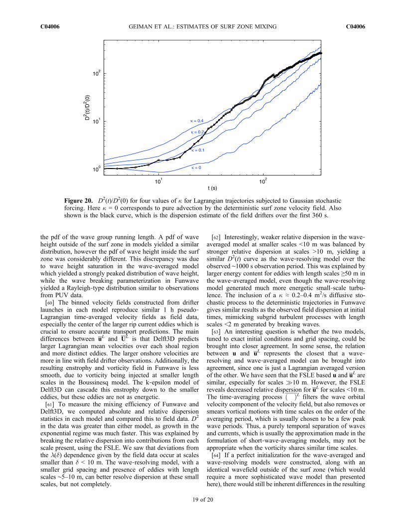
three patches of fluid particles inside the surf zone with andwithout the stochastic forcing in Figure 19 with = 0.2 m2/s.In the unperturbed case, particles tend to be stretched in longfilaments that extend offshore. The effect of the advective‐diffusive process is to increase the diffusion at initial times,with the long filamentary structures being homogenized intothe ambient fluid after less than 120 s.[57] In Figure 20, we again compute D2(t)/D2(0) as in

Figure 16 with D(0) = 2 m, but with several values of = (0,0.1, 0.2, 0.4) m2/s, along with the field D2 estimate. = 0 isthe case with pure advection by the velocity field u. There isfairly good agreement between the field data and smallvalues of ≈ 0.2–0.5 m2/s. The analysis presented by Brownet al. [2009] strongly suggests that the initial diffusion isassociated with small‐scale wave‐breaking induced turbu-lence and not with positional error. The corresponding valuefor this turbulent diffusivity on yearday 124 is 0.3 m/s2,which coincides with our estimated . At these scales, 3D

effects of both the drifter motion and water column itself areimportant as well.

8. Conclusions

[58] Output from the wave‐resolving model Funwave andthe wave‐averaged model Delft3D have been compared tobetter understand mixing contributions from surface gravitywave time scales in commonly used surf zone circulationmodels. Each model is able to reproduce 1 h time‐averagedmean Eulerian velocities consistent with field measurementsat stationary current meters. The spatial distribution of Hrms

inside the surf zone was different between the models, dueto the different mechanisms for wave breaking. This yieldeda more uniform Hrms(y) in the wave‐resolving model, whilewave height in the wave‐averaged model was much moreclosely tied to the alongshore bathymetry.[59] We showed that the wave forcing generated by each

model has a similar temporal group structure by looking at

Figure 19. (top) The advection by u (from Funwave) of three fluid blobs composed of 7000 particleseach, with = 0 at three successive times. (bottom) The effect of = 0.2 m2/s.


18 of 20

the pdf of the wave group running length. A pdf of waveheight outside of the surf zone in models yielded a similardistribution, however the pdf of wave height inside the surfzone was considerably different. This discrepancy was dueto wave height saturation in the wave‐averaged modelwhich yielded a strongly peaked distribution of wave height,while the wave breaking parameterization in Funwaveyielded a Rayleigh‐type distribution similar to observationsfrom PUV data.[60] The binned velocity fields constructed from drifter

launches in each model reproduce similar 1 h pseudo‐Lagrangian time‐averaged velocity fields as field data,especially the center of the larger rip current eddies which iscrucial to ensure accurate transport predictions. The maindifferences between uL and UL is that Delft3D predictslarger Lagrangian mean velocities over each shoal regionand more distinct eddies. The larger onshore velocities aremore in line with field drifter observations. Additionally, theresulting enstrophy and vorticity field in Funwave is lesssmooth, due to vorticity being injected at smaller lengthscales in the Boussinesq model. The k‐epsilon model ofDelft3D can cascade this enstrophy down to the smallereddies, but these eddies are not as energetic.[61] To measure the mixing efficiency of Funwave and

Delft3D, we computed absolute and relative dispersionstatistics in each model and compared this to field data. D2

in the data was greater than either model, as growth in theexponential regime was much faster. This was explained bybreaking the relative dispersion into contributions from eachscale present, using the FSLE. We saw that deviations fromthe l(d) dependence given by the field data occur at scalessmaller than d < 10 m. The wave‐resolving model, with asmaller grid spacing and presence of eddies with lengthscales ∼5–10 m, can better resolve dispersion at these smallscales, but not completely.

[62] Interestingly, weaker relative dispersion in the wave‐averaged model at smaller scales <10 m was balanced bystronger relative dispersion at scales >10 m, yielding asimilar D2(t) curve as the wave‐resolving model over theobserved ∼1000 s observation period. This was explained bylarger energy content for eddies with length scales ≥50 m inthe wave‐averaged model, even though the wave‐resolvingmodel generated much more energetic small‐scale turbu-lence. The inclusion of a ≈ 0.2–0.4 m2/s diffusive sto-chastic process to the deterministic trajectories in Funwavegives similar results as the observed field dispersion at initialtimes, mimicking subgrid turbulent processes with lengthscales <2 m generated by breaking waves.[63] An interesting question is whether the two models,

tuned to exact initial conditions and grid spacing, could bebrought into closer agreement. In some sense, the relationbetween u and uL represents the closest that a wave‐resolving and wave‐averaged model can be brought intoagreement, since one is just a Lagrangian averaged versionof the other. We have seen that the FSLE based u and uL aresimilar, especially for scales �10 m. However, the FSLEreveals decreased relative dispersion for uL for scales <10 m.The time‐averaging process ð ÞL filters the wave orbitalvelocity component of the velocity field, but also removes orsmears vortical motions with time scales on the order of theaveraging period, which is usually chosen to be a few peakwave periods. Thus, a purely temporal separation of wavesand currents, which is usually the approximation made in theformulation of short‐wave‐averaging models, may not beappropriate when the vorticity shares similar time scales.[64] If a perfect initialization for the wave‐averaged and

wave‐resolving models were constructed, along with anidentical wavefield outside of the surf zone (which wouldrequire a more sophisticated wave model than presentedhere), there would still be inherent differences in the resulting

Figure 20. D2(t)/D2(0) for four values of for Lagrangian trajectories subjected to Gaussian stochasticforcing. Here = 0 corresponds to pure advection by the deterministic surf zone velocity field. Alsoshown is the black curve, which is the dispersion estimate of the field drifters over the first 360 s.


19 of 20

current and vorticity fields. The major obstacle between acloser relation between u or uL and UL is the wave breakingparameterization, which is the source of disagreement inwave height distribution inside of the surf zone. Wavebreaking by short‐crested waves in the Boussinesq modelalso injects vorticity at length scales much smaller than thecurl of the radiation stress forcing, and it not clear thatrefining the grid spacing in the wave‐averaged model willaccount for the smaller length scale forcing.

[65] Acknowledgments. J.G. and J.K. are supported by the NationalScience Foundation Physical Oceanography Program through grant OCE0727376. A.R. was supported by ONR contract N00014‐07‐1‐0556 andthe National Science Foundation OCE 0927235. J.M. was supported byONR contract N00014‐05‐1‐0154, N00014‐05‐1‐0352, N00014‐07‐WR‐20226, N00014‐08‐WR‐20006, and the National Science FoundationOCE 0728324. Although many assisted in the data collection at RCEX,special thanks are due to Jeff Brown, Jenna Brown, and Tim Stanton fortheir vital role in collecting and processing the bathymetry, drifter, andADCP data used in this paper.

ReferencesAndrews, D. G., and M. E. McIntyre (1978), An exact theory of nonlinearwaves on a Lagrangian‐mean flow, J. Fluid Mech., 89, 609–646.

Artale, V., G. Boffetta, A. Celani, M. Cencini, and A. Vulpiani (1997), Dis-persion of passive tracers in closed basins: Beyond the diffusion coeffi-cient, Phys. Fluids, 9, 3162–3171.

Booij, N., R. C. Ris, and L. H. Holthuijsen (1999), A third‐generation wavemodel for coastal regions: 1. Model description and validation, J. Geo-phys. Res., 104, 7649–7666.

Brocchini, M., A. B. Kennedy, L. Soldini, and A. Mancinelli (2004), Topo-graphically controlled, breaking‐wave‐induced macrovortices. Part 1.Widely separated breakwaters, J. Fluid Mech., 507, 289–307.

Brown, J., J. MacMahan, A. J. H. M. Reniers, and E. Thornton (2009), Surfzone diffusivity on a rip‐channeled beach, J. Geophys. Res., 114,C11015, doi:10.1029/2008JC005158.

Bühler, O., and T. E. Jacobson (2001), Wave‐driven currents and vortexdynamics on barred beaches, J. Fluid Mech., 449, 313–339.

Chen, Q. (2006), Fully nonlinear Boussinesq‐type equations for waves andcurrents over porous beds, J. Eng. Mech., 220, 132–143.

Chen, Q., R. A. Dalrymple, J. T. Kirby, A. B. Kennedy, and M. C. Haller(1999), Boussinesq modelling of a rip current system, J. Geophys. Res.,104, 617–637.

Chen, Q., J. T. Kirby, R. A. Dalrymple, A. B. Kennedy, and A. Chawla(2000), Boussinesq modelling of wave transformation, breaking, and run-up. II: 2D, J. Waterw. Port Coastal Ocean Eng., 126, 48–56.

Chen, Q., J. T. Kirby, R. A. Dalrymple, F. Shi, and E. B. Thornton (2003),Boussinesq modelling of longshore currents, J. Geophys. Res., 108(C11),3362, doi:10.1029/2002JC001308.

Craik, A. D. D., and S. Leibovich (1976), A rational model for Langmuircirculations, J. Fluid Mech., 73, 401–426.

Goda, Y. (2000), Random Seas and Design of Maritime Structures, 2nded., World Sci., Singapore.

Holm, D. D. (1996), The ideal Craik‐Leibovich equations, Physica D, 98,415–441.

Johnson, D., and C. Pattiaratchi (2006), Boussinesq modelling of transientrip currents, Coastal Eng., 53(5), 419–439.

Kennedy, A. B., Q. Chen, J. T. Kirby, and R. A. Dalrymple (2000),Boussinesq modelling of wave transformation, breaking, and runup. I:1D, J. Waterw. Port Coastal Ocean Eng., 126, 39–47.

LaCasce, J. H. (2008), Statistics from Lagrangian observations, Prog.Oceanogr., 77(1), 1–29, doi:10.1016/j.pocean.2008.02.00.

Long, J. W., and H. T. Özkan‐Haller (2009), Low‐frequency characteristicsof wave group‐forced vortices, J. Geophys. Res., 114, C08004,doi:10.1029/2008JC004894.

Longuet‐Higgins, M. S., and R. Stewart (1962), Radiation stress and masstransport in gravity waves, with application to ‘surf‐beats,’ J. FluidMech., 13, 481–504.

MacMahan, J., et al. (2010), Mean Lagrangian flow behavior on open coastrip‐channeled beaches: New perspectives, Mar. Geol., 268, 1–15,doi:10.1016/j.margeo.2009.09.011.

MacMahan, J. H., A. J. H. M. Reniers, E. B. Thornton, and T. P. Stanton(2004), Surf zone eddies coupled with rip current morphology, J. Geo-phys. Res., 109, C07004, doi:10.1029/2003JC002083.

MacMahan, J., J. Brown, and E. B. Thornton (2009), Low‐cost handheldGlobal Positioning Systems for measuring surf zone currents, J. CoastalRes., 25(3), 744–754, doi:10.2112/08-1000.1.

Newberger, P. A., and J. S. Allen (2007), Forcing a three‐dimensional,hydrostatic primitive‐equation model for application in the surf zone:1. Formulation, J. Geophys. Res., 112 , C08018, doi:10.1029/2006JC003472.

Oltman‐Shay, J., P. A. Howd, andW.A. Birkemeier (1989), Shear instabilitiesof the mean longshore current: 2. Field observations, J. Geophys. Res.,94, 18,031–18,042.

Özkan‐Haller, H. T., and J. T. Kirby (1999) Nonlinear evolution of shearinstabilities of the longshore current: A comparison of observationsand computations, J. Geophys. Res., 104, 25,953–25,984.

Poje, A. C., and G. Haller (1999), Geometry of cross‐stream mixing in adouble‐gyre ocean model, J. Phys. Oceanogr., 29, 1649–1665.

Poje, A. C., A. C. Haza, T.M. Özgökmen,M. G.Magaldi, and Z. D. Garraffo(2010), Resolution dependent relative dispersion statistics in a hierarchy ofocean models, Ocean Modell., 31, 36–50.

Putrevu, U., and I. A. Svendsen (1999), Three‐dimensional dispersion ofmomentum in wave‐induced nearshore currents, Eur. J. Mech. B, 18,409–427.

Reniers, A. J. H. M., J. A. Roelvink, and E. B. Thornton (2004), Morpho-dynamic modeling of an embayed beach under wave group forcing,J. Geophys. Res., 109, C01030, doi:10.1029/2002JC001586.

Reniers, A. J. H. M., J. H. MacMahan, E. B. Thornton, T. P. Stanton,M. Henriquez, J. W. Brown, J. A. Brown, and E. Gallagher (2009), Surfzone retention on a rip‐channeled beach, J. Geophys. Res., 114, C10010,doi:10.1029/2008JC005153.

Roelvink, J. A. (1993), Dissipation in random wave groups incident on abeach, Coastal Eng., 19, 127–150.

Shepard, F. P., and D. L. Inman (1950), Nearshore water circulation relatedto bottom topography and refraction, Eos Trans. AGU, 31, 196–212.

Smith, J. A. (2008), Vorticity and divergence of surface velocities near-shore, J. Phys. Oceanogr., 38, 1450–1468.

Smith, J. A., and J. L. Largier (1995), Observations of nearshore circula-tion: Rip currents, J. Geophys. Res., 100, 10967–10976.

Spydell, M. S., and F. Feddersen (2009), Lagrangian drifter dispersion inthe surf zone: Directionally‐spread normally incident waves, J. Phys.Ocean., 39, 809–830.

Taylor, G. I. (1921), Diffusion by continuous movements, Proc. LondonMath. Soc., 20, 196–212.

Terrile, E., R. Briganti, M. Brocchini, and J. T. Kirby (2006), Topo-graphically induced enstrophy production/dissipation in coastal models,Phys. Fluids, 18, 126603, doi:10.1063/1.2400076.

Wei, G., J. T. Kirby, andA. Sinha (1999), Generation of waves in Boussinesqmodels using a source function method, Coastal Eng., 36, 271–299.

Yu, J., and D. N. Slinn (2003), Effects of wave‐current interaction on ripcurrents, J. Geophys. Res., 108(C3), 3088, doi:10.1029/2001JC001105.

J. D. Geiman and J. T. Kirby, Center for Applied Coastal Research,University of Delaware, Newark, DE 19716, USA. ([email protected])J. H. MacMahan, Department of Oceanography, Naval Postgraduate

School, Monterey, CA 93943, USA.A. J. H. M. Reniers, Applied Marine Physics, Rosenstiel School of

Marine and Atmospheric Science, University of Miami, Miami, FL33149, USA.


20 of 20

effects of wave averaging on estimates of fluid mixing … · effects of wave averaging on...

Documents