Evaluation of Buffer Width onHydrologic Function, Water Quality,

and Ecological Integrity of Wetlands

John Nieber, Principal Investigator Department of Bioproducts and Biosystems Engineering

University of Minnesota

February 2011Research Project

Final Report 2011-06

All agencies, departments, divisions and units that develop, use and/or purchase written materials for distribution to the public must ensure that each document contain a statement indicating that the information is available in alternative formats to individuals with disabilities upon request. Include the following statement on each document that is distributed: To request this document in an alternative format, call Bruce Lattu at 651-366-4718 or 1-800-657-3774 (Greater Minnesota); 711 or 1-800-627-3529 (Minnesota Relay). You may also send an e-mail to bruce.lattu@state.mn.us. (Please request at least one week in advance).

Technical Report Documentation Page 1. Report No. 2. 3. Recipients Accession No. MN/RC 2011-06

4. Title and Subtitle 5. Report Date

Evaluation of Buffer Width on Hydrologic Function, Water Quality, and Ecological Integrity of Wetlands

February 2011 6.

7. Author(s) 8. Performing Organization Report No. John L. Nieber, Caleb Arika, Christian Lenhart, Mikhail Titov, Kenneth Brooks

9. Performing Organization Name and Address 10. Project/Task/Work Unit No. Department of Bioproducts and Biosystems Engineering University of Minnesota 1390 Eckles Ave. St. Paul, MN 55108

CTS Project #2008042 11. Contract (C) or Grant (G) No.

(c)89261 (wo) 61

12. Sponsoring Organization Name and Address 13. Type of Report and Period Covered Minnesota Department of Transportation Research Services Section 395 John Ireland Blvd, MS 330 St. Paul, MN 55155

Final Report 14. Sponsoring Agency Code

15. Supplementary Notes http://www.lrrb.org/pdf/201106.pdf 16. Abstract (Limit: 250 words) Human activities including agricultural cultivation, forest harvesting, land development for residential housing, and development for manufacturing and industrial activities can impair the quality of water entering the wetland, thereby detrimentally affecting the natural ecological functions of the wetlands. This can lead to degradation of biota health and biodiversity within the wetland, reduced water quality in the wetland, and increased release of water quality degrading chemicals to receiving waters. Under natural conditions wetlands develop buffer areas that provide some protection from the natural processes occurring on adjacent areas of the landscape. Buffers serve the function of enhancing infiltration of surface runoff generated on adjacent areas, thereby promoting the retention of nutrients in the soil, and retention of sediment suspended in the runoff water, while still allowing runoff water to reach the wetland through subsurface flow routes. To protect wetlands and receiving waters downstream from the wetlands it is important that wetlands in areas disturbed by human activities be provided with sufficient buffer to prevent degradation of wetland biotic integrity as well as degradation of wetland water quality. The question arises, “How much buffer is sufficient?” The objective of this study was to investigate the sufficiency of buffers to protect wetland biotic integrity and water quality, and to evaluate the benefits extended to wildlife by the habit available in wetland buffers. The study was conducted by using a wetland data base available for 64 wetlands in the Twin Cities metro area.

17. Document Analysis/Descriptors

Wetlands, Wetland buffers, Water quality, Index of Biologic Integrity, Buffer width, Wildlife, Habitat, Life histories, Hydrologic modeling, Hydrologic cycle, Cluster analysis

18. Availability Statement No restrictions. Document available from: National Technical Information Services, Alexandria, Virginia 22312

19. Security Class (this report) 20. Security Class (this page) 21. No. of Pages 22. Price Unclassified Unclassified 182

Evaluation of Buffer Width on Hydrologic Function, Water Quality, and Ecological Integrity of Wetlands

Final Report

Prepared by:

John L. Nieber

Caleb Arika Chris Lenhart Mikhail Titov

Department of Bioproducts and Biosystems Engineering

University of Minnesota

Kenneth Brooks

Department of Forest Resources University of Minnesota

February 2011

Published by:

Minnesota Department of Transportation Research Services Section

395 John Ireland Boulevard, Mail Stop 330 St. Paul, Minnesota 55155

This report represents the results of research conducted by the authors and does not necessarily represent the views or policies of the Minnesota Department of Transportation or the University of Minnesota. This report does not contain a standard or specified technique.

The authors, the Minnesota Department of Transportation, and the University of Minnesota do not endorse products or manufacturers. Any trade or manufacturers’ names that may appear herein do so solely because they are considered essential to this report.

Acknowledgments

This research work represents a cooperative effort between the Department of Bioproducts and Biosystems Engineering of the University of Minnesota, and the Minnesota Department of Transportation (Mn/DOT). We are grateful to the Mn/DOT for providing funding for the project. The necessary linkages with Mn/DOT during the course of the project, guidance, technical advice, and support, were willingly and expertly provided by Kenneth Graeve (Mn/DOT), Sarma Straumanis (Mn/DOT and BWSR), and Shirlee Sherkow (Mn/DOT Research Services Section), and have been greatly appreciated. Members of the Technical Advisory Panel included Bill Bartodziej (Ramsey Washington Metro Watershed District), Scott Carlson (Mn/DOT), Jack Frost (Met Council), Mark Gernes (MPCA), Kenneth Graeve (Technical Liaison), Sarma Straumanis, Shiree Sherkow (Administrative Liaison), Dan Shaw (BWSR), and Paul Walvatne (Mn/DOT). The contributions from these individuals in terms of attending TAP meetings, reviewing task reports, and offering assistance are greatly appreciated. We would also like to acknowledge the contributions to project GIS analysis provided by Mr. Jeremy Lund and Mr. Jason Ulrich. Facilities, equipment and administrative support were provided by the Department of Bioproducts and Biosystems Engineering of the University of Minnesota, and are here gratefully acknowledged.

Table of Contents

Chapter 1 Introduction................................................................................................................. 1

Scope ............................................................................................................................................1

Methods........................................................................................................................................2

Summary ......................................................................................................................................2

Chapter 2 Developing the Wetland Buffer Database ................................................................ 4

Introduction ..................................................................................................................................4

Data of buffer strips and wetlands runoff contributing areas ......................................................4

Wetland data ................................................................................................................................5

Processing and analysis of collected data ..................................................................................11

Wetland buffer size/width ..........................................................................................................11

Hydroperiod analysis .................................................................................................................20

Statistical analysis ......................................................................................................................27

Chapter 3 Analysis of Wetland Hydroperiod ........................................................................... 28

Introduction ................................................................................................................................28

Wetlands hydroperiod ................................................................................................................29

Spectral analysis.........................................................................................................................30

Analysis of data..................................................................................................................... 30

Wetland classification ........................................................................................................... 33

Hydroperiod and wetland biological health .......................................................................... 34

Evaluation of periodograms for wetlands monitored by Anoka Conservation District ........ 35

Discussion ..................................................................................................................................39

Chapter 4 Statistical Analysis of Collated Wetland Data ....................................................... 42

Data for analysis ........................................................................................................................42

Archived MPCA data ............................................................................................................ 42

GIS analysis .......................................................................................................................... 43

Linear regression ................................................................................................................... 43

Multidimensional scaling ...................................................................................................... 47

Recursive partitioning ........................................................................................................... 48

Intermediate conclusion ........................................................................................................ 49

Clustering of wetlands by similar soils ................................................................................. 50

Analysis of hydroperiod for subject wetlands ...................................................................... 55

Data inconsistency ................................................................................................................ 56

Overall conclusions ....................................................................................................................59

Chapter 5 Wetland Buffer Assessment Tool ............................................................................ 61

Introduction ................................................................................................................................61

Wetland buffers for wildlife .......................................................................................................62

Buffer width and area............................................................................................................ 62

Vegetative diversity .............................................................................................................. 62

Vegetative structure .............................................................................................................. 63

Connectivity .......................................................................................................................... 63

Life history needs of animals ................................................................................................ 63

Herpetiles: reptiles and amphibians ...................................................................................... 64

Birds ...................................................................................................................................... 64

Mammals............................................................................................................................... 68

Insects ................................................................................................................................... 68

Wetland buffers for water quality ..............................................................................................69

Wetland buffer assessment tool .................................................................................................71

Benefits to wildlife ................................................................................................................ 71

Benefits to individuals or closely related groups (Appendix A) ........................................... 72

Connectivity to adjacent landscapes ..................................................................................... 72

Wetland buffer assessment tool, Metric 3 ............................................................................. 76

Potential future vegetation assessment tools ......................................................................... 77

Benefits for water quality...........................................................................................................77

Cumulative percent removal ................................................................................................. 77

Infiltration modification of water-quality score .................................................................... 79

Slope modification of water-quality score ............................................................................ 79

Channelized flow modification of water-quality score ......................................................... 80

Summary and conclusion ...................................................................................................... 80

Chapter 6 Predicting Wetland Buffer Benefits Using the Assessment Tool.......................... 83

Background ................................................................................................................................83

Methods......................................................................................................................................83

Results ........................................................................................................................................83

Discussion ..................................................................................................................................86

Conclusions and recommendations for improvements ..............................................................89

Overall................................................................................................................................... 89

Wildlife ................................................................................................................................. 89

Water quality ......................................................................................................................... 89

Chapter 7 Discussion, Summary and Conclusion .................................................................... 90

References Cited.......................................................................................................................... 94

Appendix A. Life History Tables ............................................................................................... 99

Appendix B. Case Study: Planning Buffers for Blanding’s Turtle

Appendix C. Time Series Analysis

Appendix D. Results of Analysis of Wetland Water Level Data for Anoka Conservation District

Appendix E. Hydrologic Modeling of Watershed/Wetland Complexes to Assess Wetland Hydroperiod

Appendix F. Annotated Bibliography

List of Figures

Figure 2.1 Classified slopes (%) of wetland runoff contributing areas in a section of the TCMA. 6

Figure 2.2 Soil Hydrologic Groups in wetland runoff contributing areas in a section of the TCMA. ............................................................................................................................................ 7

Figure 2.3 Distribution of hydric soils in wetland runoff contributing areas in a section of the TCMA. ............................................................................................................................................ 8

Figure 2.4 Drainage classification of wetland runoff contributing areas in a section of the TCMA.......................................................................................................................................................... 9

Figure 2.5 Descriptions of the wetland properties in the archived data provided by MPCA (Gernes and Helgen, 2002). .......................................................................................................... 16

Figure 2.6 Section of the TCMA DOQ showing some of the wetland boundaries and adjacent buffer strips traced using ArcGIS® 9.0 digitizing tools. .............................................................. 19

Figure 2.7 Section of the TCMA DOQ showing some of the wetland boundaries and adjacent buffer strips traced using ArcGIS® 9.0 digitizing tools. .............................................................. 20

Figure 2.8 Water level and temperature at well number 2 of the Riley Creek being monitored by the Mn/DOT. ................................................................................................................................. 21

Figure 2.9 Location of wetlands investigated by the MPCA and those monitored by the Anoka Conservation District. ................................................................................................................... 23

Figure 2.10 Water level measurements and precipitation at the Bunker Wetland in Coon Creek, Blaine, MN (ACD wetland monitoring program). (Well depth was 40 inches, so a reading of less than –40 indicates water levels were at an unknown depth greater than or equal to 40 inches.) . 24

Figure 2.11 Water level measurements and precipitation at the Carlos 181st Street Wetland, Sunrise River, Anoka, MN (ACD wetland monitoring program). (Well depth was 40 inches, so a reading of less than –40 indicates water levels were at an unknown depth greater than or equal to 40 inches.) ..................................................................................................................................... 24

Figure 2.12 Water level measurements and precipitation at the Carlos Avery Wetland, Sunrise River, Columbus, Anoka, MN (ACD wetland monitoring program). .......................................... 25

Figure 2.13 Water level measurements and precipitation at the Bannochie Wetland in Coon Creek, Blaine, MN (ACD wetland monitoring program). ............................................................ 25

Figure 2.14 Water level measurements at the Camp Three Wetland, Sunrise River, Columbus, Anoka, MN (ACD wetland monitoring program). ....................................................................... 26

Figure 2.15 Water level measurements for the East Twin Co. Park Wetland, Upper Rum River, Burns, Anoka, MN (ACD wetland monitoring program). (Well depth was 40 inches, so a reading of less than –40 indicates water levels were at an unknown depth greater than or equal to 40 inches.) .......................................................................................................................................... 26

Figure 3.1 Water-level time series data for indicated wetlands in Anoka, MN. ........................... 31

Figure 3.2 Proportion of the total number of days wetland water levels were monitored in which the level exceeded the indicated value. ......................................................................................... 39

Figure 3.3 Spectra of the water-level record for wetlands monitored by ACD. ........................... 40

Figure 4.1 Pair-wise scatter plot for fraction of area under certain soil hydrological group, width and ratio measures for buffer, and IBI scores (site type coloring: black-agricultural, red-reference, green-urban, green-unknown). ..................................................................................... 45

Figure 4.2 Linear regression for IBI scores for plants and invertebrates versus buffer measures, buffer width and contributing area versus buffer area ratio. ......................................................... 46

Figure 4.3 Linear regression by site type (dots and solid - reference, triangles & dash - urban, x and dot-dash - agricultural site). ................................................................................................... 47

Figure 4.4 Multidimensional reduction for wetland water chemistry. .......................................... 48

Figure 4.5 Relaxed decision tree for plant IBI (1-area fraction with hydraulic conductivity, 2-buffer width (here in meters)). ...................................................................................................... 51

Figure 4.6 Scatter of invertebrate IBI and chloride levels per wetland (point) (data points are jittered and color is irrelevant. That is done to distinguish wetlands). ......................................... 52

Figure 4.7 Chloride levels on log-scale sorted by standard deviation (top 7 sites have single measurement). ............................................................................................................................... 52

Figure 4.8 Low chloride sites. Number labels correspond to wetland site identification. ............ 53

Figure 4.9 Bayesian Information Criteria for spherical cluster models of equal and variable volumes. ........................................................................................................................................ 54

Figure 4.10 Compact clustering of wetland sites by soil composition. ........................................ 55

Figure 4.11 Invertebrates IBI versus averaged buffer width per cluster (blue-low, green-moderate, and red-high Cl on log-scale). Number labels correspond to wetland site identification........................................................................................................................................................ 57

Figure 4.12 Invertebrates IBI vs. buffer to wetland area ratio per cluster (blue-low, green-moderate, red-high Cl on log-scale). Number labels correspond to wetland site identification. .. 58

Figure 4.13 Site 331 (04Rams064) sits within a single watershed, but the buffer stretches outside the watershed boundary. ............................................................................................................... 59

Figure 5.1 TSS removal efficiency based on buffer width. The equation used for the tool is the green line described by the equation: y = 8.50 Ln(x) + 51.53. .................................................... 70

Figure 5.2 Total phosphorous (TP) removal efficiency based on buffer width. The equation for the tool is the green line described by the equation: y = 15.84 Ln(x) + 5.9. ................................ 70

Figure 5.3 Total nitrogen (TN) removal efficiency based on buffer width. The equation used for the tool is the green line described by the equation: y = 20.24Ln(x) - 13.18. ............................. 71

Figure 5.4 40% connected wetland within 100 meters in Hugo, MN, a small town near the suburban fringe of the Twin Cities metro area. ............................................................................ 75

Figure 5.5 90 % connected wetland within 100 meters in Roseville, MN, a first-tier suburb of the Twin Cities metro area. ................................................................................................................. 75

Figure 5.6 Wetland Metric 2. Buffer score for benefit to wildlife based on width. The equation is weighted to the first 200 feet but recognizes that distances up to 900 feet are needed by many

animals to complete their life cycles. Buffer width is considered to be the maximum width of the buffer covering a minimum of at least 100m. ............................................................................... 76

Figure 5.7 Scaling of cumulative percentage of nutrient and sediment removal in vegetated buffers (% nitrogen, phosphorous and TSS removal) to a score ranging from 0-100. The cumulative removal % never reaches 100% for each category and therefore the maximum score is 250 rather than 300. Similarly the minimum removal % does not reach 0; even with a 5 foot buffer, cumulative removal % is approximately 115. ................................................................... 78

Figure 6.1 Cumulative scores for water quality and wildlife for ten wetlands in the Twin Cities region. According to the buffer assessment tool, water-quality benefits ranked consistently higher than wildlife benefits at all 10 wetlands. ........................................................................... 84

Figure 6.2 Scores for two components of the wildlife assessment too, the connectivity * human disturbance score and the width score, (vegetation scores are not shown). Based on width alone, the wetland buffers ranged from low to high for wildlife benefits, but the connectivity * human disturbance factor was low. ........................................................................................................... 85

Figure 6.3 Water-quality scores showing ranking (from 0-300) for sediment and nutrient removal efficiency of ten buffers in the Twin Cities metro region. According to the buffer assessment tool, based on width alone the buffers are highly effective at removing sediment and nutrients. However when modified for slope and hydrologic soil group, the buffers are predicted to be only moderately effective and expected to remove roughly half (1/3 to 2/3) of incoming sediment and nutrients......................................................................................................................................... 86

Figure 6.4 Distribution of infiltration rates in Twin Cities-area soils. The orange and yellow colors are associated with HSG A-B soils, the greens with HSG B – C, while the darker grays and blues are associated with HSG D. .......................................................................................... 88

List of Tables

Table 2.1 Proportion of wetland runoff contributing area evaluated from SSURGO soil data for select soil hydrologic groups. ....................................................................................................... 10 

Table 2.2 Proportion of wetland runoff contributing area in given drainage class evaluated from SSURGO soil data. ....................................................................................................................... 12 

Table 2.3 Sources of collected data sets. ...................................................................................... 13 

Table 2.4 Portion of wetlands monitoring data maintained by Minnesota Pollution Control Agency (Source: Mark Gernes, MPCA). ...................................................................................... 14 

Table 2.5 Wetlands and properties of area contributing runoff (extracted from master data table…). ........................................................................................................................................ 15 

Table 2.6 Measured buffer length around wetlands measurements conducted on-screen from DOQ data for wetlands in Ramsey County, MN. ......................................................................... 17 

Table 2.7 Measured buffer length around wetlands measurements conducted onscreen from DOQ data for wetlands in Hennepin County, MN. ................................................................................ 18 

Table 2.8 Wetland water level monitoring program, Anoka, MN (Anoka Natural Resources Web site developed and maintained by the Anoka Conservation District, Ham Lake, MN). ............... 22 

Table 3.1 Summary of wetlands’ water level and proportion of the entire monitoring period when water table is less than 1 foot below the ground surface. ............................................................. 32 

Table 3.2 Areas for wetland and surrounding buffer areas. .......................................................... 33 

Table 3.3 Wetlands and classification of plant species present. ................................................... 36 

Table 3.4 Hydroperiod analysis: percent of time period wetland water level is at or below indicated depth (below ground level). .......................................................................................... 41 

Table 5.1 List of herpetile species most likely to benefit from grass buffers on depressional wetlands of Twin Cities metro region, Minnesota*. ..................................................................... 65 

Table 5.2 Functional groups of wetland birds as described by Galatowitsch and van der Valk (1994). ........................................................................................................................................... 66 

Table 5.3 EOR bird species list (2001) for non-forested wetlands, confirmed, likely and possible species that occur in the western Twin Cities metro area, Minnesota. ......................................... 67 

Table 5.4 Individual species or functional group assessment: Life history categories used in the buffer assessment tool. .................................................................................................................. 72 

Table 5.5 Condition of adjacent landscape (from the wetland IBI for depressional wetlands developed by the Minnesota Pollution Control Agency (Gernes and Helgen, 2002). .................. 73 

Table 5.6 Wetland buffer assessment tool, Metric 1: Connectivity and habitat value of adjacent landscape (100m from wetland fringe). Examples of scoring are listed below. .......................... 74 

Table 5.7 Wetland buffer assessment tool, Metric 2: Wetland buffer width and value to wildlife. Benefits are ranked using the equation from Figure 5.6 (y= 2E-07x3 - 0.0004x2 + 0.3105x). .... 76 

Table 5.8 Wetland buffer assessment tool, Metric 3. ................................................................... 77 

Table 5.9 Tool for assessing benefit of wetland buffers for water quality. .................................. 78

Table 5.10 Influence of infiltration rate on buffer effectiveness. Buffer score modifier is multiplied times the score obtained from Table 5.9 and Figure 5.7. ............................................ 79

Table 5.11 Influence of slope on buffer effectiveness. Buffer score modifier is multiplied times the score obtained from Table 5.9 and Figure 5.7. Buffer effectiveness at water treatment declines with increasing slopes. To compensate for increased slopes, buffer lengths need to be increased as described in MN DNR (1995). ................................................................................. 80

Table 5.12 Summary of Mn/DOT wetland buffer assessment tool. ............................................. 81

Executive Summary

Runoff generated on areas contributing to wetlands help to sustain the hydrology, nutrient balances and plant life/wildlife of the wetlands. When the runoff generated is affected by human activity it can have a detrimental effect on the natural hydrologic balance of a wetland, and also adversely affect the quality of the wetland water as well as adversely affect the wetland plant and animal ecosystem. Buffers surrounding wetlands have the potential to protect the water quality and ecological quality of the wetlands from the stresses of human activities. Buffers serve to infiltrate excess water, excess nutrients and toxic substances, and also help to provide some shelter to wetland associated plants and animals from direct contact with adjacent human activities. This project attempted to address the question of how large should wetland buffers be to provide sufficient protection from human activities on adjacent lands. Currently the Wetlands Conservation Act (WCA) guideline is that a 50-foot buffer should be used as a minimum. Of course, there is development and economic pressures to minimize the buffer size because the greater the size of the buffer, the more land becomes unusable for development. Therefore, it is important to minimize the size of the buffer while not adversely affecting the hydrologic, water quality, and ecological health of the system. The attempt involved the acquisition of archived wetland data for a large data set involving a number of depressional wetlands located in the Twin Cities metro area (TCMA). These data were developed into a matrix and additional wetland and contributing area attributes were derived using GIS data and aerial photographic data. Derived parameters included the determination of watershed contributing area, and soil type descriptors, land slope, land use conditions for the contributing areas, and buffer width. Ecological health (Index of Biological Integrity) parameters and water-quality parameters were available from the archived data for each of the wetlands, which numbered 64. Statistical hypotheses, evaluated using the statistical package, R, were tested to determine whether a clear trend could be identified between the derived parameters and the Index of Biotic Integrity (IBI) scores and/or one or more of the water-quality parameters. Among all of the attempts none were successful to identify a relationship between the wetland conditions the water quality/ecological health for the wetland. It was concluded that to conduct a stronger analysis it will be necessary to acquire more detailed hydrologic, water quality, and ecological data for the wetland data set. In particular, it will be helpful to have recorded water levels and grab samples for water-quality parameters. This should be a goal for local units of government in each of the represented locales around the TCMA. A tool was developed for assessing wetlands for evaluating the buffer needs for water-quality protection and for wildlife habitat. Criteria for water-quality protection assessment were derived from the scientific literature summarizing results of experiments involving buffer size and capacity to buffer stormwater volume and water quality. Likewise, the criteria for wildlife habitat were derived from scientific studies reported in the scientific literature. The assessment tool was tested to evaluate the habitat for wildlife on a subset of the wetlands involved in this study.

1

Chapter 1 Introduction

Wetlands are an ecosystem formed by the intermittent presence or persistence of water in a depressional, flat or low topographic area. They are distinguished by the low velocity flow of water through them, their water tolerant (hydric) soils, and vegetation that is specifically adapted to grow in water (hydrophytes.) They are also notable for the types of wildlife that depend on these unique habitat characteristics. While wetlands are known to play an important hydrologic role in the remediation of sediment runoff and chemicals, they also have a limit to which they can do so effectively. If a wetland is subjected to excessive sedimentation, nutrient input or modification of the hydroperiod, its quality may become compromised and its ability to maintain crucial ecological diversity could be impaired. The upland area immediately adjacent to a wetland, referred to here as a buffer or riparian zone, is critical to wetland health. The dimensions, vegetative characteristics and soil composition, slope of these buffers, and their surrounding land use all determine how well they might assist in mitigation of the various types of runoff or deposition to the wetland. This research project intends to measure the buffer strip width parameter against the hydrologic and ecological quality of its adjacent wetland ecosystem in order to more clearly define the point at which we begin to see diminishing returns in the area of hydrologic function and ecological diversity.

Scope

In order to make an accurate assessment of buffer strip width effect on wetland function, it is critical to determine the type of wetland to be mitigated, the type of buffer adjacent to it, and the surrounding land use. Because it was only recently that the value of wetlands was discovered and documented, prior to the second half of the last century wetlands were considered of little value and most were drained for purposes of agricultural production or for other development objectives. With the awareness of their importance, however, many efforts have been made to restore drained wetlands and to protect those wetlands that remain. Globally, there are many different types of wetlands. For this project we will focus on inland freshwater wetlands, and of these we will further narrow our scope to Lacustrine systems which are defined here as wetlands existing in a depressional area or dammed river channel, having less than 30% cover of trees, shrubs, emergent vegetation or lichens, and being greater than 8 hectares (20 acres) in size, or Palustrine systems which are nontidal systems smaller than 8 hectares (20 acres) that are dominated by trees, shrubs and emergent vegetation. Within these types, we can further classify wetlands by their source of water. Some wetlands are regionally groundwater fed and tend to be more nutrient rich, with a distinct vegetative composition. Perched and depressional wetlands will tend to be nutrient-poor unless they are loaded from nutrient-rich runoff which can alter the type of plant community expected for the “natural” state of the system. There are also surface-groundwater interactions for wetlands that should be taken into consideration. Some wetlands allow for subsurface groundwater flow-through and others will discharge water on the soil surface into an adjacent aquatic system. When comparing the effects of buffer strip width and its attendant runoff, it is critical to identify

2

the type of wetland it is impacting so that the expected function of the wetland is accurately identified. Wetlands can serve a number of different functions, and public interest is always a factor; therefore, how the wetland is expected to look and behave will have to be determined and normalized as a response to buffer strip width. Several factors also affect the function of vegetated buffers and need to be accounted for when determining the effect of their width in relation to wetland function. The slope of the strip, vegetative and soil composition and antecedent moisture content all will impact the amount of nutrients, sediment and stormflow entering the wetland system (EOR, 2001; Ma et al., 2008). Some filter strips are composed of a heterogeneous mix of vegetation while others are simply grass. Some consist of sandy, loamy soils which allow for more water infiltration, decreasing stormflow runoff impacts; others may have a higher clay content which has higher runoff, but also facilitates adsorption of nutrients to soil particles. There has been more research conducted on the functioning of riparian buffers to aquatic systems than upland buffers to wetlands (Brooks et al., 2003). In fact, as established earlier, many wetlands are themselves considered buffers. This project is concerned with the effect of upland buffers to wetlands, but we have compiled information on constructed vegetative filter strips as well as natural riparian buffers. Although, technically, riparian buffers are the ecotone between an aquatic and upland zone (much the same as a wetland), research on their function has been collected in this case because it may be correlated to the way in which well-vegetated upland buffer strips function and may provide a basis for comparison as well.

Methods

In order to measure any detrimental impact wetlands may be experiencing, it will be necessary to assess their water quality and ecological composition. Hydrologic assessments are fairly straightforward and there are a number of modeling techniques that have been developed to measure the effect buffers have on nutrient, sediment and stormflow runoff. Much of this research has been conducted on buffer strip effects on adjacent aquatic systems, however, and recent studies indicate a need for more research on the correlation between buffer strip width and wetland functions specifically. Ecological measurements and modeling are more complex due to natural variability in species composition and their mobility. Recent research (Galatowitsch and Whited, 1999; Semlitsch and Bodie, 2003) indicates that measuring more than one trophic level of species would be most accurate in giving a holistic assessment of biological integrity. Once biological integrity is established and other factors of buffer and wetland characteristics are normalized it is more likely that a viable correlation may be established between the width of the buffer and the ecological functioning of the adjacent wetland.

Summary

While there are suggestions and guidelines (Wenger, 1999) for buffer strip widths around various types of ecosystems, there is no definitive guide that takes into account the many combinations of upland buffer and wetland ecosystem interactions. Compiling archived data on wetlands, ranking them into similar categories based on the above mentioned criteria, and determining

3

surrounding buffer width and composition may provide a basis for new standards, and possibly laws, regarding the interplay of these two systems. A definitive guide that compiles these criteria would simplify many future projects that have a possibility of impacting wetlands. Since all of this information may not be available from existing databases, it is anticipated that additional data acquisition and/or data manipulation will be required to supplement any archived data collected on this project. The time and effort required to acquire/developed this additional data, specifically the ecological portion, may be extensive, but is critical to an accurate assessment of the interplay between upland buffers and wetland ecosystems.

4

Chapter 2 Developing the Wetland Buffer Database

Introduction

Buffer strips are important features for the protection of ecological health of the wetlands. When placed around wetlands, they function by enhancing infiltration of surface runoff originating in upstream areas, thereby causing a reduction in sediment loads entering wetlands, at the same time promoting the retention of nutrients in the soil while still allowing runoff water to reach the wetland through subsurface flow (Brooks et al., 2003). Functional efficiency of the buffer strips depend on both the properties of the buffer strips and those of the physical environment they are placed in. The properties of buffer strips known to influence their performance include size, resident vegetation, soil properties, landscape topography, among others (Brooks et al., 2003; EOR, 2001). A primary objective of this project was to attempt to evaluate the relationships among buffer strip properties, wetland functioning and quality. This study has placed emphasis on the key buffer strip functions of stormwater infiltration, sediment trapping, and enhancing wetland water quality and wildlife diversity. The acquisition of archived data, development of additional data, and the analysis of the data with respect to wetland quality and functions are the main activities of this project. To achieve these objectives, the investigators started with the contents of the depressional wetlands report by Gernes and Helgen (2002) to identify specific wetlands in the Twin Cities metro area (TCMA) for analysis of buffer strip benefits to wetland quality. The report by Gernes and Helgen contained numerous attributes/characteristics for over 300 wetlands located around the State of Minnesota. Among the attributes/characteristics were the separate scores for vegetative and macroinertebrate Index of Biological Integrity, a human disturbance index, and selected water-quality parameters. From this database, a total of 64 metro area wetlands were selected. This chapter of the report provides an overview of the activities and procedures involved in processing existing data and deriving additional data from GIS and aerial photo databases.

Data of buffer strips and wetlands runoff contributing areas

Wetland functions are influenced by many factors. The properties and characteristics of buffer strips and lands adjacent to the wetlands have significant impact on the quantity and quality overland flow entering the wetlands (Brooks et al., 2003; EOR, 2001). Starting with the archived data referenced by Gernes and Helgen (2002), additional data on wetland contributing area and buffer area characteristics include:

hydrologic soil group (HSG) hydraulic conductivity hydric properties drainage class depth to restrictive layer representative topographic slope buffer width

5

Data sets on the above properties which were assembled from various sources, including the USDA/NRCS’s Soil Data Mart (SSURGO), were analyzed and mapped using the Soil Data Viewer® 5.2, and ArcGIS® 9.0 software. Figure 2.1 to Figure 2.4 show some of the outputs generated in the data processing and data analyses. The soils properties data is also contained in tables obtained from the analyses, and example of which is shown in Table 2.1. This data has been incorporated in a master table which has been created and applied in a statistical analysis -analysis designed to address some of the project objectives. The influence of each of the properties, including the soil hydrologic groups, on wetlands is determined mainly by the dominant class of the property. For example, in the Anoka 146 wetland shown in Table 2.1, the HSG A has a land cover of 956 out of the total 1793 acres of the wetland’s runoff contributing area. This implies that at least 50% (956/1793) of the influence of hydrologic soil properties on runoff being generated at this site is due to the effects of the HSG A.

Wetland data

An important indicator of the performance of a buffer strip is in the functioning and quality of the wetland the buffer is intended to protect. In this study, we have assembled data on various properties known to be indicative of wetland quality and functioning. These include:

A. Wetland physical properties, including o Wetland area o Size of runoff contributing area o Human disturbance scores of areas above wetland o Habitat alteration score o Hydrologic alteration score

B. Wetland chemical properties data, including o Water pH o Carbonates content o Chemical pollution score

C. Biological data, including o Plant Index of Biotic Integrity (IBI) o Invertebrate IBI o Animal species population diversity o Plant species population diversity

D. Wetlands monitoring data o time series water level data o precipitation

6

Figure 2.1 Classified slopes (%) of wetland runoff contributing areas in a section of the TCMA.

7

Figure 2.2 Soil Hydrologic Groups in wetland runoff contributing areas in a section of the TCMA.

8

Figure 2.3 Distribution of hydric soils in wetland runoff contributing areas in a section of the TCMA.

9

Figure 2.4 Drainage classification of wetland runoff contributing areas in a section of the TCMA.

10

Table 2.1 Proportion of wetland runoff contributing area evaluated from SSURGO soil data for select soil hydrologic groups.

A A/D B B/D C C/D D Other Total (acres)Anoka 146 959.60 174.37 16.13 359.49 0.00 0.00 0.00 283.93 1793.53Anoka 369 120.32 0.00 0.00 58.05 0.00 0.00 0.00 32.96 211.33Anoka 370 149.35 33.34 0.00 19.31 0.00 0.00 0.00 0.00 202.00Anoka 371 17.73 109.89 187.08 39.07 0.00 0.00 0.00 0.00 353.78Anoka 372 10.54 0.00 0.00 2.35 0.00 0.00 0.00 0.00 12.89Dakota 381 11.82 0.00 242.79 86.04 0.00 0.00 0.00 175.78 516.43Dakota 78 (Sunset) 453.31 66.97 1156.25 32.31 0.00 0.00 10.35 836.55 2555.75Hennepin 125 5.91 0.00 0.00 0.00 0.00 0.00 0.98 0.00 6.89Hennepin 139 126.51 0.00 31.79 12.75 0.00 0.00 150.19 1261.40 1582.65Hennepin 212 (TNC) 0.00 19.38 157.59 18.45 5.73 0.00 0.00 54.42 255.57Hennepin 213 0.00 0.00 66.05 0.00 0.00 0.00 0.00 9.95 76.00Hennepin 216 0.00 166.98 1894.89 307.69 59.56 54.11 0.00 446.15 2929.37Hennepin 218 (MNDOT) 0.00 21.74 162.52 8.25 4.31 0.00 0.00 6.29 203.11Hennepin 219 0.00 3.53 56.88 0.00 0.00 0.00 0.00 3.59 64.00Hennepin 220 0.00 15.32 206.02 6.34 0.00 0.00 0.00 72.55 300.22Hennepin 221 184.40 17.62 501.09 19.90 0.00 0.00 0.00 53.88 776.90Hennepin 222 0.00 0.00 9.36 0.00 0.00 0.00 0.00 348.86 358.22Hennepin 223 0.00 7.51 122.61 0.00 0.00 0.00 0.00 32.78 162.89Hennepin 274 0.00 22.10 378.91 104.03 0.00 0.00 0.00 395.63 900.68Hennepin 275 0.00 135.32 405.42 151.86 37.28 0.00 0.00 210.58 940.46Hennepin 390 0.00 1838.07 4104.74 1273.13 1269.94 100.55 0.00 1028.18 9614.61Hennepin 391 2.34 0.00 71.74 1.45 7.93 0.00 0.00 1.88 85.33Hennepin 49 (Leman's) 0.00 13.49 83.63 20.09 0.00 0.00 0.00 58.56 175.78Hennepin 53 (Grass) 0.00 0.00 5.10 0.00 0.00 0.00 0.00 400.45 405.55Hennepin 54 (Kasma) 0.00 34.63 184.30 63.84 76.35 0.00 0.00 0.01 359.13Hennepin 58 (Legion) 2.27 0.00 8.14 0.00 0.00 0.00 93.84 496.86 601.10Hennepin 59 (Lost1) 0.00 0.67 69.69 0.00 0.00 0.00 0.00 23.42 93.78Hennepin 62 (Mud) 0.00 12.21 74.90 3.66 0.00 0.00 0.00 21.01 111.78Hennepin 67 262.68 0.00 2.19 0.00 0.00 0.00 29.21 26.83 320.90Hennepin 80 (Turtle) 0.00 61.60 327.25 15.12 19.36 0.00 0.00 18.45 441.78Hennepin 83 (Wood Lake) 53.99 0.00 72.07 78.94 0.00 0.00 85.12 2828.08 3118.19Ramsey 124 30.80 0.00 82.21 5.18 0.00 0.00 0.00 195.14 313.33Ramsey 133 0.00 39.15 42.90 7.61 0.00 0.00 0.00 247.89 337.55Ramsey 136 3.71 3.94 74.65 1.70 0.00 0.00 0.00 1007.31 1091.31Ramsey 138 27.30 28.06 34.54 0.00 0.00 0.00 0.00 1378.51 1468.42Ramsey 144 30.80 0.00 82.21 5.18 0.00 0.00 0.00 195.14 313.33Ramsey 145 49.60 14.53 38.12 14.08 0.00 0.00 0.00 620.54 736.87Ramsey 316 3.35 13.70 35.72 0.00 2.51 0.00 0.00 20.93 76.22Ramsey 317 7.71 4.29 59.20 0.71 19.36 0.00 0.00 352.95 444.21Ramsey 318 0.00 15.01 95.89 1.41 12.30 79.16 0.00 0.00 203.77Ramsey 319 0.00 0.10 27.49 0.76 0.00 0.00 0.00 2.53 30.89Ramsey 320 2.22 5.57 12.35 0.00 2.51 0.00 0.00 5.56 28.22Ramsey 321 0.00 12.45 88.29 2.58 5.92 0.00 0.00 5.86 115.11Ramsey 323 2.13 0.00 232.75 23.91 52.26 0.00 0.00 54.27 365.32Ramsey 324 0.00 21.70 33.89 0.00 0.00 0.00 0.00 358.18 413.77Ramsey 326 0.00 0.00 22.68 0.00 0.45 0.00 0.00 4.21 27.33Ramsey 327 0.00 0.00 109.71 12.96 28.86 0.00 0.00 46.90 198.44Ramsey 328 249.18 400.14 1861.22 207.02 263.99 13.35 0.00 2274.98 5269.88Ramsey 331 1.99 4.04 20.91 0.00 2.42 0.00 0.00 37.97 67.33Ramsey 333 21.92 307.08 856.38 47.17 177.53 0.00 0.00 410.76 1820.85Ramsey 418 62.72 402.65 1254.08 100.17 200.57 0.00 0.00 837.95 2858.15Ramsey 419 0.00 23.17 7.41 0.00 0.00 0.00 0.00 179.64 210.22Ramsey 44 (Casey) 0.00 0.00 40.77 0.00 0.00 0.00 0.00 343.67 384.44Ramsey 52 (Jones) 99.23 42.72 138.76 7.81 0.00 0.00 0.00 3264.31 3552.83Ramsey 68 (Rose Golf) 0.00 0.00 27.06 0.00 0.00 0.00 0.00 486.27 513.32Ramsey 69 (Round) 0.00 2.75 18.96 0.00 0.00 0.00 0.00 42.29 64.00Ramsey 70 (Savage) 0.00 12.03 22.23 0.00 0.00 0.00 0.00 196.19 230.44Ramsey 82 (Wakefield) 0.00 5.94 127.29 0.00 4.05 12.00 0.00 769.36 918.65Scott 422 0.00 108.95 1257.82 290.49 0.00 0.00 0.00 11.17 1668.43Scott 423 0.00 15.11 192.58 28.21 0.00 0.00 0.00 0.54 236.44Scott 424 0.00 1.16 11.09 1.09 0.00 0.00 0.00 0.00 13.33Washington 435 0.00 9.79 49.88 8.33 0.00 0.00 0.00 0.00 68.00Washington 436 31.73 22.81 167.38 1.44 0.00 0.00 0.00 9.96 233.33Washington 437 0.00 1.99 41.01 0.00 3.66 0.00 0.00 0.00 46.67

Area (acres) within Hydrologic GroupSite Name

11

Identifying the sources of this data was accomplished with the assistance of members of the project Technical Advisory Panel. Various federal, state and local agencies involved in the monitoring studies and recording of information related to wetland hydrology, geographical location, contributing watershed conditions, and biological integrity have been helpful with requests for assistance with gaining access to the data. The sources of the data which were assembled are identified in Table 2.3.

Processing and analysis of collected data

Data processing and analysis was conducted with the aim of facilitating statistical analysis of the data on buffer strips and wetlands quality and functioning. To facilitate the analysis, it was determined that the data on certain properties of buffer strips, wetlands, and lands contributing runoff into wetlands be assembled into a master data table. A portion of the wetlands data obtained and their sources are listed in Table 2.4Table 2.4. Further explanations of the variables measured are provided in Figure 2.5. A part of the master data base constructed is shown in Table 2.5.

Wetland buffer size/width

The wetlands data acquired from agency reports did not have information on width of buffer strips surrounding the wetlands. Because this data is critical in addressing of some of the project objectives, ArcGIS measurement tools were applied to standard United States Geological Survey’s Digital Orthophoto Quadrangles (DOQ), downloaded from the Minnesota Department of Natural Resources’ (DNR) Data Deli, to measure the observable width of buffer strips. Using ArcGIS digitizing tools, the extents of both the wetlands and adjacent buffer strips were traced. Figure 2.6 and Figure 2.7 show sections of wetlands and adjacent buffer strips which were digitized using ArcGIS ® 9.0 digitizing tools applied on the Digital Orthophoto Quadrangles (DOQs) of the TCMA. The area of each wetland and that of the adjacent buffer strip were both determined using the GIS tools. Buffer strips do not generally exist as a constant width area surrounding the wetland itself. Generally the buffer strips are quite non-uniform in width. To account for this aerial photography was used to determine the buffer width in eight cardinal directions, north, northeast, east, southeast, south, southwest, west, and northwest. A sample of these width measurements is summarized in Table 2.6 and Table 2.7. All these data about buffer characteristics and wetland area were input to the aforementioned master table.

12

Table 2.2 Proportion of wetland runoff contributing area in given drainage class evaluated from SSURGO soil data. SW_Name Drainage Class Sum of

Acres Proportion of Area

Battle Creek excessively drained moderately well drained poorly drained somewhat excessively drained somewhat poorly drained very poorly drained well drained other

0.56 12.82 24.49 7.40 24.74 21.70 197.29 141.4

0.001 0.030 0.057 0.017 0.057 0.050 0.46 0.33

Battle Creek Total 430.40 1.00 Battle Creek Lake excessively drained

moderately well drained poorly drained somewhat excessively drained somewhat poorly drained very poorly drained well drained other

9.84 22.87 14.74 6.74 41.81 66.07 99.67 157.70

0.023 0.055 0.035 0.016 0.100 0.158 0.238 0.376

Battle Creek Lake Total 419.43 1.00 Beaver Lake excessively drained

moderately well drained poorly drained somewhat excessively drained somewhat poorly drained very poorly drained well drained other

12.41 3.04 15.91 3.29 23.35 87.65 228.52 69.18

0.028 0.007 0.036 0.007 0.053 0.198 0.515 0.156

Beaver Lake Total 443.36 1.0

13

Table 2.3 Sources of collected data sets. Contact Information Data Type Sources Marks Gernes; MPCA - South Biological Monitoring Unit, Environmental Outcomes and Analysis Division, 520 Lafayette Rd., St. Paul, MN 55155. (651) 297-3363 Mark.Gernes@state.mn.us

Wetlands data (physical, chemical, Biological)

Minnesota Pollution Control Agency (MPCA)

Simba Blood, Natural Resources Technician Ramsey-Washington Metro Watershed District

Wetland physical, chemical, biological data

Ramsey-Washington Watershed District

http://soildatamart.nrcs.usda.gov/Download.aspx?Survey=MN037&UseState=MN

Land and Soil data USDA Soil Data

USDA/NRCS

Jamie Schuborn, Water Resources Specialist; (763)438-2030 x12

Wetland water level ANOKA Water Conservation District

Karen Shragg, Manager; Wood Lake Nature Center 6700 Portland Ave. ,Richfield, MN 55423-2599; 612 861-9366; Scott Ramsay, Naturalist , SRamsay@cityofrichfield.org

Wetland water level Wood Lake Nature Center

Kenneth Graeve Botanist/Plant Ecologist, Office of Environmental Services, Mn/DOT, Mail Stop 620, 395 Ireland Blvd, St. Paul MN, 55155; (651)366-3613

Wetland water level Riley Creek, Benson, St. Bonifacious, and Big Dog wetlands

14

Table 2.4 Portion of wetlands monitoring data maintained by Minnesota Pollution Control Agency (Source: Mark Gernes, MPCA).

SiteNum SiteNameInvert rater year SiteType ImLandscape BufferDist HabitatAlt HydrolAlt ChemPol HDS CenUTMy Total36 Battle JCH MCG 1999 Urb 9 6 9 14 17.5 57.5 4976811.43 137 Bloom JCH MCG 1999 Ref 3 0 0 0 0 3 5191605.23 141 Breen JCH MCG 1999 Ag 15 15 12 10.5 17.5 74 4901302.48 143 Bunker JCH MCG 1999 Ag 6 6 9 0 3.5 27.5 5075069.47 144 Casey JCH MCG 1999 Urb 12 9 9 17.5 14 63.5 4985472.74 145 Cateract JCH MCG 1999 (blank) 3 3 3 0 10.5 20.5 5157564.81 146 Cuba JCH MCG 1999 Ag 18 9 15 21 14 81 5203223.41 147 Davis JCH MCG 1999 Ag 15 6 12 21 21 79 5199609.41 1

- - - - - - - - - - - - -84 Zager JCH MCG 1999 Ref 3 0 3 0 7 13 5075063.12 185 CWB (blank) 0 (blank) 0 0 0 0 0 0 5137980.77 1

116 Donley Small JCH MCG 1999 Ref 6 3 6 3.5 7 27.5 5212057.02 1124 (blank) (blank) 0 (blank) 0 0 0 0 0 0 4982494 1125 (blank) JG 2006 Ref 0 0 3 3.5 3.5 10 5004280 1354 (blank) JG 2005 Ref 6 0 6 0 3.5 15.5 5077327.21 1355 (blank) JG 2005 (blank) 9 6 12 21 14 63 5102176.01 1356 (blank) JG 2005 Ref 6 0 3 0 0 9 4861287.14 1357 Dot's Slough JG 2005 (blank) 12 3 3 7 10.5 35.5 4862692.34 1358 (blank) JG 2005 (blank) 3 0 0 0 7 10 4822037.93 1359 (blank) JG 2005 (blank) 6 0 3 0 3.5 13.5 4953051.94 1360 (blank) JG 2005 (blank) 9 3 9 10.5 3.5 36 5273575.83 1361 (blank) JG 2005 (blank) 9 6 6 7 14 43 5320903.81 1362 (blank) JG 2005 Ref 6 0 6 0 0 12 4952966.08 1365 (blank) JG 2005 (blank) 9 6 9 7 14 45 5132273.85 1367 (blank) JG 2006 (blank) 9 6 12 14 10.5 51.5 5077545.251 1368 JG 2006 (blank) 12 12 9 14 10.5 59.5 5004995.45 1

15

Table 2.5 Wetlands and properties of area contributing runoff (extracted from master data table…).

Anoka 372 0.18 9.12 3.77 0.00 0.00 0.00 0.00 0.00 0.00 0.00 12.89 10.54 0.00 0.00 2.35 0.00 0.00 0.00 0.00Dakota 381 0.22 231.32 163.89 97.36 21.53 2.34 0.00 0.00 175.78 328.83 11.82 11.82 0.00 242.79 86.04 0.00 0.00 0.00 175.78Dakota 78 (Sunset) 0.02 225.38 1247.13 327.20 496.86 223.14 0.62 35.42 842.27 993.05 720.43 453.31 66.97 1156.25 32.31 0.00 0.00 10.35 836.55Hennepin 125 0.14 0.98 1.69 2.17 2.05 0.00 0.00 0.00 0.00 0.00 6.89 5.91 0.00 0.00 0.00 0.00 0.00 0.98 0.00Hennepin 139 0.15 502.30 951.72 8.91 0.00 0.00 119.72 0.00 1261.40 0.94 320.30 126.51 0.00 31.79 12.75 0.00 0.00 150.19 1261.40Hennepin 212 (TNC) 0.21 92.25 47.96 66.86 11.01 0.00 37.67 0.00 54.42 157.02 44.12 0.00 19.38 157.59 18.45 5.73 0.00 0.00 54.42Hennepin 213 0.12 11.89 31.70 20.65 3.28 0.00 8.48 0.00 9.95 66.05 0.00 0.00 0.00 66.05 0.00 0.00 0.00 0.00 9.95

All Hydric Not Hydric Partially Hydric Unknown Hydric

Excessively drained

Somewhat exc. drained

Well drained

Mod. well drained

Poorly drained

Somewhat poorly drained

Very poorly drained

Water Other 0- 200 inch >200 inch

534.29 1011.49 10.42 238.76 782.58 0.00 0.00 16.13 13.11 177.02 520.76 60.3 223.6 0.00 1793.5358.10 120.41 0.00 32.99 101.34 0.00 0.00 0.00 0.00 18.98 58.05 0.0 33.0 0.00 211.3352.69 149.47 0.00 0.00 119.51 0.00 0.00 1.72 0.00 28.12 52.65 0.0 0.0 0.00 202.00149.08 204.97 0.00 0.00 0.00 0.00 171.02 33.80 4.27 0.00 144.70 0.0 0.0 0.00 353.782.35 10.54 0.00 0.00 7.26 0.00 0.00 0.00 0.00 3.28 2.35 0.0 0.0 0.00 12.8986.11 319.23 0.00 111.50 11.82 17.35 211.12 9.11 74.50 5.21 11.54 111.4 64.4 0.00 516.43109.72 2145.82 0.00 302.22 453.31 200.15 867.10 64.21 12.31 19.08 97.32 41.3 801.0 3.10 2552.660.98 5.91 0.00 0.00 5.91 0.00 0.00 0.00 0.00 0.00 0.98 0.0 0.0 0.00 6.89150.31 128.93 42.26 1262.40 126.51 2.31 0.00 28.54 12.75 0.94 150.19 239.6 1021.8 0.00 1582.6522.85 19.45 158.99 54.46 0.00 19.44 117.13 11.38 15.00 15.37 22.84 54.4 0.0 0.00 255.570.00 8.90 57.20 9.96 0.00 0.00 54.98 6.42 0.00 4.65 0.00 9.2 0.8 0.00 76.00

Area (acres) within Hydric Group Area (acres) within Drainage Class Area (acres) within Depth ClassDepth to restrictive layer

Proportion of area in Class

0-1 2-5 6-9 10-15 16-20 21-30 >30 Low: (0.01 to 0.1 micrometers/s)

Moderately high (1 to

10)

High (10 to 100)

A A/D B B/D C C/D D Other

Anoka 146 0.04 864.28 875.03 54.22 0.00 0.00 0.00 0.00 283.93 0.00 1509.60 959.60 174.37 16.13 359.49 0.00 0.00 0.00 283.93Anoka 369 0.27 114.95 96.38 0.00 0.00 0.00 0.00 0.00 32.96 0.00 178.37 120.32 0.00 0.00 58.05 0.00 0.00 0.00 32.96Anoka 370 0.01 79.72 120.16 2.12 0.00 0.00 0.00 0.00 0.00 0.00 202.00 149.35 33.34 0.00 19.31 0.00 0.00 0.00 0.00Anoka 371 0.09 148.96 103.28 46.88 38.67 0.00 15.98 0.00 0.00 185.43 168.35 17.73 109.89 187.08 39.07 0.00 0.00 0.00 0.00

Name Area of Watershed under Slope Class (%) Area (acres) within KSat (x 0.001mm/s) Area (acres) within Hydrologic Group

16

Field Name Description Remarks//Detailed DescriptionsSiteNum Unique site serial numberSiteName Site nameCounty County site is located inArea_ha Site area in hectares Wetland AreaCenUTMx Centroid site coordinate in UTM X CoordinatesCenUTMy Centroid site coordinate in UTM Y coordinatesOwnership General ownership information

Buffer Disturbances 0=Best, no evidence of disturbance 6=Mod., predominately undisturbed, some human use influence 12=Fair, significant human influence, buffer area nearly filled with human use 18=Poor, nearly all or all of the buffer human use, intensive landuse surrounding wetlandLandscape (immediate influence) 0=Best, landscape natural, as expected for reference site, no evidence of disturbance 6=Moderate - predominately undisturbed, some human use influence 12=Fair, significant human influence, landscape area nearly filled with human use 18 = Poor, nearly all or all of the landscape in human use, isolating the wetlandHabitat alteration 0=Best, as expected for reference, no evidence of disturbance 6=Mod., low intensity alteration or past alteration that is not currently affecting wetland 12=Fair, highly altered, but some recovery if previously altered 18=Poor, almost no natural habitat present, highly altered habitatHydrologic alteration 0=Best, as expected for reference, no evidence of disturbance 7=Mod., low intensity alteration or past alteration that is not currently affecting wetland 14=Fair,less intense than “poor”, but current or active alteration 21=Poor, currently active and major disturbance to natural hydrologyChemical pollution 0=Best, chemical data as expected for reference and no evidence of chemical input 7=Mod., selected chemical data in low range, little or no evidence of chemical input 14=Fair, selected chemical date in mid range, high potential for chemical input 21=Poor, chemical input is recognized as high, with a high potential for biological harm

AddFact HDS factor, see Appendix 3 in Gernes and Helgen 2002

Additional factors - Used in exceptional cases

HDS Human Disturbance Score Human disturbance gradient score, derived from sources of data described above (rows 9-13), and scored as 5 factors, each factor judged and scored in one of 4 categories - best, medium, fair, & poor. Total points range from 0 for least disturbed to 100 most disturbed site.

LDI Landscape Development Intensity index based on 500 m buffer, see Bourdaghs et al. 2006

PropHumLandcover Proportional human dominated landcover in 500 m buffer, from 2001 NLCD

VisitDate Date sample was takenPlant IBI Plant based IBI score The plant metrics were based on (1) species richness of vascular and nonvascular taxa; (2)

community composition including Carex cover, aquatic species, perennial species and grasslike guilds; (3) tolerance and sensitivity measures; and (4) ecological process attributes based on dominance and persistent litter taxa.

Invert IBI Macro invertebrate based IBI score The invertebrate IBI is composed of ten metrics, each is scored and added into the total IBI score. The metrics include measures of taxa richness (in the 44 wetlands, 203 taxa observed with 187 genera), invertebrates that are intolerant of disturbance, and longer-lived invertebrates. Three metrics are based on proportions of certain more tolerant invertebrates that tend to increase under conditions of disturbance

Metadata of the MPCA Wetlands Data

BufferDist Within 50m buffer: HDS factor, see Appendix 3 (Gernes and Helgen, 2002)

ImLandscape Within 500m buffer: HDS factor, see Appendix 3 (Gernes and Helgen, 2002)

ChemPol HDS factor, see Appendix 3 in Gernes and Helgen 2002

HabitatAlt HDS factor, see Appendix 3 (Gernes and Helgen, 2002)

HydrolAlt HDS factor, see Appendix 3 in Gernes and Helgen 2002

Figure 2.5 Descriptions of the wetland properties in the archived data provided by MPCA (Gernes and Helgen, 2002).

17

Table 2.6 Measured buffer length around wetlands measurements conducted on-screen from DOQ data for wetlands in Ramsey County, MN.

+ The numeral before the star is distance along ray line from central ID point, and the number after asterisk is the distance perpendicular to nearest man-made disturbance.

18

Table 2.7 Measured buffer length around wetlands measurements conducted onscreen from DOQ data for wetlands in Hennepin County, MN.

+ The numeral before the star is distance along ray line from central ID point, and the number after asterisk is the distance perpendicular to nearest man-made disturbance.

19

Figure 2.6 Section of the TCMA DOQ showing some of the wetland boundaries and adjacent buffer strips traced using ArcGIS® 9.0 digitizing tools.

20

Figure 2.7 Section of the TCMA DOQ showing some of the wetland boundaries and adjacent buffer strips traced using ArcGIS® 9.0 digitizing tools.

Hydroperiod analysis

The persistence, or lack thereof, of water level/elevation in wetlands is known to impact biological diversity of wetlands. The data required to assess the effects of hydrologic alteration on wetland function/health would include water level data and water-quality sampling, in addition to biological monitoring. Unfortunately, water level records were available for only four of the wetlands within in the master data set, and then only for a short period of time. The wetlands included in the master data set that have had some recording of water level data include the Riley Creek, Benson, St. Bonifacious and Big Dog wetlands. Recording of these wetlands began in April 2008. A sample of wetland water level (and water temperature) data for the Riley Creek wetland is given in Figure 2.8.

21

-0.1

0

0.1

0.2

0.3

0.4

0.54/

14/2

008

4/20

/200

8

4/26

/200

8

5/3/

2008

5/9/

2008

5/15

/200

8

5/21

/200

8

5/28

/200

8

6/3/

2008

6/9/

2008

6/15

/200

8

6/22

/200

8

6/28

/200

8

7/4/

2008

Dates

Wet

alan

d W

ater

Lev

el (f

t)

0

5

10

15

20

25

Wat

er T

empe

ratu

re (F

)

LEVEL (ft.) TEMPERATURE

Figure 2.8 Water level and temperature at well number 2 of the Riley Creek being monitored by the Mn/DOT. Since hydroperiod was considered to be an important part of the assessment of wetland condition, and a possible indicator of wetland hydrologic alteration by human activity, it was of interest to find wetlands in a nearby area that have more extensive water level data. For this, 22 wetlands with water level data were identified in the Anoka Conservation District located north of the TCMA. Those wetlands are located on the map given in Figure 2.9 with summary information given in Table 2.8. The water level data for these wetlands were acquired from the Anoka Natural Resources website, developed and maintained by the Anoka Conservation District (ACD). The data is from water level recorded in wells located close to each of the 22 wetlands being monitored by the ACD. Measurements were made using the WL Ecotone, and WM series of devices from Remote Data Systems, Inc, installed in wells located in close proximity to the wetlands. Each of the units is capable of measuring water levels to a depth of 40 inches on a programmed schedule (4 hours) with accuracy of plus or minus 3 mm, and resolution of plus or minus 1 mm. The recording system accommodates for possible shifting of the well casing by frost heaving in winter. The district maintains records of water level, water temperature, and precipitation for all monitored wetlands. Figure 2.10 to Figure 2.15 show representative plots of data maintained for wells at a subset of these Anoka wetlands. A hydroperiod analysis was conducted on the water level data acquired for these 22 wetlands, and that hydroperiod analysis is reported in Chapter 3. It was desired to link hydroperiod to the ecological quality of wetlands, but after the hydroperiod analysis was completed it was discovered that IBI scores had not been collected for these wetlands. Therefore, the completed hydroperiod analysis serves as a good methods resource for future studies on hydroperiod analysis, but cannot be used for advancing the assessment of buffers on wetland quality.

22

Table 2.8 Wetland water level monitoring program, Anoka, MN (Anoka Natural Resources Web site developed and maintained by the Anoka Conservation District, Ham Lake, MN).

SiteID Water_Body_Name Project_Station_ID Watershed Municipality Lat UTM Long UTMAECWetland AEC Reference Wetland AEC Ref Wetland at old Anoka

Elec Coop/ConnexusLower Rum River Ramsey 5009281 465295.8

AlliantTechWetland Alliant Tech Reference Wetland

Alliant Tech Ref Wetland on Alliant Tech Property

Upper Rum River Burns 5026568.8 462094.8

BannochieWetland Bannochie Reference Wetland

Bannochie Ref Wetland near Radisson Rd and Hwy14

Coon Creek Blaine 5004733.5 483026.3

BunkerWetlandMiddle Bunker Reference Wetland

Middle of Bunker Ref Wetland at Bunker Hills Park

Coon Creek Andover 5007295.2 478493

CampThreeWetland Camp Three Reference Wetland

Camp Three Wetland in Carlos Avery WMA

Coon Creek Columbus 5011068 491566

Carlos181stWetland Carlos 181st Reference Wetland

Carlos181st Ref Wetland at 181st Ave in Carlos WMA

Sunrise River Columbus 5015997.7 495348.2

CarlosAveryWetland Carlos Avery Reference Wetland

Carlos Avery Ref Wetland at Carlos Avery WMA

Sunrise River Columbus 5018513.2 491129.5

CedarWetland Cedar Reference Wetland Cedar Ref Wetland at Cedar Creek Natural His Area

Upper Rum River East Bethel 5026967.6 484738.6

EastTwinWetland East Twin Reference Wetland

East Twin Ref Wetland in East Twin Co Park

Upper Rum River Burns 5019819.4 460432

GeorgeWetland George Reference Wetland

George Ref Wetland in Lake George Co Park

Upper Rum River Oak Grove 5023515.8 473154.8

IlexWetland Ilex Reference Wetland Ilex Ref Wetland in Oak Hollow Park on Ilex St

Coon Creek Andover 5011858.2 478274.4

IlexWetlandMiddle Ilex Reference Wetland Middle of Ilex Ref Wtld in Oak Hollow Park on Ilex

Coon Creek Andover 5011873.7 478266.2

KnollWetland Knoll Reference Wetland Knoll Ref Wetland at Knoll property

Coon Creek Ham Lake 5009296.8 487035.1

LampreyWetland Lamprey Reference Wetland

Lamprey Ref Wetland at Lamprey Pass WMA

Rice Creek Columbus 5011493.2 498243.8

PioneerParkWetland Pioneer Park Reference Wetland

Pioneer Ref Wetland at Pioneer Park

Coon Creek Blaine 5005520.3 483853.8

RCWDWetland RCWD Reference Wetland

RCWD Ref Wetland at Rice Creek Chain Park

Rice Creek Lino Lakes 5000973.5 493368.8

RumCentralWetland Rum Central Reference Wetland

Rum Central Ref Wetland in Rum Central Reg Park

Lower Rum River Ramsey 5015938 469814.7

SannerudWetlandEdge Sannerud Reference Wetland Edge

Edge of Sannerud Ref Wetland at Sannerud Prop

Coon Creek Ham Lake 5013017.4 481486.1

SannerudWetlandMiddle Sannerud Reference Wetland Middle

Middle of Sannerud Ref Wetland at Sannerud Prop

Coon Creek Ham Lake 5013045.8 481422

TamarackWetland Tamarack Reference Wetland

Tamarack Ref Wetland at Camp Salie

Sunrise River Linwood 5024515.9 493293.3

TargetWetland Target Reference Wetland

Target Ref Wetland at Target Co Dist Center

Rice Creek Fridley 4994094.1 480381.3

VikingWetland Viking Reference Wetland

Viking Ref Wetland at Viking Meadows Golf Course

Upper Rum River East Bethel 5018404 482301.8

23

Figure 2.9 Location of wetlands investigated by the MPCA and those monitored by the Anoka Conservation District.

24

Bunker Watershed Water Level Measurements (Coon Creek, Blaine)

-50

-40

-30

-20

-10

0

10

12/14/2005

3/24/2006

7/2/2006

10/10/2006

1/18/2007

4/28/2007

8/6/2007

11/14/2007

2/22/2008

6/1/2008

9/9/2008

12/18/2008

Date

Wat

er D

epth

(in)

0.0

0.5

1.0

1.5

2.0

2.5

Prec

ipita

tion

(in)

Water Level (in) Precip (in)

Figure 2.10 Water level measurements and precipitation at the Bunker Wetland in Coon Creek, Blaine, MN (ACD wetland monitoring program). (Well depth was 40 inches, so a reading of less than –40 indicates water levels were at an unknown depth greater than or equal to 40 inches.)

Carlos 181st Street Watershed Water Level (Sunrise River, Anoka)

-50

-40

-30

-20

-10

0

3/24/2

006

7/2/20

06

10/10

/2006

1/18/2

007

4/28/2

007

8/6/20

07

11/14

/2007

2/22/2

008

6/1/20

08

9/9/20

08

12/18

/2008

Date

Wat

er L

evel

(in)

0.0

0.5

1.0

1.5

2.0

2.5

3.0

Prec

ipita

tion

(in)

Water Level (in) Precip (in)

Figure 2.11 Water level measurements and precipitation at the Carlos 181st Street Wetland, Sunrise River, Anoka, MN (ACD wetland monitoring program). (Well depth was 40 inches, so a reading of less than –40 indicates water levels were at an unknown depth greater than or equal to 40 inches.)

25

Carlos Avery Watershed Water Level (Sunrise River, Anoka)

-50

-40

-30

-20

-10

0

10

10/28

/1995

3/11/1

997

7/24/1

998

12/6/

1999

4/19/2

001

9/1/20

02

1/14/2

004

5/28/2

005

10/10

/2006

2/22/2

008

7/6/20

09

Date

Wat

er L

evel

(in)

0.0

0.5

1.0

1.5

2.0

2.5

3.0

3.5

4.0

4.5

Prec

ipita

tion

(in)

Water Level (in) Precip ( in)

Figure 2.12 Water level measurements and precipitation at the Carlos Avery Wetland, Sunrise River, Columbus, Anoka, MN (ACD wetland monitoring program).

Bannochie Wetland Water Level (Coon Creek, Blaine)

-45

-40

-35

-30

-25

-20

-15

-10

-5

0

10/28

/1995

3/11/1

997

7/24/1

998

12/6/

1999

4/19/2

001

9/1/20

02

1/14/2

004

5/28/2

005

10/10

/2006

2/22/2

008

7/6/20

09

Date

Wat

er L

evel

(in)

0.0

0.5

1.0

1.5

2.0

2.5

3.0

3.5

4.0

4.5

Prec

ipita

tion

(in)

Water Level (in) Precip (in)

Figure 2.13 Water level measurements and precipitation at the Bannochie Wetland in Coon Creek, Blaine, MN (ACD wetland monitoring program).

26

Camp Three Watershed Water Level (Carlos Avery, Coon Creek, Anoka)

-30

-20

-10

0

4/22/2

008

5/12/2

008

6/1/20

08

6/21/2

008

7/11/2

008

7/31/2

008

8/20/2

008

9/9/20

08

9/29/2

008

Date

Wat

er L

Lev

el (i

n)

Precip Water Level (in)

Figure 2.14 Water level measurements at the Camp Three Wetland, Sunrise River, Columbus, Anoka, MN (ACD wetland monitoring program).

East Twin Co Park Watershed Water Level (Upper Rum River, Anoka)

-50

-40

-30

-20

-10

0

10

12/6/

1999

4/19/2

001

9/1/20

02

1/14/2

004

5/28/2

005

10/10

/2006

2/22/2

008

7/6/20

09

Date

Wat

er L

evel

(in)

0.0

1.0

2.0

3.0

4.0

5.0

6.0

7.0

Prec

ipita

tion

(in)

Water Level (in) Precip (in)

Figure 2.15 Water level measurements for the East Twin Co. Park Wetland, Upper Rum River, Burns, Anoka, MN (ACD wetland monitoring program). (Well depth was 40 inches, so a reading of less than –40 indicates water levels were at an unknown depth greater than or equal to 40 inches.)

27

Statistical analysis

The overarching hypothesis of this research is that wetland buffers tend to protect the hydrology and water quality of wetlands and that the larger the buffer the greater this protection. The data which would have been gathered and processed will be subjected to a series of analyzes to assess or identify any possible interrelations between wetland quality and functions, and the characteristics of adjacent buffer strips. Specific questions being asked are:

• How does the size (width) of the buffer strip affect water quality, biological diversity, and other functions of the protected wetland

• How do the properties, such as soil types and vegetation mixes of a buffer strip affect wetland quality and function

• Buffer strip connectivity and animal species populations and diversity

28

Chapter 3 Analysis of Wetland Hydroperiod

Introduction

Most wetlands in nature undergo water-level fluctuations in cyclic patterns which are influenced by seasonal change, tidal influence, and human activity (Mitsch and Gosselink, 1993). Water levels in most wetlands fluctuate seasonally, daily or semi-daily, or unpredictably. Pulsing hydroperiod (duration of inundation or substrate saturation) and flowing conditions enhance primary productivity and other ecosystem functions, which are frequently depressed by stagnant conditions (Mitsch and Gosselink, 2000). These fluctuations can have direct and indirect impacts on physical and biochemical processes in wetlands, hence affecting the local water quality and biological diversity. While wetland vegetation is known to be influenced by the interactions of many ecological factors, wetland hydrologic regime is most strongly correlated with the type of vegetation that establishes in the wetland complex (De Steven and Toner, 2004). Hydrological conditions, especially flooding regimes, are known to be a strong if not the primary influence on wetland plant community composition and processes (Mitsch and Gosselink, 1993; Keddy, 2000). Studies have shown that the processes of the nitrogen cycle can be significantly influenced by operator control of duration, sequence, and frequency of the wetland hydroperiod, influencing aerobic and anaerobic conditions in the system. While enhanced nutrient removal may be achieved through hydroperiod control, it is important to examine the effects of a created hydroperiod on other components of the system, particularly vegetation. A hydroperiod prescribed for nutrient control should also be conducive to adequate vegetative survival and productivity, especially in a system where significant nutrient removal can be attributed to assimilation by aquatic macrophytes. Water level fluctuation is a complex variable which encompasses not only the range, but also the frequency and regularity of change. According to Gopal (1999), the importance of a complete understanding of wetland functions and the response of resident plants and wildlife in natural wetlands utilized for wastewater treatment and constructed treatment wetlands can never be stressed enough. The different components of the water level regimes may affect the vegetation in different ways (Riis and Hawes, 2002). Studies have shown species diversity of aquatic vegetation to change in response to changes in the extent of level variation. For example, in some Canadian lakes species richness was low in lakes with little water level fluctuation (Hill and Keddy, 1992), higher in lakes with moderate water level fluctuations (Keddy and Reznicek, 1986; Wilcox and Meeker, 1991), but low again where fluctuations were extremely wide (Hill et al., 1998). In another study, Jansson et al. (2000) reported that species diversity of river bank vegetation was higher under unpredictable natural level variations than when variations were generated regularly by peaking flows from hydro-generating stations. Gosselink and Tumer (1978) have stated that hydroperiod, or hydraulic regime is the most important factor influencing wetland type or class, including inhabitant plant species and community makeup. The cyclic wet and dry periods affect the nitrogen cycle by creating cyclic aerobic and anaerobic conditions, thus controlling the occurrence and reaction rates of nitrification and denitrification.

29

The importance of hydroperiod (i.e. how long the wetland holds water) becomes immediately evident when we consider the larval period of some amphibian species. If the pond dries up before the larvae reaches metamorphosis, the larvae will die. For this reason, species with very long larval periods are excluded from breeding successfully in wetlands with short hydroperiods, because these don’t hold water long enough for the larvae to complete their development.

Wetlands hydroperiod

In the temperate regions, the most important source of water recharging wetlands is ice melt occurring during spring. Where significant amounts occur, rainfall is another primary source. Wetlands may be grouped into three categories based on the period of time they retain water; these are:

• Short hydroperiod wetlands: These are ephemeral wetlands that hold water for less than four months a year. In the northern temperate regions, these wetlands tend to dry by May, June or July of each year. Short hydroperiod wetlands are also considered “vernal pools.”

• Intermediate hydroperiod wetlands: These are ephemeral wetlands that hold water for at least four months (post ice-out) and tend to dry in late-July or later, or they dry only in years with low precipitation, so in some years they may hold water year-round. Intermediate wetlands often function as “vernal pools.

• Long hydroperiod wetlands: These are wetlands which hold water all year round without drying up. They are also known as “permanent” lakes or ponds.

These general hydroperiod categories are based, in part, on observed differences in the species of amphibians, aquatic invertebrates, and fish that tend to be present or absent from wetlands in each category. Hydroperiod of any given wetland can vary greatly from one year to the next, depending primarily on the amount of precipitation an area receives. In very dry years, a wetland may hold water for only a few weeks during the spring, but in very rainy years, that same wetland may hold water well into the summer. In other words, a wetland that normally functions as a short hydroperiod pond may function as an intermediate pond in years with abundant precipitation. The timing of precipitation is also critical for determining if a pond will provide amphibian breeding habitat in any given year. If a pond remains dry during the breeding and egg-laying period for any amphibian species, that pond will likely not provide breeding habitat for those amphibians that year, regardless if conditions change and the pool fills later in the season. These yearly differences in wetland hydroperiod can result in actual differences in the species of amphibians and aquatic insects that use or can successfully breed in any pond from one year to the next (Foster et al., 2007). Because water level variability in wetlands is important to biological and hydrological function, it would be valuable to quantify the time scale and magnitude of water-level fluctuations in order to fully understand hydroperiod. Important information to acquire includes:

• Identifying predominant hydroperiods of different wetlands

30

• Determine the range of water level fluctuations associated with predominant hydroperiods

• Investigate relationship between hydroperiod and given types of wetlands. There are several methods, such as the semi-variogram (Davis, 1986), harmonic analysis (Godin, 1972), higher order non-Fourier techniques (Kay and Marple, 1981), spectral analysis (Bendat and Piersol, 1986), and least-squares spectral methods (Vanícek, 1969; Lomb, 1976; Scargle, 1982) which can be used to examine frequency components of time series data, such as wetland water level fluctuations.

Spectral analysis

The analysis of time series data, such as wetland water levels over time was conducted using spectral analysis procedures. The details of those procedures are outlined in Appendix C. The methods were implemented in the programming language R® (R, 2009). The time series data analyzed for this study is described in Chapter 2 under the heading of hydroperiod analysis. The data were acquired from archived records held by the Anoka Conservation District, and apply to wetlands located outside of the TCMA. These data were used because time series data were not available for most of the TCMA, and even those few with time series data, the records were only two years long.

Analysis of data

The first part of the analysis was to construct simple plots of the time series data to allow for visual identification of trends and periodicity. A sample of the graphical results is presented in Figure 3.1. Plots for other wetlands are presented in Figure D.1 of Appendix D. These plots provide the key information on the range, the frequency and regularity of water level fluctuations. The plots also provided key information on the number of records and missing data, which are important in our decisions on appropriate methods for conducting further data analysis. Because water levels were monitored and recorded during warmer months of the year, there are obvious gaps in the data for all wetlands; however, some of the wetlands, such as Alliant, Carlos 181st, Bannochie, Bunker Coon Creek, and others show gaps during even warmer months of the year. These may be periods when monitoring could have been interrupted for various reasons, such as equipment malfunction. Selection of the appropriate data analysis method took into consideration the missing data. Table 3.1 is a presentation of the result of frequency analysis of the water level data for the different monitored wetlands in the Anoka data set. The proportion (p) of the total monitoring time that the water level stayed at the indicated water level depth (x-axis) or deeper (below ground surface) is as shown for a sample of the wetlands in Figure 3.2. Plots for other wetlands are presented in Figure D.2 in Appendix D. Research shows that when water level is above 12 inches of ground surface, the soil is considered for all practical purposes fully saturated. Wetlands which remain saturated (water level at 12 inches or less below ground surface) for longer durations would have a low p value corresponding to the 12-inch water level. This is important in determining if a given site is a wetland or not; and if so, what type of wetland.

31

Wetlands with mean water level greater than 12 inches (>-12 inches) and a low p value would be inundated longer periods of time. For example, Middle Sannerud with a mean water level of 1.93 inches below ground surface and a p value of 0.10 was inundated at least 90 percent of the entire time it was monitored. On the other end, wetlands with a large mean water level value, such as Knoll Coon Creek (32.57 inches) and a p value of 0.95 was inundated for only 5 percent of the total monitoring period.

Figure 3.1 Water-level time series data for indicated wetlands in Anoka, MN.

32

Table 3.1 Summary of wetlands’ water level and proportion of the entire monitoring period when water table is less than 1 foot below the ground surface.

33

Table 3.2 Areas for wetland and surrounding buffer areas.

Wetland classification

Based on obtained results of conducted analysis (summarized in Table 3.1), the wetlands used in this study could loosely be grouped into the three wetland classes based on mean water level and the p values as shown here below.

• Short hydroperiod wetlands (ephemeral wetlands that hold water for less than four months a year, i.e. less than 33% of the time, or p-value 0.67 or greater). Wetlands falling under this class include: AEC Ref, Alliant Tech, Bannochie, Bunker Coon Creek, Carlos 181St., ILEX ST., Knoll Coon Creek, Lake George, Lamprey Pass, Middle ILEX, Pioneer Park, RCWD Rice Creek, Rum Ramsy, Sannerud, Tamarack Sunrise, Target, and Viking

• Intermediate hydroperiod wetlands (ephemeral wetlands that hold water for at least four months (>33%, or p-value less than 0.67). Wetlands falling under this class include Carlos Avery, Cedar, East Twin, and Middle Sannerud.

34

• Long hydroperiod wetlands (wetlands which hold water all year round without drying up, also known as “permanent” lakes or ponds, i.e. nearly 100% of the time or p-value equal to 0). Wetlands falling under this class may include only Middle Sannerud with water level above 12 inches of ground surface 90% of the time.

Hydroperiod and wetland biological health

The water level data for the wetlands are presented in Figure D.1, while a sample of those data is illustrated in Figure 3.1. Visual analysis of the water level data show most of the wetlands having annual cycles of 2 peaks and troughs annually. Although the cycles may appear similar for different wetlands, the magnitudes and water levels differ significantly. This is obvious for Cedar and Ilex wetlands, with Ilex having much lower water levels. These plots on their own provide important information which can be applied in not only distinguishing between wetlands, but also predicting expected species community densities. Some of the key information includes the magnitude of fluctuations and the time period of inundation. Wetland hydroperiod is known to influence the ecological function and resultant plant community of a wetland. An objective of this study was to conduct an investigation on the relationship between wetland hydroperiod and plant species diversity for wetlands monitored by the Anoka Conservation District. As described earlier, time series water level data from monitoring over several years was acquired and subjected to analysis. There was however a lack of suitable vegetation data to be applied in the analysis. When data sets presented in Table 3.1and Table 3.3 were inspected and correlated, certain trends were observed. For example, Table 3.3 reveals that the wetlands, Carlos Avery, Cedar, and middle Sannerud, with high water table levels and large period of inundation (low p-value), have a larger percentage of their land area covered by obligate and/or wetland only facultative (FACW) plant species. On the other hand, those wetlands with especially low water table during most of the year (high p-value), such as AEC reference, Ilex street and Knoll Coon Creek, are noted as having a small portion of their total land area (about 10 percent ) populated by wetland (facultative) plant species. This result shows a positive utility to the hydroperiod analysis, but more biological monitoring is needed to fully utilize the spectral results. Inspection of the hydrographs show one or more predominant seasonal fluctuations, and smaller event-driven fluctuations. It can be observed that the timing of the minimum and maximum water-levels in different wetlands are consistent, but differ mainly in the relative water depths as well as in overall range of water-level fluctuations. Two distinct inter-annual periods of water-level fluctuations are observable. Although the magnitude of water-level varies, patterns remain constant from year to year. The variations from year to year in the hydroperiod are expected because these vary in respect of climate and antecedent conditions. The temporal cycles and the magnitude and duration of water-level fluctuations (hydroperiod) during the inter-annual cycles are important when describing wetland hydroperiod. Spectral analysis is useful in determining the overall temporal characteristics of periodicity, thus hydroperiod (Foster et al., 2007). Since ecological characteristics of a wetland are influenced by wetland hydroperiod, the periodicity of both inundation and water table fluctuations should be used in defining

35

hydroperiod and in investigating ecological function. Spectral analysis of the water-level time series for these wetlands was used in identifying dominant frequencies, which are representative of the hydroperiod and encompass the entire range of water-level fluctuations. Spectral estimates of water-level time series from 34 wetland observation wells indicate a distinct semi-annual peak periodicity, found to be significant with a 95% confidence interval. Table 3.3 provides information on class of plant species (wetland plant or not) found in different wetlands. This vegetation data was collected using the same methods as used for wetland delineations in Minnesota, as:

• Herbaceous vegetation - within 1 m of well • Shrubs - within 5 m of well • Trees - within 30 m of well

Evaluation of periodograms for wetlands monitored by Anoka Conservation District

A sample of the resulting periodograms evaluated from the available wetlands’ time series data is shown in Figure 3.3. Periodograms for other wetlands are presented in Figure D.3 in Appendix D. Spectral density data was plotted (log-log) against period. The smooth green line represents the theoretical spectrum for fitted autoregressive model with one parameter (AR(1) process). AR(1) spectrum is used as a null continuum to compare periodogram to. AR(1) fitting is not fully legitimate and is given for estimation only because of gap presence, i.e. non-fixed time step. The ten most distinct peaks of the periodogram from the AR(1) spectrum are shown (largest to smallest peak) in tables of period versus spectral power density (PSD) alongside the plots. The time series data are quite noisy data, therefore the resulting periodograms are noisy as well and extracted peaks are approximate with quite large error. The spectral peaks indicate the presence of dominant waveforms which represent the temporal component of hydroperiod and encompass the entire range of water-level fluctuations. There is a clear pattern of generally decreasing energy with decreasing time period. This quantifies the observation that storm event water-level fluctuations are much less intense than the dominant summer/fall and winter/spring water-level fluctuations. The plots show the semiannual and/or annual peaks being most common for these wetlands.

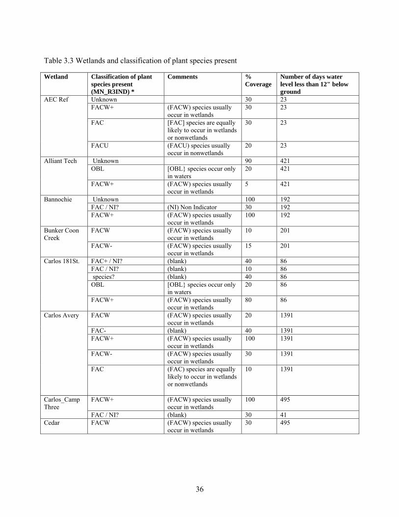
36

Table 3.3 Wetlands and classification of plant species present Wetland Classification of plant

species present (MN_R3IND) *

Comments % Coverage

Number of days water level less than 12" below ground

AEC Ref Unknown 30 23 FACW+ (FACW) species usually

occur in wetlands 30 23

FAC [FAC] species are equally likely to occur in wetlands or nonwetlands

30 23

FACU (FACU) species usually occur in nonwetlands

20 23

Alliant Tech

Unknown 90 421 OBL [OBL} species occur only

in waters 20 421

FACW+ (FACW) species usually occur in wetlands

5 421

Bannochie

Unknown 100 192 FAC / NI? (NI) Non Indicator 30 192 FACW+ (FACW) species usually

occur in wetlands 100 192

Bunker Coon Creek

FACW (FACW) species usually occur in wetlands

10 201

FACW- (FACW) species usually occur in wetlands

15 201

Carlos 181St.

FAC+ / NI? (blank) 40 86 FAC / NI? (blank) 10 86 species? (blank) 40 86 OBL [OBL} species occur only

in waters 20 86

FACW+ (FACW) species usually occur in wetlands

80 86

Carlos Avery

FACW (FACW) species usually occur in wetlands

20 1391

FAC- (blank) 40 1391 FACW+ (FACW) species usually

occur in wetlands 100 1391

FACW- (FACW) species usually occur in wetlands

30 1391

FAC (FAC) species are equally likely to occur in wetlands or nonwetlands

10 1391

Carlos_Camp Three

FACW+ (FACW) species usually occur in wetlands

100 495

FAC / NI? (blank) 30 41 Cedar FACW (FACW) species usually

occur in wetlands 30 495

37

Table 3.3 Wetlands and classification of plant species present (cont.). Wetland Classification of plant

species present (MN_R3IND) *

Comments % Coverage

Number of days water level less than 12" below ground

East Twin

FACW+ (FACW) species usually occur in wetlands

100 0

FACW (FACW) species usually occur in wetlands

20 0

FACW- (FACW) species usually occur in wetlands

10 0

ILEX ST.

Unknown 90 483 FACW+ (FACW) species usually

occur in wetlands 10 483

FAC / NI? (blank) 20 0 Knoll Coon Creek

FACW (FACW) species usually occur in wetlands

20 483

Lake George

NI? [NI] Not Indicator 20 760 FAC / NI? (blank) 40 483 FACU (FACU) species usually

occur in nonwetlands 30 483

Lamprey Pass

Unknown 90 550 OBL [OBL} species occur only

in waters 5 1100

FACW (FACW) species usually occur in wetlands

20 760

Middle Sannerud Middle/Center ILEX

OBL [OBL} species occur only in waters

40 41

OBL [OBL} species occur only in waters

20 139

FACW+ (FACW) species usually occur in wetlands

80 41

FACW+ (FACW) species usually occur in wetlands

100 139

FACW (FACW) species usually occur in wetlands

30 139

Pioneer Park

Unknown 40 259 FACW- (FACW) species usually

occur in wetlands 20 139

FACW (FACW) species usually occur in wetlands

20 259

FAC+ (FAC) species are equally likely to occur in wetlands or nonwetlands

10 139

FAC (FAC) species are equally likely to occur in wetlands or nonwetlands

20 259

RCWD Rice Creek

FACW+ (FACW) species usually occur in wetlands

40 850

FACW (FACW) species usually occur in wetlands

30 850

FACU+ (FACU) species usually occur in nonwetlands

30 259

38

Table 3.3 Wetlands and classification of plant species present (cont.). Wetland Classification of plant

species present (MN_R3IND) *

Comments % Coverage

Number of days water level less than 12" below ground

Rum Ramsy

Unknown (blank) 70 0 FACW+ (FACW) species usually

occur in wetlands 40 0

FAC+ / NI? (blank) 10 0 FACU (FACU) species usually

occur in nonwetlands 20 850

FACU- (FACU) species usually occur in nonwetlands

40 850

Sannerud

FACW+ (FACW) species usually occur in wetlands

40 918

FACW (FACW) species usually occur in wetlands

40 918

FAC (FAC) species are equally likely to occur in wetlands or nonwetlands

40 918

FAC (FAC) species are equally likely to occur in wetlands or nonwetlands

30 0

FACU+ (FACU) species usually occur in nonwetlands

10 0

Tamarack Sunrise

Unknown (blank) 70 70 OBL [OBL} species occur only

in waters 50 70

FACW+ (FACW) species usually occur in wetlands

10 70

FACU / NI? 70 918 Target

FACW (FACW) species usually occur in wetlands

100 539

FACW- (FACW) species usually occur in wetlands

20 539

FAC+ (FAC) species are equally likely to occur in wetlands or non-wetlands

10 70

FAC (FAC) species are equally likely to occur in wetlands or non-wetlands

75 539

Viking

FACW+ (FACW) species usually occur in wetlands

80 103

FACW+ (FACW) species usually occur in wetlands

100 138

FACW (FACW) species usually occur in wetlands

10 103

39

.81.

0x

Figure 3.2 Proportion of the total number of days wetland water levels were monitored in which the level was less than or equal to the indicated value. Table 3.4 is a summary extracted from plots in Figure 3.2. This table shows how much of the period within which water levels were being monitored for all the wetlands individual wetlands were inundated (water level above 12 inches from ground surface). Wetlands which are wet (inundated) during most of the monitoring period had a low percent value under the 30 inches depth and high values at 0 or 10 inch depths. For example, Middle Sannerud with water level at the 30 inch depth 0% of the time, and 20% at 10 inches or lower is rarely ever dry (water level at or deeper than 12 inches depth). On the other hand, wetlands such as Target Ref with 70% water level at 30 inches or deeper, and 95% at 10 inches or deeper, would be considered mostly dry (70% of the time). These trends in inundation are reflected in the types of vegetation species (obligates only in Middle Sannerud) covering the largest proportion of the area within the wetlands.

Discussion

The primary aim of conducting hydroperiod analysis in this project was to evaluate relationships between water level fluctuations and the functions and vegetation species diversity for the wetlands used in the study. However, available data for the wetlands (from Anoka County, Minnesota) was not sufficient for relevant analyses to establish these relationships. Spectral analysis of available time series water level data revealed mostly 2 annual peaks for most wetlands. The spectral analysis showed storm event water-level fluctuations for these wetlands (in Anoka) are much less intense than the dominant summer/fall and winter/spring water-level fluctuations. The plots show the semi-annual and/or annual peaks being most common for the wetlands.

-40 -35 -30 -25 -20 -15 -10

0.0

0.2

0.4

0.6

0

Water level, in

Prop

ortio

n <=

0.99

-12

AEC Ref

-30 -20 -10 0

0.0

0.2

0.4

0.6

0.8

1.0

Water level, in

Prop

ortio

n <=

x

0.594

-11.9

Alliant Tech

-30 -20 -10 0

0.0

0.2

0.4

0.6

0.8

1.0

Water level, in

Prop

ortio

n <=

x 0.882

-12

Bannochie

-30 -20 -10 0

0.0

0.2

0.4

0.6

0.8

1.0

Water level, in

Prop

ortio

n <=

x

0.611

-12

Bunker Coon Creek

40

A casual analysis of available vegetation data and the hydroperiod for different wetlands revealed expected trends. Wetlands which were inundated during most of the monitoring period were predominantly covered by species found mainly in wetlands, with limited or no upland species presence. More detailed biological monitoring data could reveal more telling information about the effect of hydroperiod on biological function/health.

Figure 3.3 Spectra of the water-level record for wetlands monitored by ACD.

41

Table 3.4 Hydroperiod analysis: percent of time period wetland water level is at or below indicated depth (below ground level).

Duration (% of monitoring period) water table is at or below indicated

depth (inches) Wetland ID 30 Inches 10 Inches 0 Inches AEC Ref 50 99 100 AlliantTech Ref 20 65 100 Bannochie Ref 40 85 100 BunkerMiddle Ref 20 78 100 CarloS181 Ref 50 85 100 CarlosAvery Ref 10 50 100 Cedar Ref 5 30 100 EastTwin Ref 15 60 100 Ilex Ref 62 95 - Knoll Ref 65 95 - L. George Ref 40 80 100 Lamprey Ref 20 70 100 Middle Ilex 40 88 100 Middle Sannerud 0 20 50 Pioneer Ref 40 80 100 Rum Central Ref 25 75 100 RWCD Ref 42 78 100 Sannerud Ref 30 95 - Tamarack Ref 20 50 85 Target Ref 70 95 - Viking Ref 40 70 100

42

Chapter 4 Statistical Analysis of Collated Wetland Data

A major objective of this project was to attempt to discover relationships between quantifiable biological indices and water-quality parameters in wetlands located in the TCMA and the size of the buffers surrounding those respective wetlands. The data for this analysis, described in Chapter 2, was derived from data archived by the MPCA and other agencies, and also from additional GIS analysis and hydroperiod analysis conducted within the scope of this project. A number of studies have been conducted to examine the impact of change in land use on the biological health and water-quality characteristics of wetlands, and it has been shown that significant changes in land use can have the effect of degrading wetlands in terms of both biological health as well as the water-quality measures (EOR, 2001). In the current project we examined the effect of buffering around a wetland to offset the effect of land use change. The hypothesis underlying this study is there is a relationship between buffer size (width) and the biological and water quality of the wetland receiving runoff water from the contributing watershed through the buffer. In the original project proposal it was stated that a meta-analysis would be conducted on the acquired wetland data. Meta-analysis is a collection of techniques to statistically combine the results of several independent studies that address shared research hypotheses to yield an overall answer to a question regarding the impact of an experimental treatment relative to a control treatment (e.g. Glass, 1976). The present study is based on a single data source for analysis and not independent studies regarding a particular treatment; therefore meta-analysis it is not suitable for the purposes of this project. However, the data set for the present project is certainly amenable to conventional statistical analysis, and attempts to apply several statistical methods using R project software (R Development Core Team, 2010).

Data for analysis

Chapter 2 of this report provides details of the data available for this project, including both the archived data as well as the data derived through the efforts of the current study for the same wetlands as those in the archived data. The procedures for deriving the archived data have been outlined in the report by Gernes and Helgen (2002), and those data were acquired for the current project through the assistance of Mark Gernes (MPCA, personal communication, 2008). The data derived within the scope of the current project were derived using GIS tools and aerial photography. A brief overview of the data acquired for the wetlands analyzed is presented below.

Archived MPCA data

MPCA prepared MS Access database with IBI scores and chemistry data (Gernes and Helgen, 2002) was used to assess wetland health. Wetland site type classification like

• Urban; • Agricultural; • Reference; • Unknown/unspecified

was used in an attempt to stratify the data.

43

Unfortunately IBI and chemistry data were found to be not available for every wetland on a regular basis within the archived data sets. There were also difficulties identifying and delineating the wetland buffer for some sites. Therefore number of involved wetland sites varies roughly from 45 to 61 depending on the type of analysis and data used.

GIS analysis

Wetlands, their buffer, and watershed area delineations were used to determine corresponding areas. Buffer delineation was done manually using aerial photography. Delineations were made for 61 sites. Area fractions from total wetland area of various soil parameters such as

• Slope; • Saturated hydraulic conductivity; • Hydrologic group; • Hydric class; • Drainage class

by classes of value ranges were also derived from GIS using NRCS SSURGO database. The following two buffer extent measures were proposed to conveniently quantify buffer size:

• Ratio of buffer area to wetland area • Averaged buffer width

Averaged buffer width is defined as the difference between the radii of the buffer and the wetland provided the assumption that buffer and wetland have round shape and are concentric. Note that for the purpose of convenience, most of the wetland sites are hereinafter referred by site number. In some cases names from the MPCA database corresponding to these numbers are given. The statistical methods applied in the buffer effectiveness analysis included linear regression, multidimensional scaling, recursive partitioning, and cluster analysis. The approach with each of these methods and the results derived in their applications are described in the following sections.

Linear regression

Linear relationships are unlikely to occur in complex systems containing many independent variables. It is therefore unlikely that a linear model of the system that attempts to relate a single dependent variable to a number of independent variables is likely to yield somewhat unsatisfactory results. Even so, a linear model is a good first step in an overall analysis to first establish the limitations of the linear model approach. As a result, the data set was subjected to a linear regression analysis. Scatter plots of pair-wise variables were examined. An example of such for few selected variables is shown in Figure 4.1. No apparent trend was found from this preliminary analysis;

44

however the relationship between IBI scores and buffer extent measure may be hidden by other factors. Linear regression for plant IBI score as a function of various variables did not shed light either. Though it seems that some variables (site area under certain slope class) have strong influence on plant IBI score, this relationship has many outliers and cannot be used for prediction. Plots of IBI versus both buffer extent measures are shown in Figure 4.2 and Figure 4.3 has data split by site type, i.e. urban, agricultural, reference, unknown. These plots do not manifest any noticeable trend and have scattered data points. As a result of the failure of the linear regression method, it was deemed necessary to stratify the data. That is, to look at the relationship between let’s say IBI score and other variables within the group of similar sites. The hypothesis is that similar sites should have less scatter between IBI score and buffer size.

45

Figure 4.1 Pair-wise scatter plot for fraction of area under certain soil hydrological group, width and ratio measures for buffer, and IBI scores (site type coloring: black-agricultural, red-reference, green-urban, green-unknown).

A

0.0 0.6 0.00 0.25 0.0 0.3 0 200 0 40 80

0.0

0.6

0.0

0.6

AD

B

0.0

0.6

0.00

0.25

BD

C

0.00

0.15

0.0

0.3

CD

D

0.0

0.6

020

0 width

ratio

030

60

040

80 plant

0.0 0.6 0.0 0.6 0.00 0.15 0.0 0.6 0 30 60 30 6030

60invIB

46

Figure 4.2 Linear regression for IBI scores for plants and invertebrates versus buffer measures, buffer width and contributing area versus buffer area ratio.

47

0 200 400 600 800 1000 1200 1400

3040

5060

7080

Inve

rtebr

ate

IBI

0.340.030.01

0 200 400 600 800 1000 1200 1400

020

4060

80

Buffer width, ft

Plan

tIB

I

0.020.030.01

0 20 40 60 80

3040

5060

7080

0.000.020.00

0 20 40 60 80

020

4060

80

Area ratio

0.010.030.02

Figure 4.3 Linear regression by site type (dots and solid - reference, triangles & dash - urban, x and dot-dash - agricultural site).

Multidimensional scaling

These techniques are often used to reduce number of dimensions for multidimensional datasets. It can be helpful in visualization of such datasets and finding hidden trends. It is somewhat similar in goals to principal component analysis (PCA), however is more generalized and doesn’t necessarily rely on the need for linear relationships between variables as in PCA. Categorical variables (or factors) can also be used.

For the data used here, each site can be thought of as a point in multidimensional space with variables like areas under certain soil parameter class, IBI score, or chemical concentration

48

representing individual dimensions. An example of such multidimensional reduction of different chemical analyte concentrations for each site to two dimensions is given in Figure 4.4. Unfortunately it is up to researcher to interpret results of such scaling. The method only preserves dissimilarity in data during dimension reduction. One shortcoming is the necessity to redo analysis for new site introduced. The goal in application of this method was to try to find natural group patterns or clusters in data. Unfortunately no distinct group pattern was found.

Figure 4.4 Multidimensional reduction for wetland water chemistry.

Recursive partitioning

Another approach often used in medicine is recursive partitioning using classification and regression trees (CART). The resulting tree guides through decision criteria (branches) to terminal leaves thus allowing to predict for instance one variable based on values of others.

An example of such tree is given in Figure 4.5. Starting from the top, the decision should be made where a given parameter belongs to at each node, and a corresponding branch should be followed until the terminal node is reached. In the terminal node shows the expected IBI score. Though the expected three ranges (shown in the bottom of the tree structure) are shown as terminal nodes, there are many outliers within each case. The algorithm parameter for the p-value threshold to make a split was relaxed to 0.9 instead of the default 0.05 to actually produce the tree illustrated. Otherwise no split was possible to make. This means that there is a 90% chance that the conclusions drawn from this analysis could be wrong. It would of course be better if the chance of being wrong were only 5%. One weak conclusion that can be drawn from

49

this is that wetlands having soils with low hydraulic conductivity over more than 43% by area tend to have low plant IBI. A similar CART analysis was conducted for other independent variables to study the potential influence on plant IBI score.

• Site type (agricultural, urban, reference, unknown) • Wetland area fraction under certain slope class (0-1,2-5,6-9,10-15,16-20,21-30, 30+) • Wetland area fraction under certain permeability class(Low: 0.01-0.1 μm/s,

Moderate: 1-10 μm/s, High: 10-100 μm/s) • Wetland area fraction under certain soil hydrological group • Wetlands area fraction under certain hydric class • Wetland area fraction under certain drainage class • Human disturbance score (HDS) • Turbidity • Averaged chemical analyte concentrations (chlorophyll a, Cl, Kjeldahl N, total P, Cu, Ni,

Pb, Zn, Ag, and Al ) These CART analyses resulted in trees similar to the one given in Figure 4.5, that is, the probability had to be set high enough for a tree to be formed.

Intermediate conclusion

The failure to obtain a clear relationship leads to the following ideas

• some sort of clustering or filtering is necessary; • more monitored wetland sites are needed; • existing data should be verified; • chance that there is no such relationship

By filtering we mean removal of sites from analysis that have unquantifiable variables or other factors that indirectly influence wildlife diversity and thus IBI score. The presence or absence of direct stormwater discharge into the wetland may be such a factor. One possibility to indirectly identify such sites would be high chloride levels fluctuations (especially in the spring) that stormwater brings with dissolved road reagents. Chloride levels scatter is shown in Figure 4.6 and Figure 4.7. Some wetlands have drastic variability in measured chloride levels. Wetlands with high chloride and invertebrates IBI were filtered out in attempt to remove from analysis such sites. Wetlands were left only with chloride concentration less than 120 ppm, standard deviation of chloride levels less than 10, and less than 10 or unknown standard deviation for invertebrates IBI. This filter yielded only 10 sites. The relationship between buffer measure and IBI score is shown in Figure 4.8. Unfortunately there are still some outliers. Wrong measurements with potentially systematic error can result in scattered data points thus data validity should be checked. It is not clear if invertebrates IBI score and chloride levels shown in Figure 4.6 are accurate. It is clear that the measured chloride levels fluctuate significantly for some of the wetlands. It could be that wetlands with significant chloride

50

fluctuation might be influenced by direct stormwater discharges into them, bypassing the attenuation influence of the buffer. Such an effect would conceal the role of buffer and makes it difficult in establishing a relationship for buffer effect.

Clustering of wetlands by similar soils

While it is hard to say a priori what wetlands should be called similar in the sense of soil type occurrences, we adopted the following method. Wetlands with similar soils composition are likely to have similar response to meteorological events and thus can be expected to exhibit similar relationship between buffer extents and wildlife diversity. Abundance data for NRCS SSURGO map units within the watershed area was adopted for analysis instead of using derived soil data such as hydrological group, typical slope, etc.

Each SSURGO map unit uniquely describes a particular soil along with all derived parameters used in the beginning of the study. This approach preserves correlation between various derived parameters. That is, information about a region with let’s say both steep slopes and low permeability is preserved compared to the data used before that had information about slopes and permeability independently. Spatial coverage of delineated watershed area was used to map available soil map units according to NRCS SSURGO data within watershed area for each wetland site. A total of 388 unique map units and their percentage coverage were identified within all watersheds for all sites. Cluster analysis was used to group wetland sites by similar soil composition. An optimal number of clusters were estimated using Mclust software package for R (Fraley and Raftery, 2002, 2006). Seven clusters were found optimal for a spherical model (see Figure 4.9). Other available models were either inappropriate for the data or did not yield several clusters. Wetland site clustering is shown in Figure 4.10. Scatter plots for clustered sites are shown in Figure 4.11 and Figure 4.12. Site clustering by similar soil composition did not provide significant improvement in determination of the relationship between IBI and buffer extent. Though some clusters (cluster #3 with sites: 133, 145, 70, 52, 138) did exhibit interesting pattern of degrading IBI with the increase of buffer width (the opposite relation hypothesis underlying buffer protection), other clusters still have either too scattered points (clusters 2 and 4), or just too few points to include them into the analysis.

51

Figure 4.5 Relaxed decision tree for plant IBI (1-area fraction with hydraulic conductivity, 2-buffer width (here in meters)).

52

Figure 4.6 Scatter of invertebrate IBI and chloride levels per wetland (point) (data points are jittered and color is irrelevant. That is done to distinguish wetlands).

Figure 4.7 Chloride levels on log-scale sorted by standard deviation (top 7 sites have single measurement).

0 100 200 300 400

02

04

06

08

0

Cl, ppm

IBI 44

49

52

54

58

59

62

67

6970

78

80

82

83

133

138

145

146

212

213

216

218

219

220

221

222

223274

275

317

318

324

326

328331

369370

371

372

381

390

391

418

419

422

423

424

435

437

53

Buffer measure

Inve

rte

bra

te IB

I

40

50

60

70

80

0 20 40 60

212

213

219

326

331

370

371

422

423

435ratio

40

50

60

70

80

0 100 200 300 400

212

213

219

326

331

370

371

422

423

435width

Reference Unknown Urban

Figure 4.8 Low chloride sites. Number labels correspond to wetland site identification. .

54

2 4 6 8

9400

096

000

9800

010

0000

1020

0010

number of components

BIC

EII VII

Figure 4.9 Bayesian Information Criteria for spherical cluster models of equal and variable volumes.

55

324

331

4441

982 31

721

321

922

049 27

462

212

275 80 21

6 59 218

58 8313

922

213

314

570

52 138

372

370

146

369 42

442

242

343

543

714

454 39

0 69 318

6722

139

137

122

378 38

1 326

328

418

0.0

0.5

1.0

1.5

2.0

2.5

3.0

3.5 Cluster Dendrogram

Wetland sites

Hei

ght

Figure 4.10 Compact clustering of wetland sites by soil composition.

Analysis of hydroperiod for subject wetlands

One of the variables hypothesized as being a control variable for wetland quality was the wetland hydroperiod. The hydroperiod is largely affected by the contributing watershed, the climate conditions, and the characteristics of the wetland itself (area, depth, groundwater interaction). Unfortunately, the wetlands studied did not have field data to facilitate the calculation or characterization of the hydroperiod of the subject wetlands. As a result it was proposed to

56

‘synthesize’ the data with a hydrologic model using the quantified characteristics of the contributing watersheds and the receiving wetlands.

A simple water balance model for surface runoff generation and wetland evapotranspiration was developed. The model accepts as input the watershed characteristics related to runoff generation potential, the geometric characteristics of the receiving wetland, and size characteristic of the intermediate buffer area. Time series data of daily precipitation, air temperature (maximum and minimum) and solar radiation are input to drive the simplistic hydrologic processes represented in the model. The hydrologic model was applied using 20-year time series of daily weather data to derive a measure of the impact of watershed and buffer conditions on the associated wetland. A hydrologic impact factor (HIF) was proposed as a measure of the impact and substitutes for a full hydroperiod analysis. The details of the model background, input data, definition of the HIF, and the results of applications of the model to the subject wetlands is given in the Appendix to this report. It is expected that the proposed HIF parameter would be inversely related to the measured IBI score for the wetlands. The findings from the analysis, as it stands at present, indicates that such a relationship might exist, but the results are not clear in support of this expectation. One improvement in the analysis has to do with the data inconsistency discussed in the next section.

Data inconsistency

Detailed examination of some outliers found in the analysis done revealed inconsistency in the source data. Namely in some cases the mapped wetland buffers stretched beyond the catchment boundaries as can be seen in the example shown in Figure 4.13. This is an apparent error in the GIS analysis. Additional GIS work was conducted to reduce these data inconsistencies, but the final results were not significantly improved.

57

width

IBIm

ean

30

40

50

60

70

80

4482

317324

331

419

1

0 100 200 300 400

49

59

6280

212213

216

218

219

220

274275

2

52

70

133

138

145

3

54

67

6978

221

223

318326

328 37

381

390

391

418

422

423

424

435

437

4

58 83

5

30

40

50

60

70

80

222

6

30

40

50

60

70

80

0 100 200 300 400

146369370

372

7

Figure 4.11 Invertebrates IBI versus averaged buffer width per cluster (blue-low, green-moderate, and red-high Cl on log-scale). Number labels correspond to wetland site identification.

58

ratio

IBIm

ean

30

40

50

60

70

80

4482

317324

331

419

1

0 20 40 60

49

59

6280

212213

216

218

219

220

274275

2

52

70

133

138

145

3

54

67

6978

221

223

318326328 371

381

390

391

418

422

423

424

435

437

4

5883

5

30

40

50

60

70

80

222

6

30

40

50

60

70

80

0 20 40 60

146369 370

372

7

Figure 4.12 Invertebrates IBI vs. buffer to wetland area ratio per cluster (blue-low, green-moderate, red-high Cl on log-scale). Number labels correspond to wetland site identification.

59

LegendWetland boundaries

Buffer boundaries

Watershed boundaries

0 250 500 750 1,000125Meters

Figure 4.13 Site 331 (04Rams064) sits within a single watershed, but the buffer stretches outside

the watershed boundary.

Overall conclusions

1. Whereas some apparent trends can be seen from clustered data, no significant conclusion

can be drawn given the small number of wetlands that exist within each cluster.

2. There is a tentative but at present an insignificant relationship between the fraction of

watershed area with low permeability and low IBI score as shown in the section on

Recursive partition.

3. Biological diversity was assessed using IBI score for wetland found in work by Gernes

and Helgen (2002). While IBI score is generally a good estimator, the variability of

values for individual wetlands in the data set was high and this will make it more difficult

to quantify the role of a buffers in affecting the IBI score.

4. Factors that infringe on the potential relationship between buffer size and IBI score

should be further investigated.

5. Existing data should be verified for consistency.

60

6. More wetland sites for the analysis are needed. When problematic sites are dropped from the analysis, or even the act of clustering of sites, means that there are not enough sites for analysis to provide for a confident conclusion.

61

Chapter 5 Wetland Buffer Assessment Tool

Introduction

Wetland buffers are frequently proposed as a tool for minimizing impacts of adjacent land uses, yet their specific benefit are rarely known, especially for wildlife. The Minnesota Department of Transportation (Mn/DOT) has interest in quantifying the benefits of wetland buffers because of their active wetland restoration and management associated with roads and other infrastructure maintenance or construction. This chapter of the report describes an assessment tool to be used in identifying and, to the extent possible, quantifying the benefits of wetland buffers for water quality and wildlife. Benefits to wildlife were examined using a life history or life cycle approach. Life cycle needs of individual species or functional groups of species were researched and summarized in the appendix of this report. It is apparent that the benefit of wetland buffers to wildlife cannot be assessed independent of the adjacent wetland and upland areas. Any assessment needs to be examined in terms of the benefits of wetland buffers for individual species or functional groups of species within the context of the adjoining landscape. Twenty-one species groups were examined focusing on herpetiles (reptiles and amphibians) and birds. While benefits to mammals, insects and other organisms may occur the focus of wetland and buffer management has been on birds (especially waterfowl) and amphibians. A comprehensive literature search was completed to assess the benefits of buffers for water quality. Although many case studies and scattered reports on the effectiveness of buffers at removing sediment and nutrients were found, we concentrated on two comprehensive studies of wetland buffer effectiveness: EOR (2001) and Ma et al. (2008) that provided a synthesis of over 50 research articles from across the nation. The equations from both the Ma et al. (2008) and EOR (2001) studies were combined to arrive at an equation for nutrient and sediment removal effectiveness based on buffer width. The buffer score was then modified based on equations for infiltration rate (based on hydrologic soil group and land slope). Benefits to wildlife (cumulatively) were based on the following measurements: buffer width; landscape connectivity and vegetative community structure. Although wildlife benefits are clearly more complex than water-quality benefits, it is necessary to have simplified measurements that serve as proxies for wildlife benefit for use as an assessment tool. In developing the buffer assessment tool, existing wetland assessment tools utilized in Minnesota were built upon to avoid redundancy of work. The Minnesota Routine Assessment Methodology (MnRAM) for wetlands and the IBI for depressional wetlands developed by the Minnesota Pollution Control Agency (MPCA) were utilized to improve upon existing metrics. The landscape connectivity metric was developed because of the over-riding importance of this variable for wildlife benefits, particularly the herpetile group. Metrics for buffer width and vegetative structure and diversity were developed, modifying existing MnRAM and/or Minnesota Wetland IBI functions.

62

Wetland buffers for wildlife

Wetland buffers are generally thought to benefit wildlife. Yet, numerous factors determine if any benefit is provided to specific wildlife species and if so, to what extent. Physical and structural characteristics of width, plant diversity and community structure as well as connectivity all determine the potential value of a wetland buffer to wildlife. These factors are discussed in the following section.

Buffer width and area

Much of the research on buffers has focused on width, since width is most often specified by various local and state laws. However, assessing benefits in terms of width is too one-dimensional to accurately assess the benefits for wildlife. While many of the physical hydrologic and nutrient removal functions can be defined in terms of width, wildlife benefits are not solely related to width. Recently the Minnesota Wetlands Conservation Act (WCA) Rule Advisory Committee recommended awarding credit for upland buffers up to 4 times the area of the protected wetland (BWSR, 2008). This acknowledges the concept that uniform buffer width encircling a wetland is not the most important factor. Connecting areas of high quality upland habitat adjoining the wetland may be more valuable than increasing buffer width uniformly. While there is still a mandatory minimum buffer width surrounding the wetland basin, the proposed WCA rule changes could award wetland mitigation credit for connectivity of upland landscapes.

Vegetative diversity

Buffers may need certain plant species composition or structural traits (i.e. short grasses, tall grasses, or shrubs) to support the life cycle needs of animals. Certain wildlife species, particularly birds and butterflies require specific plant species or plant groups for feeding and nesting. For example monarch butterflies are known to nest primarily on milkweeds (Asclepias sp.), while hummingbirds prefer red-flowering plants with high sugar content. Plant species diversity influences the value of buffers for wildlife. Buffers comprised of monocultures of invasive species such as reed canary grass (Phalaris arundinaceae) and narrow-leaf or hybrid cattail (Typha angustifolia) often provide less benefit to wildlife (Galatowitsch and van der Valk, 1994). Both of these species commonly dominate buffers in Midwestern wetlands, particularly in disturbed urban or suburban areas, reducing the habitat value for wildlife. Reed canary grass is particularly abundant in the wetland fringe or buffer zone, above the permanent water level, while cattail is less of a problem in buffers, growing within the wetland area itself. The widespread invasion of reed canary grass has likely impacted the sedge meadow birds (SB) and other species that rely on grasslands for part of their lifecycle, including many of the herpetiles by reducing vegetative diversity (Galatowitsch and van der Valk, 1994). Invasion by woody species into grassland buffers by trees and shrubs such as sandbar willow, boxelder and cottonwood reduces the value of the buffer to grassland species and those needing open areas for nesting (Murkin and Caldwell, 2000). Controlled burns and/or occasional mowing (at a height > 6-8”) is needed to maintain grass buffers in the long term.

63

Vegetative structure

A mixture of plant life forms (woody vs. herbaceous and perennial vs. annual) is more likely to support a diversity of wildlife species, particularly birds and insects (Henderson 1986). Ground covers (grasses and perennial herbaceous plants) support nesting and foraging at various times of the year. Shrubs, small trees and canopy trees support different ‘guilds’ of functional groups of birds for example. Providing phenological variety by planting species that flower and fruit across the growing season (April to October) maximizes benefit to wildlife.

Connectivity

Connectivity is important for the completion of animals’ life cycles, particularly the reptiles and amphibians. Many herpetiles reproduce and overwinter in wetlands and ponds; but must move to uplands after mating for feeding purposes. Crossing roads to access nesting or feeding sites can destroy many herpetiles. Large underpasses or boxed culverts can be beneficial, allowing turtles, frogs and other herpetiles safe passage below roads. Modified culvert and roadside curb design has been recommended for the Blanding's turtle under ESA regulations (DNR, 2008b). Many bird species (and functional groups) nest in uplands and feed in water, almost the reverse situation of herpetiles. Loss of connectivity to upland habitats has impacted some bird populations. For example, loss of adjacent grasslands has eliminated habitat for the Sedge Meadow (SB) bird group and some Open Water (OW) species.

Life history needs of animals

While physical characteristics determine the usability of a buffer to various wildlife species, the life histories of individual species determine how different animals use the buffers and how much width, area and connectivity they need to fulfill the different requirements of their life histories. A life history framework is useful for assessing the potential benefit of buffers to wildlife species. In wildlife ecology, fisheries and other biological fields, a complete understanding of an organism’s needs at different stages in their life is needed to successfully manage them. Typical life cycle needs that habitat supports include:

• Reproduction / nesting • Juvenile growth • Feeding • Migration or dispersal • Cover / shelter • Overwintering

Buffers that support only certain life history requirements may contribute to the survival and maintenance of a given wildlife population. Buffers usually do not support all of the life cycle functions of a given animal species. For example, most birds do not complete their whole life cycle within one wetland / grass buffer. On the other hand, many herpetiles may complete their entire life cycle in one wetland / upland complex, if it has suitable habitat characteristics. There has been less written on the use of buffers by small mammals because they have not been the

64

primary target of buffer policies. Many small mammals use buffers for part of their life cycle whether it be for feeding, shelter and/or dispersal. The beneficial attributes of buffers vary by wildlife type. Herpetiles (reptiles and amphibians), birds, mammals and insects are discussed in the following sections. Birds and herpetiles have been the management target of most buffer plantings and are the focus of this report. Mammals and insects have not been the target of buffer management generally, with a few exceptions (butterflies and dragonflies).

Herpetiles: reptiles and amphibians

Reptile and amphibian species are the least mobile wildlife group discussed here. Many herpetiles require terrestrial habitat (buffers) for feeding, overwintering and nesting. Therefore buffer area or width requirements may be more beneficial for this group than highly mobile animal groups. Blanding turtles, an endangered species in Minnesota, nest in upland sandy soils and so buffers of sufficient size or adjacent to nesting sites are important for their survival (Appendix B). Often herpetiles require a minimum habitat area to support their entire life cycle. To address this issue, Semlitsch and Bodie (2003) estimated the biologically relevant size of core habitats surrounding wetlands for amphibians and reptiles. They found that 159 – 290 m was needed to provide core habitat for amphibians and 127-289 m was needed by reptiles (measured from the edge of aquatic site). Reptiles and amphibians need access to adjacent areas to fulfill key life functions, especially for nesting sites and terrestrial hibernation. For example, many turtle species need to migrate to areas of open sand to lay eggs. Burke and Gibbons found that a 73 m (240 ft) buffer insulated 90% of the nesting/hibernation sites, while a 275 m (900 ft) buffer was needed for 100% protection. These numbers substantially exceed the width of most buffer requirements. Some of the herpetiles most likely to benefit from depressional wetland buffers in the Twin Cities metro region of central Minnesota are listed in Table 5.1. The list consists of commonly encountered herpetiles within the Twin Cities region.

Birds

Birds use wetlands for a variety of life history functions, particularly food, cover and reproduction (Murkin and Caldwell 2000; Stewart 2007). Most waterfowl are omnivorous, consuming both plants and invertebrates. Many mate in or near the water and nest near the water’s edge, relying on cover to protect the eggs and juveniles. Since depressional wetlands vary by season and year in terms of water depth, wetland complexes are important for providing a variety of resources across the entire life history of a bird. For example, seasonal prairie pothole wetlands often dry up by mid to late summer, forcing dabbling ducks to move elsewhere for food. Therefore connectivity of wetlands to other key habitats strongly influences the abundance and composition of bird assemblages (Whited et al., 2000). Since birds are highly mobile, bird habitat often needs to be viewed in terms of landscape-scale variables rather than site-scale

65

characteristics. Naugle et al. (1999) suggest that landscape-scale characteristics need to be quantified over individual patches to assess habitat suitability for wide-ranging species. For example, many bird species prefer heterogenous landscapes over homogenous ones, such as the black tern (Naugle et al., 1999). Measurements such as road density or the human disturbance score used in the Minnesota Wetland IBI are important to consider in terms of bird usage (Gernes and Helgen, 2002). Table 5.1 List of herpetile species most likely to benefit from grass buffers on depressional wetlands of Twin Cities metro region, Minnesota*.

Amphibians Group Genus / species Common name Toads Bufo sp. Grassland toads Frogs Hyla versicolor gray tree frog Frogs Pseudacris triseriata western chorus frog Frogs Pseudocris crucifer spring peeper Frogs Rana catesbeiana Bullfrog Frogs Rana clamitans green frog Frogs Rana pipiens northern leopard frog salamanders Ambystoma tigrinum tiger salamander salamanders Ambystoma laterale blue spotted salamander

Reptiles turtles Apalone spinifera spiny softshell turtle turtles Chelydra serpentina snapping turtle turtles Chrysemys picta painted turtle turtles Emydoidea blandingii Blanding’s turtle snakes Elaphe vulpine fox snake snakes Nerodia sipedon northern water snake snakes Thamnophis sirtalis common garter snake *List modified from EOR (2001) study. The species listed were classified as likely or confirmed to exist in the western Twin Cities metro area in depressional wetlands. Numerous additional species are found in Minnesota, but are less likely to benefit for various reasons.

Due to the large diversity of bird species and the great variation in their life histories, it is useful to group birds into functional groups, according to their habitat needs as proposed by Galatowitsch and van der Valk (1994) for the prairie pothole region (Table 5.2). The functional groups use wetlands and grass buffers in different ways. The authors describe six functional groups which use wetlands and adjacent vegetation differently. While it is difficult to generalize on birds’ use of wetland buffers, due to the great diversity of species, there are some commonalities. Waterfowl tend to use open water areas for feeding and cover, while adjacent uplands are used for nesting and raising broods of juveniles. (The opposite pattern is observed for frogs which often reproduce and lay eggs in or near the water and then disperse to uplands for feeding/overwintering.)

66

The SB, DG and MG will be considered in this investigation as they are most likely to benefit from depressional wetland buffers. OW birds will be addressed from a nesting standpoint (see Appendix A). Table 5.2 Functional groups of wetland birds as described by Galatowitsch and van der Valk (1994).

67

Table 5.3 EOR bird species list (2001) for non-forested wetlands, confirmed, likely and possible species that occur in the western Twin Cities metro area, Minnesota. Common name

Scientific name Migratory or resident

Occurrence* Threatened or endangered status

Great Blue Heron Ardea Herodias

nm c no

Great Egret Ardea alba nm c no Green Heron Butorides virescens nm c no Bald Eagle Haliaeetus

leucocephalus nm c special concern

Kildeer Charadrius vociferus nm c no Lesser Yellowlegs Tringa flavipes

m c no

Spotted Sandpiper Actitis macularia

nm c no

Semipalmated Sandpiper Calidris pusilla

m c no

Common Snipe Gallinago gallinago nm c no Belted Kingfisher Ceryle alcyon nm c

no

Red-Winged Blackbird Agelaius phoeniceus nm c

no

Black Crowned Night Heron

Nycticorax nycticorax nm l no

Osprey Pandion haliaetus nm l no Virginia Rail Rallus limicola nm l no Sora Porzana Carolina nm l no Common Moorhen Gallinula chloropus

nm l special concern

American Coot Fulica americana nm l No Least Sandpiper Calidris minutilla m l No Woodcock Scolopax minor nm l No Wilson's Phalarope

Phalaropus tricolor m l

No

Sedge Wren Cistothorus platensis nm l No Marsh Wren Cistothorus palustris nm l No Swamp Sparrow melospiza georgiana nm l No Additional birds possibly benefiting from wetland buffers with prairie/grass vegetation Savannah sparrow

Passerculus sandwichensis

No

Henslow’s sparrow

Ammodramus henslowii

Endangered

*c = common, l = likely (refers to probability of occurrence in depressional wetlands within the Twin Cities metro region). Buffers can also have negative impacts on bird populations. Sometimes strips of vegetation can become traps for small migratory birds as they are preyed upon by predatory birds (or meso-predators as described previously). Buffers may become a sink for birds rather than a source

68

(Noss, 1994), where more birds are killed in the grass strip than benefited. On the other hand, buffers planted with specific bird-attracting plant species may provide local habitat and food supply for many species.

Mammals

Buffers have not generally been designed to support mammals. A variety of mammals may utilize wetland buffers such as mice, shrews, voles, muskrats, beavers, weasels, minks, raccoons, white tail deer, foxes, coyotes, and others. In urban / suburban areas where buffers are commonly required, many of the mammals are considered “undesirable species,” such as raccoon, white tail deer, possums, groundhogs, rats, since they are abundant and/or prey on managed wildlife species. Many small to medium-sized predators and omnivores thrive in human-dominated landscapes. The removal of top-predators from ecosystems across the U.S., such as wolves, coyotes, bears, or mountain lions, has favored a population explosion of “meso-predators” in human-influenced environments (Crooks and Soulẽ, 1999). Meso-predators are medium-sized predators or omnivores such as coyotes, foxes, raccoons, crows and domestic cats or dogs. Mesopredators prey on small birds, reptiles and other species that may be the target of wildlife management such as waterfowl or rare turtle species (for example Blanding’s turtle). They are particularly damaging to bird and turtle nests in fragmented or disturbed landscapes, preying on the eggs. Buffers provide small to medium size mammals with cover and dispersal routes. For example, white tail deer use vegetated areas to travel across developed or farmed land from one natural area to another. Much of the early work done on greenways examined the role of buffers in connecting habitat core areas with linear habitat patches to provide travel routes for mammals (Noss, 1994). Wetland buffers provide a similar function in urban or suburban areas with fragmented natural areas. In less fragmented landscapes such as Northern Minnesota, buffers may benefit a more diverse group of animals, including species such as otters, beavers and minks.

Insects

Insects are generally not the target of wildlife management, because some are considered to have negative impacts, particularly mosquitoes. Increasing awareness of the ecological benefits of certain insects has made them targets of management in some cases. Attracting butterflies, for example, is often a goal of site-scale native landscaping (Henderson 1986). The concept of a “butterfly garden” has spread widely in the native landscaping field, where plants such as milkweed (Asclepias sp.), blazing star (Pycnostachya sp.), lupines (Lupinus sp.), and joe-pyeweed (Eupatorium sp.) are planted to attract them. Within certain parks and natural areas, prairie has been restored to provide habitat to endangered species, such as the Karner Blue Butterfly. Buffers can easily be designed to support butterfly habitat, but would require maintenance to maintain the key prairie species. Prairies require controlled burns to maintain prairie species and prevent invasive woody species and reed canary grass from spreading in. Certain other large, “charismatic” insects have drawn the attention of natural resource managers such as dragonflies. The use of vegetated buffers by dragonflies (Odonata) was studied by Bried

69

and Ervin (2006) who found that dragonflies were equally distributed across a 160 m grassland buffer adjacent to a lake. Their findings suggest wide buffers may be important for supporting Odonata assemblages, particularly females and sexually immature adults who tended to stray further away from the lake.

Wetland buffers for water quality

The relationships between wetland buffer characteristics and water-quality improvement are much better established than those for buffers and wildlife. While buffer width has been most researched, slope, vegetative characteristics, soil texture, soil compaction and percent organic matter can influence buffer effectiveness. Water-quality improvement or benefit is defined here as the percentage removal of sediment (measured by TSS), phosphorous and nitrogen into the wetland. This was calculated based on two comprehensive literature reviews of removal efficiency. EOR (2001) reviewed 41 research papers (nationwide) on the effectiveness of buffers at removing sediment and nutrients. Ma et al. (2008) provided an updated review of 14 nationwide research papers. We took an average of the two studies to come up with a logarithmic equation for TSS, N and P removal efficiency by wetland buffers (Figure 5.1 to Figure 5.3). The score is then modified by infiltration capacity and slope in the wetland assessment tool, assuming that flow is transported as gradual sheet flow across the buffer. Stai (2008) conducted a controlled field study of buffer effectiveness in Minnesota and found that shorter widths were required for water-quality treatment. However this study was done on sandy loam soils with high infiltration rates, which greatly increases buffer effectiveness. The location and type of surface runoff and the magnitude of subsurface flow strongly influence the effectiveness of buffers. Factors that promote fast, channelized flow or rill and gully formation decrease the effectiveness of buffers. For example, if pipe flow is occurring beneath the buffer, nutrient removal will not occur. Other factors can reduce buffer effectiveness as well. Less commonly recognized, channel incision can reduce the effectiveness of nitrogen removal, by cutting off groundwater – surface water exchange, as well as reducing the depth and density of grass roots. Shallow groundwater flow rates through a buffer affect the opportunity of buffer vegetation to take up nutrients.

70

0.00

10.00

20.00

30.00

40.00

50.00

60.00

70.00

80.00

90.00

100.00

0 50 100 150

Width of buffer (ft)

TS

S r

emo

val e

ffic

ien

cy (

%)

EOR study

Ma et al

mean

Figure 5.1 TSS removal efficiency based on buffer width. The equation used for the tool is the one for the mean described by the equation: y = 8.50 Ln(x) + 51.53.

0.00

10.00

20.00

30.00

40.00

50.00

60.00

70.00

80.00

90.00

100.00

0 50 100 150

buffer w idth (ft)

TP

rem

ova

l eff

icie

ncy

(%

)

EOR study

Ma et al

mean

Figure 5.2 Total phosphorous (TP) removal efficiency based on buffer width. The equation for the tool is the one for the mean described by the equation: y = 15.84 Ln(x) + 5.9.

71

0.00

10.00

20.00

30.00

40.00

50.00

60.00

70.00

80.00

90.00

100.00

0 50 100 150

buffer w idth (ft)

TN

rem

ova

l eff

icie

ncy

EOR

Ma et al

mean

Figure 5.3 Total nitrogen (TN) removal efficiency based on buffer width. The equation used for the tool is the one for the mean described by the equation: y = 20.24Ln(x) - 13.18.

Wetland buffer assessment tool

An assessment tool for wetland buffers was needed in Minnesota because of the diversity of local policies and uncertainty over their exact benefits in different landscape settings, soil types and other factors. State and local management agencies need an assessment methodology that improves upon the oversimplification of simple buffer width designations. While the benefit of buffers cannot be judged by width alone (particularly for wildlife), from a policy standpoint, the assessment tool must be simple enough to be applied broadly with a minimal amount of data and training. The tool developed in this study represents a compromise between the best available science and usability. The proposed ranking tool based on water quality and wildlife benefits provides an objective assessment tool for assessing wetland buffers, similar in concept to the Minnesota Routine Assessment Methodology (MnRAM) for wetlands. It also utilizes concepts from the wetland IBI for depressional wetlands (Gernes and Helgen, 2002). The proposed ranking system is divided into a wildlife and water-quality benefit sections, with scores from 0-300 pts for both water quality and wildlife.

Benefits to wildlife

While certain general characteristics are thought to be favorable towards all wildlife including greater width, natural plant cover, diversity of vegetation species and structure, each individual wildlife species has unique life history and feeding requirements, making it inaccurate to

72

generalize across all species. To more precisely address species needs, we proposed the life history approach for assessing benefits to individual species or closely related groups of species (Table 5.4 and Appendix A) and an assessment of buffer structural traits for a more rapid assessment of “wildlife benefit”. The structural vegetation traits may be used as a preliminary, coarse-scale assessment, followed by more in-depth analysis of individual species, if necessary. The life history approach should help to promote the long term viability of animal populations, as it is necessary to maintain access to all 6 life history stages to maintain the target population. The life history approach recognizes the fact that most wildlife species require complexes of wetland and upland communities and/or intact landscapes to complete their life histories and maintain their populations over time. Buffers alone cannot achieve that goal and so “connectivity” is a key for many wildlife species, particularly less mobile ones.

Benefits to individuals or closely related groups (Appendix A)

Each buffer and adjacent wetland is assessed to determine the extent to which the ecosystem provides for each of the six life history stages shown in Table 5.4. Table 5.4 Individual species or functional group assessment: Life history categories used in the buffer assessment tool.

Life history functions Life history function provided by wetland/buffer

system? Reproduction (mating/nesting) Yes or no Juvenile shelter/rearing Yes or no Feeding Yes or no Cover / Shelter Yes or no Migration and Dispersal Yes or no Overwintering Yes or no

The six life history categories or functions are generalized across the board for all animal groups. Most wetlands do not have appropriate conditions to support all 6 functions. Yet the provision of even one function (such as feeding or shelter) may be critical to individual species. Therefore, even if a buffer benefits only one species, it may be worthwhile from a wildlife management standpoint. For example, the Blanding’s turtle is endangered in Minnesota, partly because of lack of connectivity to upland habitats for nesting (see Case Study in Appendix B). Buffers may help in maintaining Blanding’s turtle habitat, yet a buffer policy for wildlife would fail without consideration of whole landscape features to ensure survival of the species.

Connectivity to adjacent landscapes

A landscape connectivity framework is required to maximize wildlife benefits rather than the focus on minimum buffer widths. Connectivity to adjacent habitat requires two key features:

1) Suitable terrain for movement of target wildlife species to the upland habitat. 2) Suitable habitat for supporting required life history stages.

73

Examples of connectivity for the wetlands in the Twin Cities metro wetlands data set are shown in Figure 5.4 and Figure 5.5. Suitability of terrain and habitat described by the Human Disturbance (HDS) score developed for the wetland IBI for depressional wetlands in Minnesota (Gernes and Helgen, 2002). It had the strongest correlation with wetland IBI of any metric tested in the Gernes and Helgen study. The HDS scores the relative human disturbance of land adjacent to wetlands. In the original wetland IBI, the area within 500 m of the wetlands was ranked from poor (0) to best (18). The best category has no disturbance and the poorest has most of the landscape in human use. For the wetland buffer assessment tool the scores were converted to a 100 point scale with 100 being less impacted so that higher scores indicate better buffer areas (Table 5.5). Table 5.5 Condition of adjacent landscape (from the wetland IBI for depressional wetlands developed by the Minnesota Pollution Control Agency (Gernes and Helgen, 2002).

Human Disturbance Score (within 500m of wetland) Category Condition of adjacent landscape 0=Best, Landscape natural, as expected for reference site, no evidence of

disturbance 33=Moderate Predominately undisturbed, some human use influence 66=Fair, Significant human influence, landscape area nearly filled with

human use 100 = Poor Poor, nearly all or all of the landscape in human use, isolating

the wetland Wetlands in urban areas tend to have very low connectivity. If a 500m adjacent zone were used (as in the original Human Disturbance Score), most urban and suburban wetlands would have zero to very low connectivity. Therefore 100m distance (328 feet) was used instead, to be more representative of most settings and so a range of connectivity values would be obtained from 0 – 100% (Figure 5.6).

74

Table 5.6 Wetland buffer assessment tool, Metric 1: Connectivity and habitat value of adjacent landscape (100m from wetland fringe). Examples of scoring are listed below.

Description of buffer: connectivity to upland and human disturbance within 500m

Connectivity (% of wetland connected to non-developed area)*

HDS score of adjacent non-developed area (0-100) 0 = poor, 100 =best

Score = Product of Connectivity x HDS score

Wetland has low connectivity, medium human disturbance

0.25 50 12.5

Low connectivity, but with low human disturbance

0.25 100 25

Medium connectivity, medium human disturbance

0.50 50 25

Medium connectivity, low human disturbance

0.50 100 50

High connectivity, medium human disturbance

1.00 75 75

Buffers are limited in their ability to provide connectivity in urban areas because of road crossings, houses and other developments. They can mitigate the effects of adjacent land-use, such as suburban lawns or golf courses, but road crossings are still lethal to many herpetile species. The issue of mortality at road crossings is critical to the Blanding’s turtle who suffer high losses on roads, yet buffers do little to address this problem (Steen, 2009). In addition to connectivity two other metrics are used to assess the value of a buffer for wildlife: width, vegetative cover and characteristics. Since the Minnesota Routine Assessment Methodology (MnRAM) for wetlands has already established metrics for wetland buffer characteristics, MnRAM was used as a starting point for development to the wetland buffer index. MnRAM divides buffer width into three categories: 1) high = > 300 feet; 2) medium = 50-300 feet: 3) low = <50 feet. While three hundred feet may be large compared to other urban wetlands, research by Burke and Gibbons (1995) and Semlitsch and Bodie (2003) suggest that widths of 900 feet are actually needed to contain all life cycle functions of many herpetiles. The score for the Buffer Assessment Tool is then calculated by plugging buffer width into the equation y= 2E-07x3 - 0.0004x2 + 0.3105x (Table 5.7). Buffer width is defined as the maximum width occurring around the wetland that occurs for a minimum of 100 m. The equation weights the benefits towards the first few hundred feet with decreasing benefits gained by more width. Many of the benefits provided to the waterfowl group are captured in the area adjacent to the wetlands, for example, as many ducks rear juveniles in this area.

75

Figure 5.4 40% connected wetland within 100 meters in Hugo, MN, a small town near the suburban fringe of the TCMA.

Figure 5.5 90 % connected wetland within 100 meters in Roseville, MN, a first-tier suburb of the Twin Cities metro area.

76

Table 5.7 Wetland buffer assessment tool, Metric 2: Wetland buffer width and value to wildlife. Benefits are ranked using the equation from Figure 5.6 (y= 2E-07x3 - 0.0004x2 + 0.3105x).

Interpretation of score Common life history functions in this distance range

High value – score 66-100 Dispersal to feeding, nesting sites Medium value – score 33-66 Dispersal of many frogs and turtles Low value – score 0-33 Zone adjacent to wetland, used for

reproduction, juvenile shelter for frogs These values were based on life history studies of a variety of wildlife types summarized in the life history tables (Appendix A).

y = 2E-07x3 - 0.0004x2 + 0.3105x

R2 = 0.9972

0

10

20

30

40

50

60

70

80

90

100

0 200 400 600 800 1000

Buffer width (feet)

Sc

ore

Figure 5.6 Wetland Metric 2. Buffer score for benefit to wildlife based on width. The equation is weighted to the first 200 feet but recognizes that distances up to 900 feet are needed by many animals to complete their life cycles. Buffer width is considered to be the maximum width of the buffer covering a minimum of at least 300 feet of the wetland perimeter.

Wetland buffer assessment tool, Metric 3

Vegetative structure, cover and species composition is important for wetland buffer usage by wildlife. Many bird species rely on specific fruits or nuts for feeding; for example the passenger pigeon was known to feed primarily on beech tree nuts. Another example from the insect group is the monarch butterfly which is known to rely on milkweeds (Asclepias sp.) for egg-laying. On the other hand, herpetile habitat seems to be more dependent on structural traits of vegetation

77

than diversity; the presence of grasses, shrubs, or trees. There are numerous indices for measuring species diversity and plant community structure. MnRAM utilizes three categories to describe plant species diversity and function: 1) Full coverage of native, non-invasive plants; 2) Mixed native/non-native vegetation, with moderate density coverage, OR dense non-native cover); and 3) Sparse vegetation and/or impervious surface. For the buffer assessment tool, a broader range of categories were used with the score ranging from 0 -100. Plant coverage values were assigned to the terms full, dense, moderate and sparse. These scores are summarized in Table 5.8. Table 5.8 Wetland buffer assessment tool, Metric 3.

Score Vegetation characteristics of buffer 100 Full coverage (>90%) of native, non-invasive plants 80 Dense coverage (>75%) with mixed native/non-native vegetation 60 Moderate coverage (50-75%) with mixed native/non-native vegetation 40 Moderate coverage (25-50%) dominated by non-natives 20 Sparse coverage (0-25%) and/or dominated by non-native invasive species 0 Impervious or compacted bare soil with no vegetation

Potential future vegetation assessment tools

The wetland plant IBI for depressional wetlands uses a number of ecological metrics to describe vegetative quality in areas adjacent to wetlands (Gernes and Helgen 2002). Although none of these were incorporated into the existing tool, three of these are suggested for further evaluation to see if they would be useful in the assessment of buffers:

1) Number of native perennial species 2) Percent sedge (Carex sp.) cover 3) Number of sensitive species (as defined in Gernes and Helgen 2002)

Benefits for water quality

Cumulative percent removal

The equations developed from EOR (2001) and Ma et al. (2008) were used to rank the benefits of wetland buffer based on width alone (Table 5.9). The cumulative % removal of sediment, nitrogen and phosphorous is scaled to represent a range of 0-300. This provides a comparable score to the wildlife benefit, which is also 0-300.

78

Table 5.9 Tool for assessing benefit of wetland buffers for water quality. Measurement parameter

Equation describing removal efficiency as a function of width

Min removal (5 foot buffer)

Removal (50 ft buffer

Max removal (100 ft buffer)

TSS y = 8.5017Ln(x) + 51.529 65% 85 91% Total phosphorous (TP)

y = 15.835Ln(x) + 5.9 31% 68 78%

Total nitrogen (TN)

y = 20.238Ln(x) - 13.175 19% 66 80%

Cumulative (sum of %)

N/A 115 219 250

Convert cumulative sum of % removal (115-230) to a 0-300 score. Water-quality score = (x – 115)*0.74*3, where x = combined pollutant removal scores ranging from 115 – 250 above. (See Figure 5.7 Scaling of cumulative percentage of nutrient and sediment removal in vegetated buffers (% nitrogen, phosphorous and TSS removal) to a score ranging from 0-100. The cumulative removal % never reaches 100% for each category and therefore the maximum score is 250 rather than 300. Similarly the minimum removal % does not reach 0; even with a 5 foot buffer, cumulative removal % is approximately 115. )

0

10

20

30

40

50

60

70

80

90

100

100 120 140 160 180 200 220 240 260

cumulative nutrient removal percentage

Wet

land

buf

fer s

core

Figure 5.7 Scaling of cumulative percentage of nutrient and sediment removal in vegetated buffers (% nitrogen, phosphorous and TSS removal) to a score ranging from 0-100. The cumulative removal % never reaches 100% for each category and therefore the maximum score is 250 rather than 300. Similarly the minimum removal % does not reach 0; even with a 5 foot buffer, cumulative removal % is approximately 115.

79

Infiltration modification of water-quality score

The cumulative removal equations were modified based on infiltration capacity. An equation was derived to account for the influence of infiltration rate on water-quality treatment. (Soil compaction and organic matter were not considered because of the lack of data on these parameters at most sites.) The equation for length of buffer required to infiltrate runoff is:

L (m) = Q (m3/sec-m) / Ks (m/sec) where L = Length of buffer required to infiltrate all runoff, Q= discharge (in cubic meters per second per meter width of buffer), and Ks = saturated hydraulic conductivity. Infiltration rate was considered the most important variable, because if a buffer infiltrates all incoming water, slope and vegetation type do not affect the runoff volume exiting the buffer area. However, once the infiltration rate is exceeded, then slope and vegetation type have important influences on runoff velocity. As depth and volume of runoff increase the effectiveness of buffers decrease quickly consequently the hydrologic soil groups Since the discharge data needed for the above equation is generally not available in buffers, hydrologic soil groups were used as an estimator of infiltration rates, using literature values from the United States Department of Agriculture Soil Survey manual (Table 5.10). The function of wetland buffers decreases non-linearly, dropping dramatically from HSG A to HSG D Table 5.10 Influence of infiltration rate on buffer effectiveness. Buffer score modifier is multiplied times the score obtained from Table 5.9 and Figure 5.7.

Hydrologic Soil Group

Soil textural class Infiltration rate (in/hr)

Buffer score modifier

A sand, loamy sand or sandy loam 18 1.0B silt loam or loam 4.5 0.33C sandy clay loam or silt loams with poor structure 1 0.15D clay loam, silty clay loam, sandy clay, silty clay or clay 0.1 – 0.2 0.03

Slope modification of water-quality score

The buffer effectiveness ranking may be modified for slope as well. Slope increases velocity of runoff, decreasing the effectiveness of buffers for water-quality treatment. Using the best management practices guidelines developed for forested areas in Minnesota (MN DNR, 1995), any buffer with a slope greater than 10% will greatly reduce buffer effectiveness. A buffer score modifier was developed from Minnesota forestry guidelines based on slope between the water body and disturbed or developed area upslope (Table 5.11).

80

Table 5.11 Influence of slope on buffer effectiveness. Buffer score modifier is multiplied times the score obtained from Table 5.9 and Figure 5.7. Buffer effectiveness at water treatment declines with increasing slopes. To compensate for increased slopes, buffer lengths need to be increased as described in MN DNR (1995).

Slope of land near water body Buffer score modifier 0-10% 1.0 11-20% 0.71 21-40% 0.45 41-70% 0.33

The final water-quality score is represented by the following equation:

Water-Quality Score = Cumulative % removal converted score * infiltration modifier * slope modifier

As may be seen from Table 5.10 and Table 5.11, buffers on steep slopes with compacted or high-clay content soils provide only a fraction of the infiltration capacity of sandy soils. Vegetation management on these clayish or compacted soils is increasingly important compared to sandy soils.

Channelized flow modification of water-quality score

The percentage of flow that enters the wetland as channelized flow should be accounted for to accurately represent buffer effectiveness. However this modification is not included in the buffer assessment tool at the present time because the hydrologic data needed to determine this is not easily obtainable at most sites. If most of the flow enters a wetland through pipes, channels or gullies, buffers will have little water-quality benefit. The channelized flow impact may be calculated as the percentage of the total amount of flow entering the wetland via channelized flow. With increasing channelized flow into the wetland, buffers becomes increasingly ineffective for nutrient (and in some cases TSS) removal. Since this data cannot be obtained through existing literature, it would have to be calculated, most simply by using the rational method, Q = CIA, where Q=peak discharge (cubic feet per second), C= runoff coefficient (dimensionless), I = peak rainfall intensity corresponding to the desired return period and the duration equation to the watershed time-of-concentration (inch/hour), and A = contributing drainage area (acres).

Summary and conclusion

The components of the wetland buffer assessment tool are outlined in Table 5.12. Wildlife benefits are broken up into 3 categories, each worth 100 points. More precise benefits for individual species or groups of species are listed in Appendix A. Water-quality benefits are determined by cumulative removal equations, modified for infiltration rate and slope for a total of 300 points.

81

Table 5.12 Summary of Mn/DOT wetland buffer assessment tool. Category Sub-Category Score Location in report Wildlife benefits (300 pts)

Connectivity and habitat value of adjacent landscape

0-100 Table 5.6

Buffer width 0-100 Table 5.7 Vegetative characteristics 0-100 Table 5.8

Water quality (300 pts)

Cumulative sediment and nutrient removal equations

0-300 Table 5.9, Figure 5.7 Scaling of cumulative percentage of nutrient and sediment removal in vegetated buffers (% nitrogen, phosphorous and TSS removal) to a score ranging from 0-100. The cumulative removal % never reaches 100% for each category and therefore the maximum score is 250 rather than 300. Similarly the minimum removal % does not reach 0; even with a 5 foot buffer, cumulative removal % is approximately 115.

Modification for infiltration 0-100% Table 5.10 Modification for slope 0-100%

Table 5.11 The wetland buffer tool is intended to be used to assess the potential benefits of wetland buffers in the planning of future Mn/DOT projects. More immediately it is to be used to validate the data analysis for the Mn/DOT wetland buffer study as outlined in Chapter 6. The buffer ranking tool was developed for Mn/DOT’s use in wetland management and mitigation projects. However the buffer assessment tool is applicable to depressional wetlands across the state and may be useful for wetland management plans and other policies used by local government agencies such as watershed districts. Aside from wetland buffers the principles

82

behind the water-quality score may be useful for assessing other vegetation-based water-quality management practices such as grassed swales. In conclusion, the Minnesota wetland buffer assessment tool built upon previous wetland tools to refine and more precisely define the benefits of depressional wetland buffers for both water quality and wildlife. Estimation of buffer benefits based on width alone is clearly an oversimplification for wildlife benefits. A paradigm shift towards landscape connectivity is needed in buffer management to maximize the benefits of buffers for wildlife. Water-quality benefits are more clearly defined than wildlife for wetland buffers due to a wealth of research on the topic. Therefore existing tools were simply refined (including several MnRAM metrics) to better define the water-quality benefits of buffers in terms of sediment, nitrogen and phosphorous removal. The Minnesota wetland buffer assessment tool should facilitate the assessment of wetland buffers in Minnesota serving as a complementary tool to IBI and MnRAM.

83

Chapter 6 Predicting Wetland Buffer Benefits Using the Assessment Tool

Background

The wetland buffer assessment tool developed and described in Chapter 5 is Mn/DOT tested in this chapter on ten wetlands within the TCMA to assess its reliability, usefulness and potential problems with application.

Methods

The wildlife benefit was scored from 0 – 300 pts using these categories: Width (0-100 pts) Connectivity x human disturbance (0-100 pts) Vegetative structure and diversity (0-100 pts) The buffer width equation (y = 2E-07x3 - 0.0004x2 + 0.3105x) rewards more points for the first 200 feet of buffer, recognizing that many of the benefits to wildlife are gained simply through buffer establishment. The equation also rewards the protection of large contiguous areas as buffer width is counted as the maximum width of the buffer (areas that are at least 100m long), rather than scoring on average width. (The theory behind and methodology for scoring is described in Chapter 5). The water-quality tool was scored from 0-300 pts, on: % removal of sediment, (100 pts) % removal of nitrogen, (100 pts) % removal of phosphorous, (100 pts) Modified by slope and infiltration rate as indicated by hydrologic soil group. Modified by % of channelized flow (if known). Ten wetlands were selected and scored. Most variables were directly measured from aerial photos, except the hydrologic soil group (HSG) and vegetation traits, due to lack of detailed site information without field visits to each of the sites.

Results

The overall scores for water quality and wildlife benefits are summarized in Figure 6.1. The scores for two components of the wildlife assessment, the connectivity * human disturbance (HDS) score and the width score are shown in Figure 6.2. The connectivity*(HDS) scores were quite low, ranging from 0-50 with an average of 10 (out of 100). The vegetative structure and diversity score was not included in the figure because field visits were not able to be done to obtain the scores. An average to low score of 40 (of 100) was arbitrarily assigned based on the assumption that plant communities in urban-suburban areas are often degraded. Water-quality scores are shown in Figure 6.3. Based on width only, equations developed for nutrient and sediment removal predicts that the ten sample wetland buffers were highly effective at removing sediment and nutrients with scores of 184-300 (of 300 possible). When modified for slope and infiltration rate (as indicated by hydrologic soil group), the sediment and removal efficiency is predicted to be much lower, with scores in the range of 120-195 out of 300.

84

Cumulative scores for wetland buffers in Twin Cities metro region

0

50

100

150

200

250

300

1 2 3 4 5 6 7 8 9 10

wetland #

wet

land

BA

T sc

ore

w ater quality

w ildlife

Figure 6.1 Cumulative scores for water quality and wildlife for ten wetlands in the Twin Cities region. According to the buffer assessment tool, water-quality benefits ranked consistently higher than wildlife benefits at all 10 wetlands.

85

0

10

20

30

40

50

60

70

80

90

100

1 2 3 4 5 6 7 8 9 10

wetland #

wet

land

tool

sco

re

conn x hds score

w idth

Figure 6.2 Scores for two components of the wildlife assessment too, the connectivity * human disturbance score and the width score, (vegetation scores are not shown). Based on width alone, the wetland buffers ranged from low to high for wildlife benefits, but the connectivity * human disturbance factor was low.

86

Water quality scores

0

50

100

150

200

250

300

1 2 3 4 5 6 7 8 9 10

wetland #

scor

e WQ score

modif ied WQ score

Figure 6.3 Water-quality scores showing ranking (from 0-300) for sediment and nutrient removal efficiency of ten buffers in the Twin Cities metro region. According to the buffer assessment tool, based on width alone the buffers are highly effective at removing sediment and nutrients. However when modified for slope and hydrologic soil group, the buffers are predicted to be only moderately effective and expected to remove roughly half (1/3 to 2/3) of incoming sediment and nutrients.

Discussion

The testing of the wetland buffer assessment tool suggests that benefits to wildlife of metro-area wetlands are fairly low. In the wildlife portion of the tool, the connectivity (% of wetland connected to non-developed area) x human disturbance score may be the most strongly related to wildlife benefits, according to previous research (Gernes and Helgen, 2002). However there is insufficient existing data on wildlife in wetland buffers to verify if buffers are truly benefiting wildlife species, such as waterfowl, frogs and amphibians which are the targets of wildlife management. There is more data on vegetation and invertebrate IBI scores, but there is too much scatter in the data to obtain statistically significant relationships between IBI and buffer width (see Chapter 4). Based on literature review, width is likely the most poorly correlated with the maintenance of healthy, diverse wildlife populations, of the three wildlife tool factors.

87

The third criteria, vegetative structure and diversity, is important for bird and insect diversity, since many rely on specific plant types for food, reproduction or shelter. However, site-specific data was unavailable on the tested wetlands. The vegetation score, based on the percent plant coverage and percent native vs. non-native and invasive plants species would be expected to be lower in metro area wetlands (0 – 50 pts of 100) because of invasion of reed canary grass and other invasive species. Management via burning, mowing, herbicide spraying or water level control may score higher score in this category. Overall, urban and suburban wetland buffers generally score low on wildlife benefit, with low points on all three criteria. Landscape-scale variables were found to be more important than single site characteristics such as buffer width or structure, particularly for birds, in agreement with the research given by Whited et al. (2000). This is because land-use, site history and other traits tend to override the effects of fairly narrow buffers (in relation to the entire landscape). In practical terms, installation of a buffer around a wetland that has undergone a century of land-use and hydrologic change cannot undo the subsequent changes to animal and plant communities. In the worst cases, buffers may actually benefit undesirable animals from an ecological perspective, with species like raccoons, foxes, domestic cats, (which pray on waterfowl and herpetile young) gaining the most. In contrast with wildlife benefits, buffers may perform very effectively for water-quality treatment, if designed properly. For example, a 50 ft buffer with slopes <10% and sandy or loamy soils may perform very effectively at removing sediment and nutrients. The score modifiers illustrate the importance of infiltration, slope and flow path (as most studies assume sheet-flow across the buffer) on water-quality treatment by buffers. There are exponentially higher infiltration rates found HSG A and B down to C and D. For example HSG A (comprised of sands, sandy loams) has approximately 30 times the infiltration rate of HSG D soils. While sandy soils, such as those found in the Anoka Sand Plain in the northern TWMA will infiltrate almost all rainfall, producing little overland runoff, HSG C – D soils do not infiltrate all rainfall and so are much less effective at sediment and nutrient removal (Figure 6.4). Despite the straightforward nature of the physical relationships between water quality and soil traits, results of the wetland data analysis show there is a poor correlation between buffer properties and wetland water quality because site and land use history, soils and geology may tend to mask the buffer effects. For example, if the dominant hydrologic flow path to a wetland is groundwater, it will bypass buffer treatment making buffer width irrelevant. In these types of cases, wetland water chemistry and quality may only be slightly influenced by buffers.

88

Figure 6.4 Distribution of infiltration rates in Twin Cities-area soils. The orange and yellow colors are associated with HSG A-B soils, the greens with HSG B – C, while the darker grays and blues are associated with HSG D. Issues with application of a water-quality tool: Channelized flow bypasses buffer filtration in many real-world wetland situations. The score can be modified but the data needed to calculate the percent of flow bypassing the buffer in channels is not usually readily available. Compaction of urban soils is generally unknown yet strongly effects buffer function by reduced infiltration rates. Buffers may appear to be functioning well when newly established but may decrease over time because of infringement of human activity.

89

Conclusions and recommendations for improvements

Overall

The tool is valuable for planning purposes and restoration projects in ranking the relative benefits of different buffer designs, characteristics and vegetative covers. The shortfalls of analyzing existing monitoring data with the assessment tool demonstrate the need for good experimental design to answer scientific questions. Water quality and wildlife data collection that is uncoordinated is unlikely to conclusively answer these questions related to the benefits of wetland buffers.

Wildlife

Buffers that have high landscape connectivity and protect large areas of contiguous space are more important than consistent buffer width of 25-50 feet Management is needed to maintain high vegetative diversity and structure scores The greatest benefit to wildlife may come from individual species assessment using the life history tables to see how buffers can help species complete their life cycles in fragmented and degraded landscapes. Maximizing connectivity and improving vegetative diversity and structure would be the most practical ways to include buffer performance as width is often limited in developed areas.

Water quality

Scores of many buffers are high based on width alone (200-300 pts), but when modified by infiltration and slope rank much lower (in the range of 100-200 pts). The buffer tool may be a poor predictor of existing water-quality characteristics in wetland due to other confounding factors.

90

Chapter 7 Discussion, Summary and Conclusion

The research described in this report was initiated to provide an evaluation of the effect of wetland buffers on the ecosystem protection of associated wetlands. Ecosystem services provided by wetlands are considered to be important. Such services include the cleansing of surface runoff generated from cultivated or developed areas, and the provision of habitat for various wildlife species including macroinvertebrates, amphibians, and birds. The question raised by many involved in prescribing wetland buffers is what size, or more specifically what width, should the buffer be to provide adequate protection to ecosystem services of wetlands. A buffer that is too short will allow surface runoff to enter the wetland without adequate pre-treatment of dissolved and suspended constituents as well as without adequate attenuation of water flux. As a result, the water quality of the wetland can be degraded to the point where the normally expected cycling of nutrients and other constituents is upset and the aquatic habitat for both flora and fauna is degraded to the point where the ecosystem does not function adequately. Manifestations of this degraded condition are seen in the apparent transformation of a biologically diverse aquatic ecosystem into a system dominated by monocultures of more tolerant plants and animals. Another aspect of buffer size is the relationship of size to the provision of habitat for a variety of invertebrate and vertebrate animal species. Buffers provide habitat for a number of birds and insects, as well as protection for many amphibians. One extremely important function of buffers for amphibians is providing the connectivity between the wetland habitat and migratory destinations (e.g., for breeding). As mentioned above the objective of the reported research was to assess the effect of buffer size on wetland quality, and develop and test a buffer assessment tool intended to assess buffers for wetland quality and wildlife habitat. The assessments were limited to depressional wetlands located in the TCMA. The project involved the acquisition of archived wetland data. A relatively rich data set for this was found in the report by Gernes and Helgen (2002). That report provided a field assessment of over 300 depressional wetlands located around the entire State of Minnesota. Of these, sixty-four (64) wetlands are located within the TCMA. The data base included in the report, and in archived electronic data, which was made available to us by Mark Gernes, included parameters such as wetland size, type of wetland, grab sampling of water chemistry, general descriptions of adjacent land uses, an assessment of anthropogenic impact on the wetland resource, and IBI scores for vegetation and macroinvertebrates in the wetlands. The task of the research team was then to develop additional data to augment the information in the Gernes and Helgen report/database. That information included the buffer size, the area of the contributing watershed, the composition of soils and impervious areas within each contributing area, and the hydrologic characteristics and slope of the soils existing within each contributing area. The buffer size was not limited to just buffer area, but also included measures of buffer width along eight ordinate directions (east, southeast, south, southwest, west, northwest, north, and northeast).

91

The data compiled for the 64 wetlands was subjected to a number of statistical analyses in an attempt to identify possible relationships between measures of wetland biological health and the measures of buffer size. Statistical methods tested included linear regression, multidimensional scaling, recursive partitioning, and clustering. None of the methods identified any statistically significant relationships. Of the methods tested what seemed to be the most promising methods included the recursive partitioning and the clustering in that the resulting analysis did yield some semblance of a relationship. However, the difficulty with these methods is that by producing subcategories of wetland groups, the sample size within any given group gets very small as the grouping becomes increasingly tight, and as a result any relations discovered will be weakly supported due to the small sample size. Based on the analysis it is clear however that the best methods for identifying such relationships would be greatly improved by increasing the numbers of wetlands in the data base. Or, perhaps additional sampling of the existing wetland data set with a more focused intent to identify specific causal factors will help to more clearly identify relationships. Another possible improvement in analysis would be to better quantify the watershed contributing areas and the buffer areas of the wetlands, and to completely map the possible sources of wetland inflow from subsurface conduits such as storm sewer lines. It is a well-known problem of GIS analysis that the derivation of contributing areas from coarse digital elevation models in areas of low relief, and with civil infrastructure in addition to other features on the land surface, is difficult and uncertain. In addition, a more detailed mapping of runoff pathways is also helpful to the effort of identifying relations between buffer size and wetland ecosystem health. This has recently been demonstrated by Waller et al. (2010) for riparian wetlands in the Chesapeake Bay watershed. One variable thought to be important in wetland ecosystem health is the wetland hydroperiod. This is a measure of the fluctuation or preponderance of water level(s) in a wetland. An attempt was made to assess the hydroperiod characteristics of the TCMA wetlands, but water level data were not available. A side study was conducted to try out the methods of analysis for determining wetland hydroperiod by using wetland water levels from 22 wetlands located within the Anoka Conservation District. The water level data was analyzed using methods of Fourier analysis which provides information on the dominant frequencies for water level variations in the water level time series. The methods were successful at determining hydroperiods for those wetlands. If those wetlands had had IBI scores those scores could have been tested with the quantified hydroperiods to search for a relationship. However, such IBI scores were not available. Just the same, the hydroperiod analysis is included as part of this report. Since the water level data was not available for the TCMA wetlands, an alternative approach for evaluating the hydrology impact on wetlands was adopted. This alternative approach involved the use of a simple rainfall-runoff model to simulate the runoff from contributing areas, the simulation of this runoff passing over the wetland buffer with volume loss to the buffer, and then water entering into the wetland. This analysis led to the derivation of a hydrologic impact factor for each of these wetlands. This factor was derived to quantify the effect of contributing area, buffer area, wetland size, soil type and degree of imperviousness on the wetland hydroperiod. The simple rainfall-runoff model also included evaporation from the wetland water surface. The rainfall-runoff model was based on the curve number method, and it basically examined the

92

rainfall-runoff relationship for the wetland contributing areas, and quantified the infiltration benefits of associated buffer area and the effect of wetland water storage capacity on the hydrologic bounce resulting from runoff making it past the buffer areas. Twenty-year series of synthetic daily rainfall and evaporation data were used to drive the contributing area hydrologic model and the evaporation from the wetland water surface. The amount of bounce in the wetland water surface was quantified in terms of a hydrologic impact factor (HIF). This impact factor was then tested to examine a possible relation between the HIF variable and the IBI scores for corresponding wetlands. This test turned out to be non-conclusive. This study has developed and tested some tools for assessment of the effects of buffers on the ecosystem health of depressional wetlands. The outcome with regard to assessments of buffer efficacy in protecting ecosystem health in wetlands was inconclusive, possibly due to the small size of the wetland data base. A recent study by Weller et al. (2011) has shown that better identification of hydrologic flow pathways in a watershed relative to buffer positions/presence is significant in affecting the efficacy of a buffer. Their study was for riparian wetlands located along stream and river channels. Based on that study it is concluded that perhaps better delineation of flow pathways might help to identify more significant buffer-wetland health relationships. If in the future buffer design and policies related to buffers continue to be important to agencies such as Mn/DOT, and to cities and towns in wetland protection/mitigation, it will be necessary to develop programs to more intensely monitor wetlands for water levels, water-quality parameters, and biological diversity. Studies to evaluate the benefits of buffers will need to better delineate wetlands and their buffers on the landscape. An assessment tool was developed to evaluate the adequacy of the buffer area surrounding a wetland to provide water-quality protection and wildlife habitat. The tool used published information for buffer efficiency in infiltrating runoff water and removing sediment and nutrients contained in the runoff water to develop the water quality part of the assessment tool. Rather than taking the referenced information directly however the published information was used to derive scores for buffer effectiveness by incorporating the effects of hydrologic soil group, land slope and buffer width. The effectiveness score was modified based on runoff flow path so that if water enters the wetland by surface channels or by subsurface conduits the buffer effectiveness score is significantly reduced, if this information is available To develop the wildlife habitat part of the tool the literature on the subject of wildlife life cycles or life history was examined and recommendations for meeting wildlife needs were incorporated into the tool components. Along with the consideration for buffer width, the tool also accounts for the connectivity of the buffer to important migratory destinations and for human disturbance. The assessment tool was applied to selected wetlands included among the 64 wetland data base to assess the buffer efficacy with regard to water-quality protection and to support of wildlife. Scores were consistently higher for water quality than wildlife benefits because the connectivity and human disturbance scores consistently reduced wildlife benefits in metro area wetlands. Although the scores for water quality were higher, modification for hydrologic soil group consistently reduced the water-quality benefits since many of the wetland buffers were in heavy loamy soils with low infiltration rates. In combination with the reduced effectiveness from channelized flow, this assessment suggests that water-quality benefits from buffers are much less

93

than that predicted from buffer width alone. The low wildlife scores suggest that policies focused on landscape connectivity and total buffer area would be more effective than width-based policies. Additional work should be conducted through a cooperative effort by the various levels of government units within Minnesota to establish a monitoring program for wetland hydrology and wetland biological function. Such a program would provide the detailed data needed to conduct a more complete analysis for identifying the processes and factors controlling the biological health as well as the hydrologic and water-quality benefits of wetlands.

94

References Cited

Bendat, J.S. and A.G. Piersol, 1986. “Decomposition of wave forces into linear and nonlinear components,” Journal of Sound and Vibration, 106: 391-408.

Board of Soil and Water Resources, 2008. WCA Rule Advisory Committee Meeting Notes 4/24/08. Actions Eligible for Credits - Buffers.

Bried, J.T. and G.N. Ervin, 2006. “Abundance patterns of dragonflies along a wetland buffer,” Wetlands, 26 (3): 878–883.

Brooks, K.N., P.F. Folliott, H.M. Gregersen, and L.F. DeBano, 2003. Hydrology and the Management of Watersheds, 3rd Edition. C.H.I.P.S., Ames, IA: Blackwell, 307-368.

Burke, V.J. and J.W. Gibbons, 1995. “Terrestrial buffer zones and wetland conservation: A case study of freshwater turtles in a Carolina Bay,” Conservation Biology, 9 (6): 1365-1369.

Chatfield, C., 2004. The Analysis of Time Series: An Introduction, 6th Edition. London: Chapman & Hall/CRC.

Crooks, K.R. and M.E. Soulé, 1999. “Mesopredator release and avifaunal extinctions in a fragmented system,” Nature, 400: 563–566.

Davis, J.C., 1986. Statistics and Data Analysis in Geology, 2nd Edition. New York: John Wiley & Sons.

De Steven, D. and M.M. Toner, 2004. “Vegetation of upper coastal plain depression wetlands: Environmental templates and wetland dynamics within a landscape framework,” Wetlands, 24: 23-42.

Dorff, C.J., 1995. “Geographic distribution. Hemidactylium scutatum (Four-toed Salamander),” Herpetological Review, 26: 150.

Dosskey, M., 2008. “A design aid for determining width of filter strips,” Journal of Soil and Water Conservation, 63: 232-241.

Emmons and Olivier Resources, Inc. (EOR), 2001. Benefits of wetland buffers: A study of functions, values, and size. Prepared for the Minnehaha Creek Watershed District. EOR, Inc. Oakdale, MN.

Foster, L., N. Shah, M. Ross, G.S. Ladde, and P. Wang, 2007. “Using frequency analysis to determine wetland hydroperiod,” Neural, Parallel and Scientific Computations, 16: 17-34.

Fraley, C. and A.E. Raftery, 2002. “Model-based clustering, discriminant analysis, and density estimation,” Journal of the American Statistical Association, 97: 611-631.

95

Fraley, C. and A.E. Raftery, 2006. MCLUST Version 3 for R: Normal mixture modeling and model-based clustering, Tech. Report 504, Department of Statistics, University of Washington, Seattle, WA.

Galatowitsch, S.M. and A.G. van der Valk, 1994. Restoring Prairie Wetlands: An Ecological Approach. Ames, IA: Iowa State University Press.

Galatowitsch, S. and D. Whited, 1999. “Development of community metrics to evaluate recovery of Minnesota wetlands,” Journal of Aquatic Ecosystem Stress and Recovery, 6: 217-234.

Gernes, C.M. and J.C. Helgen, 2002. Indexes of Biological Integrity (IBI) for large depressional wetlands in Minnesota, final report to USEPA, Federal Assistance #CD-995525-01.

Gilbert, M.C, P.M. Whited, E.J. Clairain, and R.D. Smith, 2006. A Regional Guidebook for Applying the Hydrogeomorphic Approach to Assessing Wetland Functions of Prairie Potholes, U.S. Army Corps of Engineers, Vicksburg, MS.

Glass, G.V., 1976. “Primary, secondary, and meta-analysis of research,” Education Research, 5: 3-8.

Godin, G., 1972. The Analysis of Tides, 1st Edition. Toronto, Canada: University of Toronto Press.

Gopal, B., 1999. “Natural and constructed wetlands for wastewater treatment: Potentials and problems,” Water Science Technology, 40: 27–35.

Gosselink, J.G. and R.E. Tumer, 1978. “The role of hydrology in freshwater wetland ecosystems,” In: Freshwater Wetlands: Ecological Processes and Management Potential, Eds. R.E. Good, D.F. Witigren, R.L. Simpson. New York: Academic Press, Inc., 63-78.

Groffman, P., D. Gift, S. Kaushal, and P. Mayer, 2008. “Denitrification potential, root biomass and organic matter in degraded and restored urban riparian zones,” Proceedings, American Water Resources Association 2008 Summer Specialty Conference, Riparian Ecosystems and Buffers – Working at the Water’s Edge, Eds. J. Okay and A. Todd. Middleburg, VA.

Hall, C.D., G.S. Casper and J. LeClere, 2000. “Geographic distribution, Hemidactylium scutatum,” Herpetological Review, 31: 108.

Hegge, B.J. and G. Masselink, 1996. “Spectral analysis of geomorphic time series: auto-spectrum,” Earth Surface Processes and Landforms, 21: 1021–1040.

Henderson, C., 1986. Landscaping for Wildlife, Minnesota DNR, Nongame Wildlife Program-Section of Wildlife. St. Paul, MN.

Hill, N.M. and P.A. Keddy, 1992. “Predicting numbers of rarities from habitat variables: Coastal plain plants of Nova Scotian lakeshores,” Ecology, 73: 1852-1859.

96

Hill, N.M., P.A. Keddy, and I.C. Wisheu, 1998. “A hydrological model for predicting the effects of dams on the shoreline vegetation of lakes and reservoirs,” Environmental Management, 22: 723–736.

Jansson, R., C. Nilsson, M. Dynesius, and E. Andersson, 2000. “Effects of river regulation on river-margin vegetation: A comparison of eight boreal rivers,” Ecological Applications, 10: 203–224.

Kay, S.M. and S.L. Marple, 1981. “Spectrum analysis—a modern perspective,” Proceedings of IEEE, 69: 1380-1419.

Keddy, P.A., 2000. Wetland Ecology: Principles and Conservation. Cambridge, UK: Cambridge University Press.

Keddy, P.A. and A.A. Reznicek, 1986. “Great Lakes vegetation dynamics: The role of fluctuating levels and buried seeds” Journal of Great Lakes Research, 12: 25–36.

Kendall, M. and J.K. Ord, 1990. Time Series, 3rd Edition. Great Britain: Edward Arnold.

LeClere, J., 2008. “Minnesota Herpetology Website: Minnesota's Snakes, Lizards, Turtles, Frogs, Toads and Salamanders.” http://www.herpnet.net./Minnesota Herpetology/reptiles.html, accessed September 2008.

Lomb, N.R., 1976. “Least-squares frequency analysis of unequally spaced data,” Astrophysics and Space Science, 39: 447–462.

Ma, Q., R. Baris, and S. Cohen, 2008. “Buffer widths and nutrient sediment removal efficiencies,” Proceedings, American Water Resources Association 2008 Summer Specialty Conference, Riparian Ecosystems and Buffers – Working at the Water’s Edge, Eds. J. Okay and A. Todd. Middleburg, VA.

Minnesota Department of Natural Resources (Mn DNR), 1995. Protecting Water Quality and Wetlands in Forest Management: Best Management Practices in Minnesota, St. Paul, MN DNR, Division of Forestry.

Minnesota Department of Natural Resources (Mn DNR), 2008. Information on Minnesota wildlife. Minnesota DNR, St. Paul, MN, http://www.dnr.state.mn.us/reptiles_amphibians/index.html, accessed February 2009.

Minnesota Department of Natural Resources (Mn DNR), 2008b. “Environmental Review Fact Sheet Series. Endangered, Threatened, and Special Concern Species of Minnesota: Blanding’s Turtle,” St. Paul, MN.

Minnesota Board of Water and Soil Resources (Mn BWSR), 2008. “Wetland Conservation Act (WCA) manual and guidance.” http://www.bwsr.state.mn.us/wetlands/index.html, accessed February 2009.

97

Mitsch, W.J, and J.G. Gosselink, 1993. Wetlands, 2nd Edition. Florence, KY: Van Nostrand Reinhold.

Mitsch, W.J. and J.G. Gosselink, 2000. Wetlands, 3rd Edition. New York: John Wiley and Sons.

Murkin, H.R. and P.J. Caldwell, 2000. “Avian use of prairie wetlands,” In Prairie Wetland Ecology, Eds: H. Murkin, A.G. van der Valk and W.C. Clark. Ames, IA: Iowa State University Press.

Naugle, D.E., K.F. Higgins, S.M. Nusser, and W.C. Johnson, 1999. “Scale dependent habitat use in three species of prairie wetland birds,” Landscape Ecology, 14: 267-276.

Noss, R., 1994. “Wildlife corridors,” In Ecology of Greenways, Eds: D.S. Smith, and P. Cawood Hellmund. Minneapolis, MN: University of Minnesota Press.

Oldfield, B. and J.J. Moriarty. 1994. Amphibians and Reptiles Native to Minnesota. Minneapolis, MN: University of Minnesota Press.

R Development Core Team, 2010. R: A language and environment for statistical computing. R Foundation for Statistical Computing, Vienna, Austria. ISBN 3-900051-07-0, URL http://www.R-project.org/,

Riis, T. and I. Hawes, 2002. “Relationships between water level fluctuations and vegetation diversity in shallow water of New Zealand lakes,” Aquatic Botany, 74: 133–148.

Scargle, J.D., 1982. “Studies in astronomical time series analysis II: Statistical aspects of spectral analysis of unevenly spaced data,” Astrophysics and Space Science, 302: 757–763.

Semlitsch, R.D. and J.R. Bodie, 2003. “Biological criteria for buffer zones around wetlands and riparian habitats for amphibians and reptiles,” Conservation Biology, 17: 1219-1228.

Stai, S.M., 2008. “Sediment and phosphorous removal from simulated urban runoff by vegetated wetland buffers,” Unpublished manuscript.

Steen, D.A., M.J. Aresco, S.G. Beilke, B.W. Compton, E.P. Condon, C.K. Dodd Jr., H. Forrester, J.W. Gibbons, J.L. Greene, G. Johnson, T.A. Langen, M.J. Oldham, D.N. Oxier. A. Saumure, F.W. Schuele, J.M. Sleeman, L.L. Smith, J.K. Tucker and J.P. Gibbs, 2006. “Relative vulnerability of female turtles to road mortality,” Animal Conservation, 9: 269–273.

Stewart, R.E., 2007. “Technical aspects of wetlands: Wetlands as bird habitat,” U.S.G.S. National water summary on wetland resources. Water Supply Paper 2425.

Vanícek, P., 1969. “Approximate Spectral Analysis by Least-squares Fit,” Astrophysics and Space Science, 4: 387–391.

98

Weller, D.E., M.E. Baker, and T.E. Jordan, 2011. “Effects of riparian buffers on nitrate concentrations in watershed discharges: new models and management implications,” Ecological Applications, In Press.

Wenger, S., 1999. A review of the scientific literature on riparian buffer width, extent and vegetation. I. o. E. Office of Public Service and Outreach, University of Georgia, Athens, GA.

Whited, D., S. Galatowitsch, J.R. Tester, K. Schik, R. Lehtinen, and J. Husveth, 2000. “The importance of local and regional factors in predicting effective conservation: Planning strategies for wetland bird communities in agricultural and urban landscapes,” Landscape and Urban Planning, 49: 49-65.

Wilcox, D.A. and J.E. Meeker, 1991. “Disturbance effects on aquatic vegetation in regulated and unregulated lakes in northern Minnesota,” Canadian Journal of Botany, 69: 1542-1551.

Wisconsin DNR, 2009. Blanding's Turtle (Emydoidea blandingii) fact sheet, http://dnr.wi.gov/org/land/er/factsheets/herps/Bldtur.htm, accessed October 2009.

Appendix A. Life History Tables

A-1

The life history tables were developed using the following procedure: Species life histories were researched using the Reptiles and Amphibians of Minnesota webpage (http://www.herpnet.net./Minnesota-Herpetology/reptiles.html ) by J. LeClere 2008. The 4 categories were developed using the following classification/scoring system. The wildlife ecology research literature usually does not list exact distances for these functions, so some interpretation was needed. Descriptions of where life history functions are carried out, in terms of distance from a wetland or within a wetland were interpreted as follows: In water describes life functions carried out in lakes, wetlands or rivers, for example reproduction/mating for many herpetile species. 0-15 meters is for life functions carried out 'next to or near water' such as nesting and rearing for many duck species. This distance overlaps with most buffer widths commonly prescribed in buffer policies. 15-100 meters is for life function carried out near, but not in wetlands, such as feeding, migration and dispersal for many herpetiles. This category was the least well-defined of the four groups, but was necessary because it falls within the range of buffer distances commonly prescribed in buffer policies. 100+ meters is for life functions carried out near wetlands ranging to miles away from wetlands. For example many grassland toads and tree frogs disperse far from wetlands after reproducing in the water. This distance exceeds most buffers, but is critical for landscape connectivity needed by so many animals to complete their life cycles.

A-2

Table A.1. Life history tables. # Group common name Genus /species life cycle stage in water 0-15m 15-100m 100m+ primary habitat notes Status: threatened in Minnesota

1 woodland Turtle wood turtle Clemmys insculpta (LeConte) Reproduction (nesting/spawning) x x forested rivers Mating occurs in spring and fall, nesting in uplands

1 woodland Turtle wood turtle Clemmys insculpta (LeConte) Juvenile stage x x forested rivers Undetermined

1 woodland Turtle wood turtle Clemmys insculpta (LeConte) Feeding x x ? forested rivers Aside from the Blanding's turtle, the wood turtle is the only Minnesota chelonian that can swallow its food on land.

1 woodland Turtle wood turtle Clemmys insculpta (LeConte) Cover / Shelter x x forested rivers They live in forested regions, adjacent to clear rivers, streams and ponds

1 woodland Turtle wood turtle Clemmys insculpta (LeConte) Migration and Dispersal x x ? forested rivers Do not migrate far from rivers, streams and ponds.

They are the most terrestrial of Minnesota's turtles, but they do not venture very far from the river.

1 woodland Turtle wood turtle Clemmys insculpta (LeConte) Overwintering x forested rivers Overwinter in mud

# Group common name Species life cycle stage in water 0-15m 15-100m 100m+ notes Status: threatened

2 Turtle Blandings turtle Emydoidea blandingii (Holbrook)

Reproduction (nesting/spawning) x x marsh and forest Mating in April May. nesting in June near wetland in upland sandy sites

2 Turtle Blandings turtle Emydoidea blandingii (Holbrook)

Juvenile stage ? marsh and forest Undetermined

2 Turtle Blandings turtle Emydoidea blandingii (Holbrook)

Feeding x x x ? marsh and forest After mating, they become more terrestrial, may wander far for feeding.

2 Turtle Blandings turtle Emydoidea blandingii (Holbrook)

Cover / Shelter x x marsh and forest Use basking logs in marsh; they flee at first sign of danger.

2 Turtle Blandings turtle Emydoidea blandingii (Holbrook)

Migration and Dispersal x x x marsh and forest Move from marsh to marsh. Road mortality very high, due to habit of hiding in shell at sign of danger.

2 Turtle Blandings turtle Emydoidea blandingii (Holbrook)

Overwintering x marsh and forest Overwinter in marsh, in mud below frostline.

# Group common name Species life cycle stage in water 0-15m 15-100m 100m+ notes Status: special concern

3 riverine turtles smooth softshell turtle Apalone muticus muticus Reproduction (nesting/spawning) x forested rivers Sandbars in rivers are important for basking and egg laying sites.

They seem to prefer larger rivers and live in colonies along certain portions.

3 riverine turtles smooth softshell turtle Apalone muticus muticus Juvenile stage ? forested rivers Less known about juvenile stage.

3 riverine turtles smooth softshell turtle Apalone muticus muticus Feeding x forested rivers Feeds in water.

3 riverine turtles smooth softshell turtle Apalone muticus muticus Cover / Shelter x x forested rivers Bask in rivers, use sandbars, nests on sandbars that receive light. One of the most aquatic turtles.

3 riverine turtles smooth softshell turtle Apalone muticus muticus Migration and Dispersal x x forested rivers Stay close to rivers. Found in the Mississippi, St. Croix, and Minnesota Rivers.

3 riverine turtles smooth softshell turtle Apalone muticus muticus Overwintering x forested rivers Overwinter in bottom of rivers or ponds.

# Group common name Species life cycle stage in water 0-15m 15-100m 100m+ notes Status: common

4 riverine turtles spiny softshell turtle Trionyx spiniferus Reproduction (nesting/spawning) x mixed - Rivers Sandbars are important for basking and egg laying sites.

4 riverine turtles spiny softshell turtle Trionyx spiniferus Juvenile stage ? mixed - Rivers Less known about juvenile stage.

4 riverine turtles spiny softshell turtle Trionyx spiniferus Feeding x mixed - Rivers

4 riverine turtles spiny softshell turtle Trionyx spiniferus Cover / Shelter x x mixed - Rivers The spiny softshell is found in suitable habitat throughout Minnesota. A very aquatic species.

4 riverine turtles spiny softshell turtle Trionyx spiniferus Migration and Dispersal x x mixed - Rivers

4 riverine turtles spiny softshell turtle Trionyx spiniferus Overwintering x mixed - Rivers Overwinter in bottom of rivers or ponds.

A-3

Table A.1. Life history tables (cont’d) # Group common name Species life cycle stage in water 0-15m 15-100m 100m+ notes Status: special concern

5 turtle snapping turtle Chelydra serpentina Reproduction (nesting/spawning) x ponds Close to water, may nest on road shoulders.

5 turtle snapping turtle Chelydra serpentina Juvenile stage x x ponds The young turtles are very vulnerable during their first few years of life.

5 turtle snapping turtle Chelydra serpentina Feeding x x ponds In water mostly.

5 turtle snapping turtle Chelydra serpentina Cover / Shelter x x ponds One of most aquatic turtle species. They only occasionally bask out of water, most specimens are seen in spring.

5 turtle snapping turtle Chelydra serpentina Migration and Dispersal x x ponds Does not wander far from water

5 turtle snapping turtle Chelydra serpentina Overwintering x ponds They bury themselves in the mud at the bottom of shallow waters with only their head protruding.

# Group common name Species life cycle stage in water 0-15m 15-100m 100m+ notes Status: common?

6 toads Grassland toads Bufo sp. Reproduction (nesting/spawning) x grassland/marsh Breed in shallow ponds, puddles, ditches.

6 toads Grassland toads Bufo sp. Juvenile stage x grassland/marsh Tadpoles in water. Common across the state.

6 toads Grassland toads Bufo sp. Feeding x x x grassland/marsh In grasslands, fields. Need temporary wetlands for breeding.

6 toads Grassland toads Bufo sp. Cover / Shelter x x x grassland/marsh Semi-aquatic, most of life spent in upland.

6 toads Grassland toads Bufo sp. Migration and Dispersal x x x grassland/marsh Disperse to grasslands and other uplands after breeding in water

6 toads Grassland toads Bufo sp. Overwintering x x x grassland/marsh Adults and young burrow into the ground to avoid freezing temperatures in the winter.

# Group common name Species life cycle stage in water 0-15m 15-100m 100m+ notes Status: common

7 frogs northern leopard frog Rana pipiens Reproduction (nesting/spawning) x wetlands, lakes, vernal pools

Eggs attached to aquatic vegetation.

7 frogs northern leopard frog Rana pipiens Juvenile stage x wetlands, lakes, vernal pools

Tadpoles exist in shallow water, in deeper lakes, tadpoles may be heavily prayed upon.

7 frogs northern leopard frog Rana pipiens Feeding x x x x wetlands, lakes, vernal pools

7 frogs northern leopard frog Rana pipiens Cover / Shelter x x wetlands, lakes, vernal pools

7 frogs northern leopard frog Rana pipiens Migration and Dispersal x x x x wetlands, lakes, vernal pools

Leopard frogs move considerable distances from water especially in wet grasslands or damp woodlands. During rainy weather, (especially during spring or fall migrations) great numbers of these frogs are seen crossing the roadway, especially near wetlands.

7 frogs northern leopard frog Rana pipiens Overwintering x wetlands, lakes, vernal pools

Hibernate in deep water.

# Group common name Species life cycle stage in water 0-15m 15-100m 100m+ notes Status: common

8 frogs bullfrog Rana catesbeiana Reproduction (nesting/spawning) x ponds Bullfrogs require permanent bodies of water in which to breed and live.

8 frogs bullfrog Rana catesbeiana Juvenile stage x ponds Tadpoles exist in shallow water.

8 frogs bullfrog Rana catesbeiana Feeding x x ponds Eat a wide variety of prey.

8 frogs bullfrog Rana catesbeiana Cover / Shelter x ponds Lakes, ponds, oxbows, Mississippi River backwaters, and sometimes slow parts of large rivers are favorite haunts.

8 frogs bullfrog Rana catesbeiana Migration and Dispersal x x ponds Stay close to water.

8 frogs bullfrog Rana catesbeiana Overwintering x ponds Overwinter in bottom of ponds or wetlands.

A-4

Table A.1. Life history tables (cont’d). # Group common name Species life cycle stage in water 0-15m 15-100m 100m+ notes Status: no rare status

9 tree frog Cope's Gray and easternTreefrog Hyla sp. Reproduction (nesting/spawning) x wetland/forest Use permanent or semi permanent wetlands to breed. Mating May-July.

9 tree frog Cope's Gray and easternTreefrog Hyla sp. Juvenile stage x wetland/forest Tadpoles mature by mid-late summer.

9 tree frog Cope's Gray and easternTreefrog Hyla sp. Feeding x x x wetland/forest Feed in uplands - often eat insects by lights .

9 tree frog Cope's Gray and easternTreefrog Hyla sp. Cover / Shelter ? wetland/forest Eastern gray tree frogs are reported to prefer more wooded habitats than the Cope's gray tree frog.

9 tree frog Cope's Gray and easternTreefrog Hyla sp. Migration and Dispersal x x x wetland/forest Adults migrate to summer feeding habitats after they mate.

9 tree frog Cope's Gray and easternTreefrog Hyla sp. Overwintering x x x wetland/forest Overwinter in uplands- under bark logs, leaves.

# Group common name Species life cycle stage in water 0-15m 15-100m 100m+ notes Status: no status

10 woodland-edge frogs Spring Peeper and chorus frog Pseudacris sp. Reproduction (nesting/spawning) x x forest They breed in temporary pools of water to large wetlands and even in shallow parts of lakes. Chorus frogs breed in sedge meadow/wet prairie grasses in April - May.

10 woodland-edge frogs Spring Peeper and chorus frog Pseudacris sp. Juvenile stage x ? forest Tadpoles develop in water.

10 woodland-edge frogs Spring Peeper and chorus frog Pseudacris sp. Feeding x x x forest Move to trees / uplands to feed - eat inverts.

10 woodland-edge frogs Spring Peeper and chorus frog Pseudacris sp. Cover / Shelter x x x forest Move to trees / uplands to feed.

10 woodland-edge frogs Spring Peeper and chorus frog Pseudacris sp. Migration and Dispersal x x x forest Move to trees / uplands to feed.

10 woodland-edge frogs Spring Peeper and chorus frog Pseudacris sp. Overwintering x x x forest Overwinter in uplands - bodies freeze except glucose solution.

# Group common name Species life cycle stage in water 0-15m 15-100m 100m+ notes Status: only in Pine County - due to

secretiveness, no sitings 11 salamanders spotted salamander Ambystoma maculatum Reproduction (nesting/spawning) x forest Lay eggs in bottom of vernal pools.

11 salamanders spotted salamander Ambystoma maculatum Juvenile stage x forest ???

11 salamanders spotted salamander Ambystoma maculatum Feeding ? forest Eat invertebrates such as earthworms and insects or anything else they can catch and swallow.

11 salamanders spotted salamander Ambystoma maculatum Cover / Shelter x x forest Live underground primarily in burrows.

11 salamanders spotted salamander Ambystoma maculatum Migration and Dispersal x x forest Move during heavy spring and fall rains.

11 salamanders spotted salamander Ambystoma maculatum Overwintering forest Overwinter beneath logs, moist forest soils.

# Group common name Species life cycle stage in water 0-15m 15-100m 100m+ notes Status: common throughout the state

12 salamanders tiger salamander Ambystoma tigrinum Reproduction (nesting/spawning) x wetland, forest Breed in water - ponds, wetlands, pools.

12 salamanders tiger salamander Ambystoma tigrinum Juvenile stage x x x wetland, forest Similar life cycle to spotted salamander.

12 salamanders tiger salamander Ambystoma tigrinum Feeding x x x wetland, forest In general, salamanders rely on forests more than large depressional wetlands.

12 salamanders tiger salamander Ambystoma tigrinum Cover / Shelter x x x wetland, forest Logs, leaves on forest floor

12 salamanders tiger salamander Ambystoma tigrinum Migration and Dispersal x x x wetland, forest During heavy spring and fall rains.

12 salamanders tiger salamander Ambystoma tigrinum Overwintering x x x wetland, forest In ground

# Group common name Species life cycle stage in water 0-15m 15-100m 100m+ habitat notes Status: special concern

The four-toed salamander was discovered in Minnesota in 1994 (Hall, 1995). A population was confirmed in Itasca county in 1995 (LeClere, 1995). Populations are now known from Itasca, Pine, Carlton, St. Louis, Aitkin, and Mille Lacs county (Hall, Casper, LeClere, 2000).

13 salamanders four-toed salamander Hemidactylium scutatum Reproduction (nesting/spawning) x x swamp forest In vernal pools - eggs laid on vegetation near water.

13 salamanders four-toed salamander Hemidactylium scutatum Juvenile stage x ? swamp forest Little known.

13 salamanders four-toed salamander Hemidactylium scutatum Feeding x x x swamp forest Thought to eat small invertebrates.

13 salamanders four-toed salamander Hemidactylium scutatum Cover / Shelter x x x swamp forest The few specimens from Minnesota were found in hardwood swamp forest.

13 salamanders four-toed salamander Hemidactylium scutatum Migration and Dispersal x x x swamp forest They are small, may not migrate a far as other species.

13 salamanders four-toed salamander Hemidactylium scutatum Overwintering x x x swamp forest Burrow under logs, leaves, organic debris.

A-5

Table A.1. Life history tables (cont’d) # Group common name Species life cycle stage in water 0-15m 15-100m 100m+ notes Status:

14 salamanders central newt Notophthalmus viridescens Reproduction (nesting/spawning) x forest, vernal pools Newts require small semi permanent woodland ponds for breeding.

14 salamanders central newt Notophthalmus viridescens Juvenile stage x forest, vernal pools ?

14 salamanders central newt Notophthalmus viridescens Feeding x x x forest, vernal pools Invertebrates

14 salamanders central newt Notophthalmus viridescens Cover / Shelter x x x forest, vernal pools Found in north-NE Minnesota.

14 salamanders central newt Notophthalmus viridescens Migration and Dispersal x x x forest, vernal pools Move from wetlands to uplands to feed, etc.

14 salamanders central newt Notophthalmus viridescens Overwintering x x x forest, vernal pools In uplands, under logs.

# Group common name Species life cycle stage in water 0-15m 15-100m 100m+ notes Status:

15 snakes Fox snake Elaphe vulpina Reproduction (nesting/spawning) x x x

15 snakes Fox snake Elaphe vulpina Juvenile stage x x Emerge in August at 8-12 inches.

15 snakes Fox snake Elaphe vulpina Feeding x May feed near rivers - eat rodents.

15 snakes Fox snake Elaphe vulpina Cover / Shelter Sometimes occupy areas near water.

15 snakes Fox snake Elaphe vulpina Migration and Dispersal x x x Fox Snakes emerge from hibernation in April and are active until October. May travel long ways and are frequently hit by cars

15 snakes Fox snake Elaphe vulpina Overwintering x x x hibernate in uplands

# Group common name Species life cycle stage in water 0-15m 15-100m 100m+ notes Status:

16 water snakes Northern Water Snake Nerodia sipedon Reproduction (nesting/spawning) x x Mate on vegetation near water.

16 water snakes Northern Water Snake Nerodia sipedon Juvenile stage x

16 water snakes Northern Water Snake Nerodia sipedon Feeding x x Fish, amphibians, baby turtles, young snakes, worms, leeches, insects, crayfish, and mammals are consumed.

16 water snakes Northern Water Snake Nerodia sipedon Cover / Shelter x x This snake follows the Mississippi and St. Croix River systems in Minnesota. They are most numerous in the Mississippi River valley in southeastern Minnesota. They range as far north as Pine County along the St. Croix River (Oldfield and Moriarty 1994). They are relatively sparse in the Minnesota River as habitat destruction has taken its toll on these populations.

16 water snakes Northern Water Snake Nerodia sipedon Migration and Dispersal x x They stay close to water

16 water snakes Northern Water Snake Nerodia sipedon Overwintering x x In rock crevices

# Group common name Species life cycle stage in water 0-15m 15-100m 100m+ notes Status:

17 other snakes most Minnnesota snakes are upland species and do not utilize wetlands

17 other snakes

17 other snakes

17 other snakes N/A

17 other snakes

17 other snakes

A-6

Table A.1. Life history tables (cont’d) # Group common name Species life cycle stage in water 0-15m 15-100m 100m+ Notes Status:

18 Open Water Birds white pelicans, egrets grebes, herons, canvasback, ruddy duck, black tern

Reproduction (nesting/spawning) x x x Some nest in adjacent wetlands. Pelicans will nest in dry ground in inaccessible areas. Canvasbacks and redheads nest over open water. Predation by red fox other "mesopredators" is major source of losses.

18 Open Water Birds white pelicans, egrets grebes, herons, canvasback, ruddy duck, black tern

Juvenile stage x x Open water for canvasbacks.

18 Open Water Birds white pelicans, egrets grebes, herons, canvasback, ruddy duck, black tern

Feeding x Most feed in open water - fish and invertebrates. Some eat aquatic plants (e.g. canvasbacks).

18 Open Water Birds white pelicans, egrets grebes, herons, canvasback, ruddy duck, black tern

Cover / Shelter x x x Require large semi-permanent wetlands or small lakes with some open water (class IV-V wetlands).

18 Open Water Birds white pelicans, egrets grebes, herons, canvasback, ruddy duck, black tern

Migration and Dispersal N/A - travel large distances; don't need buffers for dispersel - they fly

Migration

18 Open Water Birds white pelicans, egrets grebes, herons, canvasback, ruddy duck, black tern

Overwintering migratory - move out of Minnesota in winter

Generally do not overwinter in wetlands.

# Group common name Species life cycle stage in water 0-15m 15-100m 100m+ notes Status:

19 Marsh Generalist Birds coot, common moorhen, blackbirds Many Reproduction (nesting/spawning)

19 Marsh Generalist Birds coot, common moorhen, blackbirds Many Juvenile stage x Need dense vegetative cover to avoid predation; altricial birds remain in nest precocial birds move into water.

19 Marsh Generalist Birds coot, common moorhen, blackbirds Many Feeding x Many birds are omnivorous, alternating between vegetation and invertebrates depending on season and availability.

19 Marsh Generalist Birds coot, common moorhen, blackbirds Many Cover / Shelter x x Use class III-IV wetlands- emergent marsh.

19 Marsh Generalist Birds coot, common moorhen, blackbirds Many Migration and Dispersal N/A -can travel large distances; don't need buffers for dispersel - they fly

19 Marsh Generalist Birds coot, common moorhen, blackbirds Many Overwintering migratory - move out of Minnesota in winter

# Group common name Species life cycle stage in water 0-15m 15-100m 100m+ notes Status:

20 Sedge Meadow Birds bitterns, rails, sora, Wilson's phalarope, sedge wren, marsh wren, LeConte's sparrow, savannah sparrow, swamp sparrow, Henslow's sparrow, common yellowthroat

Ixobrychus exilis, Phalaropus tricolor, etc.

Reproduction (nesting/spawning) x x x

20 Sedge Meadow Birds " Juvenile stage x

20 Sedge Meadow Birds " Feeding x

20 Sedge Meadow Birds " Cover / Shelter x Need a grass/sedge buffer surrounding basins.

20 Sedge Meadow Birds " Migration and Dispersal

20 Sedge Meadow Birds " Overwintering

# Group common name Species life cycle stage in water 0-15m 15-100m 100m+ notes Status:

21 Dabbling Ducks and Geese canada goose, mallard, blue-winged teal Branta canadensis, Anas. Sp. Reproduction (nesting/spawning)

21 Dabbling Ducks and Geese canada goose, mallard, blue-winged teal Branta canadensis, Anas. Sp. Juvenile stage

21 Dabbling Ducks and Geese canada goose, mallard, blue-winged teal Branta canadensis, Anas. Sp. Feeding x

21 Dabbling Ducks and Geese canada goose, mallard, blue-winged teal Branta canadensis, Anas. Sp. Cover / Shelter x x

21 Dabbling Ducks and Geese canada goose, mallard, blue-winged teal Branta canadensis, Anas. Sp. Migration and Dispersal N/A -can travel large distances; don't need buffers for dispersel - they fly

21 Dabbling Ducks and Geese canada goose, mallard, blue-winged teal Branta canadensis, Anas. Sp. Overwintering migratory - most move out of Minnesota in winter (some geese stay in place all winter if open water exists)

Appendix B. Case Study: Planning Buffers for Blanding’s Turtle

B-1

The Blanding’s Turtle (Emydoidea blandingii (Holbrook)) is an endangered species in Minnesota and threatened in Wisconsin. It is found in depressional wetlands in central and eastern Minnesota. Wetland buffers may play an important role in the maintenance of Blanding’s turtle populations by providing connectivity to upland sandy sites needed for reproduction. However standard buffer policies requiring 25- or 50-feet wide vegetated strips are insufficient to protect Blanding’s turtle and other herpetiles that must migrate between wetlands and uplands to complete their life cycles. The following case study demonstrates use of the life cycle approach and tables found in Appendix A. Life history (see Table B-1) Blanding’s turtle mates in the water between April and May. After fertilization the mother basks in the sun to speed egg development and hatching. Nesting occurs in June with eggs laid in sandy upland soils up to 1.5 miles from water. They may lay 3-17 eggs which must develop sufficiently prior to winter to survive winter hibernation. Little is known about the turtles in their juvenile stages, although they are thought to feed in densely vegetated aquatic/wetland areas. In late fall the turtles burrow into deep mud in lakes or wetlands to overwinter. The Blanding’s turtle is very timid and will withdraw into its shell at the first sign of danger. This behavior makes them susceptible to car accidents by increasing the time needed to cross the road during migration to nesting sites. When planning wetland buffers it is important to consider the connectivity to upland nesting sites and attempt to avoid road crossings between the wetland and upland sandy sites. Example buffer scenarios The following buffer scenarios are presented to illustrate how the wetland buffer assessment tool may be used to rank the benefits of different wetland buffer characteristics for individual species, in this case the Blanding’s turtle. Scenario One. A local government unit requires a 25-ft buffer around wetlands in new developments to prevent encroachment. Assuming Blanding’s turtle occurs in the area, a 25 foot (8m) buffer may protect most of the turtle’s life cycle functions except nesting and some feeding. Although this buffer has a largest upland area, it actually provides the least benefit to Blanding’s turtle when viewed from a life cycle perspective because the buffer does not support nesting habitat. Its low connectivity score brings the total score down. It’s score in the wetland buffer assessment tool is: Metric 1: Human disturbance (50) * connectivity (0%) = 0, Metric 2: Width = 10 Metric 3: Vegetative characteristics = 50 Total = 60 Scenario Two. A smaller 50-ft wide around the entire wetland but connected to key upland nesting sites over 70% of its width would score higher under the wetland buffer assessment tool than the fixed-width buffer.

B-2

Metric 1 Human disturbance * connectivity = 70 Metric 2 Width = 20 Metric 3 Vegetative characteristics = 70 Total = 160 Scenario Three. A 200 ft buffer, large total area, has 75% connection but has low human disturbance score (33) and may be unsuitable turtle habitat. Although this buffer scores high on width, it scores low on Metric 1 (HDS*connectivity) and overall is intermediate between the 25-and 50-foot buffers (Scenarios 1 and 2). Metric 1 Human disturbance (33) * connectivity (0.75) = 25, Metric 2 Width = 50 Metric 3 Vegetative characteristics = 50 Total = 125 Table B.1. Life cycle for Blanding turtles

Location relative to wetland Life cycle stage in water 0-15m 15-100m 100m+ notes Reproduction (nesting/mating)

x (mating) nesting Nesting nesting

Mating in April May. nesting in June near wetland in upland sandy sites up to 1.5 miles from wetland

Juvenile stage x x

Undetermined; little known about young

Feeding

x x X

After mating, they become more terrestrial, may wander far for feeding

Cover / Shelter

x x

Use basking logs in marsh; they flee at first sign of danger

Migration and Dispersal

x x X x

Move up to 1.5 miles from marsh Road mortality very high.

Overwintering x

Overwinter in marsh soil- mud below frostline

Conclusion While the above case study addresses Blanding’s turtle, many of the principles apply to other species or taxonomic groups listed in Appendix A. The ideal buffer specifications for other species or taxonomic groups would vary, particularly for highly mobile animals such as birds. For example the sedge meadow birds group may benefit more from total surface area, with appropriate vegetation than connectivity. For this group of birds the most important metric may

B-3

be Metric 3: vegetative structure and composition, since many of the birds need specific plant species or plant community structural traits for feeding, nesting and other life functions. The Minnesota DNR has assembled a list of recommendations in the Environmental Review Fact Sheet Series for threatened and endangered species (MN DNR 2008b). This Blanding’s turtle fact sheet includes recommendations to minimize impacts to nesting sites and wetlands where the turtles reside. In terms of buffer design, wetland buffer policies that promote connectivity over fixed-width may help to protect acres to nesting sites. Recently the Wetland Conservation Act Rule Advisory Committee recommended awarding credits for wetland surface area in addition to width (BWSR 2008). Further changes such as this which promote landscape connectivity and consider the life cycles of targeted wildlife species will be more beneficial than fixed-width prescriptions.

Appendix C. Time Series Analysis

C-1

This appendix provides some background information on the methods performed to evaluate the hydroperiod of wetlands located near the TCMA. This description goes along with the presentation in Chapter 3. Spectral analysis Spectral analysis is widely used to analyze frequency constituents of time series, and is known for its potential to be highly beneficial as it allows for fine-scale resolution of the range of frequency components (Foster et al., 2007). Traditional spectral analysis is an adaptation of Fourier analysis. Because Fast Fourier Transform (FFT is an implementation of Fourier transform) is known for being efficient in computational sense, robust, and able to produce reliable results for an array of time series, it is one of the most popular algorithms for the analysis of frequency components in a time series exhibiting periodicity (Hegge and Masselink, 1996; Chatfield, 2004). However, FFT is suitable only for regularly sampled data. In the case of the data we are working with which is unevenly sampled and with (gaps as mentioned later in Chapters 2 and 3) a discrete Fourier transform procedure still can be applied. This would, as pointed out by Scargle (1982), has some shortcomings, among which is the need for interpolation to fill gaps to make possible use of the transform equations introduced in the next paragraph. Such interpolation leads to lower peak values for high frequencies (Scargle, 1982). The Fourier transform of a discrete time series x(n) with a finite length N, sampled at a uniform sampling frequency fs , can be expressed as (Foster et al., 2007):

1

0

/2)()(N

n

NiknenxkX k = 0,1,………,N-1 (C.1)

where X(k) is the discrete Fourier series. When we substitute Euler’s formula into this equation, we get:

1

0

2sin

2cos)()(

N

n N

kni

N

knnxkX

k=0,1,……,N-1 (C.2)

where X(k) is composed of a real cosine part and an imaginary sine element. The analysis conducted by Foster et al. (2007) on water-level data recorded at two wetlands located in areas with contrasting physiographic conditions obtained results shown in Figure C.1 for the physical water level data with spectral analysis results given in Figure C.2. Figure C.1 shows the plots of observed water-level data in a mixed forest wetland superimposed from January 1st through December 31st for a select period of time. There are two distinct inter-annual periods of water-level fluctuation which appears to coincide with a winter/spring cycle (for Florida occurring generally from December through May, and a summer/fall cycle that takes place from June through November each year. For Figure C.2, the results of spectral analysis was converted to period (days) prior to plotting. Distinct peaks can be observed for water level data. Three peaks were observed (around 365, 180 and 240 days) for these and all other wells used in the study. The spectral peaks indicate the

C-2

presence of dominant waveforms which represent the temporal component of hydroperiod and encompass the entire range of water-level fluctuations. There also is a clear pattern of generally decreasing spectral energy with decreasing time period observable in the plot. Hegge and Masselink (1996) have noted that the behavior is typical of natural systems. According to the spectral analysis plots, spectral energy effectively becomes zero in time periods of less than 20 days. This justifies that the sampling frequency of 1 day was sufficiently high to minimize the effects of aliasing (Hegge and Masselink 1996). This also underscores the obvious observation that storm event water-level fluctuations are much less intense than the dominant summer/fall and winter/spring water-level.

‐2

‐1

0

1

2

3

Jan Apr Jul Oct

Water Level, ft

2004 2005 2006

Figure C.1. Annual Water-Level Observations for a mixed forest wetland (adapted from Foster et al., 2007)

C-3

0

10

20

30

40

50

60

0 50 100 150 200 250 300 350 400

Spectral D

ensity (ft2day)

Time Period (days)

Figure C.2. The spectral density function for the wetland water level data given in Figure C.1 (adapted from Foster et al., 2007). The periodogram A periodogram is an estimate of the spectral density of the signal. In our case it represents the distribution of wave energy of a water level fluctuation with frequency (Kendall and Ord, 1990). The classical periodogram is usually evaluated by the following calculations of the Fourier coefficient:

Nf

kbkakP

s

22 )()()(

k = 1,……,

2

N

Nf

kbkakP

s

22 )()(2)(

k = 1,……, 1

2

N

(C.3)

(C.3)

A periodogram represents the distribution of variance in the signal with frequency. The area under periodogram curve is equal to variance within the certain frequency ranges when the periodogram is a plot against frequency. According to Rayleigh (Parseval's theorem), the variance of detrended data should be preserved in the resulting periodogram

PT

PN

ffPx

Ns 11 22 (C.4)

C-4

jj

jjj

jj

jjj

s t

tx

t

tx

fP

2

2

2

2

sin

sin

cos

cos

2

1)(

The first step in the determination of the auto-spectrum, which provides a representation of the amount of variance of the time series as a function of frequency, is by calculation of the periodogram (Foster et al., 2007). P(k) is referred to as variance-spectral density, or power-spectral density, also known as energy-spectral density (Hegge and Masselink, 1996). Lomb-Scargle periodogram The Lomb-Scargle periodogram has two main benefits over classical periodogram. First, it has the same exponential probability distribution as for even spacing. Secondly, it is equivalent to the reduction of the sum of squares in least-squares fitting of sine waves to data (Scargle, 1982). The Lomb-Scargle periodogram for a given radial frequency ω=2πf is defined as:

(C.5)

where phase shift τ is defined as

jj

jj

t

t

2cos

2sin

2tan (C.6)

We will note here that the original paper by Scargle (1982) does not include sampling frequency fs in the denominator, which is incorrect since area under periodogram should represent variance of the sampled signal. Detrending

It is recommended that the linear trend be removed from original time series before periodogram calculation. The presence of linear trend may boost lower frequency in the resulting periodogram.

ttbxxbttbxxbtaxx ~ where slope in trend is defined as

2ttb

xxtt

By introducing new variables

C-5

xxx ˆ and ttt ˆ

we can write an expression for detrended time series as

tt

xtxx ˆ

ˆ

ˆˆˆ~

2

Set of natural frequencies For the case of evenly sampled data, a periodogram is calculated on the well-known set of natural frequencies as:

Tnn 2 for 2,,2 NNn (C.7) Sine and cosine functions are orthogonal with respect to summation over evenly spaced time interval. Therefore, P n are strictly independent random variables for given frequency set.

For the general case, natural frequencies can be chosen through the consideration of the spectral response function, sometimes called the spectral window. The function describes the response of the entire data analysis approach to a single frequency sine wave. The classical periodogram Ps ( ) due to a sine wave of frequency ωs is

2

( ) ( ) ( )s sP W W s

where the discrete Fourier Transform W ( ) of the time-domain observing window is

. 1

1( ) j

Ni t

j

WN

e

sP ( ) can be written as

( ) ( ) ( ) 2 ( ) ( )s s s sP G G W W s (C.8)

where G W( ) ( ) 2. If W ( ) has a narrow peak around 0 , and s is not too small, then

for 0 the second and third terms in equation C.8 become negligible and response is given by G( ) s . Thus G( ) is called the periodogram window, or the spectral window.

In the case of the Lomb-Scargle periodogram there is no simple equation for the spectral window. A pseudowindow can be used instead of the window function. Pseudowindow is a Lomb-Scargle periodogram for synthetic high-frequency data. Generally, frequencies (eqn. C.7)

C-6

Figure C.3. Pseudowindow and frequencies defined by equation C.7 indicated by the open circles for AEC Ref wetland data Spectral leakage When signals in the data being analyzed are in phase with sine and/or cosine functions, this makes a large contribution to the sums in the equation. However summation over finite interval can yield non-zero values for the out of phase signal, which theoretically should be small due to randomly positive and negative terms in the sum. This phenomenon is called spectral leakage. Aliasing, the leakage of power from high frequencies to much lower, is insignificant for the case of unevenly sampled data (Scargle, 1982). Spectral leakage can be mitigated by multiplication of the original data with the data window, the function that goes smoothly to zero at the ends of the data. This procedure is called tapering. The split cosine bell window function was used for p = 10% of the data,

12

1,12

cos12

12

12

,1

20,

2cos1

2

1

xp

p

x

px

p

px

p

x

xwp

for a classical periodogram are close to minima of the pseudowindow function. A section of pseudowindow function is shown in Figure C.3 with circles corresponding to the frequencies set by equation C.7.

(C.9)

where x is a fraction of data and p is the fraction of the data to taper.

0.588 0.590 0.592 0.594 0.596

0.1

0.5

2.0

10

.0

Frequency, day 1

Sp

ect

ral d

en

sity

, in

2 da

y

C-7

As one can see from Figure C.3, tapering helps to suppress noise by increasing side lobe fall-off, but the main sidelobes still remain of high value. Null continuum The periodogram is usually compared to null continuum. One form of null continuum is the white noise spectrum that is a straight line since all frequencies are equally represented. However this type of null continuum is not appropriate since positive autocorrelation shifts frequency concentration toward the low-frequency (large period) side of the spectrum. Another alternative is the theoretical spectrum of a fitted autoregressive model. The AR(1) model is defined as

ttt xx 1 (C.10) The theoretical spectrum for the AR(1) process is defined as

cos21

12

2

0

sfP (C.11)

The spectrum of the AR(1) model is calculated for reference only. This model cannot be directly applied since equation C.11 implies constant time step (uniformly spaced data), whereas gaps do exist in the original data.

C-8

a) Original time sampling, non-tapered b) Original time sampling, tapered

c) Uniform sampling, non-tapered d) Uniform sampling, tapered

100 200 300 400 500

0.1

1.0

10

.05

00

.0

Period, days

Sp

ect

ral d

en

sity

, in

2 da

y

100 200 300 400 500

0.1

1.0

10

.05

00

.0

Period, days

Sp

ect

ral d

en

sity

, in

2 da

y

100 200 300 400 500

0.1

1.0

10

.05

00

.0

Period, days

Sp

ect

ral d

en

sity

, in

2 da

y

100 200 300 400 500

0.1

1.0

10

.05

00

.0

Period, days

Sp

ect

ral d

en

sity

, in

2 da

y

Figure C.4 Influence of tapering for artificial signal with period of approximately 182 days:(a,b) Original time sampling; (c,d) Evenly spaced time sampling with same number of sample points over same time interval

Appendix D. Results of Analysis of Wetland Water Level Data for Anoka Conservation District

D-1

This appendix provides figures and charts for the hydroperiod analysis conducted in Chapter 3.

Figure D.1.Water-level time series data for indicated wetlands in Anoka, MN.

D-2

Figure D.1 Water-level time series data for indicated wetlands in Anoka, MN (cont’d).

D-3

Figure D.1 Water-level time series data for indicated wetlands in Anoka, MN (cont’d).

D-4

-30 -20 -10 0

0.0

0.2

0.4

0.6

0.8

1.0

Water level, in

0.594

-11.9

Alliant Tech

-30 -20 -10 0

0.0

0.2

0.4

0.6

0.8

1.0

Water level, in

0.611

-12

Bunker Coon Creek

-40 -30 -20 -10 0

0.0

0.2

0.4

0.6

0.8

1.0

Water level, in

Prop

ortio

n <=

0.461

-12

Carlos Avery

-40 -30 -20 -10 0

0.0

0.2

0.4

0.6

0.8

1.0

Water level, in

Prop

ortio

n <=

0.574

-11.9

East Twin

-40 -35 -30 -25 -20 -15 -10

0.0

0.2

0.4

0.6

0.8

1.0

Water level, in

Prop

ortio

n <=

0.99

-12

AEC Re

Figure D.2 Proportion of the total number of days wetland water levels were monitored in which the level exceeded the indicated value. The number -12 corresponds to the 12 inch depth of the water level below the wetland bottom surface.

Prop

ortio

n <=

-30 -20 -10 0

0.0

0.2

0.4

0.6

0.8

1.0

Water level, in

Prop

ortio

n <=

0.882

-12

Bannochie

Prop

ortio

n <=

-40 -30 -20 -10

0.0

0.2

0.4

0.6

0.8

1.0

Water level, in

Prop

ortio

n <=

0.815

-12

Carlos 181st

-30 -20 -10 0

0.0

0.2

0.4

0.6

0.8

1.0

Water level, in

Prop

ortio

n <=

0.266-12

Cedar

D-5

-40 -30 -20 -10 0

0.0

0.2

0.4

0.6

0.8

1.0

Water level, in

Prop

ortio

n <=

1

-12

Ilex

-40 -30 -20 -10 0

0.0

0.2

0.4

0.6

0.8

1.0

Water level, in

Prop

ortio

n <=

0.96

-12

Knoll

-40 -30 -20 -10 0

0.0

0.2

0.4

0.6

0.8

1.0

Water level, in

Prop

ortio

n <=

0.727

-12

Lake George

-40 -30 -20 -10 0

0.0

0.2

0.4

0.6

0.8

1.0

Water level, in

Prop

ortio

n <=

0.526

-12

Lamprey Rice Creek

-30 -20 -10 0

0.0

0.2

0.4

0.6

0.8

1.0

Water level, in

Prop

ortio

n <=

0.85

-12

Middle Ilex

-25 -20 -15 -10 -5 0 5

0.0

0.2

0.4

0.6

0.8

1.0

Water level, in

Prop

ortio

n <=

0.117 -12

Middle Sannerud

-40 -30 -20 -10 0

0.0

0.2

0.4

0.6

0.8

1.0

Water level, in

Prop

ortio

n <=

0.732

-12

Pioneer park

-40 -30 -20 -10 0

0.0

0.2

0.4

0.6

0.8

1.0

Water level, in

Prop

ortio

n <=

0.764

-12

RCWD

Figure D.2 Proportion of the total number of days wetland water levels were monitored in which the level exceeded the indicated value. The number -12 corresponds to the 12 inch depth of the water level below the wetland bottom surface (cont’d).

D-6

Figure D.2 Proportion of the total number of days wetland water levels were monitored in which the level exceeded the indicated value. The number -12 corresponds to the 12 inch depth of the water level below the wetland bottom surface (cont’d).

= .0 = .0

< 1 < 1

n no .8 Rum o .8i 0 i 0 Sanneru

t .938 dt 0

r ro op .6 p .6

o 0

0.617

o 0r rP P.4 .40 0

.2 .20 0

.0 -11.9 .0 -12

0 0

-40 -30 -20 -10 0 -40 -30 -20 -10 0Water level, in Water level, in

= .0 = .0

< 1 < 1

n no .8 Tamarack o .8i 0 i 0 t

t t 0.932 Targe

r ro op .6 p .6

o 0 o 0r rP P.4 .40 0.462 0

.2 .20 0

.0 -12 .0 -12

0 0

-40 -30 -20 -10 0 -40 -30 -20 -10 0Water level, in Water level, in

= .0

< 1no .8i 0 Viking

trop .6o 0r 0.681

P .40.20

.0 -12

0

-40 -30 -20 -10 0Water level, in

D-7

Figure D.3 Spectra of the water-level record for wetlands monitored by ACD.

D-8

Figure D.3 Spectra of the water-level record for wetlands monitored by ACD (cont’d).

D-9

Figure D.3 Spectra of the water-level record for wetlands monitored by ACD (cont’d).

Appendix E. Hydrologic Modeling of Watershed/Wetland Complexes to Assess Wetland Hydroperiod

E-1

The proposed basis for modeling wetland hydroperiod within the scope of this study is partially illustrated by Figure E.1 which shows a wetland, it watershed contributing area, and the buffer area surrounding the wetland area. The watershed is represented as being composed of a number of runoff producing areas which are determined by soil type/slope/land use complexes.

Figure E.1. Illustration of a model wetland showing the components of the contributing area, including the wetland buffer area. For simplicity in modeling the watershed runoff process the SCS curve number method was selected. The runoff produced from a rainstorm event with rainfall depth equal to P is given by the SCS curve number equation,

( )( )

20.2 0.2

0.80 0.225400 254

P SQ P S

P SQ P S

SCN

−= >

+

= ≤

= −

where CN (0 < <CN 100) is the Curve Number. When CN = 0 the runoff will be zero, and when CN =100 the runoff will be equal to the rainfall amount P .

E-2

The curve number, CN , is assigned to a given area of a watershed based on the soil type at that location and the landuse condition. The soil type is represented by the hydrologic soil group that the soil type belongs to, and the SCS method recognized four main hydrologic soil groups, A, B, C, and D. In their groups, the A group has the highest infiltration capacity and the lowest runoff potential, while the D group has the lowest infiltration capacity and the highest runoff potential. The B and C groups fall in between the A and the D groups with respect to runoff production potential. Some soils will be assigned combinations of soil group letters such that one can have a A/D or B/D assignment, etE. For those soils the hydrologic soil group class is a combination of characteristics of the component soil groups. The landuse condition has a significant influence on the assigned value of CN . Forested land, or land surfaces with healthy and dense perennial vegetation will have low curve number values, while surfaces covered with impervious materials will have curve number values close to 100. A curve number representation of the runoff producting areas outlined in Figure E.1 is given in Figure E.2 with associated approximate values of CN . In the present watershed modeling application the runoff produced from each parcel of land in the wetland watershed contributing area is passed through the wetland buffer, allowing some opportunity for infiltration of watershed runoff prior to potentially entering the wetland water body. The model is simple in that there are no complexities accounted for runoff from one parcel of the contributing area running onto another parcel of the contributing area and subsequently infiltrating into that parcel. As a result, the volume of runoff generated by the watershed contributing area is given by

i N=

1i i

iV Q A

=

=∑

where V is the volume of runoff ( m3 ), Qi is the depth ( m ) of runoff generated by parcel i , Ai is the area ( m2 ) of parcel i , and N is the number of parcels in the contributing area. This runoff volume is assumed to run onto the buffer which has area Abuffer , in effect

E-3

Figure E.2 Illustration of the model wetland shown in Figure E.1 with designation of the runoff potential for each of the component areas in terms of the hydrologic soil group and associated curve numbers.

producing a depth equal to bufferbuffer

VDA

= , and this depth is used along with the incident rainfall

to compute the runoff depth from the buffer to the wetland itself by,

( )( )

20.2

0.20.8

0 0.2

25400 254

buffer bufferbuffer buffer

buffer buffer

buffer buffer

bufferbuffer

P D SQ P D S

P D S

Q P D S

SCN

+ −= + >

+ +

= + ≤

= −

and the runoff volume from the buffer is given by Vbuffer = Q Abuffer buffer

This runoff volume is the runoff contribution to the wetland water body for the rainfall of depth P .

E-4

The SCS curve number method estimates runoff for individual rainfall amounts, and in the present analysis we recognize discrete rainfall amounts as being represented by daily rainfall totals. Also part of the water balance in the wetland is the daily water loss that occurs due to evapotranspiration. Numerous methods are available for estimating daily evapotranpiration. Since the wetland surface is a free water surface, it is assumed that evaporation and transpiration by plants from that surface will occur at the potential rate, referred to here as potential evapotranspiration (PET). The PET was estimated using the empirical formula,

( )( )

1.28

1 / 58.3

net

net s

RPET

R R

γ

α

∆=

∆ +

= −

where ∆ is the slope of the saturation vapor pressure – temperature relation, γ is the psychrometric constant, Rs is the total daily solar radiation, Rnet is the net radiation, and α is the albedo of the evaporating surface. The water balance for the wetland receiving runoff from the surrounding buffer is then given by

2 1 buffer outflowS S V V= + −

where S S1 2 and are storages ( m3 ) on two consecutive days (day 1 and day 2), and Voutflow is the volume of outflow from the wetland. The outflow volume is set to zero at all times except when the level of the wetland exceeds the outflow elevation of the wetland at which point

2

2

outflow cap

cap

V S VS V

= −

=

where capV is the volume capacity of the wetland calculated as the depth of the wetland and the surface area of the wetland. The second expression in the above equation set indicates that the wetland storage is set to the wetland storage capacity when the storage on day 2 exceeds the wetland storage. A reservoir routing procedure could have been used for the wetland outflow calculation instead of using this instantaneous outflow, however using such a procedure was considered unwarranted for the present analysis. The developed water balance model requires daily inputs of rainfall, maximum and minimum temperature, and solar radiation. A twenty-year synthetic series of these inputs were generated using the CLIGEN model developed by the USDA-ARS for the TCMA location. Data acquired for each of the wetlands utilized in this project included composition of the contributing watershed in terms of area for each hydrologic soil group, area of impervious surface, buffer area, and surface area of the wetland. The curve numbers for the hydrologic soil groups were assigned based on the recommendations from SCS references, and the curve number for impervious areas was set to 98. The curve number for buffer areas was set to 75, assuming that the infiltration capacity within buffers would be ideal, but not infinite. This value of the curve number is reasonable even for a soil with the lowest infiltration potential, hydrologic soil group D soil, but having a dense vegetative cover as expected for a buffer zone.

E-5

The daily precipitation and the daily solar radiation for the 20-year period are shown in Figures E.3 and E.4 respectively. It is noted that within the model only days having an average temperature greater than -2 C were considered to produce precipitation in liquid form. The mostly cut out days between about December 1 to March 15. During that period of no precipitation it was assumed that the water level in the wetland did not change, and precipitation occurring during that period was accumulated and assumed to be in the form of snow, and this accumulated precipitation was assumed to melt on the first day when the average temperature was greater than -2 C. An hydrologic impact factor was calculated to quantify the effect of runoff from the contributing area to the receiving wetland. This factor would be larger for larger runoff inputs to the wetland and therefore should give a measure of the effect of landuse change conditions. The contribution of a given runoff event to the impact factor was calculated as the ratio of the runoff volume to the area of the wetland, and in this way it measures the bounce in a wetland as a result of a given rainfall event. The impact factor for an entire period of simulated record is given by

1

1 ii N

runoff

i wetland

VHIF

N A

=

=

= ∑

where HIF is the hydrologic impact factor (m/day), Vrunoffi

is the runoff from event on day i and N is the total number of days in the record. As an example of the output from the hydrologic model the simulation results for an hypothetical watershed-wetland complex. The data are: 0.07 km2 of class B soil, 0.04 km2 of class D soil, 0.077 km2 of impervious area, 0.0079 km2 buffer area, and 0.000577 km2 of wetland area. The curve numbers for these units are 61, 80, 98, and 65 respectively. As a comparison another simulation was conducted where the impervious area had the same curve number as the class D soil, that is, the condition prior to development. The runoff volumes into the wetland for this two cases (developed and undeveloped) are shown in Figures E.5 and E.6. It is observed that the case with the impervious area has a significantly higher runoff volume. The HIF for the developed case was 0.13 mm/day, while for the undeveloped case the HIF is 0.02 mm/day.

E-6

Figure E.3 Daily precipitation used as input to the wetland buffer model. These daily values were simulated using the CLIGEN computer model.

E-7

Figure E.4 Daily solar radiation used as input to the wetland buffer model to compute potential evapotranspiration from the wetland free water surface. These daily values were simulated using the CLIGEN computer model. The simulated water level in the wetland for the developed case is shown in Figure E.7, and the plot for the undeveloped case is shown in Figure E.8. It is seen here that the rise and fall of the water level is much more erratic for the developed case, even though the undeveloped case shows a larger overall rise and fall of the water level. The plots in these figures indicate a more flashing type of system for the developed case. The watershed model was applied to the archived data for the watershed-wetland complexes studied in this project. The summary of the results are summarized in Table E.1. The IBI values are plotted against the logarithm of the corresponding IBI scores in Figure E.9 to look for a relation between these two variables. It is seen that there is too much scatter in the plot to identify a relationship.

E-8

Figure E.5 Runoff volume entering the wetland in the case of the developed condition.

E-9

Figure E.6 Runoff volume entering the wetland in the case of the undeveloped condition.

E-10

Figure E.7 Simulated water level in the wetland for the developed case.

E-11

Figure E.8 Simulated water level in the wetland for the undeveloped case.

E-12

Figure E.9 IBI score versus the corresponding derived HIF value for studied wetlands.

E-13

Table E.1 Summary of results for the wetland hydrologic modeling. All the columns except for the next to the last one for the HIF value were derived in previous analyses. The HIF values were derived here using the wetland hydrologic model. The symbol ‘&’ indicates missing values. Watershed ID Area

Hydro Grp A (km2)

Area Hydro Grp B (km2)

Area Hydro Grp C (km2)

Area Hydro Grp D (km2)

Area impervious

(km2)

Area Buffer (km2)

Area wetland (km2)

HIF (mm/day)

IBI score

44 0 0.814 0 0.152 0.436 0.148 0.049 0.0072 35 49 0 0.339 0 0.135 0 0.760 0.255 0.0029 65 52 1.17 3.48 0 0.289 3.12 0.178 0.0236 0.154 35 54 0 0.996 0.049 0.394 0.0125 0.432 0.055 0.0034 59 58 0.939 0.291 0 0.340 0.838 0.235 0.141 0.006 56 59 0 0.199 0 0.0021 0.091 0.0217 0.091 0.0034 34 62 0 0.261 0 0.061 0.045 0.310 0.063 0.0031 55 67 1.062 0.0090 0 0.119 0 0.369 0.124 0.0029 73 69 0.480 0.092 0 0.0073 0.071 0.168 0.482 0.0029 60 70 0.095 0.329 0 0.038 0.215 0.044 0.104 0.0042 62 78 1.28 4.29 0 0.288 3.233 0.189 0.217 0.0197 65 80 0 0.949 0.051 0.292 0.463 & & & 59 82 0 1.97 0.015 0.060 0.974 0.106 0.086 0.0128 27 83 4.39 2.37 0 0.642 5.08 0.475 0.184 0.0286 56

133 0 0.791 0 0.176 0.298 & & & 52 138 0.369 1.676 0 0.072 1.478 0.0198 0.0266 0.0921 65 145 1.159 0.675 0 0.105 0.744 0.0582 0.0306 0.0275 56 146 2.853 0.046 0 1.41 2.344 0.307 0.0178 0.116 61 212 0 0.621 0.0036 1.43 0.0443 0.0360 0.0090 0.0246 45 213 0 0.195 0 0 0.076 0.0285 0.0075 0.0071 40 216 4.13 5.97 0 1.615 2.71 0.0214 0.00084 5.86 59 218 0 0.481 0 0.101 0.214 0.0101 0.00101 0.280 73 219 0 0.184 0 0.0140 0.0464 0.0339 0.00340 0.0072 48 220 0 0.828 0 0.0780 0.305 0.00360 0.00328 0.160 27 221 0.659 1.760 0 0.139 0.584 0.00975 0.00562 0.170 53 222 0.0055 1.042 0 0 0.400 0.0154 0.00189 0.278 34 223 0 0.410 0 0.0281 0.214 0.142 0.0101 0.0093 41 274 0 1.490 0 0.501 0.0525 1.123 1.611 0.0029 40 275 0 1.539 0 0.0787 0.213 0.905 0.866 0.0029 34 317 0.0168 0.983 0.0540 0.044 0.445 0.0365 0.0191 0.0265 54 318 0 0.456 0 0.0640 0.119 0.168 0.0063 0.0078 65 324 0 0.602 0 0.084 0.494 0.094 0.0495 0.0094 51 326 0 0.081 0.0001 0 0.0122 0.0303 0.0072 0.00323 74 328 0.670 9.54 0.813 2.302 4.921 0.0561 0.0097 0.885 75 331 0.0082 1.575 0.0098 0.0158 0.0752 0.585 0.0097 0.00585 77 369 0.323 0 0 0.149 0.383 0.0630 0.0053 0.0560 68 370 0.596 0 0 0.201 0.0023 0.0186 0.0003 0.0541 66 371 0 0.754 0 0.333 0.00251 0.798 0.0165 0.0047 77 372 0.0281 0 0 0.0076 0.0164 0.0175 0.0094 0.0033 70 381 0.0391 0.869 0 0.272 0.460 0.0514 0.0008 0.546 39 390 0 1.983 1.093 5.975 1.197 & & & 76 391 0.011 0.226 0.0280 0.0048 0.0751 0.0407 0.0018 0.0182 54 418 0.188 5.290 0.590 1.825 2.676 0.0098 0.0008 6.51 26 419 0 3.596 0 0.086 0.251 0.066 0.0011 0.163 30 422 0 5.03 0 1.6 0.0775 0.0079 0.00058 0.685 44 423 0 0.775 0 0.172 0.0068 & & & 58 424 0 0.043 0 0.0080 0.0032 0.0207 0.0008 0.0045 68 435 0 0.202 0 0.074 0 0.234 0.157 0.0029 81 437 0 0.164 0.0146 0.008 0.0019 0.138 0.0024 0.0047 48

Appendix F. Annotated Bibliography

F-1

Summary

While wetlands are known to play an important hydrologic role in the remediation of sediment

runoff and chemicals, they also have a limit to which they can do so effectively. If a wetland is

subjected to excessive sedimentation or nutrient input its quality may become compromised and

its ability to maintain crucial hydrologic function and ecological diversity is impaired. The area

immediately surrounding a wetland, known as the riparian zone, upland buffer or vegetated filter

strip is critical to wetland health. The dimensions, vegetative and soil composition, slope and

surrounding land use all determine, to some extent, how well buffers assist in the mitigation of

sediment transport and runoff to the wetland. This research project intends to measure buffer

strip width against the hydrologic and ecological quality of its adjacent wetland ecosystem in

order to more clearly delineate at what point we begin to see diminishing returns in the areas of

hydrologic function and ecological diversity of the wetland.

This document contains a compendium of publications relating to the definition and description

of wetlands, riparian areas, and upland buffers. The hydrologic and ecological importance and

the way in which each of these systems functions is included to provide a baseline for

comparison of what we observe in our field research and data collection. A description of

previous experiments and research on how to measure optimal hydrologic and ecological

functions of these ecosystems is included as a means of guiding how we might measure buffer

and wetland function in the field, and a summary of current federal, state and local standards for

maintaining or improving wetland quality is provided.

Part I: Descriptions and Definitions

There are many different types of wetlands and each has unique interactions with the

surrounding landscape. For our purposes the wetlands used in this research project will be

limited to freshwater inland wetlands typical of the type found in North America, and more

specifically, the prairie pothole region of the Upper Midwest Region. Riparian zones are

typically defined as the interface between aquatic and upland zones. While they are sometimes

defined as an ecotone (or transitional area) between wetlands and uplands, we will not refer to

them in this manner. Because there is actually very minimal literature concerning upland buffers

to wetlands, the literature regarding riparian zones is included here in order to establish a basis

for comparison. It is reasonable to expect that an upland buffer will function similarly to a

riparian buffer with similar characteristics, but perhaps is yet to be determined.

Part II: Hydrologic and Ecological Functions

Wetlands, riparian zones and upland buffers all function in a very similar way. Overall, they

each serve to remediate adverse ecological impacts to aquatic ecosystems and groundwater

reserves. The types of functions they perform include erosion control, removal of sediment and

excess nutrient runoff, moderation of stormwater runoff, temperature control, and maintenance

of habitat and wildlife diversity and distribution. It is important to establish a baseline of healthy

(or well-functioning) systems in order to determine whether what we are observing has been

negatively impacted or not. This section includes literature that establishes some of the

F-2

hydrologic and ecological criteria we may expect to see in pristine, restored or degraded wetland,

riparian and upland zones.

Part III: Techniques for Measuring Hydrologic and Ecological Functions

This section includes a compilation of some of the studies that have been conducted in the area

of measuring wetland, riparian and upland hydrologic and ecological function.

Part IV: Local, State and Federal Standards for Protection

There are many different criteria for determining upland buffer strip dimensions, including the

quality of the wetland protected and the surrounding land use. While there are guidelines,

currently there are no state or federal laws regarding buffer strip dimensions and local laws vary

according to municipalities and sometimes watershed districts. Some of the documents included

in this section are intended to provide an historical perspective on the development of wetland

protection laws.

F-3

Bibliography

I. Wetlands, Riparian Zones and Upland Buffers: Descriptions and

Definitions

Brooks, K.N., P.F. Folliott, H., M. Gregersen, and L.F. DeBano (2003). Hydrology and the

Management of Watersheds, 3rd Edition, C.H.I.P.S. Ames, IA, Blackwell, pp. 307-368.

Part four of this book includes two chapters: Riparian Management and Wetland Hydrology and

Management. Sections on the hydrology, vegetation, soils and wildlife habitat of both wetlands

and riparian zones are included along with implications for management of these ecosystems.

Special attention also is given to the prairie pothole region of Minnesota which is most relevant

to the types of wetlands involved in this project.

Carter, V., P.T. Gammon, and M.K. Garrett (1994). “Ecotone Dynamics and Boundary

Determination in the Great Dismal Swamp,” Ecological Applications, 4(1): 189-203.

Abstract: Data on hydrogeology, soils, and vegetation collected on four transects across the 48-

km wetland-to-upland transition zone of the Great Dismal Swamp of Virginia/North Carolina,

USA, were used to analyze changes along the moisture/elevation gradient, to characterize the

wetland-upland ecotone, and to select tentative wetland-upland boundaries based on these three

parameters. Transition zone vegetation was dominated by three facultative hydrophytes: Acer

rubrum, Liquidambar styraciflua, and Nyssa sylvatica. On the basis of ordination performed on

consecutive 25-m transect increments, each transect was divided into three zones: wetland,

ecotone, and upland. The water table was within the root zone (0-30 cm below the ground

surface) an average of 25-100% of the growing season at all well sites in the wetland, <25-100%

for most well sites in the ecotone, and <25-50% for sites well into the upland. Soils were hydric

in the wetland and ecotone, and histosols were found only in the wetland zone. Soils were

generally nonhydric in the upland zone. Wetland boundaries determined on the basis of each

parameter differed; they were within 38 m horizontal distance and 1.1 m vertical distance on the

transects where all three boundaries could be determined. These boundaries were relatively close

considering the length of the transects, the coarse resolution of the soils and hydrology data, and

certain assumptions made during the analysis. On one of the remaining transects, the hydrology

and soils boundaries differed by >100 m horizontal distance and 0.4 m vertical distance. Only a

vegetation boundary was established on the fourth transect.

Carter, V. (1994). “Environmental Gradients, Boundaries and Buffers: An Overview,” In:

G. Mulamoottil, B.G. Warner, E.A. Mc Bean (Eds.) Wetlands: Environmental Gradients,

Boundaries, and Buffers, Lewis Publishers, New York, pp. 9-17.

This section of the book gives an overview of the hydrologic and ecological ways in which

wetlands can be defined and delineated. Essentially, criteria are based on hydrology, soils and

vegetative composition. It is sometimes difficult to determine the delineation between wetland

and upland, but it is very important to do so if one is to study the effects of an upland buffer on a

wetland. This author acknowledges that there are, in fact, a number of ways by which to

delineate wetlands and lists the most frequently used manuals and methods.

F-4

Cowardin, L.M., V. Carter, F.C. Golet, E.T. LaRoe (1979). “Classification of wetlands and

deepwater habitats of the United States,” USFWS, U. S. Department of the Interior,

Washington, D.C.

This manual provides concepts and definitions of wetlands in the United States and a hierarchal

classification system for them as determined by the Fish and Wildlife Service. For the purposes

of this study the wetland classes of interest within this publication, based on geomorphology, are

defined as Riverine, Lacustrine or Palustrine. These systems are determined by hydrologic,

geomorphologic, chemical and biological factors. There are also sections on water chemistry

and soil modifiers, and regional classifications to further specify the wetland of interest. The

authors of this publication acknowledge that there are numerous classification systems available

for various uses and indicates that it is based on three other previously published classification

systems. It also includes appendices on scientific and common names of wetland vegetation, and

animals, a glossary of wetland-related terms, criteria for distinguishing soils and a key to

determining classes of wetlands.

Cox, J.E. (1994). “Management Goals and Functional Boundaries of Riparian Forested

Wetlands,” In: G. Mulamoottil, B.G. Warner, E.A. Mc Bean (Eds.) Wetlands:

Environmental Gradients, Boundaries, and Buffers, Lewis Publishers, New York, pp. 153-

161.

Abstract: A general definition of riparian zones as three-dimensional zones of direct interaction

between terrestrial and aquatic ecosystems provides a starting point for consideration of the

ecological structure and function of riparian forests needed for informed management. Some

fundamental ecological issues include: (1) the scale of inquiry (landscape, site), (2) structure and

function of the terrestrial system (corridors for plant and animal habitat an dispersal, biodiversity

conservation, succession, and species composition), and (3) ecological functions for aquatic

ecosystems. Rather than presenting criteria for delineating boundaries of riparian forests, a case

is presented for the importance of management goals in determining functional boundaries of

riparian forested wetlands. When considering such forested wetlands with an ecosystem

approach, there cannot be one single boundary defined for riparian areas that is independent of

human goals and independent of scale considerations.

Helfgott, T., M.W. Lefor, et al. (1973). Proceedings: First Wetland Conference. Wetlands

Conference, Storrs, Connecticut, Institute of Water Resources, University of Connecticut.

Abstract: This is an edited and reviewed proceedings of a conference on wetlands held at the

University of Connecticut on 20 June 1973 under the auspices of the Institute of Water

Resources. The conference, emphasizing inland wetlands, brought together experts in geology,

hydrology, soils, water chemistry, floristic and faunistic biology with other ecosystems

researchers and with social and political scientists, policy makers and interested laymen. They

reviewed what is known on wetlands as well as the limitations of each approach. Much detail is

offered, and some specific conclusions drawn; the general conclusion is that wetlands are a part

of the larger ecosystem and that each worker had contrasting views and different definitions; a

F-5

holistic overview of the environment is needed to effectively define in order to delineate and

protect wetlands.

Mitsch, W.J. and J.G. Gosselink (2007). Wetlands. New York, John Wiley and Sons.

This book is the definitive text on wetlands today. Each of its three parts includes some relevant

information regarding wetlands that pertains to all of the sections in this bibliography. It is an

excellent resource for describing the value and definition of wetlands and their hydrology,

biogeochemistry and classifications. Additionally, it covers wetland restoration, management

and current laws for their protection.

Tiner, R.W. (2006). “Lists of potential hydrophytes for the United States: A regional review

and their use in wetland identification,” Wetlands 26(2): 624-634.

Abstract: The U.S. federal government has developed lists of plant species that occur in

wetlands. The initial purpose of these lists was to enumerate plants that grow in wetlands and

that could be used to identify wetlands according to the U.S. Fish and Wildlife Service's wetland

classification system. The first list was generated in 1976 by the Service, and since that time, the

list has undergone several iterations as more information was reviewed or became available

through field investigations and scientific research. Two lists are currently published and

available for use: a 1988 list and a 1996 draft list. The latter list represents an improvement based

on nearly 10 years of field work by the four signatory agencies plus comments from other

agencies, organizations, wetland scientists, and others. The national list was generated from 13

regional lists. These data have not been summarized previously; this note provides an

interregional summary of vital statistics. The 1988 list included 6,728 species, while the 1996 list

has nearly 1,000 additions for a total of 7,662 species (a increase). Roughly one-third of the

nation's vascular plants have some potential for being hydrophytes-plants growing in water or on

a substrate that is at least periodically deficient in oxygen due to excessive wetness. Each species

on the list is assigned an indicator status reflecting its frequency of occurrence in wetlands: I)

obligate (OBL; >99% of time in wetlands), 2) facultative wetland (FACW; 6799% in wetlands),

3) facultative (FAC; 34-66%), 4) facultative upland (FACU; 1-33%) and 5) upland (UPL; <1%).

From 1988 to 1996, the regional lists of potentially hydrophytic species increased by more than

39 percent in three regions: Caribbean, North Plains and Central Plains. The percent of OBL,

FACW, and FAC species on the lists decreased in the Northeast and Hawaii. The percent of OBL

and FACW species also decreased in the Southeast and Northwest. The number of OBL species

declined in all but three regions, whereas the number of FACU species added to the lists

increased in all regions except Hawaii. The regional "wetland plant" lists have been used to help

identify plant communities that possess a predominance of wetland indicator plants (i.e., a

positive indicator of hydrophytic vegetation) and to identify wetlands that can be recognized

solely based on their vegetation.

F-6

Tiner, R.W., H.C. Bergquist, et al. (2002). Geographically Isolated Wetlands: A Preliminary

Assessment of their Characteristics and Status in Selected Areas of the United States, USFWS,

U.S. Department of the Interior, Hadley, MA.

Abstract: This section provides an introduction to isolated wetlands. It begins with a general

discussion that explains different definitions of isolated wetlands and reviews major functions of

isolated wetlands. The section concludes with brief profiles of individual wetland types that have

been traditionally viewed as isolated from the geographic or landscape perspective or other

wetland types that include isolated forms. These profiles are based on readily available materials

and do not represent a comprehensive literature review of isolated wetlands. The objective was

to provide readers with sufficient background to better understand the nature, functions, and

values of so-called "isolated wetlands."

Tiner, R.W. (1996). “Practical Considerations for Wetland Identification and Boundary

Delineation,” In: G. Mulamoottil, B.G. Warner, E.A. Mc Bean (Eds.) Wetlands:

Environmental Gradients, Boundaries, and Buffers, Lewis Publishers, New York, Lewis

Publishers, pp. 113-137

Since the 1970's, the federal government in the United States has been increasingly more active

in regulating construction in wetlands. During this time many states have similarly developed

programs to control development in wetlands. These regulations have necessitated the

establishment of standardized procedures to identify and delineate wetlands. These methods

utilize one or more types of wetland indicators, including hydrophytic vegetation, hydric soils,

and have been used for wetland identification: (1) vegetation-based methods, (2) soil-based

methods, (3) three-parameter methods (using plants, soils, and other signs of wetland hydrology),

and (4) the primary indicators method (relying on unique features to indicate wetlands.) This

article reviews wetland indicators and how they have been used in these methods to identify and

delineate wetlands. Wetland mapping is also discussed. Recommendations are offered on how

to improve identification of wetlands for regulatory purposes.

Tiner, R.W. (1999). Wetland Indicators: A Guide to Wetland Identification, Delineation,

Classification and Mapping, Lewis Publishers, Boca Raton, FL.

This book is an extremely comprehensive reference on the concepts and definitions and

classification of wetlands, methods by which to assess their quality, and descriptions of expected

soil and vegetative composition. It provides a field research guide on vegetation sampling and

potentially problematic field situations as well as an instructional section on mapping and photo-

interpretation of wetlands. Additionally, there is a section specific to wetlands in the United

States.

Part II: Wetlands, Riparian Zones and Upland Buffers: Hydrologic and

Ecological Functions

Brown, M.T. and J.M. Schaefer (1987). An Evaluation of the Applicability of Upland

Buffers for the Wetlands of the Wekiva Basin. SPECIAL PUBLICATION SJ 87-SP7. C. F.

Wetlands, Center for Wetlands, University of Florida, Gainsville, FL.

F-7

While the majority of content within this report is specific to a region in Florida and regulations

concerning construction, it does provide a succinct and relevant description of upland buffers and

their interactions with wetlands and aquatic systems. Within it there are numerous suggestions

for buffer widths based on hydrologic and ecological function.

Burke, V.J. and J.W. Gibbons (1995). “Terrestrial Buffer Zones and Wetland

Conservation: A Case Study of Freshwater Turtles in a Carolina Bay,” Conservation

Biology, 9(6): 1365-1369.

Abstract: Because freshwater wetlands often support diverse and unique species assemblages,

wetland loss is a primary concern in biological conservation. U.S. federal statutes protect many

wetlands by deterring development within delineated borders that segregate wetland habitats

from upland regions. In addition, some state and local jurisdictions mandate buffer zones that

afford varying levels of protection to upland habitats adjacent to wetlands. We used geographic

information system analysis to test the adequacy of federal and state wetland protection statutes

by determining the degree to which protected acreage encompassed the habitats freshwater

turtles needed to complete their life cycles. Two critical life-cycle stages, nesting and terrestrial

hibernation occurred exclusively beyond wetland boundaries delineated under federal guidelines.

The most stringent state buffer zone insulated 44% of nest and hibernation sites. Our data

indicate that the freshwater turtles examined in this study required a 275-m upland buffer zone to

protect 100% of the nest and hibernation sites. Insulating 90% of the sites required a 73-m buffer

zone. We suggest that the habitat needs of freshwater turtles demonstrate the dependence of

wetland biodiversity on the preservation of adequate amounts of upland habitats adjacent to

wetlands.

Castelle, A.J., A.W. Johnson, et al. (1994). “Wetland and Stream Buffer Size Requirements

- A Review,” Journal of Environmental Quality, 23: 878-882.

Abstract: Upland vegetated buffers are widely regarded as being necessary to protect wetlands,

streams, and other aquatic resources. Buffer size requirements, however, have typically been

established by political acceptability, not scientific merit. This often leads to insufficiently

buffered aquatic resources. In order to assist public agencies in formulating appropriate buffer

standards, we conducted a literature search of the scientific function of buffers. The literature

search reconfirmed the need for buffers and emphasized the importance of considering specific

buffer functions. A range of buffer widths from 3 meters to 200 meters was found to be

effective, depending on site-specific conditions; a buffer of at least 15 meters was found to be

necessary to protect wetlands and streams under most conditions.

Chavan, P. and K. Dennett (2007). “Wetland Simulation Model for Nitrogen, Phosphorus,

and Sediments Retention in Constructed Wetlands,” Water, Air, & Soil Pollution, 187(1):

109-118.

Abstract: Steamboat Creek, Washoe County, Nevada, is considered the most polluted tributary

of the Truckee River, therefore the reduction of nutrients from the creek is an important factor in

reducing eutrophication in the lower Truckee River. Restoration of the wetlands along the creek

F-8

has been proposed as one method to improve water quality by reducing nutrient and sediments

from non-point sources. This study was aimed to design a simulation model wetlands water-

quality model (WWQM) that evaluates nitrogen, phosphorus, and sediments retention from a

constructed wetland system. WWQM is divided into four submodels: hydrological, nitrogen,

phosphorus, and sediment. WWQM is virtual Visual Basic 6.0 program that calculates

hydrologic parameters, nutrients, and sediments based on available data, simple assumptions,

knowledge of the wetland system, and literature data. WWQM calibration and performance was

evaluated using data sets obtained from the pilot-scale constructed wetland over a period of four

and half years. The pilot-scale wetland was constructed to quantify the ability of the proposed

wetland system for nutrient and sediment removal. WWQM simulates nutrient and sediments

retention reasonably well and agrees with the observed values from the pilot-scale wetland

system. The model predicts that wetlands along the creek will remove nitrogen, phosphorus, and

sediments by 62, 38, and 84 %, respectively, which would help to reduce eutrophication in the

lower Truckee River.

Fennessy, M.S., A.D. Jacobs, et al. (2004). Review of rapid methods for assessing wetland

condition, US EPA, Washington, D.C.: 82.

Abstract: This report provides an analysis of existing wetland rapid assessment methods that

have been developed for use in state and tribal programs. There is an increasing number of

wetland assessment procedures available. In this analysis we set out to identify the rapid methods

that are most suitable for assessing the ecological condition of wetlands, whether it be for

regulatory purposes, to assess the ambient condition of wetlands on a watershed basis, or to

determine mitigation project success. The methods reviewed here were developed for a variety of

purposes including use in regulatory decision making, local land use planning, and the

assessment of ambient ecosystem condition. Despite the different program needs that sparked

their development, many of these methods share common features.

Fischer, R.A., C. Martin, et al. (2000). “Improving riparian buffer strips for water quality

and wildlife.” International Conference on Riparian Management in Multi-Landuse

Watersheds: American Water Resources Association (August).

The management and restoration of riparian zones has received considerable attention

throughout the United States. Numerous studies have shown that riparian buffer strips of

sufficient width protect and improve water quality by intercepting non-point source pollutants.

Buffer strips also clearly provide a diversity of other functions, including movement corridors

and habitat for a large variety of organisms. However, criteria for determining proper dimensions

of buffer strips for most ecological functions are not well established. Although riparian zones

are being restored along thousands of stream bank miles throughout the country, the ecological

benefits of variable buffer strip designs (e.g., width, length, vegetation type, placement within

the watershed) have not been adequately recognized. There have been few systematic attempts to

establish criteria that mesh water-quality width requirements with other riparian functions.

Subsequently, management prescriptions (e.g., width recommendations) are frequently based

upon anecdotal information with little regard for the full range of effects these decisions may

have on other riparian functions. Our objectives are to address the suitability of riparian zones to

F-9

protect water quality while enhancing biodiversity, and to discuss recent strides in providing

improved guidance for corridor and buffer designs based primarily on ecological criteria.

Galatowitsch, S.M. and A.G. Van der Valk (1996). “The Vegetation of Restored and

Natural Prairie Wetlands,” Ecological Applications, 6(1): 102-112.

Abstract: Thousands of wetland restorations have been done in the glaciated mid-continent of the

United States. Wetlands in this region revegetate by natural recolonization after hydrology is

restored. The floristic composition of the vegetation and seed banks of 10 restored wetlands in

northern Iowa were compared to those of 10 adjacent natural wetlands to test the hypothesis that

communities rapidly develop through natural recolonization. Restoration programs in the prairie

pothole region assume that the efficient-community hypothesis is true: all plant species that can

become established and survive under the environmental conditions found at a site will

eventually be found growing there and/or will be found in its seed bank. Three years after

restoration, natural wetlands had a mean of 46 species compared to 27 species for restored

wetlands. Some guilds of species have significantly fewer (e.g., sedge meadow) or more (e.g.,

submersed aquatics) species in restored than natural wetlands. The distribution and abundance of

most species at different elevations were significantly different in natural and restored wetlands.

The seed banks of restored wetlands contained fewer species and fewer seeds than those of

natural wetlands. There were, however, some similarities between the vegetation of restored and

natural wetlands. Emergent species richness in restored wetlands was generally similar to that in

natural wetlands, although there were fewer shallow emergent species in restored wetlands. The

seed banks of restored wetlands, however, were not similar to those of natural wetlands in

composition, mean species richness, or mean total seed density. Submersed aquatic, wet prairie

and sedge meadow species were not present in the seed banks of restored wetlands. These

patterns of recolonization seem related to dispersal ability, indicating the efficient-community

hypothesis cannot be completely accepted as a basis for restorations in the prairie pothole region.

Galatowitsch, S.M., D.C. Whited, et al. (2000). “The Vegetation of Wet Meadows in

Relation to Their Land Use,” Environmental Monitoring and Assessment, 60(2): 121-144.

Abstract: Wetland biomonitoring approaches are needed to determine when changes in response

to stressors are occurring and to predict the consequences of proposed land-use changes. These

approaches require an understanding of shifts in biota that occur in response to land-use, data

that are lacking for most kinds of wetlands. Changes in floristic composition corresponding to

land-use differences at multiple scales (site to 2500 m radius) were characterized for 40 wet

meadows associated with prairie glacial marshes in Minnesota (U.S.A.). In general, guild was

more useful than species composition for indicating land-use impacts. Site impacts (stormwater,

cultivation) and landscape disturbance (agriculture and urbanization, combined), coincide with a

reduction in native graminoid and herbaceous perennial abundance (e.g., Carex lasiocarpa,

Calamagrostis canadensis, Spartina pectinata). This vegetation is replaced with annuals (e.g,

Bidens cernua, Polygonum pensylvanicum) in recently cultivated sites or introduced perennials

(e.g., Phalaris arundinacea, Typha angustifolia) and floating aquatics (lemnids) in stormwater

impacted wetlands. Ditches also reduce native perennial importance and increase perennials, but

only when they are in highly impacted landscapes.

F-10

Galatowitsch, S., and D. Whited (1999). “Development of community metrics to evaluate

recovery of Minnesota wetlands", Journal of Aquatic Ecosystem Stress and Recovery, 6: 217-

234.

Abstract: Monitoring wetland recovery requires assessment tools that efficiently and reliably

discern ecosystem changes in response to changes in land use. The biological indicator approach

pioneered for rivers and streams that uses changes in species assemblages to interpret

degradation levels may be a promising monitoring approach for wetlands. We explored how

well metrics based on species assemblages related to land use patterns for eight kinds of

wetlands in Minnesota. We evaluated land use on site and within 500 m, 1000 m, 2500 m, and

5000 m of riverine, littoral, and depressional wetlands (n = 116) in three ecoregions. Proportion

of agriculture, urban, grassland, forest and water were correlated with metrics developed from

plant, bird, fish, invertebrate and amphibian data collected from field surveys. We found 19

metrics that relate to land use, including five that may be useful for many wetlands: proportion of

wetland birds, wetland bird richness, proportion of insectivorous birds, importance of Carex,

importance of invasive perennials. Since very few metrics were significant for even one-half of

the wetland types surveyed, our data suggest that monitoring recovery in wetlands with

community indicators will likely require different metrics, depending on type and ecoregion. In

addition, wetlands within extensively degraded ecoregions may be most problematic for

indicator development because biotic degradation is historic and severe.

Green, E.K. and S.M. Galatowitsch (2002). “Effects of Phalaris arundinacea and Nitrate-N

Addition on the Establishment of Wetland Plant Communities,” The Journal of Applied

Ecology, 39(1): 134-144.

Abstract: 1.) Nutrient enrichment may adversely impact plant species richness in wetlands and

enhance their susceptibility to colonization and dominance by invasive species. For North

American prairie wetlands, enrichment by nitrate-N (NO3-N) from agricultural runoff is thought

to contribute to the increasing colonization and dominance of Phalaris arundinacea (reed canary

grass), especially during restoration. If true, P. arundinacea might compromise the re-

establishment of sedge meadow vegetation on sites reflooded with agricultural drainage water.

2.) We tested this hypothesis using a fertilization experiment in wetlands with controlled

hydrology. A community mixture comprising 11 species from native sedge meadow was seeded

in mesocosms and grown under one of three NO3-N levels (0 g m-2

year-1

, 12 g m-2

year-1

, 48 g m

m-2

year-1

) with or without P. arundinacea. Above- and below-ground biomass was measured

after two growing seasons to assess the response of vegetation to NO3-N and P. arundinacea

treatments. 3.) The total shoot biomass of the native community was suppressed in the presence

of P. arundinacea at all NO3-N levels, but shoot suppression was significantly greater at the

highest NO3-N dose level (48 g m-2

year-1

). Shoot growth of the native community was reduced

by nearly one-half under these conditions. 4.) The total root biomass of the community was also

suppressed by P. arundinacea when no NO3-N was added. 5.) As NO3-N increased, the relative

abundance (shoot biomass) of native graminoids declined while native forbs increased in

communities with and without Phalaris. The most common graminoid, Glyceria grandis, was

suppressed by P. arundinacea at all levels, with suppression enhanced at the 48 g m-2

year-1

NO3-

N level. Three other species were suppressed at the highest NO3-N level, in the presence of

Phalaris. The two most common forbs, Asclepias incarnata and Sium suave, exhibited a

F-11

continual increase in growth with NO3-N additions along with overall suppression by P.

arundinacea. 6.) Community diversity and evenness declined with increasing NO3-N levels,

whether or not P. arundinacea was present. 7.) Our results demonstrate that if P. arundinacea is

present, the restored sedge meadow community will not achieve levels of abundance that are

possible when this species is absent, regardless of NO3-N enrichment conditions. 8.) At the same

time, the increased suppression by P. arundinacea at the 48 g m-2

year-1

NO3-N dose level

supports the hypothesis that the dominance of this species over the native sedge meadow

community is enhanced by NO3-N inputs at levels that are common in agricultural landscapes.

9.) Our results carry two implications for achieving biodiversity conservation in agricultural

landscapes. First, reducing nitrate loads to wetland reserves is essential for minimizing declines

in community diversity. Secondly, the use of P. arundinacea for soil conservation and other agri-

environmental purposes should be curtailed because of the likelihood of off-site impacts to

wetland biodiversity.

Holland, M.M. (1994). “Wetlands and Environmental Gradients,” In: G. Mulamoottil, B.G.

Warner, E.A. Mc Bean (Eds.) Wetlands: Environmental Gradients, Boundaries, and Buffers,

Lewis Publishers, New York, pp. 19-43.

Abstract: Most landscapes contain wetland ecosystems that form transitions (ecotones) between

upland and open water ecosystems. In the U.S., the Clean Water Act regulates wetlands in order

to maintain wetland functions (e.g. flood protection and water-quality improvement).

Theoretically, wetland areas that carry out these functions are delineated for regulatory

jurisdiction. Ideally, the boundary would be drawn at a point where critical functions diminish

rapidly as one moves from the wetter to the drier parts of the ecosystem. Because scientific data

on functional capacity are difficult to obtain, structural attributes which can be examined over

shorter periods of time often are used as surrogate measures. Species composition, soil type, and

hydrologic indicators all have proven to be useful indicators of wetland functioning. Thus, in

delineating wetlands for any purpose, it must be remembered that wetland functions are a

product of all components of the wetland ecosystem (not just vascular plants), that the wetland

functions year round (not just when vascular plants are actively growing), and that critical

functions (such as flood plain protection) will occur only at irregular intervals.

In a landscape context, wetlands and wetland ecotones are important transition zones between

uplands and aquatic ecosystems. They are sites where nutrient concentrations change as water

flows between terrestrial and aquatic ecosystems, and are thus important buffers between

uplands and open waters. Research questions are suggested in two categories: (1) issues related

to planning for maintenance of wetland functions, and (2) issues specifically related to effective

wetland management.

Hussein, J., B. Yu, et al. (2007). “Prediction of surface flow hydrology and sediment

retention upslope of a vetiver buffer strip,” Journal of Hydrology, 338(3-4): 261-272.

Abstract: Vegetated buffer strips are widely used to reduce fluxes of eroding soil and associated

chemicals, from hillslopes into waterways. Sediment retention by buffers is time-dependent, with

its effectiveness changing with the deposition process. Our research focuses on settling of

sediment upslope of stiff grass buffers at three slopes, under subcritical flow conditions. A new

model is developed which couples the hydraulics, sediment deposition and subsequent

F-12

adjustment to topography in order to predict water and sediment profiles upslope of a buffer with

time. Experiments to test the model were carried out in the Griffith University Tilting-Flume

Simulated Rainfall facility using subcritical flows at 1%, 3% and 5% slopes. Water and sediment

profiles were measured at different times as Vertisol sediment was introduced upslope of a

vetiver grass strip. A region of increased flow depth (backwater) was produced upslope of the

strip which increased in depth and decreased in length with increasing slope. Backwater height

could be predicted from flow rates and thus could be used as an input for the model in the

absence of experimental data. As slope increased, sediment was deposited closer to the grass

strip, moving into the grass strip itself at 5% slope. The grass strip was less effective in reducing

sediment in the outflow as slope increased and differences between slopes were significant.

Model prediction of water and sediment profiles compared reasonably well with measured data,

giving low root mean square errors and high coefficients of model efficiency. Masses of

deposited sediment were generally simulated within 20% of measured values. However,

simulated particle size distributions of deposited sediment were less accurate.

Kent, D.M. (1998). “The role of buffers in wetland management,” Land and Water: 28-29.

This article provides an overview of how buffers can protect wetlands and the different

hydrologic and ecological criteria that determine the effective width of upland buffers. The

author indicates that long-term monitoring of wetlands to determine the effectiveness of buffers

is needed.

Lehtinen, R., S. Galatowitsch, et al. (1999). “Consequences of habitat loss and

fragmentation for wetland amphibian assemblages,” Wetlands, 19(1):1-12.

Landscape-level variables operating at multiple spatial scales likely influence wetland amphibian

assemblages, but have not been investigated in detail. We examined the significance of habitat

loss and fragmentation, as well as selected within-wetland conditions, affecting amphibian in

twenty-one glacial marshes. Wetlands were located within urban and agricultural regions of

central and southwestern Minnesota, USA and were distributed across two ecoregions: tallgrass

prairie and northern hardwood forest. We surveyed amphibian assemblages and used a

geographic information system to quantify land-use variables at three scales: 500, 1000, and

2500m. Ten species of amphibians were detected, the most abundant being Rana pipiens,

Ambystoma tigrinum, and Bufo americanus. Amphibian species richness was lower with greater

wetland isolation and road density at all spatial scales in both ecoregions. Amphibian species

richness also had a negative relationship with the proportion of urban land-use at all spatial

scales in the hardwood forest ecoregions, and species richness was greater in wetlands with fish

and Ambystoma tigrinum. These biotic relationships are less consistent and more difficult to

interpret than are land-use relationships. The data presented here suggest that decreases in

landscape connectivity via fragmentation and habitat loss can affect amphibian assemblages, and

reversing those landscape changes should be an important part of regional conservation strategy.

Lougheed, V.L., C.A. Parker, et al. (2007). “Using non-linear responses of multiple

taxonomic groups to establish criteria indicative of wetland biological condition,” Wetlands,

27(1): 96-109.

F-13

Abstract: Establishing criteria for protecting or improving wetland condition has often focused

on physical and chemical factors, which can paint an incomplete picture of wetland quality. To

protect the biological integrity of aquatic environments, identifying criteria based on biological

responses to pollution is essential. We hypothesize that assessment of multiple taxonomic groups

and response thresholds will provide statistically defensible effects-based methods to define

reference condition and establish biological criteria. We used regression tree analysis to identify

non-linear biological responses of three taxonomic groups (macrophytes, epiphytic diatoms, and

plant-associated zooplankton) collected from 36 depressional wetlands in the Muskegon River

watershed (Michigan, USA). Multi-metric biotic indices were developed for all three taxonomic

groups and these indices were combined to reveal biologically relevant thresholds along a

gradient of human disturbance. We found these three taxonomic groups responded at similar

levels of impairment and could be used to classify wetlands into three groups: reference sites

representing the highest quality wetlands in the landscape; slightly altered sites where the most

sensitive organisms responded (sensitive plants, diatoms); and degraded sites where extensive

changes in community structure occurred, which may reflect a shift to an alternate state. For the

Muskegon River watershed, in particular, this analysis allowed us to identify sites in need of

restoration, including approximately one-third of the depressional wetlands in the watershed.

This study outlines a method for identifying criteria that could be used for regulatory purposes.

In particular, we recommend the use of community-level metrics in identifying broad-based

changes in community composition that may represent shifts to alternate states, as well as the use

of sensitive indicators, such as the occurrence of sensitive plant and diatom taxa.

McBean, E.A., G. Mulamoottil, et al. (1996). “Urban Intensification and Environmental

Sustainability: The Maintenance of Infiltration Gradients,” In: G. Mulamoottil, B.G.

Warner, E.A. Mc Bean (Eds.) Wetlands: Environmental Gradients, Boundaries, and Buffers,

Lewis Publishers, New York, pp. 19-43.

Abstract: The trends toward urban intensification and the implications to adjacent wetlands in

response to the changes in the quantity and quality of runoff are considered. Four urbanization

scenarios are examined as they influence inputs to wetlands; these are characterized by changes

in quantity, frequency of inputs and the pathways of migrating water. The findings indicate that

the mitigation of changes to the hydrologic balance, as it relates to the maintenance of gradients

for groundwater recharge, will require significant dollars and space.

Miklovic, S. and S.M. Galatowitsch (2005). “Effect of NaCl and Typha angustifolia L. on

marsh community establishment: A greenhouse study,” Wetlands, 25(2): 420-429.

Abstract: Post-restoration wetland sites often do not resemble natural wetlands in diversity or

richness of native species, in part due to the influence of stressors such as excess contaminant

loads and invasive species. Road salt and the salt-tolerant invasive Typha angustifolia are

potential wetland stressors for which little is known, although it is thought that high salt

contaminant loads can lead to invasion of a plant community by T. angustifolia. To understand

how an establishing freshwater wetland community responds to NaCl, with regard to both direct

and indirect effects (indirect mediated by competition with T. angustifolia), an assemblage of

native marsh species was grown from seed in greenhouse microcosms and subjected to

treatments of NaCl (0, 100, 250, 500, and 1000 mg/L solutions) and T. angustifolia (with and

F-14

without T. angustifolia seed additions) for 194 days. Direct effects of NaCl on final biomass of

the native assemblage were observed in the 500 and 1000 mg/L NaCl treatments. Indirect effects

of NaCl on final biomass were observed in the 1000 mg/L NaCl treatment. Diversity and species

richness decreased slightly with increasing NaCl concentration. Evenness increased slightly with

increasing NaCl concentration. Individual species responded differently to NaCl and T.

angustifolia, suggesting that species composition plays an important role in determining the

extent to which NaCl and T. angustifolia influence native community establishment. Results

from this experiment suggest that road salt runoff should be considered a stressor during site

selection and that restoration of sites exposed to high levels of NaCl may be less diverse or

contain an assemblage of species different than that intended.

Murkin, H.R. and P.J. Caldwell (2000). “Avian use of prairie wetlands,” In H.R. Murkin,

A.G. van der Valk and W.R. Clark (eds), Prairie Wetland Ecology: The Contribution of the

Marsh Ecology Research Program, Iowa State University Press, Ames, IA.

This chapter outlines the use of prairie wetlands by a variety of avian species. It is useful in

describing what types of birds are expected to inhabit wetlands and the various types of food and

cover they are expected to utilize. It is limited, however, in that there is not a definite agreement

by those in the field on what the most important factors affecting bird use of resources are, and

that there are many possible combinations that affect habitat selection. This could significantly

affect a correlation between buffer width and avian presence for the field site data.

Naugle, D.E., K.F. Higgins, S.M. Nusser, and W.C. Johnson (1999). “Scale dependent

habitat use in three species of prairie wetland birds,” Landscape Ecology, 14(3): 267-276.

Abstract: We evaluated the influence of scale on habitat use for three wetland-obligate bird

species with divergent life history characteristics and possible scale-dependent criteria for

nesting and foraging in South Dakota, USA. A stratified, two-stage cluster sample was used to

randomly select survey wetlands within strata defined by region, wetland density, and wetland

surface area. We used 18-m (0.1 ha) fixed radius circular-plots to survey birds in 412 semi

permanent wetlands during the summers of 1995 and 1996. Variation in habitat use by pied-

billed grebes (Podilymbus podiceps) and yellow-headed blackbirds (Xanthocephalus), two

sedentary species that rarely exploit resources outside the vicinity of nest wetlands, was

explained solely by within-patch variation. Yellow-headed blackbirds were a cosmopolitan

species that commonly nested in small wetlands, whereas pied-billed grebes were an area-

sensitive species that used larger wetlands regardless of landscape pattern. Area requirements for

black terns (Chlidonias niger), a vagile species that typically forages up to 4 km away from the

nest wetland, fluctuated in response to landscape structure. Black tern area requirements were

small (6.5 ha) in heterogeneous landscapes compared to those in homogeneous landscapes (15.4–

32.6 ha). Low wetland density landscapes composed of small wetlands, where few nesting

wetlands occurred and potential food sources were spread over large distances, were not widely

used by black terns. Landscape-level measurements related to black tern occurrence extended

past relationships between wetlands into the surrounding matrix. Black terns were more likely to

occur in landscapes where grasslands had not been tilled for agricultural production. Our

findings represent empirical evidence that characteristics of entire landscapes, rather than

F-15

individual patches, must be quantified to assess habitat suitability for wide-ranging species that

use resources over large areas.

Mulamoottil, B., G. Warner and E.A. McBean. Boca Raton, Lewis Publishers: 263-278.

Abstract: Approximately 70% of wetlands present in southern Ontario at the time of settlement

have been lost to human uses. Significant development pressures continue on the remaining

wetlands. The use of vegetated buffer strips of various widths has been recommended in the

literature to protect wetland resources from adjacent land uses. These vegetated areas retain

some of the pollutants and thereby reduce degradation of water quality and wildlife habitat

resulting from adjacent land uses. The Ontario Ministry of Natural Resources and other

regulatory agencies require guidance on the width of vegetated buffer strips to help reduce the

negative impacts of developments. To help protect the remaining wetlands, recommendations

are made on various widths of buffer strips based on a review of the literature.

Phillips, J.D. (1996). “Wetland Buffers and Runoff Hydrology,” In: G. Mulamoottil, B., G.

Warner, E.A. Mc Bean (Eds.), Wetlands: Environmental Gradients, Boundaries, and

Buffers, Lewis Publishers, New York, 207-220.

Abstract: Wetlands are hydrologic buffers by virtue of their locations within landscapes and may

serve a variety of buffer roles, including that of a water-quality filter strip. Water-quality buffer

effectiveness (with respect to storm runoff from adjacent land) depends on the ability or

propensity to (1) delay flow or reduce flow velocities through the buffer: (2) reduce or minimize

the stream power of overland flow; (3) produce surface runoff; and (4) maintain particular

biogeochemical conditions which are pollutant specific. In addition, for riparian buffers the

relative proportion of water supplied from runoff from adjacent hillslopes vs. overbank flooding

is a critical consideration. In general, wetlands are inferior to non-wetlands with respect to

delaying flow and producing surface runoff. Wetlands are often superior for reducing stream

power and may be more or less effective than non-wetlands with respect to specific

biogeochemical conditions, depending on whether aerobic or anaerobic processes are required.

This is demonstrated by comparing buffer effectiveness indices of hydric and nonhydric soils for

161 soil series of the Tar River basin, North Carolina. The water-quality buffer values of

wetlands derive primarily from their landscape setting and vegetated status, not from their

hydrologic properties. Because wetlands may be poor buffers and are themselves often critical

resources, wetlands themselves should be buffered in many cases.

Reddy, K.R. and P.M. Gale (1994). “Wetland processes and water quality: A symposium

overview,” Journal of Environmental Quality, 23: 875-877.

Abstract: Wetlands are ecotones that buffer the interactions of terrestrial and aquatic systems.

Considered wastelands until relatively recently, their value is currently being recognized with

greater public awareness and development of national policy. Wetlands protect aquatic systems

from upland environments through sedimentation and filtration of runoff and providing

environments for nutrient assimilation. Likewise, wetlands can protect uplands from aquatic

systems by diverting and dissipating floodwater volume and energy. Major research needs in the

F-16

area of wetland science include: (i) wetland delineation, (ii) characterization of wetland soils,

and (iii) biogeochemical processes in soil and water column regulating the water quality. This

overview provides a brief introduction to the papers presented at a symposium entitled "Wetland

Processes and Water Quality" sponsored by Division A-5 of the American Society of Agronomy

and S Divisions within the Soil Science Society of America.

Semlitsch, R.D. and J.R. Bodie (2003). “Biological Criteria for Buffer Zones around

Wetlands and Riparian Habitats for Amphibians and Reptiles,” Conservation Biology,

17(5): 1219-1228.

Abstract: Terrestrial habitats surrounding wetlands are critical to the management of natural

resources. Although the protection of water resources from human activities such as agriculture,

silviculture, and urban development is obvious, it is also apparent that terrestrial areas

surrounding wetlands are core habitats for many semiaquatic species that depend on mesic

ecotones to complete their life cycle. For purposes of conservation and management, it is

important to define core habitats used by local breeding populations surrounding wetlands. Our

objective was to provide an estimate of the biologically relevant size of core habitats surrounding

wetlands for amphibians and reptiles. We summarize data from the literature on the use of

terrestrial habitats by amphibians and reptiles associated with wetlands (19 frog and 13

salamander species representing 1363 individuals; 5 snake and 28 turtle species representing

more than 2245 individuals). Core terrestrial habitat ranged from 159 to 290 m for amphibians

and from 127 to 289 m for reptiles from the edge of the aquatic site. Data from these studies also

indicated the importance of terrestrial habitats for feeding, overwintering, and nesting, and, thus,

the biological interdependence between aquatic and terrestrial habitats that is essential for the

persistence of populations. The minimum and maximum values for core habitats, depending on

the level of protection needed, can be used to set biologically meaningful buffers for wetland and

riparian habitats. These results indicate that large areas of terrestrial habitat surrounding wetlands

are critical for maintaining biodiversity.

Stai, S. (2007). “Assessing vegetated buffers using simulated residential runoff,” In: J.S.

Gulliver and J.L. Anderson (eds), Assessment of Stormwater Best Management Practices,

University of Minnesota, St. Paul, MN: 60-67.

Abstract: The primary purpose of this study was to determine the buffer width that represents

the point of ―diminishing returns.‖ Specifically, the objective was to assess how a vegetated

buffer‘s sediment and phosphorus retention capacity changes as a function of downslope distance

from the point of entry by residential stormwater runoff. A secondary purpose was to determine

the effect that buffer slope has on pollutant retention. The focus on residential land use reflected

the interest of the project sponsors: the Metropolitan Council, the Builders Association of the

Twin Cities, and the National Association of Home Builders.

Wenger, S. (1999). A review of the scientific literature on riparian buffer width, extent and

vegetation. I. o. E. Office of Public Service & Outreach, University of Georgia, Athens, GA.

Abstract: Many local governments in Georgia are developing riparian buffer protection plans

and ordinances without the benefit of scientifically based guidelines. To address this problem,

F-17

over 140 articles and books were reviewed to establish a legally-defensible basis for determining

riparian buffer width, extent and vegetation. This document presents the results of this review

and proposes several simple formulae for buffer delineation that can be applied on a municipal or

county-wide scale.

Whited, D., S. Galatowitsch, J.R. Tester, K. Schik, R. Lehtinen, and J. Husveth (2000).

“The importance of local and regional factors in predicting effective conservation:

Planning strategies for wetland bird communities in agricultural and urban landscapes,”

Landscape and Urban Planning, 49(1-2): 49-65.

Abstract: Wetland assessment techniques have generally focused on rapid evaluations of local

and site impacts; however, wetland biodiversity is often influenced both by adjacent and regional

land use. Forty wetlands were studied in the Red River Valley (RRV), Southwest Prairie (SWP),

and the Northern Hardwood Forest (NHF) ecoregions of Minnesota, USA, to assess the strength

of association between local and landscape condition and avian community composition. We

examined the relationship between bird assemblages and local and landscape factors

(connectedness, isolation, road density, and site impacts). Landscape variables were calculated

for three spatial scales at 500 m (79 ha), 1000 m (314 ha), and 2500 m (1963 ha). Connectedness

and road density are important measures for predicting bird assemblages in both agricultural

ecoregions (SWP and RRV). Connectedness and its relationship with wetland bird assemblages

were most pronounced at the larger scale (2500 m), where the largest remnant patches can be

discerned. In contrast, road effects on bird assemblages were most pronounced at the smallest

scale (500 m). Wetland isolation corresponded to bird community patterns as well, but only in

one ecoregion (SWP). In the urbanizing ecoregion (NHF), species richness was considerably

lower than elsewhere but community patterns did not correspond to landscape variables. The

focus of wetland conservation planning needs to shift from the site scale to the landscape scale to

ensure that connection with the regional wetland pattern is accounted for, therefore, affording the

best opportunity to successfully maintain wetland avian diversity.

Part III: Wetlands, Riparian Zones and Upland Buffers: Techniques for

Measuring Hydrologic and Ecological Functions

Bartoldus, C.C. (1999). A Comprehensive Review of Wetland Assessment Procedures: A

Guide for Wetland Practitioners. St. Michaels, MD.

Abstract: Wetland assessment procedures are tools in the trade of wetland science that provide a

definitive procedure for identifying, characterizing, or measuring wetland functions and/or social

benefits. They are used in a variety of contexts for regulatory, planning, management, and

educational purposes. Several procedures have been developed since the 1970's with the

increase in wetlands protection. Some earlier approaches are still used, but numerous others

have been and continue to be developed to meet current needs during the 1990's. The

availability of all these procedures presents a mixture of fortune and confusion. While wetland

scientists are fortunate to have these tools available, there is confusion about what procedures are

available and how they work. This manual provides a compendium of current wetland

assessment procedures that wetland practitioners can use to (a) learn the steps, approaches and

terminologies of procedure and (b) identify a procedure that meets their specific needs.

F-18

Brazner, J.C., N.P. Danz, et al. (2007). “Evaluation of geographic, geomorphic and human

influences on Great Lakes wetland indicators: A multi-assemblage approach,” Ecological

Indicators, 7(3): 610-635.

Abstract: Developing effective indicators of ecological condition requires calibration to

determine the geographic range and ecosystem type appropriate for each indicator. Here, we

demonstrate an approach for evaluating the relative influence of geography, geomorphology and

human disturbance on patterns of variation in biotic indicators derived from multiple

assemblages for ecosystems that span broad spatial scales. To accomplish this, we collected

abundance information on six biotic assemblages (birds, fish, amphibians, aquatic

macroinvertebrates, wetland vegetation, and diatoms) from over 450 locations along U.S.

shorelines throughout each of the Great Lakes during 2002-2004. Sixty-six candidate taxon- and

function-based indicators analyzed using hierarchical variance partitioning revealed that

geographic (lake) rather than geomorphic factors (wetland type) had the greatest influence on the

proportion of variance explained across all indicators, and that a significant portion of the

variance was also related to response to human disturbance. Wetland vegetation, fish and bird

indicators were the most, and macroinvertebrates the least, responsive to human disturbance.

Proportion of rock bass, Carex lasiocarpa, and stephanodiscoid diatoms, as well as the presence

of spring peepers and the number of insectivorous birds were among the indicators that

responded most strongly to a human disturbance index, suggesting they have good potential as

indicators of Great Lakes coastal wetland condition. Ecoprovince, wetland type, and indicator

type (taxa vs function based) explained relatively little variance. Variance patterns for

macroinvertebrates and birds were least concordant with those of other assemblages, while

diatoms and amphibians, and fish and wetland vegetation were the most concordant assemblage

pairs. Our results strongly suggest it will not be possible to develop effective indicators of Great

Lakes coastal wetland condition without accounting for differences among lakes and their

important interactions. This is one of the first attempts to show how ecological indicators of

human disturbance vary over a broad spatial scale in wetlands.

Carleton, J.N., T.J. Grizzard, et al. (2001). “Factors affecting the performance of

stormwater treatment wetlands,” Water Research, 35(6): 1552-1562.

Data from 35 studies on 49 wetland systems used to treat stormwater runoff or runoff-impacted

surface waters were examined and compared in order to identify any obvious trends that may aid

future stormwater treatment wetland design efforts. Despite the intermittent nature of hydrologic

and pollutant inputs from stormwater runoff, our analysis demonstrates that steady-state first-

order plug-flow models commonly used to analyze wastewater treatment wetlands can be

adapted for use with stormwater wetlands. Long-term pollutant removals are analyzed as

functions of long-term mean hydraulic loading rate and nominal detention time. First-order

removal rate constants for total phosphorus, ammonia, and nitrate generated in this fashion are

demonstrated to be similar to values reported in the literature for wastewater treatment wetlands.

Constituent removals are also demonstrated via regression analyses to be functions of the ratio of

wetland area to watershed area. Resulting equations between these variables can be used as

preliminary design tools in the absence of more site-specific details, with the understanding that

they should be employed cautiously.

F-19

Federal Interagency Committee for Wetland. (1989). Federal Manual for Identifying and

Delineating Jurisdictional Wetlands. USEPA, U. S. Army Corps of Engineers, USFWS,

U.S.D.A. Soil Conservation Service.

Abstract: This manual describes technical criteria, field indicators and other sources of

information, and methods for identifying and delineating jurisdictional wetlands in the United

States. This manual is the product of many years of practical experience in wetland

identification and delineation by four Federal agencies: Army Corps of Engineers (CE),

Environmental Protection Agency (EPA), Fish and Wildlife Service (FWS), and Soil

Conservation Service (SCS). It is the culmination of efforts to merge existing field-tested

wetland delineation manuals, methods, and procedures by these agencies. This manual draws

heavily upon published manuals and methods, specifically Corps of Engineers Wetlands

Delineation Manual, and SCS's Food Security Act Manual wetland determination procedure.

Hruby, T. (1999). “Assessments of Wetland Functions: What They Are and What They Are

Not,” Environmental Management, 23(1): 75-85.

Abstract: Many methods have been developed over the last two decades to provide information

about wetland functions, but there has been little discussion of the models and algorithms used.

Methods for generating information about wetlands were analyzed to understand their

similarities, differences, and the type of information provided. Methods can first be grouped by

the type of information they provide - classifications, characterizations, ratings, assessments, and

evaluations. Methods that characterize, rate, or assess wetlands may generate information using

one of two conceptual approaches—logic and mechanistic. Most methods that generate a

numeric assessment of performance or value of wetland functions rely on the mechanistic

approach to constructing models. Rapid assessment methods based on mechanistic models,

however, do not assess the rates or dynamics of ecological processes occurring in wetlands.

Rather, they provide a clear and concise way of organizing our current, and often subjective,

knowledge about wetland functions. This is one limitation of current methods that is often

misunderstood both by wetland managers and the scientific community. The advantages and

limitations of the assumptions and the computational elements inherent in these approaches are

discussed to provide wetland managers and regulators a better understanding of the information

they are using.

Johnson, C., M. Boyce, et al. (2005). “Quantifying patch distribution at multiple spatial

scales: Applications to wildlife-habitat models,” Landscape Ecology, 19(8): 869-882.

Abstract: Multiscale analyses are widely employed for wildlife-habitat studies. In most cases,

however, each scale is considered discrete and little emphasis is placed on incorporating or

measuring the responses of wildlife to resources across multiple scales. We modeled the

responses of three Arctic wildlife species to vegetative resources distributed at two spatial scales:

patches and collections of patches aggregated across a regional area. We defined a patch as a

single or homogeneous collection of pixels representing 1 of 10 unique vegetation types. We

employed a spatial pattern technique, three-term local quadrate variance, to quantify the

distribution of patches at a larger regional scale. We used the distance at which the variance for

F-20

each of 10 vegetation types peaked to define a moving window for calculating the density of

patches. When measures of vegetation patch and density were applied to resource selection

functions, the most parsimonious models for wolves and grizzly bears included covariates

recorded at both scales. Seasonal resource selection by caribou was best described using a model

consisting of only regional scale covariates. Our results suggest that for some species and

environments simple patch-scale models may not capture the full range of spatial variation in

resources to which wildlife may respond. For mobile animals that range across heterogeneous

areas we recommend selection models that integrate resources occurring at a number of spatial

scales. Patch density is a simple technique for representing such higher-order spatial patterns.

Lopez, R.D. and M.S. Fennessy (2002). “Testing the Floristic Quality Assessment Index as

an Indicator of Wetland Condition,” Ecological Applications, 12(2): 487-497.

Abstract: Biological indicators of ecosystem integrity are increasingly being sought for use in

ecosystem assessment and goal-setting for restoration projects. We tested the effectiveness of a

plant community-based bioassessment tool, the floristic quality assessment index (FQAI) in 20

depressional wetlands in Ohio, USA. A priori, the 20 depressional wetlands were classified by

type and ranked to form a disturbance gradient according to the local landscape condition. Ranks

were based on surrounding land cover characteristics, vegetated buffer characteristics, and the

extent of human -induced hydrologic alteration at the wetland site. The index was negatively

correlated with the disturbance rank of a wetland and with the distance to neighboring wetlands

(P = 0.01). Index values were lower for wetlands surrounded by agricultural or urban land use,

wetlands with less vegetation on the wetland perimeter, and wetlands with more hydrologic

modification, and at sites with greater distances to other wetlands. The wetlands with lower

FQAI values tended to be dominated by plants that are typical of heavily cultivated landscapes or

urban regions. Thus, the index is interpreted as a measure of environmental factors that maintain

and control plant communities. The index was not correlated with differences in wetland surface

water chemistry (a = 0.05) but was positively correlated with soil total organic carbon (P = 0.01),

phosphorus (P = 0.05), and calcium (P = 0.05). Repeated wetland sampling in the summer and

autumn revealed that the floristic quality assessment index could be useful for the assessment

and monitoring of wetland ecosystems and for tracking wetland restoration projects over time.

Lowrance, R. and J.M. Sheridan (2005). “Surface Runoff Water Quality in a Managed

Three Zone Riparian Buffer,” Journal of Environmental Quality, 34(5): 1851-1859.

Abstract: Managed riparian forest buffers are an important conservation practice but there are

little data on the water-quality effects of buffer management. We measured surface runoff

volumes and nutrient concentrations and loads in a riparian buffer system consisting of (moving

down slope from the field) a grass strip, a managed forest, and an unmanaged forest. The

managed forest consisted of sections of clear-cut, thinned, and mature forest. The mature forest

had significantly lower flow-weighted concentrations of nitrate, ammonium, total Kjeldahl N

(TKN), sediment TKN, total N (nitrate + TKN), dissolved molybdate reactive P (DMRP), total

P, and chloride. The average buffer represented the conditions along a stream reach with a buffer

system in different stages of growth. Compared with the field output, flow-weighted

concentrations of nitrate, ammonium, DMRP, and total P decreased significantly within the

buffer and flow-weighted concentrations of TKN, total N, and chloride increased significantly

F-21

within the buffer. All loads decreased significantly from the field to the middle of the buffer, but

most loads increased from the middle of the buffer to the sampling point nearest the stream

because surface runoff volume increased near the stream. The largest percentage reduction of the

incoming nutrient load (at least 65% for all nutrient forms) took place in the grass buffer zone

because of the large decrease (68%) in flow. The average buffer reduced loadings for all nutrient

species, from 27% for TKN to 63% for sediment P. The managed forest and grass buffer

combined was an effective buffer system.

Mensing, D.M., S.M. Galatowitsch, et al. (1998). “Anthropogenic effects on the biodiversity

of riparian wetlands of a northern temperate landscape,” Journal of Environmental

Management, 53(4): 349-377.

Abstract: Land uses such as forestry and agriculture are presumed to degrade the biodiversity of

riparian wetlands in the northern temperate regions of the United States. In order to improve land

use decision making in this landscape, floral and faunal communities of 15 riparian wetlands

associated with low-order streams were related to their surrounding land cover to establish which

organismal groups are affected by anthropogenic disturbance and whether these impacts are

scale-specific. Study sites were chosen to represent a gradient of disturbance. Vascular plants of

wet meadow and shrub carr communities, aquatic macro-invertebrates, amphibians, fish and

birds were surveyed, and total abundance, species richness and Shannon diversity were

calculated. For each site, anthropogenic disturbances were evaluated at local and landscape

scales (500, 1000, 2500 and 5000 m from the site and the site catchment) from field surveys and

a geographic information system (GIS). Land use data were grouped into six general land use

types: urban, cultivated, rangeland, forest, wetland and water. Shrub carr vegetation, bird and

fish diversity and richness generally decrease with increasing cultivation in the landscape.

Amphibian abundance decreases and fish abundance increases as the proportions of open water

and rangeland increases; bird diversity and richness increase with forest and wetland extent in

the landscape. Wet meadow vegetation, aquatic macro-invertebrates, amphibians and fish

respond to local disturbances or environmental conditions. Shrub carr vegetation, amphibians

and birds are influenced by land use at relatively small landscape scales (500 and 1000 m), and

fish respond to land use at larger landscape scales (2500, 5000 m and the catchment). Effective

conservation planning for these riparian wetlands requires assessment of multiple organismal

groups, different types of disturbance and several spatial scales.

Mitchell, F. (1996). “Vegetated Buffers for Wetlands and Surface Waters: Guidance for

New Hampshire Municipalities,” Wetland Journal, 8(4): 4-8.

This article provides an overview of upland buffer functions as they relate to wetlands. It

describes the limits of buffers and has specific information on expected wildlife habitat in buffers

of 30 meters.

Munoz-Carpena, R., J.E. Parsons, et al. (1999). “Modeling hydrology and sediment

transport in vegetative filter strips,” Journal of Hydrology, 214(1-4): 111-129.

Abstract: The performance of vegetative filter strips is governed by complex mechanisms.

Models can help simulate the field conditions and predict the buffer effectiveness. A single event

F-22

model for simulating the hydrology and sediment filtration in buffer strips is developed and field

tested. Input parameters, sensitivity analysis, calibration and field testing of the model are

presented. The model was developed by linking three submodels to describe the principal

mechanisms found in natural buffers: a Petrov-Galerkin finite element kinematic wave overland

flow submodel, a modified Green-Ampt infiltration submodel and the University of Kentucky

sediment filtration model for grass areas. The new formulation effectively handles complex sets

of inputs similar to those found in natural events. Major outputs of the model are water outflow

and sediment trapping on the strip. The strength of the model is a good description of the

hydrology within the filter area, which is essential for achieving good sediment outflow

predictions or trapping efficiency. The sensitivity analysis indicates that the most sensitive

parameters for the hydrology component are initial soil water content and vertical saturated

hydraulic conductivity, and sediment characteristics (particle size, fall velocity and sediment

density) and grass spacing for the sediment component. A set of 27 natural runoff events (rainfall

amounts from 0.003 to 0.03 m) from a North Carolina Piedmont site was used to test the

hydrology component, and a subset of nine events for the sediment component. Good predictions

are obtained with the model if shallow uniform sheet flow (no channelization) occurs within the

filter.

Niemi, G.J., and M.E. McDonald (2004). “Application of ecological indicators,” Annual

Review of Ecology, Evolution, & Systematics, 35(1): 89-111.

Abstract: Ecological indicators have widespread appeal to scientists, environmental managers,

and the general public. Indicators have long been used to detect changes in nature, but the

scientific maturation in indicator development primarily has occurred in the past 40 years.

Currently, indicators are mainly used to assess the condition of the environment, as early-

warning signals of ecological problems, and as barometers for trends in ecological resources.

Use of ecological indicators requires clearly stated objectives; the recognition of spatial and

temporal scales; assessments of statistical variability, precision, and accuracy; linkages with

specific stressors; and coupling with economic and social indicators. Legislatively mandated use

of ecological indicators occurs in many countries worldwide and is included in international

accords. As scientific advancements and innovation in the development and use of ecological

indicators continue through applications of molecular biology, computer technology such as

geographic information systems, data management such as bioinformatics, and remote sensing,

our ability to apply ecological indicators to detect signals of environmental change will be

substantially enhanced.

Wong, S. L. and R. H. McCuen (1982). The design of vegetated runoff strips for runoff and

sediment control. M. C. Z. M. Program.: 286-309.

This article is an appendix to the Stormwater Management in Coastal Areas Manual - 1982 and

provides useful information on the hydrologic function of buffer strips. The objective of this

study was to develop a method for sizing buffer strips and computing the reduction in volume of

direct runoff.

F-23

Part IV: Wetlands, Riparian Zones and Upland Buffers: Local, State and

Federal Standards for Protection.

Helfgott, T., M.W. Lefor, et al. (1973). Proceedings: First Wetland Conference. Wetlands

Conference, Storrs, Connecticut, Institute of Water Resources, University of Connecticut.

Abstract: This is an edited and reviewed proceedings of a conference on wetlands held at the

University of Connecticut on 20 June 1973 under the auspices of the Institute of Water

Resources. The conference, emphasizing inland wetlands, brought together experts in geology,

hydrology, soils, water chemistry, floristic and faunistic biology with other ecosystems

researchers and with social and political scientists, policy makers and interested laymen. They

reviewed what is known on wetlands as well as the limitations of each approach. Much detail is

offered, and some specific conclusions drawn; the general conclusion is that wetlands are a part

of the larger ecosystem and that each worker had contrasting views and different definitions; a

holistic overview of the environment is needed to effectively define in order to delineate and

protect wetlands.

Finlayson, C.M. (2003). “The challenge of integrating wetland inventory, assessment and

monitoring,” Aquatic Conservation: Marine and Freshwater Ecosystems, 13(4): 281-286.

Abstract: Wetland inventory, assessment and monitoring have been increasingly addressed in

international and national forum (Finlayson et al., 2001). This has reflected concern expressed

through the Ramsar Wetland Convention that the extent and quality of wetland information were,

on the whole, insufficient to support effective management of a dwindling resource (Finlayson

and Davidson, 2001). In fact, at a global scale, the information base for wetland management

was often outdated, inaccurate and contained many gaps (Finlayson et al., 1999). Steps to

overcome such problems culminated with the adoption by the Ramsar Wetlands Convention in

2002 of a resolution that supported the development of an integrated framework for wetland

inventory, assessment and monitoring. A basis for this framework is presented.

Kruchek, B.L. (2003). “Extending wetlands protection under the Ramsar Treaty's wise use

obligation,” Arizona Journal of International and Comparative Law, 20(2).

Abstract: The United States has an obligation under the Convention on Wetlands of

International Importance Especially as Waterfowl Habitat (Ramsar Convention): 1. to promote

the protection of wetland habitats within its borders. However, compliance with this international

treaty is problematic since it remains unclear what specifically constitutes a ―wetland‖ under

domestic law. The current federal definition of a wetland is a source of controversy between

legal and ecological scholars. 2. While academics have debated this topic in U.S. domestic

literature, few sources have extended this issue to the realm of international law. The purpose of

this Note is to analyze the current debate regarding the scope of the wetland definition from the

perspective of the United States‘ participation in the Ramsar Convention.

F-24

Land Use Regulation, T., F. Office of Natural Lands Management Division of Parks and, et

al. (2004). Protocols for the establishment of exceptional resource value wetlands pursuant

to the freshwater wetlands protection act (N.J.S.A. 13:9B-1 ET SEQ.) based on

documentation of state or federal endangered or threatened species. Trenton, New Jersey.

Abstract: As part of its legal mandate to implement the provisions of the Freshwater Wetlands

Protection Act (Act)(N.J.S.A. 13:9B-1 et seq.), the Department of Environmental Protection

(Department) has developed the following protocols for designating freshwater wetlands of

exceptional resource value based on documentation of endangered or threatened species. In

developing these protocols, Department staff has conducted an extensive review of the scientific

literature and field studies available for each species. Criteria believed to define the presence,

absence, and distribution of each species in a particular habitat type (e.g. home range, movement

patterns, habitat use characteristics, predator and prey relationships, population ecology) were

integrated to establish, where possible, a practical and predictable framework through which the

requirements of the Act can be met. The guidelines provided below are not intended to be

inflexible in nature. Rather, they should be considered as a outline within which blocks of

wetland habitat will be evaluated on a case by case basis for an exceptional resource value

classification under the Act. In addition, the Department views the wetland classification process

as evolutionary, with protocols for each species being added, deleted, or modified, as experience

and new scientific information warrant. To facilitate this process, each individual species

protocol will be dated so that new versions may be distinguished from older ones. We believe

that these protocols will provide the regulated public with a better understanding of the science

and rationale that go into implementing the resource value and transition area requirements of the

Act. While the target audience for the protocols is the environmental consultant community, the

information provided may assist all parties of the public and private sector in understanding

endangered or threatened species and their habitats and how they may affect the regulatory

process.

U. S. Fish and Wildlife Service (2005). Status and Trends of Wetlands in the Conterminous

United States 1998-2004.

This report provides useful information on the changes (most notably losses) that wetlands have

undergone during the time period indicated. It illustrates the importance of wetland conservation

and restoration and includes a specific section on restoration efforts in Minnesota as well as

information on wetland assessment and monitoring strategies.

U.S. Geological Survey. (1997). National Water Summary on Wetland Resources. U.S.

Geological Survey. http://water.usgs.gov/nwsum/WSP2425/index.html

This website provides an overview of topics regarding wetlands including: "Technical Aspects of

Wetlands," "Wetland Management and Research," and "Restoration, Creation and Recovery of

Wetlands." Some of the articles on the website have been cited in this bibliography, but it is a

useful conspectus of information on wetlands that includes additional information and is easily

accessible.

F-25

Tiner, R.W. (2000). Watershed-Based Wetland Planning and Evaluation. Proceedings of a

Symposium at the Wetland Millennium Event (an International Wetland Conference),

Quebec, Canada, Association of State Wetland Managers.

Abstract: This symposium brings together a number of watershed-based approaches that can

serve as tools to aid resource managers in making decisions about wetlands. Such decisions

would include permitted uses, acquisition, restoration, and other measures to strengthen

protection for wetlands. These approaches also help educate non-wetland professionals and the

general public about the relationships between wetland characteristics and functions and

demonstrate that all wetlands do not necessarily perform all functions or functions at the same

level of performance.

Trott, K., P. Hough, et al. (2004). “Federal Guidance on the Use of Vegetated Buffers as

Compensatory Mitigation under Section 404 of the Clean Water Act,” Wetlands Mitigation

Action Plan, from http://www.mitigationactionplan.gov/Buffer_8-27-04.htm#top.

This fact sheet provides a synthesis of guidelines for vegetated buffers to wetlands that the EPA

created in 2004. In 2005, congress ordered the EPA to draft regulations, rather than just

guidelines and the new document is set to be released in 2008.

U.S. Environmental Protection Agency (1996). Protecting Natural Wetlands: A Guide to

Stormwater Best Management Practices, Office of Water, USEPA.

This document contains a comprehensive overview of wetlands as well as a section on riparian

areas and their potential use as remediation of negative impacts to wetlands. It also provides a

description of vegetative filter strips as buffers, their purpose, function and limitations as well as

guidelines for the use of them. Design criteria for vegetative filter strips meant to mitigate

impact to various include a contributing area of less than ten acres, a uniform slope of less than

five percent and a length of no less than 50-75 feet with four feet additional for every one percent

increase in slope. This document indicates that while vegetative filter strips may be used to

mitigate impact to sensitive areas such as wetlands, they are limited in that they are not suitable

for areas with large areas of impervious surface and high stormflow discharge, such as urban

areas.

United States Environmental Protection, A. (2007). Wetlands Compensatory Mitigation,

from http://www.epa.gov/wetlandsmitigation/

This is the EPA website containing wetland compensatory mitigation regulations, action plans,

fact sheets and training information, guidance and evaluations.