ageconsearch.umn.eduageconsearch.umn.edu/record/170634/files/gendered effects... · web...

Does It Matter Who We Ask in Household Surveys?

A Case Study on Gendered Effects and Decision Making Processes in Ecuador

Chao Yang, Jeffrey Alwang

Abstract: The understanding of how households make decisions may improve the

success of an economic development program and enhance targeted training efforts.

If a relevant decision maker can be clearly identified and specifically trained to meet

his or her needs, the development program may be enhanced. The questions are often

asked of a single person, and proxy responses are commonly used. Though potential

bias from proxy responses is well documented, there is less information regarding the

relationship between the proxy and his or her characteristics and the veracity of

responses to subjective questions. To design an effective training program, clear

answers are needed. To address these questions, this paper employs a method of

mining contrast-set (Bay and Pazzani, 1999 and 2001) to answer the general issue of

does it matter who we ask in a given survey. Some of the findings show that, for

instance, when only one respondent is interviewed, he or she tends to claim major

responsibilities.

Key words: gender, effects, decision making

I. Introduction and Motivation:

A successful decision maker makes good decisions. Farm households make farming and sales

decisions to maximize their expected utilities while designers of economic development

programs wish to understand behavior to improve program success. In developing countries,

1

well-being is closely tied to agricultural productivity. Agricultural productivity growth, however,

is often accompanied with pesticide. Pesticide management is important and mismanagement can

lead to health and environmental problems. Improper management is thus associated with

inefficient production. A program to provide training in management practices with a focus on

pest management practices can be helpful. Better understanding of how farm households make

decisions may enhance the design of such training efforts. Information about who makes which

decisions will allow better-targeted trainings.

Households do not make decisions by following static rules. Life experiences, traditions,

customs and social environment may influence their decision-making. Decisions on farm

management may be crucial to households in developing countries who make technology

adoption decisions as part of an overall strategy to meet their food security needs (Thangata, et

al. 2002). Investments, technology adoption, credit uptake and other household decisions may

change as a result of an intervention and such decisions can make or break a program’s success.

On account of the importance of decision making, if a relevant decision maker can be clearly

identified and specifically trained to meet his or her needs, the development program may be

enhanced.

Approaches exist for identifying stakeholders and understanding how farm decisions are

made. Participatory methods are commonly used in research and baseline surveys, and help

engage stakeholders to share ideas (Gurung and Leduc 2009). Baseline surveys may identify

livelihood clusters, and participatory appraisals are used to gain information regarding the

identification of productive activities, assets, stakeholders, conditions faced, and knowledge

(Barrera, et al. 2012). Participatory methods can suffer from questionable external validity, and

2

the validity of information from baseline surveys can depend on questionnaire design and to

whom the questions are addressed (Bardasi, et al. 2010).

In understanding household decisions, researchers often rely on responses to household

survey questions. These questions are often asked of a single person, and proxy responses are

commonly used. By interviewing a single person who responds to questions about himself and

others in the household, researchers can lower survey costs and improve survey efficiency. For

example, when other respondents are missing, reliance on a single responder can avoid

“incomplete” surveys, and reduce costs of tracking down missing members or revisiting the

household. Proxy reporting literally means that the questioner is collecting information about all

members of household from a single respondent (Bureau of Labor Statistics).

A key issue is whether proxy responses provide accurate answers and allow reliable

conclusions. In some cases they may, while in others it may be important to ask specific

household members. Clearly, knowledge about the specific types of survey questions that are

amenable to proxy responses will enhance survey design.

Though potential bias is well documented, there is less information regarding the

relationship between the proxy and his or her characteristics and the veracity of responses to

different questions. For example, subjective questions like who makes decisions within the

household or who is in charge of major responsibilities may be especially vulnerable to proxy

bias. To design an effective training program, answers to such questions are needed. The main

issue is does it matter who we ask? Do we need a balance between men and women to get

representativeness?

3

Gendered differences in responses to questions may be important. For example, a

husband’s estimate of his wife’s income does not always produce reliable results. In a study on

proxy responses in Malawi estimates of the wife’s income provided by the husband and wife are

in agreement in only 6% of households, and in 66% of households, the husband underestimated

his wife’s income by 47% on average (Fisher, et al. 2010). Buck and Alwang (2011) found that

trust in information sources and, hence, willingness to accept information varies by gender.

Different messages to different audiences can affect a program’s success. A study on tomato

production and gender in Uganda shows that no males responded that their wives control tomato

production while about 18% of the females actually did (Montgonery 2011). These factors

related to gender bias may affect the optimal design of a farmer training program.

This paper uses the results from a randomized experiment in Ecuador to examine

perceptions about roles in farming and, particularly on pesticide decisions and management.

Responding households are randomly assigned to one of three contrasting groups: a male

respondent, a female respondent, and households with both male and female respondents, but

interviewed separately. This paper employs an approach of mining contrast-sets (Bay and

Pazzani 1999, 2001) to examine whether and in what way this treatment effect depends on

household characteristics or type of question, specifically whether the question is objective or

subjective. It also addresses specific questions such as what factors impact gender-specific

responsibilities in farm and pesticide management decisions. Findings of this paper show that

perceptions on household decision making processes differ significantly between males and

females, and across treatment groups; men are found to be more likely to overvalue their roles

and responsibilities in making household decisions, agricultural management and sales, and

4

undervalue women’s roles. The remainder of this paper is as follows: background, methodology,

data analysis and results, comparisons and conclusions.

II. Background:

Kalton and Schuman (1982) found that specific wording and structuring of survey questions

affect responses. A growing body of literature shows differences between male and female

responses to survey questions in developing countries. One example is the husband’s estimates

of wives’ income in Malawi, where accurate estimates are obtained in only 6% of the surveys.

Husbands tended to underestimate female income (Fisher et al. 2010).

Literature on pesticides and safety shows that, on account of an increasing use of

pesticide for agricultural purposes, pesticides pose a threat to people’s health, especially to

women and children (Mott, et al. 1997). In highland Ecuador, pesticide use is widespread and

farmers face serious exposure to pesticide and health problems (Cole, et al. 2002). Bolivar is one

of the two poorest provinces in Ecuador (Fair World Project). Since the agricultural sector is its

main economic activity in Bolivar Province (Crop Biodiversity), clearly, it is a necessity as well

as of great importance to realize agricultural development in the province in order to reduce

poverty.

Survey Experiment:

Data1 analyzed come from a survey conducted in the Chimbo River watershed, Bolivar Province,

Ecuador. The watershed consists of two sub-watersheds: Illangama and Alumbre. The survey

was implemented from September-November 2011 by randomly selecting households from 72

1 Some data points is believed to be measure errors and thus excluded from the analysis: in Alumbre: years of education 62; hectares of land for production 66.965, 1041, 1761; Male worker 180; Total worker 38, 200. In Illangama: distance 6000; hectares of land for production 200; for decision-making related questions, only the options of interviewee, your spouse, and you and your spouse were considered and included for data analysis.

5

communities. The number of households surveyed per contrasting groups was: 91 for only a

male respondent, 131 for only a female respondent, and 98 households where adult male and

female farmers were surveyed separately, a total of 418 responding farmers from 320

households. The survey covers areas such as household socio-economic conditions and

demographics, marketing, pest management practices, knowledge of IPM, and household

decision making processes.

The study focuses on two broad issues of whether membership in a randomly assigned

contrasting group has an effect on survey responses, and whether this effect depends on other

household characteristics. We also investigate whether the effect in each contrasting group

differs meaningfully by objective and subjective types of questions. We also address specific

questions such as what factors impact gender responsibilities in farm decisions, what types of

survey questions can be combined or shortened, and does it matter who to interview.

III. Methods:

To address the objectives, this study employs a method of mining contrast-sets (Bay and

Pazzani, 1999 and 2001). The mining process first counts the frequencies of responses to each

question across contrasting groups. It then identifies all pairs of responses whose corresponding

frequency differs across groups. Once all such conjunctions of survey questions and responses

that are significantly different in their distribution across groups are identified, hypothesis tests

are conducted. In these tests, the null is that the frequency or the probability of a response to a

survey question is equal across the three groups. This hypothesis is that the probability is

independent of group membership. Lastly, the probability of Type I error is controlled by using

6

the Bonferroni inequality to adjust for the problem of false rejection caused by operating

multiple hypothesis testing.

Definitions and Mathematical Expressions:

Definition 1: Let A1 , A2 ,…, Ak be a set of k variables. Each Ai can take on a finite number of

discrete values from the set {V i 1 , V i2 , …, V ℑ} . Then a contrast-set is a conjunction of attribute-

value pairs defined on groups G1 ,G2 ,…,Gn , where n is the number of mutually exclusive

groups.

In our case, the attributes will be the survey questions, the values will be the

corresponding responses to the questions, and the groups will be the three contrasting groups

randomly assigned when conducting the survey. For example, assume that we have a contrast-

set: (Gender of respondent=male ) ∩ (Whois∈charge of purchasing pesticide=self ) . This set

literally says that, based on the survey data, a respondent responded the gender question as being

a male and he also subjectively claims that he is in charge of purchasing pesticide in the

household all by himself.

Definition 2: The support of a contrast-set for a group G is the percentage or probability

of examples in G where the contrast-set is true.

In the current case, the support can be considered as a frequency or the probability of the

occurrence of a contrast-set within a given group Gi ,∀ i=1 , 2 ,3.

Given these two definitions, the challenge is to find all such contrast-sets (cset) whose

frequency differs significantly across groups in order to detect relationships among variables.

Through this approach, the question “Does it matter who we ask for certain survey questions?”

7

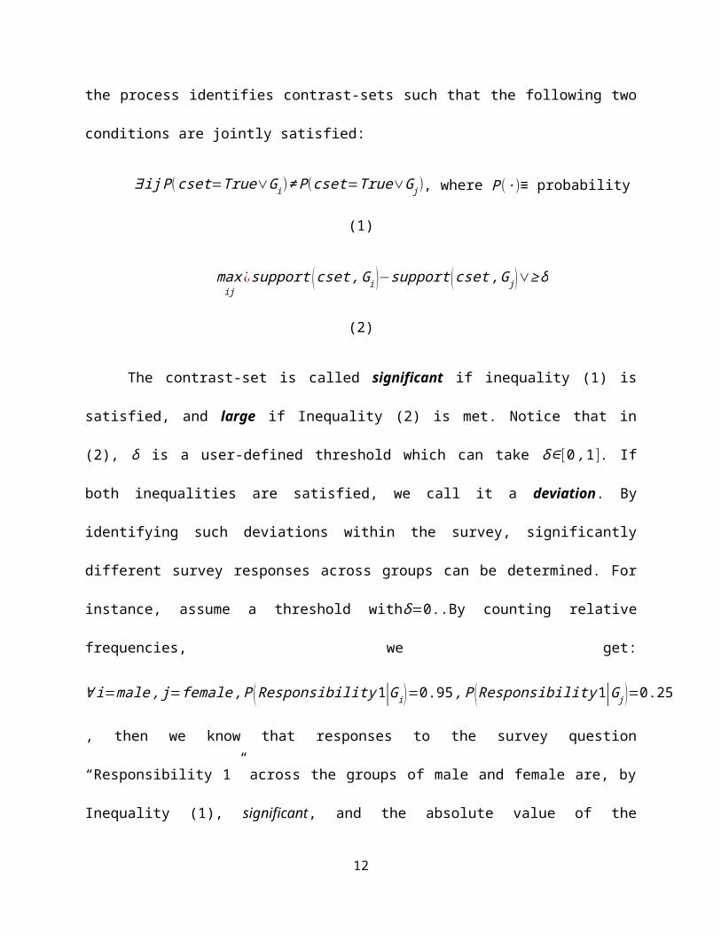
can be addressed. Mathematically, the process identifies contrast-sets such that the following two

conditions are jointly satisfied:

∃ ij P(cset=True∨Gi)≠ P(cset=True∨G j), where P(∙)≡ probability (1)

maxij

¿ support ( cset , Gi )−support (cset ,G j )∨≥ δ (2)

The contrast-set is called significant if inequality (1) is satisfied, and large if Inequality

(2) is met. Notice that in (2), δ is a user-defined threshold which can take δ∈[0 ,1]. If both

inequalities are satisfied, we call it a deviation. By identifying such deviations within the survey,

significantly different survey responses across groups can be determined. For instance, assume a

threshold withδ=0..By counting relative frequencies, we get:

∀ i=male , j=female , P ( Responsibility 1|Gi )=0.95 ,P ( Responsibility 1|G j )=0.25, then we know

that responses to the survey question “Responsibility 1” across the groups of male and female

are, by Inequality (1), significant, and the absolute value of the difference between their supports

is 0.7. Since this is larger than the threshold 0.5, it is deemed to be, by Inequality (2), large, and

therefore represents a deviation. Based on the sample probability distribution, this result

indicates that men and women answer this survey question differently. If the statistical

significance test is also met, this finding will imply that male and female respondents answered

the question significantly differently, and it is necessary to interview both households on

“responsibility 1”.

The method described above needs to be extended to account for the factor of the

presence of continuous, discrete or mixed variables in the dataset. Agricultural surveys include

mixes of categorical, ordinal and continuous data. Though ordinal data can be analyzed in the

same way as categorical data, continuous data may not be most accurately analyzed in this way.

8

Thus, this paper introduces an additional method, use of optimal bandwidth of Kernel density

estimates of continuous variables, to transform our continuous data into categorical form. This

method not only provides an approximation of the original probability distribution, but also

offers smoothness and continuity, which may better reduce information loss from this data

transformation. The kernel density estimators have the properties of smoothness, no end points

and the dependence on bandwidth rather than on width of bins, compared to the histogram

method (Duong 2001). The use of an optimal bandwidth in a kernel approach provides an

improved decision with respect to the optimal width of bins (the degree of approximation in a

histogram approach). The optimal bandwidth for the case of Gaussian distribution with a

Gaussian kernel (Zucchini 2003) is given by:

hopt=¿.

An Algorithm for Mining Contrast-sets:

In order to systematically detect contrast-sets, this paper employs an algorithm, STUCCO

(Search and Testing for Understandable Consistent Contrasts) (Bay and Pazzani 1999 and 2001),

it, in practice, works efficiently to mine numbers of potential candidates even at a low support

difference defined by Inequality (2) (Bay and Pazzani 1999). It also includes sub-algorithms for:

(i) statistical hypothesis testing for contrast-set validity, and (ii) control of Type I error to limit

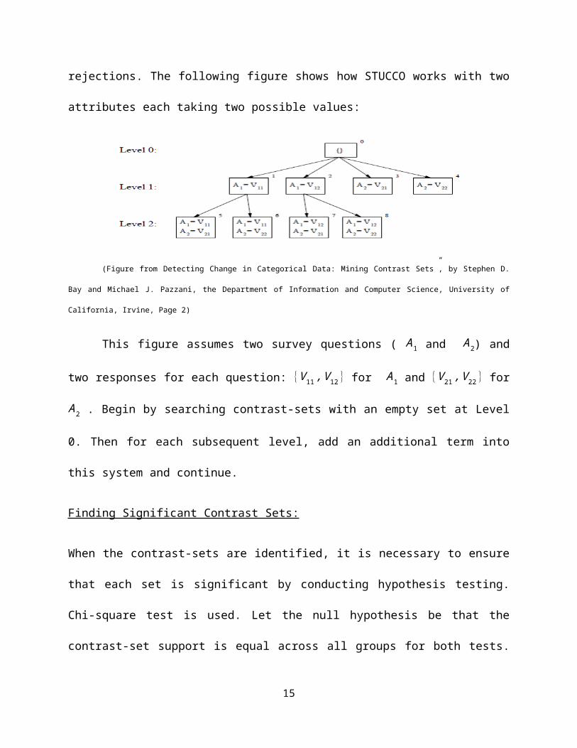
false rejections. The following figure shows how STUCCO works with two attributes each

taking two possible values:

9

(Figure from Detecting Change in Categorical Data: Mining Contrast Sets”, by Stephen D. Bay and Michael J. Pazzani, the

Department of Information and Computer Science, University of California, Irvine, Page 2)

This figure assumes two survey questions ( A1 and A2) and two responses for each

question: {V 11 ,V 12} for A1 and {V 21 ,V 22} for A2 . Begin by searching contrast-sets with an

empty set at Level 0. Then for each subsequent level, add an additional term into this system and

continue.

Finding Significant Contrast Sets:

When the contrast-sets are identified, it is necessary to ensure that each set is significant by

conducting hypothesis testing. Chi-square test is used. Let the null hypothesis be that the

contrast-set support is equal across all groups for both tests. Under these conditions, the support

can be conceived of as a form of frequency data which can be analyzed in contingency tables.

These tables include the truth of the contrast-set and the group membership.

Controlling Type I Error:

When testing a single hypothesis, the significance level sets the maximum probability of falsely

rejecting the null hypothesis. However, when conducting multiple hypothesis tests the

probability of false rejection can be high, and there still exists no optimal solution to address this

problem. One way to control Type I error in the case of multiple tests is to use a more stringent α

10

cutoff for the individual tests. Relate the α ilevels used for each individual test to a global α using

the following:

Bonferroni Inequality: Given any set of eventse1 ,e2 ,⋯ , en, the probability of their union

e1∪e2∪⋯∪en is less than or equal to the sum of the individual probabilities.

Simply, this inequality holds as long as: ∑i

αi ≤ α. Therefore, a different level of

significance can be used for each level in the searching process:

α l=min ( α2l / ¿Cl∨, αl−1)

where α l is a test cut-off for each level l , and ¿C l∨¿ is the total number of candidates at level l.

Comparison to Regression Analysis:

Very limited literature compares the method of mining contrast-sets and regression analysis. In

order to make this comparison, econometric models were estimated using a Multinomial Logistic

Model (MNL) to address the same issues examined by the contrast set methods. The measure by

Cameron and Trivedi 2005 is given with person j selecting one of given options i as:

P [ y j=i ]=P ji=exp (x i

' βi )∑ exp (x j

' βk ), where0<P ji<1

P [ y j=i ]=P ji ( β0+β1 x1+⋯+βk xk )=P ji ( β0+xβ ) , xβ=β0+β1 x1+⋯+βk xk

where: y j≡ the probability that the person j chooses option i (1≡ the interviewee, 2≡ your

spouse, 3≡ you and your spouse jointly responded), P [ y j=i ]; x j ≡ vector of variables in

contrasting groups of gender, for instance, Gender1=single male when comparing male and

11

female responses in this pair; β i ≡ vector of coefficients associated with the ithoption which

measures the effect across the pair of groups. To access the importance of characteristics and

other factors on household choices, again, six regression models are employed with MNL to

explain the impacts of the independent variables on the probability of choosing either a male, a

female, or both, for being in charge of those household activities. y j is still the probability for a

person j to choose option i, where option i is re-coded as 0 being only female, 1 only males and 2

both. Marginal effects are used for the interpretation of the models.

Data Analysis, Comparisons and Results:

The analysis on the survey responses by contrasting groups shows that the gender of the

respondent does have effects on certain survey responses. For subjective questions on who

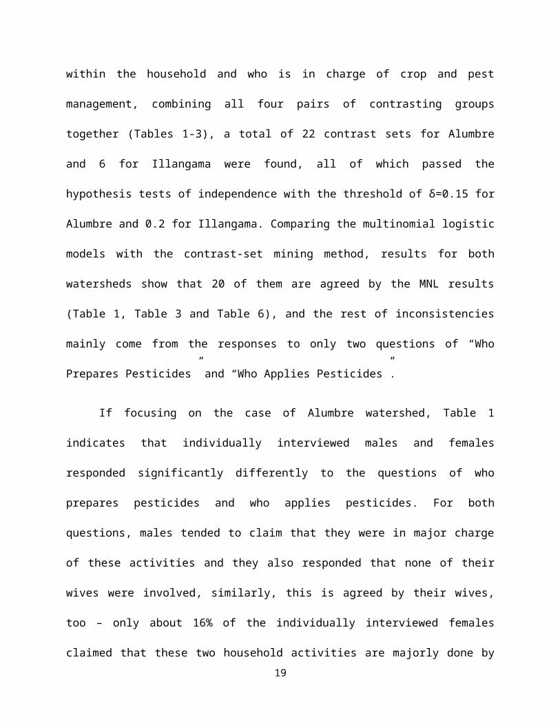
makes decisions within the household and who is in charge of crop and pest management,

combining all four pairs of contrasting groups together (Tables 1-3), a total of 22 contrast sets for

Alumbre and 6 for Illangama were found, all of which passed the hypothesis tests of

independence with the threshold of δ=0.15 for Alumbre and 0.2 for Illangama. Comparing the

multinomial logistic models with the contrast-set mining method, results for both watersheds

show that 20 of them are agreed by the MNL results (Table 1, Table 3 and Table 6), and the rest

of inconsistencies mainly come from the responses to only two questions of “Who Prepares

Pesticides” and “Who Applies Pesticides”.

If focusing on the case of Alumbre watershed, Table 1 indicates that individually

interviewed males and females responded significantly differently to the questions of who

prepares pesticides and who applies pesticides. For both questions, males tended to claim that

they were in major charge of these activities and they also responded that none of their wives

12

were involved, similarly, this is agreed by their wives, too – only about 16% of the individually

interviewed females claimed that these two household activities are majorly done by themselves

while roughly 50% of them still agreed that preparing and applying pesticides are their husbands’

roles. However, with the MNL models, Table 6 suggests that for these two survey questions,

though in the pure gender MNL models, the likelihood ratio test indicates that gender is

statistically significant at both 5% and 1% levels, it failed to deviate the responses to the

questions. Interestingly, if we compare Table 2 and Table 6, MNL model results agree perfectly

with the contrast-set results, and again, regarding the two questions of who prepares and who

applies pesticides, both of the two different methods clearly agreed that when males and females

were interviewed jointly but separately, both jointly surveyed males and females have the

agreement that these two are more men-related activities with both relatively large observed

frequencies or predicted probabilities. From this point, we can also conclude that, at least for

these two survey questions, when females are individually interviewed, they tended to claim that

the major responsibility are in their control while if the females were interviewed knowing that

their husbands were also to be interviewed, they tended to claim less self-responsibilities but

were more likely to claim that these were done majorly by males. And this can also be seen from

Table 6 in the contrasting groups between females and jointly interviewed females, that for both

of the questions, individually interviewed females were roughly 25% less likely to claim that

these were done by their husbands than jointly surveyed females. For the survey questions who

prepares pesticides and who applies pesticides, both contrast-set and MNL methods suggest that

when only one female is asked, she is more likely to claim her sole responsibility than jointly

interviewed females, and when both males and females were jointly interviewed, they made such

agreement that preparing and applying pesticides are more male-related tasks. In addition, the

13

contrast-set method itself also suggests that even males are females are individually interviewed,

they tended to both agree that these two activities are majorly done by males.

In the watershed of Illangama, these is another story for the two questions of who

preparing and applying pesticides: comparing the two methods (Table 3 and Table 6), results by

the contrast-set method show that when males and females are jointly interviewed, males are

much more likely to claim solely responsibility than females to the questions of who prepares

and applies pesticides, while with MNL models, such result was not found, thus MNL suggests

that regarding these two questions, jointly interviewed males and females did not responded

significantly differently, even though the likelihood ratio test shows that gender is a significant

variable in the models.

As we know, in fact, the Bonferroni inequality is generally conservative, and may

become especially conservative given a small sample size, such as 13 total observations for male

respondents in Illangama watershed in this study, and this may be one reason why contrast-set

mining method generally found less results than the MNL models – some potential contrast-set

candidates may be missed solely due to Bonferroni inequality, and because of the small sample,

the pre-defined thresholds may not work very well in defining how different two supports can

be, as, for example, a one data point change among the 13 male responses is relatively large.

Thus, what would the contrast-set result be if loosening the conservativeness of Bonferroni

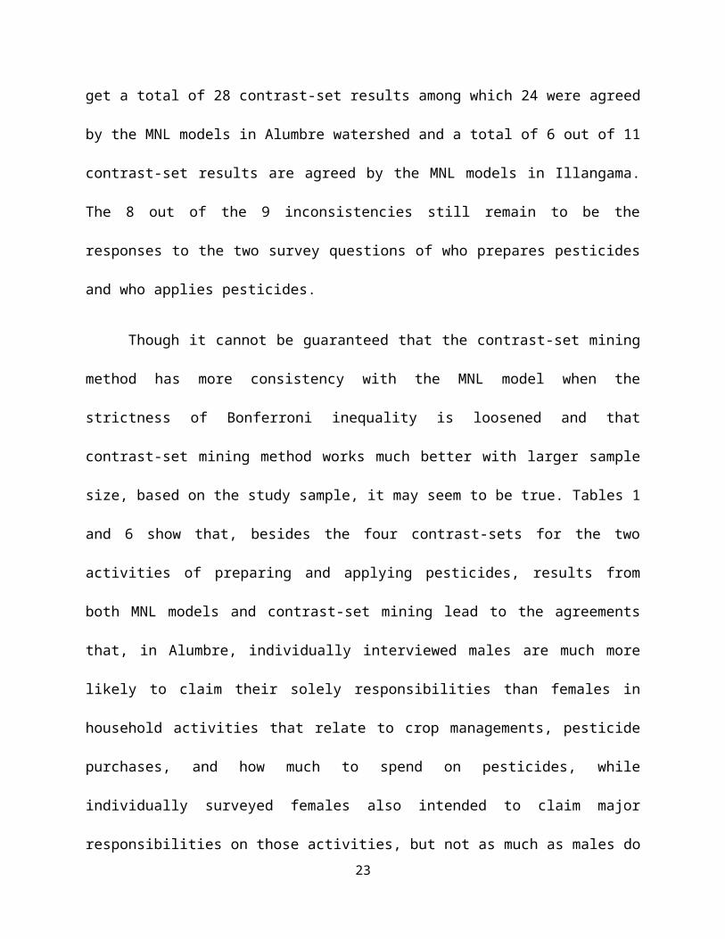
inequality? By requiring that each contrast-set may have a significance level no greater than a

tenth of alpha, which is a 0.005, then we would get a total of 28 contrast-set results among which

24 were agreed by the MNL models in Alumbre watershed and a total of 6 out of 11 contrast-set

results are agreed by the MNL models in Illangama. The 8 out of the 9 inconsistencies still

14

remain to be the responses to the two survey questions of who prepares pesticides and who

applies pesticides.

Though it cannot be guaranteed that the contrast-set mining method has more consistency

with the MNL model when the strictness of Bonferroni inequality is loosened and that contrast-

set mining method works much better with larger sample size, based on the study sample, it may

seem to be true. Tables 1 and 6 show that, besides the four contrast-sets for the two activities of

preparing and applying pesticides, results from both MNL models and contrast-set mining lead to

the agreements that, in Alumbre, individually interviewed males are much more likely to claim

their solely responsibilities than females in household activities that relate to crop managements,

pesticide purchases, and how much to spend on pesticides, while individually surveyed females

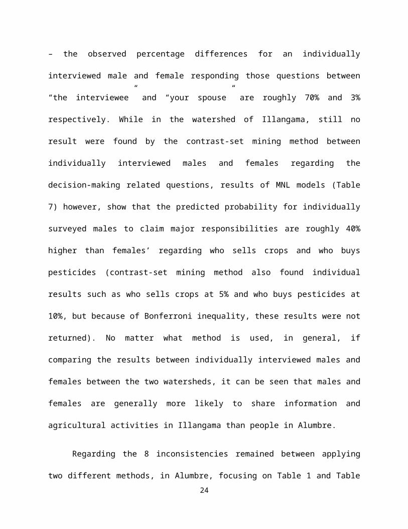
also intended to claim major responsibilities on those activities, but not as much as males do –

the observed percentage differences for an individually interviewed male and female responding

those questions between “the interviewee” and “your spouse” are roughly 70% and 3%

respectively. While in the watershed of Illangama, still no result were found by the contrast-set

mining method between individually interviewed males and females regarding the decision-

making related questions, results of MNL models (Table 7) however, show that the predicted

probability for individually surveyed males to claim major responsibilities are roughly 40%

higher than females’ regarding who sells crops and who buys pesticides (contrast-set mining

method also found individual results such as who sells crops at 5% and who buys pesticides at

10%, but because of Bonferroni inequality, these results were not returned). No matter what

method is used, in general, if comparing the results between individually interviewed males and

females between the two watersheds, it can be seen that males and females are generally more

likely to share information and agricultural activities in Illangama than people in Alumbre.

15

Regarding the 8 inconsistencies remained between applying two different methods, in

Alumbre, focusing on Table 1 and Table 6 for the contrasting groups of individually interviewed

males and females, results show that, in Table 1, contrast-set mining method returned the four

corresponding results because by its definition, the responses to the four options of the two

questions indeed differ “meaningfully” across the contrasting groups of individually surveyed

males and females based on the pre-defined threshold. However, if focusing on the column of

females’ observed frequencies, it can be clearly seen that, females subjectively think that they

take more responsibilities than their husbands though all the decision-making related questions

but who prepares pesticides and who applies pesticides – females themselves subjectively

affirmed that, regarding these two activities, their husbands are more likely to be in major

charge, thus, both individually interviewed males and females tend to agree that these two

activities are more male-related ones. Thus, even though the results and numbers shown in Table

1 and 6 indicate an inconsistency between the two methods, the analysis from both methods on

these two activities imply that both males and females tend to agree that these are majorly done

by males.

When comparing individually interviewed males and the males interviewed knowing that

their wives were also about to be surveyed, in Alumbre, both methods returned no results,

suggesting that within this pair of contrasting groups, individually interviewed and jointly

interviewed males did not respond to any of the survey questions significantly differently. While

in Illangama watershed, contrast-set mining method did not return any results, thus MNL model

cannot be used to check if there exists any inconsistency, but if only looking at Table 7, it can be

observed that individually interviewed males and jointly interviewed males responded differently

to only one question of who sells crops: there’s a 39% more chance for an individually

16

interviewed male to claim solely responsibility than jointly interviewed to this question and they

are less likely to select joint responsibility with their wives compared to jointly surveyed males.

It seems that, for both methods, on all the other five questions, it has been agreed that

individually interviewed males and jointly surveyed males do not have surprisingly different

answers.

To assess whether individually interviewed and jointly interviewed females responded to

the decision-making related questions differently in Illangama, Table 4 and 6 are used. With the

Bonferroni inequality imposed, no results were found by the contrast-set method, indicating that

females from this pair of contrasting groups did not respond to any of the survey questions

differently. However, Table 4 shows the contrast-set results when this restriction were loosened

to one tenth of alpha. For all of the results except for the question of who manages crops listed in

Table 4 found by the contrast-set mining method, MNL models have the corresponding perfect

matches with the contrast-set mining methods, with one additional finding: there is a 16% less

chance for individually interviewed females to respond joint responsibility with their husbands to

the question of who buys pesticides compared to the jointly interviewed women. In addition to

this point, Table 4 also shows that jointly interviewed females are more likely to claim joint

charge together with their husbands than individually surveyed females, and for the same

question, individually surveyed females tend to claim more responsibility. It can be seen that,

females are found to be likely to over-value their roles and participations in selling crops,

preparing and applying pesticides, and jointly surveyed females tend to claim joint

responsibilities. Moreover, it has been agreed by females that preparing and applying pesticides

are men-related tasks.

17

The last pair of contrasting groups consist of jointly interviewed males and jointly

interviewed females. To examine the gendered effects in these two groups, Table 2 and 6 are

referred for the watershed of Alumbre, and results show that for the total of 12 contrast-sets

discovered by contrast-set method, a 100% consistency is gained by the findings of MNL

models. Jointly interviewed males claimed sole responsibilities to all of the six decision-making

related survey questions and in general, jointly interviewed females intended to claim these

duties to be taken by their husbands, too, especially for who prepares pesticides and who applies

pesticides. In Illangama however, both methods agree that jointly interviewed males tend to

respond that they are in major charge of purchasing pesticides. Contrast-set mining method also

suggests that jointly interviewed males and females both tend to claim that the activities of

preparing and applying pesticides are mainly in charge by males, whereas by MNL models, there

is a bigger chance for jointly interviewed males to claim major responsibility in selling crops and

23% less chance to respond joint responsibility with their wives.

To respond to the issue of whether the gendered effects differ by household

characteristics and different type of questions, contrast-set methods mined no results, suggesting

that gender is the only factor to influence the farmers responding household decision-making

related questions differently, while both MNL model found that, for the questions of how much

to spend on pesticides, the importance of recommendation from the extension is a significant

factor to influence people’s decisions – both methods suggest that males who responded very

important to the question of how important is the recommendation by the extension are more

likely to claim that they are in major role of deciding how much money to be spent on

purchasing pesticides. In addition, MNL models also found that the ages of the respondents and

the distance from their houses to the roads are also the factors which may potentially affect

18

farmers, especially males to make household decisions such as in selling household crops,

purchasing pesticides, preparing pesticides and applying pesticides. Moreover, the hectares of

land own may potentially influence females in managing crops and males in deciding how much

to spend on pesticides. Even though these factors are found to be statistically significant at 5%

level, the corresponding coefficients are extremely small, and for the factor of importance of

recommendation by extension, MNL model indicates that with this factor, roughly 22% more

male farmers are more likely to take charge in deciding how much to spend on pesticides.

Conclusions:

The results of this paper provide a better understanding of intra household decision makings

involved in a potential program to offer training in agricultural management practices with a

focus on pest management practices in Ecuador, to address the general issue of does it matter

who we ask in the survey. The method of mining contrast-set is employed as the main measure in

this paper and multinomial logistic regression analysis is used for comparisons.

Findings suggest that generally, when only one respondent is interviewed, he or she is

more likely to claim major responsibility to certain subjective questions. In particular, males in

general tend to over-value their roles or involvements in household activities such as crop and

pesticide managements and under-value their wives’ participations regarding the subjective

survey questions that relate to farm household decision-making processes, and this situation

applies to either individually interviewed males or jointly interviewed males; females are found

to be likely to over-value their roles and participations in selling crops, preparing and applying

pesticides, and jointly surveyed females also tend to claim joint responsibilities. Even though

both males and females tend to claim major responsibilities in questions such as preparing and

19

applying pesticides in general, when only one female is asked, she is more likely to claim her

sole responsibility than jointly interviewed females, and when both males and females were

jointly interviewed, they made such agreement that preparing and applying pesticides are more

male-related tasks. In Alumbre, individually interviewed males are much more likely to claim

their solely responsibilities than females in household activities that relate to crop managements,

pesticide purchases, and how much to spend on pesticides, while individually surveyed females

also intended to claim major responsibilities on those activities, but not as much as males do.

Thus, on these such of survey questions, in order to obtain more accurate responses, it is

suggested that both males and females be interviewed.

Furthermore, upon the fact that none of the methods found such results to certain

objective/subjective questions that people in any assigned contrasting groups responded

significantly differently, thus, for such questions as crop productions, the importance of reduced

costs in purchasing pesticides, how important is the cost of IPM practices and the importance of

advices from neighbors, etc., females’ responses do not differ significantly with the males’ and

thus, one gender is adequate to be surveyed on such questions, no matter this female or male

respondent is individually surveyed or jointly surveyed. Meanwhile, for activities such as

purchasing, preparing and applying pesticides, crop management and deciding how much to

spend on pesticides, the individually interviewed males and jointly surveyed males do not have

surprisingly different responses in both watersheds, suggesting that if interviewing a male, either

individually or jointly surveyed male respondent may be enough for the survey, but this does not

necessarily mean that the male responses are reliable, and female responses are also need to be

taken.

20

Jointly interviewed males claimed sole responsibilities to all of the six decision-making

related survey questions and in general, jointly interviewed females intended to claim these

duties to be taken by their husbands, too, especially for who prepares pesticides and who applies

pesticides. In Illangama however, both methods agree that jointly interviewed males tend to

respond that they are in major charge of purchasing pesticides. Thus, compared to individually

interviewed respondents, jointly interviewed survey responses are relatively more reliable, but

more accuracy of the survey responses can be obtained by interview both jointly surveyed males

and females, while in Illangama, for the question of who purchasing pesticides, both jointly

interviewed males and females should be interviewed, but for other decision-making related

questions, one jointly interviewed gender is adequate to survey.

Nevertheless, the participations by females in activities which relate to pesticide

management cannot be neglected, and thus more accuracy may be gained by asking both male

and female about this type of question on a survey, such as who decides how much money to

spend on purchasing pesticides and who is charge of managing crops.

Pattern of household decision making and gender responsibility differ by different

watershed – gendered impact on decision-making related questions and pesticide expenditures

are more balanced in Illannaga than those in Allumbre, which may also imply that males from

Allumbre tend to weigh more gender roles on themselves than the ones in Illannaga. Thus, in

Illangama, regarding those survey questions, one gender is generally enough to be interviewed.

(This is not a final paper.)

21

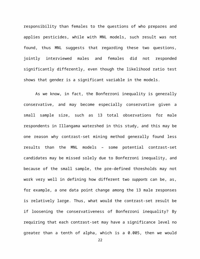
Table 1. Level One Contrast Sets, Alumbre

Contrast Sets (δ = 0.15)Contrasting Groups P-values

(α = 0.05)Male FemaleWho Manages Crops = Interviewee 74.36% 30.85% <0.0001Who Manages Crops = Your Spouse 1.28% 27.66% <0.0001How Much to Spend on Pesticides = Interviewee 69.23% 30.85% <0.0001How Much to Spend on Pesticides = Your Spouse 3.85% 27.66% <0.0001Who Buys Pesticides = Interviewee 75.64% 34.04% <0.0001Who Buys Pesticides = Your Spouse 2.56% 30.85% <0.0001Who Prepares Pesticides = Interviewee 75.64% 15.96% <0.0001Who Prepares Pesticides = Your Spouse 0.00% 52.13% <0.0001Who Applies Pesticides = Interviewee 71.79% 15.96% <0.0001Who Applies Pesticides = Your Spouse 0.00% 48.94% <0.0001

Loosing Bonferroni Inequality at α/10Who Sells Crops = Interviewee 61.54% 37.23% 0.001Who Sells Crops = Your Spouse 5.13% 24.47% 0.001

Table 2. Level One Contrast Sets, Alumbre


(α = 0.05)Joint Male Joint Female

Who Sells Crops = Interviewee 45.59% 17.65% < 0.0001Who Sells Crops = Your Spouse 5.88% 23.53% < 0.0001Who Manages Crops = Interviewee 58.82% 19.12% < 0.0001Who Manages Crops = Your Spouse 7.35% 38.24% < 0.0001How Much to Spend on Pesticides = Interviewee 52.94% 17.65% < 0.0001How Much to Spend on Pesticides = Your Spouse 8.82% 41.18% < 0.0001Who Buys Pesticides = Interviewee 66.18% 22.06% < 0.0001Who Buys Pesticides = Your Spouse 7.35% 36.76% < 0.0001Who Prepares Pesticides = Interviewee 86.76% 13.24% < 0.0001Who Prepares Pesticides = Your Spouse 2.94% 73.53% < 0.0001Who Applies Pesticides = Interviewee 80.88% 14.71% < 0.0001Who Applies Pesticides = Your Spouse 4.41% 73.53% < 0.0001

Table 3. Level One Contrast Sets, IllangamaContrast Sets (δ = 0.2) Contrasting Groups P-values

22

(α = 0.05)Joint Male Joint Female

Who Buys Pesticides = Interviewee 66.67% 6.90% < 0.0001Who Buys Pesticides = Your Spouse 3.33% 55.17% < 0.0001Who Prepares Pesticides = Interviewee 96.55% 10.34% < 0.0001Who Prepares Pesticides = Your Spouse 0.00% 86.21% < 0.0001Who Applies Pesticides = Interviewee 96.55% 10.34% < 0.0001Who Applies Pesticides = Your Spouse 0.00% 86.21% < 0.0001

Table 4. Level One Contrast Sets for AlumbreLoosening Bonferroni Inequality at α/10


(α = 0.05)Female Joint Female

Who Sells Crops = Interviewee 37.23% 17.65% 0.001Who Sells Crops = Jointly 28.72% 57.35% 0.001Who Prepares Pesticides = Your Spouse 52.13% 73.53% 0.003Who Applies Pesticides = Your Spouse 48.94% 73.53% 0.001

Table 5. Level One Contrast Sets for Illangama (Female vs. Joint Female)Loosing Bonferroni Inequality at α/10


(α = 0.05)Female Joint Female

Who Manages Crops = Interviewee 32.35% 0.00% 0.003Who Prepares Pesticides = Interviewee 43.75% 10.34% 0.003Who Prepares Pesticides = Your Spouse 46.88% 86.21% 0.003Who Applies Pesticides = Interviewee 46.88% 10.34% 0.002Who Applies Pesticides = Your Spouse 43.75% 86.21% 0.002

23

dy/dx LR P>chi2 P>|Z| dy/dx LR P>chi2 P>|Z| dy/dx LR P>chi2 P>|Z| dy/dx LR P>chi2 P>|Z|The interviwee 0.2419 <0.0001 0.1529 0.05 0.1755 0.0120 0.264 < 0.0001

Your spouse -0.2159 0.0010 -0.0074 0.8370 -0.0062 0.9230 -0.1788 0.0070You and your spouse -0.0012 0.9860 -0.1811 0.0120 -0.2715 < .0001 -0.0986 0.247

dy/dx LR P>chi2 P>|Z| dy/dx LR P>chi2 P>|Z| dy/dx LR P>chi2 P>|Z| dy/dx LR P>chi2 P>|Z|The interviwee 0.4162 < 0.0001 0.1565 0.036 0.1159 0.0960 0.3511 < 0.0001

Your spouse -0.3584 0.0020 -0.0688 0.1530 -0.1049 0.1380 -0.2939 < 0.0001You and your spouse 0.0067 0.9170 -0.0828 0.2300 -0.0771 0.2760 -0.0359 0.6150


Your spouse -0.2567 0.0010 -0.0497 0.245 -0.1342 0.0540 -0.3062 < 0.0001You and your spouse -0.0024 0.9690 -0.1061 0.1440 -0.0836 0.2380 -0.0017 0.9820


Your spouse -0.3245 < 0.0001 -0.0495 0.229 -0.0652 0.3640 -0.2745 < 0.0001You and your spouse 0.0326 0.5230 -0.0272 0.6800 -0.1597 0.0120 -0.1062 0.1180

dy/dx LR P>chi2 P>|Z| dy/dx LR P>chi2 P>|Z| dy/dx LR P>chi2 P>|Z| dy/dx LR P>chi2 P>|Z|The interviwee 1.0505 0.9770 0.0048 1.0000 0.0119 0.8230 0.4269 < 0.0001

Your spouse -2.3800 0.9830 -0.2035 0.9920 -0.2390 0.0020 -0.4618 < 0.0001You and your spouse 0.2505 0.9870 -0.0344 0.9820 -0.0276 0.4610 0.0246 0.2470

dy/dx LR P>chi2 P>|Z| dy/dx LR P>chi2 P>|Z| dy/dx LR P>chi2 P>|Z| dy/dx LR P>chi2 P>|Z|The interviwee 1.004 0.9770 0.1107 0.9960 -0.0059 0.9110 0.4258 < 0.0001

Your spouse -2.3764 0.9830 -0.3014 0.9900 -0.2722 < 0.0001 -0.4660 < 0.0001You and your spouse 0.2418 0.9860 -0.0244 0.9910 -0.0157 0.6550 0.0238 0.2120

Joint Male vs. Joint FemaleGender=1 if Joint Male; 0 Joint Female

< 0.0001


< 0.0001


< 0.0001


< 0.0001


< 0.0001


0.0010

Table 6. Pure Gendered Marginal Effects on Six Decision-Making Questions with MNL Models, Alumbre

Female vs. Joint FemaleGender=1 if Female; 0 Joint Female

< 0.0001


0.0010


0.0120


0.0290


0.1200


< 0.0001

Male vs. Joint MaleGender=1 if Male; 0 Joint Male


0.209


0.112


0.099

0.002


0.001


0.434

VariablesMale vs. Female

Gender=1 if Male; 0 Female

Who Sells Crops

0.001



Who Manages

Crops< 0.0001



How Much to Spend on Pesticides

< 0.0001



Who Buys Pesticides

< 0.0001



Who Prepares

Pesticides< 0.0001



Who Applies Pesticides

< 0.0001

dy/dx LR P>chi2 P>|Z| dy/dx LR P>chi2 P>|Z| dy/dx LR P>chi2 P>|Z| dy/dx LR P>chi2 P>|Z|The Interviewee 0.3995 < 0.0001 0.3853 0.002 0.2381 0.0220 0.2659 0.0090

Your spouse -0.098 0.4920 -0.0036 0.9680 0.049 0.5740 -0.0338 0.6570You and your spouse -0.3016 0.0680 -0.3817 0.0080 -0.2870 0.004 -0.2321 0.04

dy/dx LR P>chi2 P>|Z| dy/dx LR P>chi2 P>|Z| dy/dx LR P>chi2 P>|Z| dy/dx LR P>chi2 P>|Z|The Interviewee 1.1616 0.992 0.1481 0.364 2.0414 0.9910 2.2813 0.9940

Your spouse -2.3810 0.9930 − − -0.8174 0.9910 -2.1712 0.9940You and your spouse 1.2194 0.9940 -0.1481 0.3640 -1.2240 0.9910 -0.1099 1.0000

dy/dx LR P>chi2 P>|Z| dy/dx LR P>chi2 P>|Z| dy/dx LR P>chi2 P>|Z| dy/dx LR P>chi2 P>|Z|The Interviewee 0.9154 0.986 0.4282 0.973 1.9300 0.9910 1.4782 0.9900

Your spouse -1.8280 0.9900 -0.3274 0.995 -0.5787 0.9910 -0.3426 0.9460You and your spouse 0.9125 0.9920 -0.1008 0.9980 -1.3514 0.9910 -1.1356 0.9920

dy/dx LR P>chi2 P>|Z| dy/dx LR P>chi2 P>|Z| dy/dx LR P>chi2 P>|Z| dy/dx LR P>chi2 P>|Z|The Interviewee 0.3863 0.003 0.0991 0.557 0.2964 0.0080 0.4390 < 0.0001

Your spouse -0.2928 0.13 0.0436 0.524 -0.2138 0.0510 -0.4299 < 0.0001You and your spouse -0.0936 0.5730 -0.1427 0.3750 -0.0826 0.4610 -0.0091 0.9360

dy/dx LR P>chi2 P>|Z| dy/dx LR P>chi2 P>|Z| dy/dx LR P>chi2 P>|Z| dy/dx LR P>chi2 P>|Z|The Interviewee 0.7911 0.9890 -0.3206 0.9990 0.3179 0.0010 1.0471 0.9960

Your spouse 0.1182 0.9980 0.7089 0.9950 -0.3675 < 0.0001 -1.3081 0.9970You and your spouse -0.9093 0.9940 -0.3883 0.9980 0.0496 0.4490 0.2610 0.9970

dy/dx LR P>chi2 P>|Z| dy/dx LR P>chi2 P>|Z| dy/dx LR P>chi2 P>|Z| dy/dx LR P>chi2 P>|Z|The Interviewee 0.7961 0.9890 -0.3206 0.9990 0.3410 < 0.0001 1.0471 0.9960

Your spouse 0.1152 0.9980 0.7089 0.9950 -0.3882 < 0.0001 -1.3081 0.9970You and your spouse -0.9112 0.9940 -0.3883 0.9980 0.0472 0.4600 0.2610 0.9970

Gender1=1 if Male; 0 Female

0.022

Male vs. FemaleGender1=1 if Male; 0 Female

Male vs. Female


Gender1=1 if Male; 0 Female

Who Sells Crops

0.023


Who Manages

Crops0.033

Gender1=1 if Male; 0 Joint MaleMale vs. Joint Male

0.037


0.036

Who Prepares

Pesticides0.024


Who Buys Pesticides

0.039



0.0310


0.062


0.062


0.569


0.027


0.379

Gender2=1 if Female; 0 Joint Female

0.0020

Female vs. Joint FemaleGender2=1 if Female; 0 Joint Female

0.0040

< 0.0001

Joint Male vs. Joint FemaleGender2=1 if Joint Male; 0 Joint Female

0.0440

Female vs. Joint Female


0.0190


0.0010


< 0.0001


Table 7. Pure Gendered Marginal Effects on Six Decision-Making Questions with MNL Models, Illangama

" − " indicates zero observation.


< 0.0001


< 0.0001


< 0.0001


< 0.0001


24

dy/dx P > |Z| dy/dx P > |Z| dy/dx P > |Z|Age Age of the interviewee (years) 0.009 0.0006 0.6990 0.0058 0.0010 -0.0055 0.0040Edu Years of education (years) 0.021 0.0047 0.4110 0.0080 0.2750 -0.0199 0.0100Distance Meters from house to road 0.028 0.0000 0.4230 0.0000 0.0110 0.0000 0.2620ImpRec3 1 = Very important: recommendation from extension 0.016 -0.0762 0.0820 0.0595 0.2780 0.0838 0.1330ACurva1 1 = Applies contour practicing 0.029 -1.8300 0.9930 1.3579 0.9890 1.1062 0.9910FWorker Number of female workers in farm 0.462HaProd Hectares of land available for production 0.424HaOwn Hectares of land own 0.297NotAware3 1 = Very important: informed of IPM practices 0.461ImpSale2 1 = somewhat important: recommendation by pest dealers 0.731Krotation 1 = Knows crop rotation 0.730Arotation 1 = Applies crop rotation 0.863Irrigation 1=Household has access to an irrigation system 0.078Kcurva 1= Knows contour practicing 0.210

dy/dx P > |Z| dy/dx P > |Z| dy/dx P > |Z|HaOwn Hectares of land own 0.041 -0.0255 0.0180 0.0234 0.0630 -0.0067 0.5560Age Age of the interviewee (years) 0.232Edu Years of education (years) 0.618Distance Meters from house to road 0.194FWorker Number of female workers in farm 0.312HaProd Hectares of land available for production 0.421ImpRec3 1 = Very important: recommendation from extension 0.256NotAware3 1 = Very important: informed of IPM practices 0.141ImpSale2 1 = somewhat important: recommendation by pest dealers 0.443KRotation1 1 = Knows crop rotation 0.242ARotation1 1 = Applies crop rotation 0.308Irrigation1 1=Household has access to an irrigation system 0.222KCurva1 1= Knows contour practicing 0.669ACurva1 1 = Applies contour practicing 0.130

dy/dx P > |Z| dy/dx P > |Z| dy/dx P > |Z|FWorker Number of female workers in farm 0.040 -0.0048 0.8200 -0.0310 0.1510 0.0011 0.9590HaProd Hectares of land available for production 0.041 -0.0098 0.4480 0.0236 0.0440 0.0102 0.3510ImpRec3 1 = Very important: recommendation from extension 0.001 -0.0709 0.0910 0.2154 < 0.0001 -0.0970 0.0640Age Age of the interviewee (years) 0.118Edu Years of education (years) 0.819Distance Meters from house to road 0.133HaOwn Hectares of land own 0.881NotAware3 1 = Very important: informed of IPM practices 0.404ImpSale2 1 = somewhat important: recommendation by pest dealers 0.423KRotation1 1 = Knows crop rotation 0.794ARotation1 1 = Applies crop rotation 0.895Irrigation1 1=Household has access to an irrigation system 0.789KCurva1 1= Knows contour practicing 0.946ACurva1 1 = Applies contour practicing 0.549

Female Male

P>chi2

Table 8. Gendered Marginal Effect Differences by Type of Question and Household Characteristics, Alumbre

Female Male Joint

Statistically Insignificant at 5% by Likelihood Ratio Test

Variables Variable Discriptions

Variables Variable DiscriptionsP>chi2

Variables Variable Discriptions Female Male Joint


Who Sells Crops

Who Manages Crops


P>chi2

Joint


25

Table 8. Continued:

dy/dx P > |Z| dy/dx P > |Z| dy/dx P > |Z|Age Age of the interviewee (years) 0.009 0.00060 0.69900 0.00580 0.00100 -0.00550 0.00400Edu Years of education (years) 0.021 0.00470 0.41100 0.00800 0.27500 -0.01990 0.01000Distance Meters from house to road 0.028 0.00001 0.42300 0.00003 0.01100 -0.00002 0.26200ImpRec3 1 = Very important: recommendation from extension 0.016 -0.07620 0.08200 0.00003 0.01100 -0.00002 0.26200ACurva1 1 = Applies contour practicing 0.029 -1.83000 0.99300 1.35790 0.98900 1.10620 0.99100FWorker Number of female workers in farm 0.462HaProd Hectares of land available for production 0.424HaOwn Hectares of land own 0.297NotAware3 1 = Very important: informed of IPM practices 0.461ImpSale2 1 = somewhat important: recommendation by pest dealers 0.731KRotation1 1 = Knows crop rotation 0.730ARotation1 1 = Applies crop rotation 0.863Irrigation1 1=Household has access to an irrigation system 0.078KCurva1 1= Knows contour practicing 0.210

dy/dx P > |Z| dy/dx P > |Z| dy/dx P > |Z|Age Age of the interviewee (years) 0.009 0.00060 0.69900 0.00580 0.00100 -0.00550 0.00400Edu Years of education (years) 0.021 0.00470 0.41100 0.00800 0.27500 -0.01990 0.01000Distance Meters from house to road 0.028 0.00001 0.42300 0.00003 0.01100 -0.00002 0.26200ImpRec3 1 = Very important: recommendation from extension 0.016 -0.07620 0.08200 0.05950 0.27800 0.08380 0.13300ACurva1 1 = Applies contour practicing 0.029 -1.83000 0.99300 1.35790 0.98900 1.10620 0.99100FWorker Number of female workers in farm 0.462HaProd Hectares of land available for production 0.424HaOwn Hectares of land own 0.297NotAware3 1 = Very important: informed of IPM practices 0.461ImpSale2 1 = somewhat important: recommendation by pest dealers 0.731KRotation1 1 = Knows crop rotation 0.730ARotation1 1 = Applies crop rotation 0.863Irrigation1 1=Household has access to an irrigation system 0.078KCurva1 1= Knows contour practicing 0.210

dy/dx P > |Z| dy/dx P > |Z| dy/dx P > |Z|Age Age of the interviewee (years) 0.009 0.00060 0.69900 0.00580 0.00100 -0.00550 0.00400Edu Years of education (years) 0.021 0.00470 0.41100 0.00800 0.27500 -0.01980 0.01000Distance Meters from house to road 0.028 0.00001 0.42300 0.00003 0.01100 -0.00002 0.26200ImpRec3 1 = Very important: recommendation from extension 0.016 -0.07620 0.08200 0.05950 0.27800 0.08380 0.13300ACurva1 1 = Applies contour practicing 0.029 -1.83000 0.99300 1.35790 0.98900 1.10620 0.99100FWorker Number of female workers in farm 0.462HaProd Hectares of land available for production 0.424HaOwn Hectares of land own 0.297NotAware3 1 = Very important: informed of IPM practices 0.461ImpSale2 1 = somewhat important: recommendation by pest dealers 0.731KRotation1 1 = Knows crop rotation 0.730ARotation1 1 = Applies crop rotation 0.863Irrigation1 1=Household has access to an irrigation system 0.078KCurva1 1= Knows contour practicing 0.210







P>chi2

Who Buys Pesticides

P>chi2

Who Prepares Pesticides

P>chi2


26

dy/dx P > |Z| dy/dx P > |Z| dy/dx P > |Z|Age Age of the interviewee (years) 0.949Edu Years of education (years) 0.854Distance Meters from house to road 0.102FWorker Number of female workers in farm 0.891HaProd Hectares of land available for production 0.376HaOwn Hectares of land own 0.986ImpTech3 3 = Very important: technical advices 0.348NotAware3 3 = Very important: informed of IPM practices 0.784Irrigation1 1=Household has access to an irrigation system 0.546ExtVisit1 1 = Visited by extension 0.299KCurva1 1= Knows contour practicing 0.676ACurva1 1 = Applies contour practicing 0.766ImpSale2 2 = somewhat important: recommendation by pest dealers 0.518


dy/dx P > |Z| dy/dx P > |Z| dy/dx P > |Z|KCurva1 1= Knows contour practicing 0.041 -0.9605 0.9980 -2.5611 0.9960 3.5215 0.9940Age Age of the interviewee (years) 0.973Edu Years of education (years) 0.861Distance Meters from house to road 0.543FWorker Number of female workers in farm 0.266HaProd Hectares of land available for production 0.789HaOwn Hectares of land own 0.990ImpTech3 3 = Very important: technical advices 0.956NotAware3 3 = Very important: informed of IPM practices 0.850Irrigation1 1=Household has access to an irrigation system 0.810ExtVisit1 1 = Visited by extension 0.862ACurva1 1 = Applies contour practicing 0.358ImpSale2 2 = somewhat important: recommendation by pest dealers 0.999

Table 9. Gendered Marginal Effect Differences by Type of Question and Household Characteristics, Illangama

Variables Variable Discriptions Female Male JointWho Sells Crops

P>chi2


Variables Variable Discriptions Female Male JointP>chi2




Who Manages Crops

P>chi2


27

Table 9. Continued:




Variables Variable Discriptions Female Male JointP>chi2

Who Buys Pesticides

Variables Variable Discriptions Female Male JointWho Prepares Pesticides

P>chi2

Variables Variable Discriptions Female Male JointWho Applies Pesticides

P>chi2




28

References:

1. Thangata, P.H., Hildebrand, P.E., and C.H. Gladwin, 2002. Modeling Agroforestry Adoption and Household Decision Making in Malawi. African Studies Quarterly, The Online Journal for African Studies. http://asq.africa.ufl.edu/v6/v6i1a11.htm. Accessed 03/21/14.

2. Min Bdr. Gurung and Brigitte Leduc, November 2009. Guidelines for a Gender Sensitive Participatory Approach. International Centre for Integrated Mountain Development (ICIMOD). Electronic pdf file.

3. Victor Hugo Barrera, Luis Orlando Escudero, Jeffrey Alwang, Robert Andrade, May 2012. Integrated Management of Natural Resources in the Ecuador Highlands. Agricultural Sciences, Vol.3, No.5, 768-779 (2012). http://dx.doi.org/10.4236/as.2012.35093. Accessed 03/21/14.

4. Elena Bardasi, Kathleen Beegle, Andrew Dillon, Pieter Serneels, 2010. Do Labor Statistics Depend on How and to Whom the Questions Are Asked? Results from a Survey Experiment in Tanzania. Policy Research Working Paper 5192. The World Bank, Development Research Group, Poverty and Inequality Team. http://elibrary.worldbank.org/doi/pdf/10.1596/1813-9450-5192.

5. Proxy Reporting in the Consumer Expenditure Surveys Program. First Workshop of the Consumer Expenditure Surveys Redesign Paper, Proxy Reporting. Bureau of Labor Statistics. http://www.bls.gov/cex/methwrkshpproxyrpting.pdf. Accessed 03/20/14.

6. Alexander Todorov, 2003. Cognitive Procedures for Correcting Proxy-response Biases in Surveys. Page 215 Summary, Page 222. Applied Cognitive Psychology. Appl.Cognit.Psychol. 17: 215-224 (2003). Published online in Wiley InterScience 28 November 2002. DOI: 10.1002/acp.850.

7. Gerry E. Hendershot, 2004. The Effects of Survey Nonresponse and Proxy Response on Measures of Employment for Persons with Disabilities. Disability Studies Quarterly. Spring 2004, Vol.24, No.2. http://dsq-sds.org/article/view/481/658. Cited from Abstract.

8. Monica Fisher, Jeffrey J. Reimer, Edward R. Carr, 2010. Who Should be Interviewed in Surveys of Household Income? Development Strategy and Governance Division. IFPRI Discussion Paper 00949. International Food Policy Research Institute. http://www.ifpri.org/sites/default/files/publications/ifpridp00949.pdf.

9. Steven Buck and Jeffrey Alwang, 2010. Agricultural Extension, Trust and Learning: Results from Economic Experiments in Ecuador. Agricultural Economics, Vol.42, Issue 6. First published online: DOI: 10.1111/j.1574-0862.2011.00547.x. Wiley Online Library.

10. Kellyn Paige Montgomery, 2011. Spatial and Gender Dimensions of IPM Adoption in Uganda. http://scholar.lib.vt.edu/theses/available/etd-06132011-192329/unrestricted/Montgomery_KP_T_2011.pdf.

11. Kalton, G., and H. Schuman, 1982. The Effect of the Question on Survey Responses: A Review. Journal of the Royal Statistical Society, Vol.145, No.1

12. Jacques Charmes 1998. Women Working in the Informal Sector in Africa: New Methods and New Data. Paper prepared for the United Nations Statistics Division, the Gender and

29

Development Programme of the United Nations Development Programme (UNDP) and project "Women in Informal Employment: Globalizing and Organizing" (WIEGO). An earlier version was presented at the Delhi Group Meeting on Informal Sector Statistics, 1998. United Nations Statistics Division. http://unstats.un.org/unsd/methods/timeuse/infresource_papers/charmes_informal_1.htm.

13. Carmen Diana Deere, 2005. The Feminization of Agriculture? Economic Restructuring in Rural Latin America. United National Research Institute for Social Development. Occasional paper 1.

14. Lawrie Mott, David Fore, Jennifer Curtis, Gina Solomon, 1997. Our Children at Risk: the Five Worst Environmental Threats to Their Health. Chapter 5: Pesticides. Natural Resources Defense Council. http://www.nrdc.org/health/kids/ocar/ocarinx.asp. Accessed 03/23/14.

15. Cole D.C., Sherwood S., Crissman C., Barrera V., Espinosa P., 2002. Pesticides and Health in Highland Ecuadorian Potato Production: Assessing Impacts and Developing Responses. Int J Occup Environ Health 2002, 8:182-190.

16. Ecuador Fair Trade Visit Part I: Adventures in Organic Fair Trade Alcohol. Fair World Project. http://fairworldproject.org/blogs/ecuador-fair-trade-visit-part-i-adventures-in-organic-alcohol/. Accessed 3/21/14.

17. Investment Brief: Ecuador, 2012. Texal Association. Cited from “Social Challenges” section. http://www.nesst.org/wp-content/uploads/2012/07/2012-Ecuador-Texal-EN.pdf. Accessed 03/26/14.

18. Crop Biodiversity, to Reduce Pest and Disease Damage, Ecuador. http://agrobiodiversityplatform.org/cropbiodiversity/the-countries/the-americas/ecuador/. Accessed 03/22/14.

19. Bay, S. D. and Pazzani, M. J., 1999. Detecting Change in Categorical Data: Mining Contrast Sets. In Proceedings of the Fifth International Conference on Knowledge Discovery and Data Mining.

20. Bay, S. D. and Pazzani, M. J., 2001. Detecting Group Differences: Mining Contrast Sets. Data Mining and Knowledge Discovery. Vol.5, No.3 213-246.

21. Walter Zucchini, 2003. Applied Smoothing Techniques, Part I: Kernel Density Estimation, Page 15-19.

22. Tarn Duong, 2001. An Introduction to Kernel Density Estimation. http://www.mvstat.net/tduong/research/seminars/seminar-2001-05/. Accessed 3/25/14.

23. Bruce Weaver, 2013. Assumptions/Restrictions for Chi-square Tests on Contingency Tables. LakeheadUniversity.https://sites.google.com/a/lakeheadu.ca/bweaver/Home/statistics/notes/chisqr_assumptions. Accessed 3/24/14.

24. McDonald, J. H., 2009. Fisher’s Exact Test of Independence, Handbook of Biological Statistics, http://udel.edu/~mcdonald/statfishers.html. Accessed 3/24/14.

25. A.Colin Cameron and Pravin K.Trivedi, 2005. Microeconometrics: Methods and Applications, Cambridge University Press, New York

26. Agrawal. R., Imielinski, T., and Swami, A.N. 1993. Mining Association Rules between Sets of Items in Large DataBases, In Proceedings of the 1993 ACM SIGMOD International

30

Conference on Management of Data, P. Buneman and S. Jajodia, Eds. Washington, D.C., 207-216

27. Sergio A. Alvarez, 2003. Chi-squared Computation for Association Rules: Preliminary Results. Technical Report BC-CS-2003-01

28. Association Rule Mining: Applications in Various Areas, by Akash Rajak and Mahendra Kumar Gupta, Krishna Institute of Engineering & Technology, Page 1

29. A Survey of Association Rules, by Margaret H. Dunham, Yongqiao Xiao, Department of Computer Science and Engineering, Southern Methodist University, Le Gruenwald, Zahid Hossain, Department of Computer Science, University of Oklahoma, Page 2

31

ageconsearch.umn.eduageconsearch.umn.edu/record/170634/files/gendered effects... · web...

Documents