efficiency of tidal turbine farms
TRANSCRIPT
8132019 Efficiency of Tidal Turbine Farms
httpslidepdfcomreaderfullefficiency-of-tidal-turbine-farms 18
Realizing the potential of tidal currents and the ef 1047297ciency of turbine farms
in a channel
Ross Vennell
Ocean Physics Group Department of Marine Science University of Otago 310 Castle St Dunedin 9054 New Zealand
a r t i c l e i n f o
Article history
Received 2 December 2010
Accepted 29 March 2012
Available online 11 May 2012
Keywords
Tidal stream power
Tidal turbine
Farm ef 1047297ciency
Power from tidal channels
a b s t r a c t
Tidal turbines in strong 1047298
ows have the potential to produce signi1047297
cant power However not all of thispotential can be realized when gaps between turbines are required to allow navigation along a channel A
review of recent works is used to estimate the scale of farm required to realize a signi 1047297cant fraction of
a channelrsquos potential These works provide the 1047297rst physically coherent approach to estimating the
maximum power output from a given number of turbines in a channel The fraction of the potential
realizable from a number of turbines a farmrsquos 1047298uid dynamic ef 1047297ciency is constrained by how much of
the channelrsquos cross-section the turbines are permitted to occupy and an environmentally acceptable 1047298ow
speed reduction Farm ef 1047297ciency increases as optimally tuned turbines are added to its cross-section
while output per turbine increases in tidal straits and decreases in shallow channels Adding rows of
optimally tuned turbines also increases farm ef 1047297ciency but with a diminishing return on additional rows
The diminishing return and 1047298ow reduction are strongly in1047298uenced by how much of the cross-section can
be occupied and the dynamical balance of the undisturbed channel Estimates for two example channels
show that realizing much of the MW potential of shallow channels may well be possible with existing
turbines However unless high blockage ratios are possible it will be more dif 1047297cult to realize the pro-
portionately larger potential of tidal straits until larger turbines with a lower optimum operating velocity
are developed
2012 Elsevier Ltd All rights reserved
1 Introduction
Underwater turbines in strong tidal currents can contribute to
the need for renewable energy sources To make a signi1047297cant
contribution many turbines must be grouped into large tidal farms
to exploit the energy of high 1047298ows through narrow tidal channels
This leads to a critical question how does power production scale
as a turbine farm expands from a single turbine into a large energy
farm While adding turbines to a farm increases its generation
capacity power extraction also enhances drag on the1047298owalong thechannel This enhanced drag slows 1047298ows along the channel
reducing power production by all turbines Flow reduction
becomes more signi1047297cant as a farm grows and ultimately limits
a channelrsquos potential to produce power ([1] hereafterGC05) So it is
the combined effects of 1047298ow reduction and installed generation
capacity which determines how much power an expanding farm
produces
Part of addressing the question of how power production scales
is estimating the maximum power a particular channel can
generate ie the channelrsquos ldquopotentialrdquo (see review [2]) Most recent
estimates of potential have used the approach developed by GC05
(eg [3]) To realize that potential requires the turbines to occupy
the entire cross-section of the channel have perfect electro-
mechanical ef 1047297ciency that there are no losses to mixing behind
the turbines and that there is no drag on any structure supporting
the turbines Realistically none of these are achievable however
GC05rsquos potential provides a useful upper bound for production
The need for navigation along a channel will often restrict
turbines to only part of the channelrsquos cross-section Fig 1 Thus justas important as estimating a channelrsquos potential is to determine
how much of a channelrsquos potential can be realized from a given
number of turbines when some 1047298ow can bypass the turbines
through gaps left to permit navigation Fig 2 In addition 1047298ow
reduction may also have environmental impacts such as reduced
tidal exchange and sediment transport (eg [4]) Thus another
constraint on turbine numbers is likely to be an acceptable 1047298ow
speed reduction This requires answering the question how does
power production scale with farm size within constraints on how
much of the cross-section can be1047297lled with turbines andhow much
1047298ows within the channel can be reducedE-mail address rossvennellotagoacnz
Contents lists available at SciVerse ScienceDirect
Renewable Energy
j o u r n a l h o m e p a g e w w w e l s e v i e r c o m l o c a t e r e n e n e
0960-1481$ e see front matter 2012 Elsevier Ltd All rights reserved
doi101016jrenene201203036
Renewable Energy 47 (2012) 95e102
8132019 Efficiency of Tidal Turbine Farms
httpslidepdfcomreaderfullefficiency-of-tidal-turbine-farms 28
An older method for estimating a channelrsquos potential was to use
the Kinetic Energy Flux through the undisturbed channel and an
arbitrary loading factor of 10e15 to estimate power output from
the channel [2] However the KE 1047298ux through a channel without
turbines is unrelated to a channelrsquos potential as it does not account
for the 1047298ow reduction due to power extraction [5] Also the KE 1047298ux
does not provides a means to estimate the power available from
a given number of turbines which may occupy only part of thecross-section nor a means to estimate the 1047298ow reduction Both
these aspects are critical in assessing the tidal current resource at
a particular site the farmrsquos impacts and the economics of devel-
oping it Building on GC05 and GC07 the recent [67] (hereafter V10
and V11) works provide the 1047297rst physically coherent approach to
maximizing the poweroutput from a given numberof turbinesThe
upper bound for the power available for electricity production
given by these models can be used to answer the question about
how power production scales within constraints as well as how
best to arrange and con1047297gure the turbines
In this work a review of GC05 [8] (hereafter GC07) V10 and V11
is used to discuss the question and indicate the scale of farm
required to realize a signi1047297cant fraction of a channelrsquos potential
How much of a channelrsquos potential can be realized ie farm ef 1047297-
ciency is strongly linkedto turbine ef 1047297ciency Not only the turbinersquos
electro-mechanical energy conversion ef 1047297ciency but also the
turbinersquos 1047298uid dynamic ef 1047297ciency This work focuses on 1047298uid
dynamic ef 1047297ciency thus addressing the ldquopower availablerdquo for
electricity production from a farm with a given number of turbines
Turbines extract energy from the 1047298ow passing through the area
spanned by their blades To maximize turbine ef 1047297ciency all turbines
must have the strength of the 1047298ow passing through them adjusted
or tuned typically achieved by varying blade pitch To maximize
farm output the 1047298ow speed through the turbines must be tuned for
a particular channel and fraction of the channelrsquos cross-section
taken up by the turbines as well as tuned in relation to each
other (V10 and V11) This makes maximizing the 1047298uid dynamic
ef 1047297
ciency of a farm complicatedThe four fundamental works GC05 GC07 V10 and V11 are
necessarily mathematical and complex This work aims to 1047297rstly
review the essential results from these works to make them
accessible to a wider audience and then use the results to discuss
the number of turbines required to realize a signi1047297cant fraction of
the potential of two example channels This work begins by
reviewing the physics of tidal channel potential and turbine ef 1047297-
ciency contained in the works by outlining four key concepts in
Section 2 Understanding the physics of farm ef 1047297ciency hinges on
understanding how the farmrsquos gross drag coef 1047297cient affects the
1047298ow along the channel Section 3 looks at the ef 1047297ciency of a single
row of turbines Section 4 examines the effects of adding more
rows Section 5 looks in detail at how many turbines are required to
achieve a signi1047297cant fraction of the example channelsrsquo potentials
when constrained by cross-sectional occupancy and 1047298ow reduction
2 Background physics
The physics underlying the latter sections are reviewed in the
next four sub-sections each of which presents an essential concept
The underlying aim of this section is to make the connection
between the farmrsquos drag coef 1047297cient and the power which is avail-
able for electricity production clear The farmrsquos drag coef 1047297cient is
the link between the number of turbines in the farm and the power
available for electricity production The essential idea is that thefarmrsquos drag coef 1047297cient increases as the turbines 1047297ll more of the
cross-section ie the blockage ratio increases or as more rows of
turbines are added to the farm The drag coef 1047297cient also changes as
the 1047298ow through the turbines is adjusted by tuning the pitch of
their blades Channel and farm speci1047297c tuning is critical to
maxmising the farmrsquos output V10
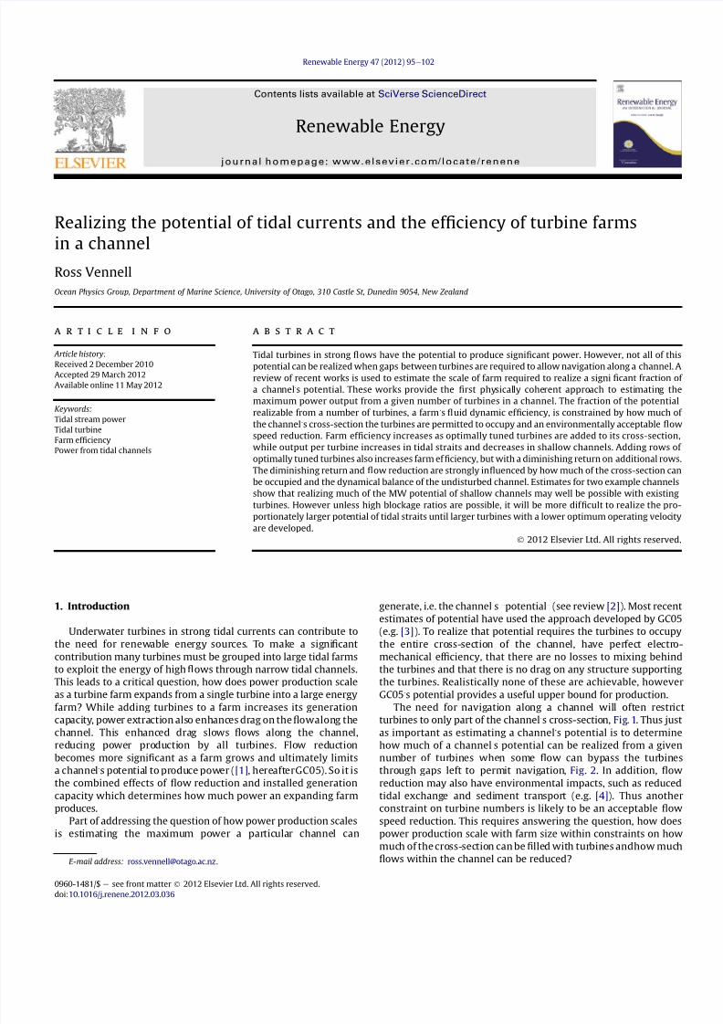
The underlying models are those of GC05 and GC07 adapted by
V10 and V11 In GC05rsquos model for a turbine farm in a short narrow
channel Fig 1 the farm is modelled as a drag on the 1047298ow The
model has oscillating tidal 1047298ow driven along the channel by a water
level difference between the ends of the channel This difference or
headloss is due to the differing tidal regimes in the two large water
bodies which are connected by the channel The water bodies are
assumed to be so large that any water 1047298owing through the channel
does not affect water levels within them Thus water levels at the
ends of the channel are unaffected by a power extraction within it
This is the simplest useful channel geometry One extension not
included here has a lagoon at one end of the channel and a large
ocean at the other [9] The 1047297nite reservoir of the lagoon means that
tides within it depend on the volume of water which1047298ows through
the channel As a result a lagoon can increase or decrease a tidal
channels potential depending on whether the amplitude of the
head between the ends of the channel is less than or greater than
the tidal amplitude in the ocean [10] In addition any large deep
ocean will likely have a shallow continental shelf between it and
the entrance to the channel Frictional dissipation and resonances
over the shelf may also in1047298uence the amplitudes of the tides at the
entrance to the channel driven by tides in the deep ocean [11]
The GC05 model is given in terms of volume transport here it is
presented in terms of velocity In short uniform cross-section
channels the cross-sectional average velocity does not vary signi1047297-
cantly along the channel [1213] Thus the tidal velocity everywhere
along a short channel with a rectangular cross-section depends only
ontimeand can beexpressedas u frac14 u0sinethut thorn fuTHORN where u0 is the
amplitude of the velocity and fu its phase GC05rsquos momentum
balance for a uniform cross-section channel can be written in the
form
vu
vt frac14
g z0
L sinethut THORN
C Dh thorn
C F
L
uu (1)
In Eq (1) the 1047297rst term represents the inertia of the 1047298ow the
second term the sinusoidal pressure gradient or head which forces
Fig 1 Schematic of a turbine farm in a narrow constricted channel connecting two
large water bodies Differing tidal regimes in the two large water bodies drive oscil-
lating tidal 1047298ow through the channel The example farm has 3 rows of turbines The
arrows around each turbine indicate the stronger 1047298ows passing around the turbines
and the weaker 1047298ows passing through the turbines
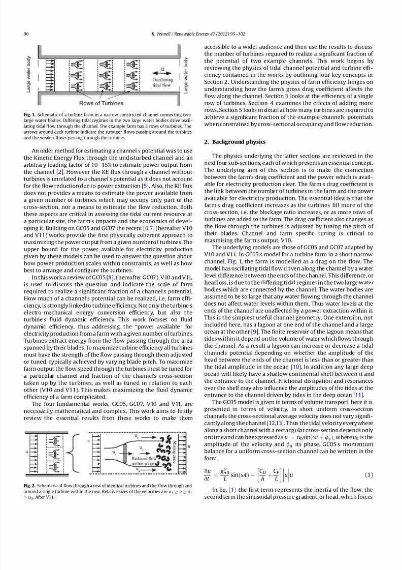
Fig 2 Schematic of 1047298ow through a row of identical turbines and the 1047298ow through and
around a single turbine within the row Relative sizes of the velocities are u4 u u1
u3 After V11
R Vennell Renewable Energy 47 (2012) 95e10296
8132019 Efficiency of Tidal Turbine Farms
httpslidepdfcomreaderfullefficiency-of-tidal-turbine-farms 38
8132019 Efficiency of Tidal Turbine Farms
httpslidepdfcomreaderfullefficiency-of-tidal-turbine-farms 48
adding turbines decreases the power lost to the turbines ie C F u30
decreases as the bene1047297t of growing the farm to increase C F is out-
weighed by the reduction in u0 due to the additional drag Between
these two extremes there is a maximum power which can be lost
by the 1047298ow to the turbines (GC05) as seen in the power lost curves
in Fig 3b) This maximum power lost to the turbines P maxlost is
a channelrsquos potential which is the upper bound for how much
power a channel can generate The optimal gross farm drag coef-
1047297cient C F peak required to realize the potential can be estimated
from the analytic solution to GC05rsquos model using (V10-A4) or (V11-
210) To realize a channelrsquos potential P maxlost turbines must occupy
the entire cross-section Were it possible around 25 turbines would
1047297ll the cross-section of the shallow channel and 2500 the cross-
section of the tidal strait Table 1 Many turbines sweep a circular
area thus cannot 1047297ll a rectangular channelrsquos cross-section unless
contained within a square shroud Thus the number of turbines
required to 1047297ll the cross-section N 0 may not always be of practical
use However N 0 is a useful as a reference value for the size of a farm
in later discussions on turbine numbers where they only 1047297ll part of the cross-section or are spread amongst rows
GC05 found a remarkably simple approximate expression for
estimating the potential of a channel based on the transport
amplitude through the undisturbed channel U 0UD frac14 Au0 and the
amplitude of the headloss z0 which is given by
P maxlost frac14 022r g z0U 0UD (4)
[10] gives a method to estimate both the potential and the 1047298ow
speed reduction which only requires the transport along the
undisturbed channel which is easily measured using a vessel
mounted ADCP eg [18]
23 Gaps between turbines allows 1047298ow to bypass turbines reducing the power available for power production GC07
When there are wide gaps between turbines within a row to
allow for navigation some 1047298ow bypasses the turbines altogether
and does not contribute to power production The mixing of the
retarded 1047298ow passing through the turbines with the faster 1047298ow
passing around the turbines also dissipates some of the 1047298owrsquos
energy as heat [19] and GC07 The 1047298ows near a row of turbines
are shown schematically in Fig 2 GC07 extended classic
Lanchester-Betz actuator disc theory for an isolated turbine [2021]
to a row of turbines in a narrow channel Fig 2 They found that the
rowrsquos drag coef 1047297cient C R depends only on the blockage ratio ε the
fraction of the channelrsquos cross-sectional area occupied by the
turbines and the ratio r 3 frac14 u3=u which quanti1047297
es the 1047298
ow
reduction in the wake behind the turbines ie they found C Rethε r 3THORN
Though the functional relationship is complex and given in equa-
tions (GC07-223 V10-26) and (GC07-29 V10-27) for the purpose
of this work it is only essential to understand that the drag coef 1047297-
cient of a row only varies due tothe changes in the blockage ratio or
changes in the 1047298ow reduction behind the turbines C Rethε r 3THORN
increases as either ε is increased or the 1047298ow in the wake r 3 is
decreased The fraction of the cross-section occupied by the
turbines ie the blockage ratio is simply
ε frac14 M AT
A
where M is the number of turbines in the row AT is area blocked by
the rotating by the blades of a single turbine
The average power lost by the 1047298ow is given by Eq (3) This is not
the same as the power available to the turbine for electricity
production due to mixing losses behind the turbines GC05 and
[19] Using their results the power available is the smaller work
done by the 1047298ow through the turbine Fu1 whose average is
P avail frac14 4
3pr Ar 1N RC Ru3
0 (5)
where r 1 frac14 u1=u is the ratio of the velocity though the turbines to
the velocity upstream of the row Comparing Eqs (3) and (5) shows
that dueto mixing lossesonly thefraction r 1 of the power lostby the
1047298ow tothe turbines is available forelectricity productionwhere0
r 1 1 The power available Eq (5) represents an upper bound for
electricity which could be produced from a farm in a channel
24 Turbines must be adjusted or tuned for a particular channel
and in relation to each other to maximize the power available V10
amp V11
Maximizing the powerlost by the1047298owdue tothe farm Eq (3) is
not the same as maximizing the power available for generation as
they differ bya factorof r 1 Eq (5) Fig 3b) demonstrates this where
the power lost curve peaks at C F peak while the lower power
available curvespeak at a smallerdrag coef 1047297cient C F opt indicated by
the dots To maximize the power available the 1047298ow through the
turbines must be adjusted or tuned to give the optimal farm drag
coef 1047297cient C F opt Typically tuning is done by adjusting the pitch of
the turbinersquos blades Here this tuning is done mathematically by
adjusting the value of the 1047298ow reduction r 3 which affects both C Rand r 1 GC07
GC07rsquos extension of Lanchester-Betz theory to turbines in
a channel assumed the 1047298
ow upstream of the row u in Fig 2 was
0 05 1 1504
06
08
1
F l o w r e d u c t i o n
U 0
U 0 u n d i s t u r b e d
CF C
Fpeak
a
0 05 1 150
02
04
06
08
1
P o w e r P
m a x
CF C
Fpeak
Decreasing tuning parameter r3 minusgt
b
Fig 3 Effects of increasing farmrsquos drag coef 1047297cient for two example channels in Table 1 Solid lines are for shallow channel and dashed lines for tidal strait Horizontal axis is the farm
drag coef 1047297cient relative to the drag coef 1047297cient required to realize a channelrsquos potential ie at the peak in the power lost curve a) Reduction in 1047298ow relative to 1047298ow in undisturbed
channel b) Thick lines are the power lost to the turbines and thin lines are the power available from 5 rows of turbines in the shallow channel and 40 rows in the tidal strait when
turbines occupy 20 of the channel rsquos cross-section Solid dots show peak in power available curves at optimal tuning ie the upper bound for how much power is available from
these turbines
R Vennell Renewable Energy 47 (2012) 95e10298
8132019 Efficiency of Tidal Turbine Farms
httpslidepdfcomreaderfullefficiency-of-tidal-turbine-farms 58
1047297xed and found an optimal value of r 3 frac14 1=3 (equivalent to
r 1 frac14 2=3) which maximised the power available the same optimal
values as those for an isolated Lanchester-Betz turbine They also
found that at most 23 of the power lost to the turbines was
available for power production which occurred if the turbines took
up the minimum possible fraction of the cross-section However in
a channel with 1047298ows driven by head loss between its ends the 1047298ow
upstream of the row u isnot 1047297xed but decreases as the farmrsquos gross
drag coef 1047297cient C F frac14 N RC Rethε r 3THORN increases Thus C F depends on
the tuning r 3 Consequently changing the tuning changes the
strength of the 1047298ow along the entire channel via its effect on the
gross drag coef 1047297cient V10 V10 went on to show that a conse-
quence of this is that turbines need r 3 to be tuned to valuesbetween
13 and 1 to maximize the power available Thus tuning a large tidal
farm is very different from tuning a single isolated device A farmrsquos
optimal tuning r opt3 depends on a channelrsquos geometry and
dynamical balance as well as the blockage ratio ε V10 found that
by optimally tuning turbines it is possible to exceed GC07rsquos
maximum of 23 of a channelrsquos potential which is available for
power production
V11 went on toshow that not only does a row of turbinesneed to
betuned fora particularchannelit must also betuned in thepresence
of other rows tomaximizethe poweravailableThe needto tunerowsldquoin-concertrdquo has implications for modellers who must include
idealizedturbines in theirhydrodynamicmodelsto assess the power
available from a proposed site V11 and for the operators of turbine
farms as turbines come in and out of service Tuning in-concert may
require many model runs or complex interdependent adjustment of
operating turbines to 1047297nd the optimal set of turbine tunings The
need to tune turbines in-concert arises because rows of turbines in
narrow channels interact with each other via the farmrsquos gross drag
coef 1047297cient C F even if they are separated widely enough for the
disturbed 1047298ow through onerow tofullymix before encountering the
next row as C F affects 1047298ow along the entire channel
3 Farm and turbine ef 1047297ciency for a single row
31 Farm 1047298uid dynamic ef 1047297ciency
A measure of a farmrsquos ef 1047297ciency is the fraction of GC05rsquos
potential which is available for power production V10 ie
FE frac14 P avail
P maxlost
(6)
FEis the farmrsquos 1047298uid dynamic power ef 1047297ciency and is maximised
at the optimal tuning r opt3 V11 This is the headline ef 1047297ciency which
is theupper bound forthe fractionof a channelrsquos estimated potential
that can be turned into electricity from a given number of turbines
Fig 4a) shows FE for the two example channels as optimally
tuned turbines are added to a single row The curves for both
examples converge on 1 as turbines take up most of the cross-
section making most of the channelrsquos potential available for
power production For the shallow channel farm ef 1047297ciency initially
grows rapidly as turbines are added with reduced gains at higher
numbers indicating a diminishing return on additional turbines In
contrast for the tidal strait FE increases more rapidly at the higher
occupancies indicating an increasing return on new turbines added
to the row V11 Though a farm in the shallow channel is more
ef 1047297cient than the tidal strait for a given fraction of the cross-section
occupied in absolute terms the tidal strait has a much larger power
available and requires many more turbines to make up this given
fraction The thin lines in Fig 4a) show the reduction in 1047298ow speeds
due to adding turbines to the row Flow in the shallow channel
decreases more rapidly as turbines are added consistent with its
higher farm ef 1047297ciency
Fig 4a) shows the 1047297rst of two extreme ways to almost realise
a channelrsquos potential ie approach 100 farm ef 1047297ciency is to have
the optimally tuned turbines 1047297ll the cross-section ie blockage
ratio ε1 Turbines are normally thought of as extracting energy
from the 1047298owrsquos Kinetic Energy by reducing 1047298ows through the
turbines However paradoxically an optimally tuned tidal farm canalmost realise a channelrsquos potential without reducing the 1047298ow
through the turbines relative to the 1047298ow upstream ie the optimal
r 3 and r 11 as ε1 V10 The resolution lies in understanding the
source of the farmrsquos energy For an isolated turbine generation is
a result of reducing 1047298ows through the turbine where for a Betz
turbine the optimal tuning is r 3 frac14 1=3 corresponding to r 1 frac14 2=3
As the cross-section is 1047297lled with turbines the farmrsquos energy source
changes gradually from the 1047298owrsquos KE to the potential energy of the
1047298ow as optimal tunings increase So that at high blockage ratios the
energy source becomes the drop in water level between the
upstream and downstream sides of the farm ie the source is the
headloss across the farm It is also worth emphasizing that mixing
losses behind the turbines approach zero at high blockage ratios
which must happen if farm ef 1047297ciency is to approach 100 At highblockage ratios turbine farms approach an extreme form of a hydro-
electric dam with low head and high volume 1047298ow For the two
examples the head loss is only around 01 10 m while the peak
volume 1047298ows are 27 000 1 700 000 m3s1 In contrast a large
river dam has high head and low 1047298ow ie a 100 m head and
500 m3s1
32 Power available per turbine
Fig 4b) gives the power available per turbine as the cross-
sections are 1047297lled with turbines A single isolated turbine ε0
in the shallow channel makes 099 MW available per turbine
0 02 04 06 08 10
02
04
06
08
1
Fraction of crossminussection occupied ε
P a v a i l P m a x
o r U 0
U 0 U Da
F a r m
E f f i
c i e n c
y
F l o w r e d u c t i o n
0 02 04 06 08 10
05
1
15
2
Fraction of crossminussection occupied ε
P o w e r p e r t u r b i n e M Wb
Fig 4 Effect of the fraction of cross-section occupied by the turbines or blockage ratio on ef 1047297ciencies and 1047298ow speeds for a single row of optimally tuned turbines in a uniform
cross-section channel Solid curves are for shallow channel and dashed lines for tidal strait examples a) Thick lines are farm ef 1047297ciency Eq (6) the fraction of GC05rsquos potential which
is available for power production and thin lines 1047298
ow relative to undisturbed channel b) Power available per turbine in MW
R Vennell Renewable Energy 47 (2012) 95e102 99
8132019 Efficiency of Tidal Turbine Farms
httpslidepdfcomreaderfullefficiency-of-tidal-turbine-farms 68
whereas only 034 MW is available in the tidal strait due to much
weaker 1047298ows However as the cross-section is 1047297lled the power
available per turbine for the shallow channel decreases while for
the tidal strait power per turbine increases So paradoxically at
higher occupancies the tidal strait delivers up to six times more per
turbine despite having much weaker 1047298ows than the shallow
channel The curves in Fig 4b) are the result of two competing
effects Firstly occupying more of the cross-section increases
a rowrsquos drag coef 1047297cient C R increases the power available Eq (5)
Secondly increasing a rows drag coef 1047297cient reduces the 1047298ow along
the channel U 0 which acts to decrease the power available in Eq
(5) The net effect differs for the two examples For the shallow
channel the more rapid reduction in 1047298ow speed as the cross-section
is 1047297lled Fig 4a) outweighs the enhanced drag coef 1047297cient leading
to reduction in the power per turbine from 099 MW to only
036 MW at high occupancy In contrast the more gradual 1047298ow
reduction in the tidal strait leads to an increasing power available
per turbine as the cross-section is 1047297lledfrom 034MW to23MW A
result is that above 35 occupancy the tidal strait delivers more per
turbine than the shallow channel despite the much weaker 1047298ows in
the strait
The differing performance of the turbines as the cross-section is
1047297lled is linked to their differing dynamical balances At higheroccupancies in the shallow channel the power lost to the turbines is
similar to that lost to background friction (this can be inferred from
(V10-A4) where C F peak is around twice the scaled background
bottom friction coef 1047297cient C D for near steady state channels ie
large l0 channels) This signi1047297cant energy loss to bottom friction
and turbine drag is associated with a more rapid decrease in 1047298ows
a diminishing return on new turbines and the decreasing power
available per turbine in Fig 4 In contrast in the tidal strait bottom
friction is almost unimportant and relatively little energy is lost to
bottom friction This gives the strait a proportionately higher
potential and an increasing return on additional turbines as they
becomemore ef 1047297cient when occupying more of the cross-section of
the ldquoductrdquo formed by the channel The energetics of channels with
turbine farms is discussed in detail in [17]
4 Ef 1047297ciency of multi-row farms
Adding capacity to a farm by adding rows of optimally tuned
turbines increases farm ef 1047297ciency as demonstrated in Fig 5a) For
the tidal strait 15 rows makes only 40 of it potential available so as
would be expected the associated 1047298ow reduction is modest In
contrast for the shallow channel 3 rows make 70 of its potential
available with a signi1047297cant associated 1047298ow reduction
Fig 5 illustrates a second extreme way to realize most of
a channelrsquos potential having a large number of rows However for
both channels there is a diminishing return on additional rows
Farm ef 1047297ciency peaks at a very large number of rows indicating an
optimal farm size However the diminishing return on new rows is
so harsh near this peak that farm size will be restricted to a much
smaller of number rows [17] V11 showed that for two similar
examples the best strategy for growing a farm of optimally tuned
turbines is the intuitive one Fill the 1047297rst row up to the maximum
permitted by navigational constraints and then add rows up to
a maximum that can be economically justi1047297ed in the light of the
diminishing returns inherent in Fig 5a)
5 Realizing the potential a trade off
The decision on turbine numbers is an economic trade off
between the income from the power made available by adding
turbines to a farm against their cost and any environmental
impacts Once the maximum permissible cross-sectional occu-
pancy has been achieved then the trade off is in the face of
a diminishing return on additional turbines Fig 5a) How this trade
off plays out depends strongly on the maximum fraction of the
channelrsquos cross-section which can be occupied in order to maintain
navigation along the channel It also strongly depends on the
dynamical balance of the undisturbed channel be it that of
a bottom friction dominated shallow channel or that of an inertia
dominated tidal strait Fig 5
This diminishing return is inherent in the upper row of plots in
Fig 6 where for both a low cross-sectional occupancy ε frac14 01 and
what may be an unrealistically high occupancy ε frac14 05 power
available increases more slowly as rows are added to an optimally
tuned farm While the ultimate choice on number of turbines
comes down to an economic and environmental cost bene1047297t
analysis which is beyond the scope of this work the plots however
do contain essential information to underpin this analysis For the
shallow channel at the high occupancy 1 row of 12 turbines makes
80 of its 9 MW potential available Fig 6a) In contrast the same
number of turbines spread across 5 rows at the lower occupancy
makes only 65 of the potential available for power productionFig 6c) shows that the power available per turbine for both occu-
pancies decreases as rows are added Fig 6e) illustrates that for
both occupancies a farm making 80 of the shallow channelrsquos
potential available will reduce 1047298ows by 30 If such a signi1047297cant
1047298ow reduction is not acceptable then at the lower occupancy
installing around 3 turbines reduces 1047298ows by only 10 while
making around 25 of its potential available
The curves for the tidal strait in Fig 6b) d) and f) are similar to
those of the shallow channel but the number of turbines involved
is much larger Almost 80 of the straitrsquos 6 GW potential can be
realized at the higher occupancy but this requires an astonishing
0 5 10 150
02
04
06
08
1
Number of Rows NR
a
Farm Efficiency
0 5 10 1504
06
08
1
Number of Rows NR
b
Flow reduction
Fig 5 Effect of adding rows to an optimally tuned farm where turbines occupy 20 of the channel rsquos cross-section ie a blockage ratio of ε frac14 02 Solid curves are for the shallow
channel and dashed lines for the tidal strait a) Farm ef 1047297
ciency Eq (6) b) Velocity relative to undisturbed velocity
R Vennell Renewable Energy 47 (2012) 95e102100
8132019 Efficiency of Tidal Turbine Farms
httpslidepdfcomreaderfullefficiency-of-tidal-turbine-farms 78
16000 turbines spread over 13 rows At the lower occupancy
a more affordable 5000 turbines would make 30 of the strait rsquos
potential available while reducing 1047298ows by 7
6 Discussion
The principle aim of this paper was to show how many turbines
are required to realize a given fraction of a channel rsquos potential in
order to improve understanding of how power production scales
with farm size The models in V10 and V11 which build on those of
GC05 and GC07 provide the 1047297rst physically coherent way of con-
necting the number of turbines in a farm with the maximum power
available for electricity production The models do not require the
use of arbitrary loading or safety factors applied to account for
unknown effects The models are however simple They use an
extended form of classic turbine theory and they only apply to the
cross-sectional average velocities thusdo not account for the effects
of any variation of 1047298ow across the channel or with depth They also
do not allow for any effect of the turbulence shed by a row on the
ef 1047297
ciency of downstream rows They do not allow for minimum
turbine operating 1047298ows or for loss due to their electro-mechanical
ef 1047297ciency or transmission and conversion losses Thus there is
muchworktobedonetore1047297ne and extend the modelsHowever the
models do illuminate signi1047297cant aspects of developing large tidal
turbine farms Most of these are a result of power extraction
reducing the 1047298ows along the entire narrow channel via the farmrsquos
gross dragcoef 1047297cient C F They include thenecessity totune turbines
for the particular channel and in relation to each other which will
result in signi1047297cant computational cost to those modelling turbine
farms and will require on going optimization of turbine tuning in
large operational farms as turbines come in and out of service They
also include how farms have increasing or diminishing returns on
turbines added to thecross-section dependingon the importance of
bottom friction and how there is always a diminishing return on
additional rows aspects which are fundamental to understanding
the economics of farm development
The turbine numbers given by the simple models should be
viewed as estimates of the magnitude of the numbers required
rather than precise estimates These magnitudes are useful in
understanding how realistic it is to realize a signi1047297
cant fraction of
0 10 20 30 400
02
04
06
08
1
1
3
5
101
3
P o w e r P
m a x
Number of Turbines
aShallow Channel
0 5 10 150
02
04
06
08
1
1
5
10
20
50
1
5
10
P o w e r P
m a x
Thousands of Turbines
bTidal Strait
0 10 20 30 400
02
04
06
08
1
12
P o w
e r P e r T u r b i n e M W
Number of Turbines
c
0 5 100
02
04
06
08
1
12
P o w
e r P e r T u r b i n e M W
Thousands of Turbines
d
06 07 08 09 10
02
04
06
08
1
5
10
15
2515
25
P o w e r P
m a x
Flow Reduction
e
06 07 08 09 10
02
04
06
08
1
10002000
5000
10000
15000
2000
5000
10000
15000
P o w e r P
m a x
Flow Reduction
f
Fig 6 Effect of the number of optimally tuned turbines on power available and 1047298ow reduction for the two example channels based on a 400 m 2 blade area Solid curves are for
ε frac14 01 and dashed lines for ε frac14 05 a) and b) Farm ef 1047297ciency versus number of turbines labelled dots give number of rows in the farm c) and d) Power available per turbine in
MW e) and f) Farm ef 1047297ciency verses 1047298ow reduction Labelled dots give the number of turbines in farm
R Vennell Renewable Energy 47 (2012) 95e102 101
8132019 Efficiency of Tidal Turbine Farms
httpslidepdfcomreaderfullefficiency-of-tidal-turbine-farms 88
a channelrsquos potential For the shallow channel around eight 400 m2
turbines corresponding to three rows with ε frac14 01 makes half of
its potential available and 13 corresponding to one row with
ε frac14 05 makes 80 available Table 1 The given values for the
power available per turbine are also useful in understanding
economic feasibility For blockage ratios of ε frac14 01 and 05 each
turbine makes around 06 MW available The detailed economics
and environmental costs are beyond the scope of this work
however making an average of 06 MWavailable over the tidal cycle
when existing turbines are producing around 1 MW at steady1047298ows
around2 m s1 maybe a reasonable return Thus it appears possible
to make a signi1047297cant fraction of the shallow channelrsquos potential
available using 5e10 turbines with a blade area similar to that of
the largest currently operating tidal turbine spread amongst 1e3
rows which occupy less than 50 of the cross-section
In contrast to make 50 of the tidal straitrsquos 6 GW potential
available takes 10000 turbines at 10 blockage This high number
is a result of the weaker 1047298ows in the tidal strait which yield only
027 MW per turbine However unlike the tidal shallow channel
the output per turbine rises as more of the strait rsquos cross-section is
occupied So that at 50 blockage only 5000 turbines are required
to make 50 of its potentialavailable at a much higher 061MW per
turbine similar to that for the shallow channel Tidal straits haveboth a much larger potential in absolute terms and in proportion to
their size due to relatively low energy losses to bottom friction
This is seen in their having six times the potential per turbinewhen
turbines 1047297ll the cross-section in a single row Table 1 However tidal
straits typically have weaker cross-sectionally averaged 1047298ows than
shallow tidal channels Thus at low blockage ratios a very large
number of rows are required to make a signi1047297cant fraction avail-
able If higher blockage ratios are permitted then the enhanced
ef 1047297ciency of turbines in tidal straits seen in Fig 4 boosts the output
per turbine and reduces the total number of turbines required [17]
uses the channelrsquos energy balance to explain why and when tidal
straits have an increasing return on turbines added to the cross-
section and why shallow channels have a diminishing return
7 Conclusions
Critical questions in developing a farm are what fraction of
a channelrsquos potential is available for power production from a given
number of turbines as a farm scales up from a single turbine into
a large farm The V10 thorn V11 works provide the 1047297rst physically
coherent way to connect the number of turbines in a farm to both
the maximum power available for electricity production and to the
degree of 1047298ow reduction which is a consequence of power
extraction Though simple they illuminate several important
aspects of developing large farms which have implications for both
the economics and environmental impact of farms Such as the
necessity of tuning turbines in large farms for the particular
channel how much of the cross-section they occupy and the
number of rows as well as how to best arrange and con1047297gure the
turbines For example to maximize farm ef 1047297ciency the 1047297rst row
turbines should be 1047297lled up to the maximum permitted by navi-
gational constraints before adding new rows Also while farm
ef 1047297ciency always increases as optimally tuned turbines are added
once the cross-sectional occupancy limit is attained the power
available per turbine decreases as rows are added Thus increasing
power production by increasing the farmrsquos installed capacity faces
a diminishing return on additional rows This development strategy
may alter when more realistic models are developed which allow
for variation of 1047298ow across the channel and with depth However
the decision on turbine numbers will remain an economic trade off
between the power produced and installation maintenance and
environmental costs How this trade off plays out depends strongly
on the maximum fraction of the channelrsquos cross-section which can
be occupied and the dynamical balance of the undisturbed channel
The examples demonstrate that it may be possible with existing
technology to realize much of the MW potential of shallow tidal
channels The GW potential of tidal straits is both larger in absolute
terms and also proportionately larger than that of shallow chan-
nels due to relatively low energy losses to bottom friction At low
cross-sectional occupancies the typically lower 1047298ows of the strait
result in both a low return per turbine and a very large number of
turbines being required to realize a signi1047297cant fraction of their
proportionately higher potential Thus unless a large fraction of the
straitrsquos cross-section can be occupied to take advantage of a higher
output per turbine it will be dif 1047297cult to realize a substantial frac-
tion of the GW potential of tidal straits until larger turbines are
developed which are able operate economically in low 1047298ows
References
[1] Garrett C Cummins P The power potential of tidal currents in channels
Proceedings of the Royal Society A 20054612563e
72[2] Blunden LS Bahaj AS Tidal energy resource assessment for tidal stream
generators Proceedings of the Institution of Mechanical Engineers Part A Journal of Power and Energy 2007221(10)137e46 doi10124309576509JPE332
[3] Blanch1047297eld J Garrett C Rowe A Wild P Tidal stream power resourceassessment for Masset Sound Haida Gwaii Proceedings of the Institution of Mechanical Engineers Part A Journal of Power and Energy 2008222(5)485e92
[4] Neill SP Litt EJ Couch SJ Davies AG The impact of tidal stream turbines onlarge-scale sediment dynamics Renewable Energy 200934(12)2803e12doi101016jrenene200906015
[5] Garrett C Cummins P Limits to tidal current power Renewable Energy 2008332485e90
[6] Garrett C Cummins P Tuning turbines in a tidal channel Journal of FluidMechanics 2010663253e67 doi101017S0022112010003502
[7] Vennell R Tuning tidal turbines in concert to maximise farm ef 1047297ciency Journal of Fluid Mechanics 2011671587e604
[8] Garrett C Cummins P The ef 1047297
ciency of a turbine in a tidal channel Journal of Fluid Mechanics 2007588243e51[9] Blanch1047297eld J Garrett C Wild P Rowe A The extractable power from a channel
linking a bay to the open ocean Proceedings of the Institution of MechanicalEngineers Part A Journal of Power and Energy 2008222(3)289e97
[10] Vennell R Estimating the power potential of tidal currents and the impact of power extraction on 1047298ow speeds Renewable Energy 2011363558e65 doi101016jrenene201105011
[11] Arbic B Garrett C A coupled oscillator model of shelf and ocean tidesContinental Shelf Research 201030(6)564e74
[12] Vennell R Oscillating barotropic currents along short channels Journal of Physical Oceanography 199828(8)1561e9
[13] Vennell R Observations of the phase of tidal currents along a strait Journal of Physical Oceanography 199828(8)1570e7
[14] Byden IG Grinsted T Melville GT Assessing the potential of a simple tidalchannel to deliver useful energy Journal of Applied Ocean Research 200426198e204 doi101016japor200504001
[15] Vennell R ADCP measurements of tidal phase and amplitude in Cook StraitNew Zealand Continental Shelf Research 199414353e64
[16] Douglas C Harrison G Chick J Life cycle assessment of the Seagen marinecurrent turbine Proceedings of the Institution of Mechanical Engineers Part M
Journal of Engineering for the Maritime Environment 2008222(1)1e12 doi10124314750902JEME94
[17] Vennell R The energetics of large tidal turbine arrays Renewable Energyin press
[18] Vennell R ADCP measurements of momentum balance and dynamic topog-raphy in a constricted tidal channel Journal of Physical Oceanography 200636(2)177e88
[19] Corten G Heat generation by a wind turbine Vol In 14th IEA symposium onthe aerodynamics of wind turbines 2000 p 7 ECN report ECN-RX-01-001
[20] Lanchester FW A contribution to the theory of propulsion and the screwpropeller Transactions of the Institution of Naval Architects 1915LVII98e116
[21] Betz A Das Maximum der theoretisch moumlglichen Ausnutzung des Windesdurch Windmotoren Gesamte Turbinenwesen 192017307e9
R Vennell Renewable Energy 47 (2012) 95e102102
8132019 Efficiency of Tidal Turbine Farms
httpslidepdfcomreaderfullefficiency-of-tidal-turbine-farms 28
An older method for estimating a channelrsquos potential was to use
the Kinetic Energy Flux through the undisturbed channel and an
arbitrary loading factor of 10e15 to estimate power output from
the channel [2] However the KE 1047298ux through a channel without
turbines is unrelated to a channelrsquos potential as it does not account
for the 1047298ow reduction due to power extraction [5] Also the KE 1047298ux
does not provides a means to estimate the power available from
a given number of turbines which may occupy only part of thecross-section nor a means to estimate the 1047298ow reduction Both
these aspects are critical in assessing the tidal current resource at
a particular site the farmrsquos impacts and the economics of devel-
oping it Building on GC05 and GC07 the recent [67] (hereafter V10
and V11) works provide the 1047297rst physically coherent approach to
maximizing the poweroutput from a given numberof turbinesThe
upper bound for the power available for electricity production
given by these models can be used to answer the question about
how power production scales within constraints as well as how
best to arrange and con1047297gure the turbines
In this work a review of GC05 [8] (hereafter GC07) V10 and V11
is used to discuss the question and indicate the scale of farm
required to realize a signi1047297cant fraction of a channelrsquos potential
How much of a channelrsquos potential can be realized ie farm ef 1047297-
ciency is strongly linkedto turbine ef 1047297ciency Not only the turbinersquos
electro-mechanical energy conversion ef 1047297ciency but also the
turbinersquos 1047298uid dynamic ef 1047297ciency This work focuses on 1047298uid
dynamic ef 1047297ciency thus addressing the ldquopower availablerdquo for
electricity production from a farm with a given number of turbines
Turbines extract energy from the 1047298ow passing through the area
spanned by their blades To maximize turbine ef 1047297ciency all turbines
must have the strength of the 1047298ow passing through them adjusted
or tuned typically achieved by varying blade pitch To maximize
farm output the 1047298ow speed through the turbines must be tuned for
a particular channel and fraction of the channelrsquos cross-section
taken up by the turbines as well as tuned in relation to each
other (V10 and V11) This makes maximizing the 1047298uid dynamic
ef 1047297
ciency of a farm complicatedThe four fundamental works GC05 GC07 V10 and V11 are
necessarily mathematical and complex This work aims to 1047297rstly
review the essential results from these works to make them
accessible to a wider audience and then use the results to discuss
the number of turbines required to realize a signi1047297cant fraction of
the potential of two example channels This work begins by
reviewing the physics of tidal channel potential and turbine ef 1047297-
ciency contained in the works by outlining four key concepts in
Section 2 Understanding the physics of farm ef 1047297ciency hinges on
understanding how the farmrsquos gross drag coef 1047297cient affects the
1047298ow along the channel Section 3 looks at the ef 1047297ciency of a single
row of turbines Section 4 examines the effects of adding more
rows Section 5 looks in detail at how many turbines are required to
achieve a signi1047297cant fraction of the example channelsrsquo potentials
when constrained by cross-sectional occupancy and 1047298ow reduction
2 Background physics
The physics underlying the latter sections are reviewed in the
next four sub-sections each of which presents an essential concept
The underlying aim of this section is to make the connection
between the farmrsquos drag coef 1047297cient and the power which is avail-
able for electricity production clear The farmrsquos drag coef 1047297cient is
the link between the number of turbines in the farm and the power
available for electricity production The essential idea is that thefarmrsquos drag coef 1047297cient increases as the turbines 1047297ll more of the
cross-section ie the blockage ratio increases or as more rows of
turbines are added to the farm The drag coef 1047297cient also changes as
the 1047298ow through the turbines is adjusted by tuning the pitch of
their blades Channel and farm speci1047297c tuning is critical to
maxmising the farmrsquos output V10
The underlying models are those of GC05 and GC07 adapted by
V10 and V11 In GC05rsquos model for a turbine farm in a short narrow
channel Fig 1 the farm is modelled as a drag on the 1047298ow The
model has oscillating tidal 1047298ow driven along the channel by a water
level difference between the ends of the channel This difference or
headloss is due to the differing tidal regimes in the two large water
bodies which are connected by the channel The water bodies are
assumed to be so large that any water 1047298owing through the channel
does not affect water levels within them Thus water levels at the
ends of the channel are unaffected by a power extraction within it
This is the simplest useful channel geometry One extension not
included here has a lagoon at one end of the channel and a large
ocean at the other [9] The 1047297nite reservoir of the lagoon means that
tides within it depend on the volume of water which1047298ows through
the channel As a result a lagoon can increase or decrease a tidal
channels potential depending on whether the amplitude of the
head between the ends of the channel is less than or greater than
the tidal amplitude in the ocean [10] In addition any large deep
ocean will likely have a shallow continental shelf between it and
the entrance to the channel Frictional dissipation and resonances
over the shelf may also in1047298uence the amplitudes of the tides at the
entrance to the channel driven by tides in the deep ocean [11]
The GC05 model is given in terms of volume transport here it is
presented in terms of velocity In short uniform cross-section
channels the cross-sectional average velocity does not vary signi1047297-
cantly along the channel [1213] Thus the tidal velocity everywhere
along a short channel with a rectangular cross-section depends only
ontimeand can beexpressedas u frac14 u0sinethut thorn fuTHORN where u0 is the
amplitude of the velocity and fu its phase GC05rsquos momentum
balance for a uniform cross-section channel can be written in the
form
vu
vt frac14
g z0
L sinethut THORN
C Dh thorn
C F
L
uu (1)
In Eq (1) the 1047297rst term represents the inertia of the 1047298ow the
second term the sinusoidal pressure gradient or head which forces
Fig 1 Schematic of a turbine farm in a narrow constricted channel connecting two
large water bodies Differing tidal regimes in the two large water bodies drive oscil-
lating tidal 1047298ow through the channel The example farm has 3 rows of turbines The
arrows around each turbine indicate the stronger 1047298ows passing around the turbines
and the weaker 1047298ows passing through the turbines
Fig 2 Schematic of 1047298ow through a row of identical turbines and the 1047298ow through and
around a single turbine within the row Relative sizes of the velocities are u4 u u1
u3 After V11
R Vennell Renewable Energy 47 (2012) 95e10296
8132019 Efficiency of Tidal Turbine Farms
httpslidepdfcomreaderfullefficiency-of-tidal-turbine-farms 38
8132019 Efficiency of Tidal Turbine Farms
httpslidepdfcomreaderfullefficiency-of-tidal-turbine-farms 48
adding turbines decreases the power lost to the turbines ie C F u30
decreases as the bene1047297t of growing the farm to increase C F is out-
weighed by the reduction in u0 due to the additional drag Between
these two extremes there is a maximum power which can be lost
by the 1047298ow to the turbines (GC05) as seen in the power lost curves
in Fig 3b) This maximum power lost to the turbines P maxlost is
a channelrsquos potential which is the upper bound for how much
power a channel can generate The optimal gross farm drag coef-
1047297cient C F peak required to realize the potential can be estimated
from the analytic solution to GC05rsquos model using (V10-A4) or (V11-
210) To realize a channelrsquos potential P maxlost turbines must occupy
the entire cross-section Were it possible around 25 turbines would
1047297ll the cross-section of the shallow channel and 2500 the cross-
section of the tidal strait Table 1 Many turbines sweep a circular
area thus cannot 1047297ll a rectangular channelrsquos cross-section unless
contained within a square shroud Thus the number of turbines
required to 1047297ll the cross-section N 0 may not always be of practical
use However N 0 is a useful as a reference value for the size of a farm
in later discussions on turbine numbers where they only 1047297ll part of the cross-section or are spread amongst rows
GC05 found a remarkably simple approximate expression for
estimating the potential of a channel based on the transport
amplitude through the undisturbed channel U 0UD frac14 Au0 and the
amplitude of the headloss z0 which is given by
P maxlost frac14 022r g z0U 0UD (4)
[10] gives a method to estimate both the potential and the 1047298ow
speed reduction which only requires the transport along the
undisturbed channel which is easily measured using a vessel
mounted ADCP eg [18]
23 Gaps between turbines allows 1047298ow to bypass turbines reducing the power available for power production GC07
When there are wide gaps between turbines within a row to
allow for navigation some 1047298ow bypasses the turbines altogether
and does not contribute to power production The mixing of the
retarded 1047298ow passing through the turbines with the faster 1047298ow
passing around the turbines also dissipates some of the 1047298owrsquos
energy as heat [19] and GC07 The 1047298ows near a row of turbines
are shown schematically in Fig 2 GC07 extended classic
Lanchester-Betz actuator disc theory for an isolated turbine [2021]
to a row of turbines in a narrow channel Fig 2 They found that the
rowrsquos drag coef 1047297cient C R depends only on the blockage ratio ε the
fraction of the channelrsquos cross-sectional area occupied by the
turbines and the ratio r 3 frac14 u3=u which quanti1047297
es the 1047298
ow
reduction in the wake behind the turbines ie they found C Rethε r 3THORN
Though the functional relationship is complex and given in equa-
tions (GC07-223 V10-26) and (GC07-29 V10-27) for the purpose
of this work it is only essential to understand that the drag coef 1047297-
cient of a row only varies due tothe changes in the blockage ratio or
changes in the 1047298ow reduction behind the turbines C Rethε r 3THORN
increases as either ε is increased or the 1047298ow in the wake r 3 is
decreased The fraction of the cross-section occupied by the
turbines ie the blockage ratio is simply
ε frac14 M AT
A
where M is the number of turbines in the row AT is area blocked by
the rotating by the blades of a single turbine
The average power lost by the 1047298ow is given by Eq (3) This is not
the same as the power available to the turbine for electricity
production due to mixing losses behind the turbines GC05 and
[19] Using their results the power available is the smaller work
done by the 1047298ow through the turbine Fu1 whose average is
P avail frac14 4
3pr Ar 1N RC Ru3
0 (5)
where r 1 frac14 u1=u is the ratio of the velocity though the turbines to
the velocity upstream of the row Comparing Eqs (3) and (5) shows
that dueto mixing lossesonly thefraction r 1 of the power lostby the
1047298ow tothe turbines is available forelectricity productionwhere0
r 1 1 The power available Eq (5) represents an upper bound for
electricity which could be produced from a farm in a channel
24 Turbines must be adjusted or tuned for a particular channel
and in relation to each other to maximize the power available V10
amp V11
Maximizing the powerlost by the1047298owdue tothe farm Eq (3) is
not the same as maximizing the power available for generation as
they differ bya factorof r 1 Eq (5) Fig 3b) demonstrates this where
the power lost curve peaks at C F peak while the lower power
available curvespeak at a smallerdrag coef 1047297cient C F opt indicated by
the dots To maximize the power available the 1047298ow through the
turbines must be adjusted or tuned to give the optimal farm drag
coef 1047297cient C F opt Typically tuning is done by adjusting the pitch of
the turbinersquos blades Here this tuning is done mathematically by
adjusting the value of the 1047298ow reduction r 3 which affects both C Rand r 1 GC07
GC07rsquos extension of Lanchester-Betz theory to turbines in
a channel assumed the 1047298
ow upstream of the row u in Fig 2 was
0 05 1 1504
06
08
1
F l o w r e d u c t i o n
U 0
U 0 u n d i s t u r b e d
CF C
Fpeak
a
0 05 1 150
02
04
06
08
1
P o w e r P
m a x
CF C
Fpeak
Decreasing tuning parameter r3 minusgt
b
Fig 3 Effects of increasing farmrsquos drag coef 1047297cient for two example channels in Table 1 Solid lines are for shallow channel and dashed lines for tidal strait Horizontal axis is the farm
drag coef 1047297cient relative to the drag coef 1047297cient required to realize a channelrsquos potential ie at the peak in the power lost curve a) Reduction in 1047298ow relative to 1047298ow in undisturbed
channel b) Thick lines are the power lost to the turbines and thin lines are the power available from 5 rows of turbines in the shallow channel and 40 rows in the tidal strait when
turbines occupy 20 of the channel rsquos cross-section Solid dots show peak in power available curves at optimal tuning ie the upper bound for how much power is available from
these turbines
R Vennell Renewable Energy 47 (2012) 95e10298
8132019 Efficiency of Tidal Turbine Farms
httpslidepdfcomreaderfullefficiency-of-tidal-turbine-farms 58
1047297xed and found an optimal value of r 3 frac14 1=3 (equivalent to
r 1 frac14 2=3) which maximised the power available the same optimal
values as those for an isolated Lanchester-Betz turbine They also
found that at most 23 of the power lost to the turbines was
available for power production which occurred if the turbines took
up the minimum possible fraction of the cross-section However in
a channel with 1047298ows driven by head loss between its ends the 1047298ow
upstream of the row u isnot 1047297xed but decreases as the farmrsquos gross
drag coef 1047297cient C F frac14 N RC Rethε r 3THORN increases Thus C F depends on
the tuning r 3 Consequently changing the tuning changes the
strength of the 1047298ow along the entire channel via its effect on the
gross drag coef 1047297cient V10 V10 went on to show that a conse-
quence of this is that turbines need r 3 to be tuned to valuesbetween
13 and 1 to maximize the power available Thus tuning a large tidal
farm is very different from tuning a single isolated device A farmrsquos
optimal tuning r opt3 depends on a channelrsquos geometry and
dynamical balance as well as the blockage ratio ε V10 found that
by optimally tuning turbines it is possible to exceed GC07rsquos
maximum of 23 of a channelrsquos potential which is available for
power production
V11 went on toshow that not only does a row of turbinesneed to
betuned fora particularchannelit must also betuned in thepresence
of other rows tomaximizethe poweravailableThe needto tunerowsldquoin-concertrdquo has implications for modellers who must include
idealizedturbines in theirhydrodynamicmodelsto assess the power
available from a proposed site V11 and for the operators of turbine
farms as turbines come in and out of service Tuning in-concert may
require many model runs or complex interdependent adjustment of
operating turbines to 1047297nd the optimal set of turbine tunings The
need to tune turbines in-concert arises because rows of turbines in
narrow channels interact with each other via the farmrsquos gross drag
coef 1047297cient C F even if they are separated widely enough for the
disturbed 1047298ow through onerow tofullymix before encountering the
next row as C F affects 1047298ow along the entire channel
3 Farm and turbine ef 1047297ciency for a single row
31 Farm 1047298uid dynamic ef 1047297ciency
A measure of a farmrsquos ef 1047297ciency is the fraction of GC05rsquos
potential which is available for power production V10 ie
FE frac14 P avail
P maxlost
(6)
FEis the farmrsquos 1047298uid dynamic power ef 1047297ciency and is maximised
at the optimal tuning r opt3 V11 This is the headline ef 1047297ciency which
is theupper bound forthe fractionof a channelrsquos estimated potential
that can be turned into electricity from a given number of turbines
Fig 4a) shows FE for the two example channels as optimally
tuned turbines are added to a single row The curves for both
examples converge on 1 as turbines take up most of the cross-
section making most of the channelrsquos potential available for
power production For the shallow channel farm ef 1047297ciency initially
grows rapidly as turbines are added with reduced gains at higher
numbers indicating a diminishing return on additional turbines In
contrast for the tidal strait FE increases more rapidly at the higher
occupancies indicating an increasing return on new turbines added
to the row V11 Though a farm in the shallow channel is more
ef 1047297cient than the tidal strait for a given fraction of the cross-section
occupied in absolute terms the tidal strait has a much larger power
available and requires many more turbines to make up this given
fraction The thin lines in Fig 4a) show the reduction in 1047298ow speeds
due to adding turbines to the row Flow in the shallow channel
decreases more rapidly as turbines are added consistent with its
higher farm ef 1047297ciency
Fig 4a) shows the 1047297rst of two extreme ways to almost realise
a channelrsquos potential ie approach 100 farm ef 1047297ciency is to have
the optimally tuned turbines 1047297ll the cross-section ie blockage
ratio ε1 Turbines are normally thought of as extracting energy
from the 1047298owrsquos Kinetic Energy by reducing 1047298ows through the
turbines However paradoxically an optimally tuned tidal farm canalmost realise a channelrsquos potential without reducing the 1047298ow
through the turbines relative to the 1047298ow upstream ie the optimal
r 3 and r 11 as ε1 V10 The resolution lies in understanding the
source of the farmrsquos energy For an isolated turbine generation is
a result of reducing 1047298ows through the turbine where for a Betz
turbine the optimal tuning is r 3 frac14 1=3 corresponding to r 1 frac14 2=3
As the cross-section is 1047297lled with turbines the farmrsquos energy source
changes gradually from the 1047298owrsquos KE to the potential energy of the
1047298ow as optimal tunings increase So that at high blockage ratios the
energy source becomes the drop in water level between the
upstream and downstream sides of the farm ie the source is the
headloss across the farm It is also worth emphasizing that mixing
losses behind the turbines approach zero at high blockage ratios
which must happen if farm ef 1047297ciency is to approach 100 At highblockage ratios turbine farms approach an extreme form of a hydro-
electric dam with low head and high volume 1047298ow For the two
examples the head loss is only around 01 10 m while the peak
volume 1047298ows are 27 000 1 700 000 m3s1 In contrast a large
river dam has high head and low 1047298ow ie a 100 m head and
500 m3s1
32 Power available per turbine
Fig 4b) gives the power available per turbine as the cross-
sections are 1047297lled with turbines A single isolated turbine ε0
in the shallow channel makes 099 MW available per turbine
0 02 04 06 08 10
02
04
06
08
1
Fraction of crossminussection occupied ε
P a v a i l P m a x
o r U 0
U 0 U Da
F a r m
E f f i
c i e n c
y
F l o w r e d u c t i o n
0 02 04 06 08 10
05
1
15
2
Fraction of crossminussection occupied ε
P o w e r p e r t u r b i n e M Wb
Fig 4 Effect of the fraction of cross-section occupied by the turbines or blockage ratio on ef 1047297ciencies and 1047298ow speeds for a single row of optimally tuned turbines in a uniform
cross-section channel Solid curves are for shallow channel and dashed lines for tidal strait examples a) Thick lines are farm ef 1047297ciency Eq (6) the fraction of GC05rsquos potential which
is available for power production and thin lines 1047298
ow relative to undisturbed channel b) Power available per turbine in MW
R Vennell Renewable Energy 47 (2012) 95e102 99
8132019 Efficiency of Tidal Turbine Farms
httpslidepdfcomreaderfullefficiency-of-tidal-turbine-farms 68
whereas only 034 MW is available in the tidal strait due to much
weaker 1047298ows However as the cross-section is 1047297lled the power
available per turbine for the shallow channel decreases while for
the tidal strait power per turbine increases So paradoxically at
higher occupancies the tidal strait delivers up to six times more per
turbine despite having much weaker 1047298ows than the shallow
channel The curves in Fig 4b) are the result of two competing
effects Firstly occupying more of the cross-section increases
a rowrsquos drag coef 1047297cient C R increases the power available Eq (5)
Secondly increasing a rows drag coef 1047297cient reduces the 1047298ow along
the channel U 0 which acts to decrease the power available in Eq
(5) The net effect differs for the two examples For the shallow
channel the more rapid reduction in 1047298ow speed as the cross-section
is 1047297lled Fig 4a) outweighs the enhanced drag coef 1047297cient leading
to reduction in the power per turbine from 099 MW to only
036 MW at high occupancy In contrast the more gradual 1047298ow
reduction in the tidal strait leads to an increasing power available
per turbine as the cross-section is 1047297lledfrom 034MW to23MW A
result is that above 35 occupancy the tidal strait delivers more per
turbine than the shallow channel despite the much weaker 1047298ows in
the strait
The differing performance of the turbines as the cross-section is
1047297lled is linked to their differing dynamical balances At higheroccupancies in the shallow channel the power lost to the turbines is
similar to that lost to background friction (this can be inferred from
(V10-A4) where C F peak is around twice the scaled background
bottom friction coef 1047297cient C D for near steady state channels ie
large l0 channels) This signi1047297cant energy loss to bottom friction
and turbine drag is associated with a more rapid decrease in 1047298ows
a diminishing return on new turbines and the decreasing power
available per turbine in Fig 4 In contrast in the tidal strait bottom
friction is almost unimportant and relatively little energy is lost to
bottom friction This gives the strait a proportionately higher
potential and an increasing return on additional turbines as they
becomemore ef 1047297cient when occupying more of the cross-section of
the ldquoductrdquo formed by the channel The energetics of channels with
turbine farms is discussed in detail in [17]
4 Ef 1047297ciency of multi-row farms
Adding capacity to a farm by adding rows of optimally tuned
turbines increases farm ef 1047297ciency as demonstrated in Fig 5a) For
the tidal strait 15 rows makes only 40 of it potential available so as
would be expected the associated 1047298ow reduction is modest In
contrast for the shallow channel 3 rows make 70 of its potential
available with a signi1047297cant associated 1047298ow reduction
Fig 5 illustrates a second extreme way to realize most of
a channelrsquos potential having a large number of rows However for
both channels there is a diminishing return on additional rows
Farm ef 1047297ciency peaks at a very large number of rows indicating an
optimal farm size However the diminishing return on new rows is
so harsh near this peak that farm size will be restricted to a much
smaller of number rows [17] V11 showed that for two similar
examples the best strategy for growing a farm of optimally tuned
turbines is the intuitive one Fill the 1047297rst row up to the maximum
permitted by navigational constraints and then add rows up to
a maximum that can be economically justi1047297ed in the light of the
diminishing returns inherent in Fig 5a)
5 Realizing the potential a trade off
The decision on turbine numbers is an economic trade off
between the income from the power made available by adding
turbines to a farm against their cost and any environmental
impacts Once the maximum permissible cross-sectional occu-
pancy has been achieved then the trade off is in the face of
a diminishing return on additional turbines Fig 5a) How this trade
off plays out depends strongly on the maximum fraction of the
channelrsquos cross-section which can be occupied in order to maintain
navigation along the channel It also strongly depends on the
dynamical balance of the undisturbed channel be it that of
a bottom friction dominated shallow channel or that of an inertia
dominated tidal strait Fig 5
This diminishing return is inherent in the upper row of plots in
Fig 6 where for both a low cross-sectional occupancy ε frac14 01 and
what may be an unrealistically high occupancy ε frac14 05 power
available increases more slowly as rows are added to an optimally
tuned farm While the ultimate choice on number of turbines
comes down to an economic and environmental cost bene1047297t
analysis which is beyond the scope of this work the plots however
do contain essential information to underpin this analysis For the
shallow channel at the high occupancy 1 row of 12 turbines makes
80 of its 9 MW potential available Fig 6a) In contrast the same
number of turbines spread across 5 rows at the lower occupancy
makes only 65 of the potential available for power productionFig 6c) shows that the power available per turbine for both occu-
pancies decreases as rows are added Fig 6e) illustrates that for
both occupancies a farm making 80 of the shallow channelrsquos
potential available will reduce 1047298ows by 30 If such a signi1047297cant
1047298ow reduction is not acceptable then at the lower occupancy
installing around 3 turbines reduces 1047298ows by only 10 while
making around 25 of its potential available
The curves for the tidal strait in Fig 6b) d) and f) are similar to
those of the shallow channel but the number of turbines involved
is much larger Almost 80 of the straitrsquos 6 GW potential can be
realized at the higher occupancy but this requires an astonishing
0 5 10 150
02
04
06
08
1
Number of Rows NR
a
Farm Efficiency
0 5 10 1504
06
08
1
Number of Rows NR
b
Flow reduction
Fig 5 Effect of adding rows to an optimally tuned farm where turbines occupy 20 of the channel rsquos cross-section ie a blockage ratio of ε frac14 02 Solid curves are for the shallow
channel and dashed lines for the tidal strait a) Farm ef 1047297
ciency Eq (6) b) Velocity relative to undisturbed velocity
R Vennell Renewable Energy 47 (2012) 95e102100
8132019 Efficiency of Tidal Turbine Farms
httpslidepdfcomreaderfullefficiency-of-tidal-turbine-farms 78
16000 turbines spread over 13 rows At the lower occupancy
a more affordable 5000 turbines would make 30 of the strait rsquos
potential available while reducing 1047298ows by 7
6 Discussion
The principle aim of this paper was to show how many turbines
are required to realize a given fraction of a channel rsquos potential in
order to improve understanding of how power production scales
with farm size The models in V10 and V11 which build on those of
GC05 and GC07 provide the 1047297rst physically coherent way of con-
necting the number of turbines in a farm with the maximum power
available for electricity production The models do not require the
use of arbitrary loading or safety factors applied to account for
unknown effects The models are however simple They use an
extended form of classic turbine theory and they only apply to the
cross-sectional average velocities thusdo not account for the effects
of any variation of 1047298ow across the channel or with depth They also
do not allow for any effect of the turbulence shed by a row on the
ef 1047297
ciency of downstream rows They do not allow for minimum
turbine operating 1047298ows or for loss due to their electro-mechanical
ef 1047297ciency or transmission and conversion losses Thus there is
muchworktobedonetore1047297ne and extend the modelsHowever the
models do illuminate signi1047297cant aspects of developing large tidal
turbine farms Most of these are a result of power extraction
reducing the 1047298ows along the entire narrow channel via the farmrsquos
gross dragcoef 1047297cient C F They include thenecessity totune turbines
for the particular channel and in relation to each other which will
result in signi1047297cant computational cost to those modelling turbine
farms and will require on going optimization of turbine tuning in
large operational farms as turbines come in and out of service They
also include how farms have increasing or diminishing returns on
turbines added to thecross-section dependingon the importance of
bottom friction and how there is always a diminishing return on
additional rows aspects which are fundamental to understanding
the economics of farm development
The turbine numbers given by the simple models should be
viewed as estimates of the magnitude of the numbers required
rather than precise estimates These magnitudes are useful in
understanding how realistic it is to realize a signi1047297
cant fraction of
0 10 20 30 400
02
04
06
08
1
1
3
5
101
3
P o w e r P
m a x
Number of Turbines
aShallow Channel
0 5 10 150
02
04
06
08
1
1
5
10
20
50
1
5
10
P o w e r P
m a x
Thousands of Turbines
bTidal Strait
0 10 20 30 400
02
04
06
08
1
12
P o w
e r P e r T u r b i n e M W
Number of Turbines
c
0 5 100
02
04
06
08
1
12
P o w
e r P e r T u r b i n e M W
Thousands of Turbines
d
06 07 08 09 10
02
04
06
08
1
5
10
15
2515
25
P o w e r P
m a x
Flow Reduction
e
06 07 08 09 10
02
04
06
08
1
10002000
5000
10000
15000
2000
5000
10000
15000
P o w e r P
m a x
Flow Reduction
f
Fig 6 Effect of the number of optimally tuned turbines on power available and 1047298ow reduction for the two example channels based on a 400 m 2 blade area Solid curves are for
ε frac14 01 and dashed lines for ε frac14 05 a) and b) Farm ef 1047297ciency versus number of turbines labelled dots give number of rows in the farm c) and d) Power available per turbine in
MW e) and f) Farm ef 1047297ciency verses 1047298ow reduction Labelled dots give the number of turbines in farm
R Vennell Renewable Energy 47 (2012) 95e102 101
8132019 Efficiency of Tidal Turbine Farms
httpslidepdfcomreaderfullefficiency-of-tidal-turbine-farms 88
a channelrsquos potential For the shallow channel around eight 400 m2
turbines corresponding to three rows with ε frac14 01 makes half of
its potential available and 13 corresponding to one row with
ε frac14 05 makes 80 available Table 1 The given values for the
power available per turbine are also useful in understanding
economic feasibility For blockage ratios of ε frac14 01 and 05 each
turbine makes around 06 MW available The detailed economics
and environmental costs are beyond the scope of this work
however making an average of 06 MWavailable over the tidal cycle
when existing turbines are producing around 1 MW at steady1047298ows
around2 m s1 maybe a reasonable return Thus it appears possible
to make a signi1047297cant fraction of the shallow channelrsquos potential
available using 5e10 turbines with a blade area similar to that of
the largest currently operating tidal turbine spread amongst 1e3
rows which occupy less than 50 of the cross-section
In contrast to make 50 of the tidal straitrsquos 6 GW potential
available takes 10000 turbines at 10 blockage This high number
is a result of the weaker 1047298ows in the tidal strait which yield only
027 MW per turbine However unlike the tidal shallow channel
the output per turbine rises as more of the strait rsquos cross-section is
occupied So that at 50 blockage only 5000 turbines are required
to make 50 of its potentialavailable at a much higher 061MW per
turbine similar to that for the shallow channel Tidal straits haveboth a much larger potential in absolute terms and in proportion to
their size due to relatively low energy losses to bottom friction
This is seen in their having six times the potential per turbinewhen
turbines 1047297ll the cross-section in a single row Table 1 However tidal
straits typically have weaker cross-sectionally averaged 1047298ows than
shallow tidal channels Thus at low blockage ratios a very large
number of rows are required to make a signi1047297cant fraction avail-
able If higher blockage ratios are permitted then the enhanced
ef 1047297ciency of turbines in tidal straits seen in Fig 4 boosts the output
per turbine and reduces the total number of turbines required [17]
uses the channelrsquos energy balance to explain why and when tidal
straits have an increasing return on turbines added to the cross-
section and why shallow channels have a diminishing return
7 Conclusions
Critical questions in developing a farm are what fraction of
a channelrsquos potential is available for power production from a given
number of turbines as a farm scales up from a single turbine into
a large farm The V10 thorn V11 works provide the 1047297rst physically
coherent way to connect the number of turbines in a farm to both
the maximum power available for electricity production and to the
degree of 1047298ow reduction which is a consequence of power
extraction Though simple they illuminate several important
aspects of developing large farms which have implications for both
the economics and environmental impact of farms Such as the
necessity of tuning turbines in large farms for the particular
channel how much of the cross-section they occupy and the
number of rows as well as how to best arrange and con1047297gure the
turbines For example to maximize farm ef 1047297ciency the 1047297rst row
turbines should be 1047297lled up to the maximum permitted by navi-
gational constraints before adding new rows Also while farm
ef 1047297ciency always increases as optimally tuned turbines are added
once the cross-sectional occupancy limit is attained the power
available per turbine decreases as rows are added Thus increasing
power production by increasing the farmrsquos installed capacity faces
a diminishing return on additional rows This development strategy
may alter when more realistic models are developed which allow
for variation of 1047298ow across the channel and with depth However
the decision on turbine numbers will remain an economic trade off
between the power produced and installation maintenance and
environmental costs How this trade off plays out depends strongly
on the maximum fraction of the channelrsquos cross-section which can
be occupied and the dynamical balance of the undisturbed channel
The examples demonstrate that it may be possible with existing
technology to realize much of the MW potential of shallow tidal
channels The GW potential of tidal straits is both larger in absolute
terms and also proportionately larger than that of shallow chan-
nels due to relatively low energy losses to bottom friction At low
cross-sectional occupancies the typically lower 1047298ows of the strait
result in both a low return per turbine and a very large number of
turbines being required to realize a signi1047297cant fraction of their
proportionately higher potential Thus unless a large fraction of the
straitrsquos cross-section can be occupied to take advantage of a higher
output per turbine it will be dif 1047297cult to realize a substantial frac-
tion of the GW potential of tidal straits until larger turbines are
developed which are able operate economically in low 1047298ows
References
[1] Garrett C Cummins P The power potential of tidal currents in channels
Proceedings of the Royal Society A 20054612563e
72[2] Blunden LS Bahaj AS Tidal energy resource assessment for tidal stream
generators Proceedings of the Institution of Mechanical Engineers Part A Journal of Power and Energy 2007221(10)137e46 doi10124309576509JPE332
[3] Blanch1047297eld J Garrett C Rowe A Wild P Tidal stream power resourceassessment for Masset Sound Haida Gwaii Proceedings of the Institution of Mechanical Engineers Part A Journal of Power and Energy 2008222(5)485e92
[4] Neill SP Litt EJ Couch SJ Davies AG The impact of tidal stream turbines onlarge-scale sediment dynamics Renewable Energy 200934(12)2803e12doi101016jrenene200906015
[5] Garrett C Cummins P Limits to tidal current power Renewable Energy 2008332485e90
[6] Garrett C Cummins P Tuning turbines in a tidal channel Journal of FluidMechanics 2010663253e67 doi101017S0022112010003502
[7] Vennell R Tuning tidal turbines in concert to maximise farm ef 1047297ciency Journal of Fluid Mechanics 2011671587e604
[8] Garrett C Cummins P The ef 1047297
ciency of a turbine in a tidal channel Journal of Fluid Mechanics 2007588243e51[9] Blanch1047297eld J Garrett C Wild P Rowe A The extractable power from a channel
linking a bay to the open ocean Proceedings of the Institution of MechanicalEngineers Part A Journal of Power and Energy 2008222(3)289e97
[10] Vennell R Estimating the power potential of tidal currents and the impact of power extraction on 1047298ow speeds Renewable Energy 2011363558e65 doi101016jrenene201105011
[11] Arbic B Garrett C A coupled oscillator model of shelf and ocean tidesContinental Shelf Research 201030(6)564e74
[12] Vennell R Oscillating barotropic currents along short channels Journal of Physical Oceanography 199828(8)1561e9
[13] Vennell R Observations of the phase of tidal currents along a strait Journal of Physical Oceanography 199828(8)1570e7
[14] Byden IG Grinsted T Melville GT Assessing the potential of a simple tidalchannel to deliver useful energy Journal of Applied Ocean Research 200426198e204 doi101016japor200504001
[15] Vennell R ADCP measurements of tidal phase and amplitude in Cook StraitNew Zealand Continental Shelf Research 199414353e64
[16] Douglas C Harrison G Chick J Life cycle assessment of the Seagen marinecurrent turbine Proceedings of the Institution of Mechanical Engineers Part M
Journal of Engineering for the Maritime Environment 2008222(1)1e12 doi10124314750902JEME94
[17] Vennell R The energetics of large tidal turbine arrays Renewable Energyin press
[18] Vennell R ADCP measurements of momentum balance and dynamic topog-raphy in a constricted tidal channel Journal of Physical Oceanography 200636(2)177e88
[19] Corten G Heat generation by a wind turbine Vol In 14th IEA symposium onthe aerodynamics of wind turbines 2000 p 7 ECN report ECN-RX-01-001
[20] Lanchester FW A contribution to the theory of propulsion and the screwpropeller Transactions of the Institution of Naval Architects 1915LVII98e116
[21] Betz A Das Maximum der theoretisch moumlglichen Ausnutzung des Windesdurch Windmotoren Gesamte Turbinenwesen 192017307e9
R Vennell Renewable Energy 47 (2012) 95e102102
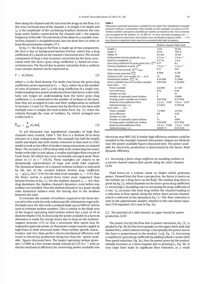
8132019 Efficiency of Tidal Turbine Farms
httpslidepdfcomreaderfullefficiency-of-tidal-turbine-farms 38
8132019 Efficiency of Tidal Turbine Farms
httpslidepdfcomreaderfullefficiency-of-tidal-turbine-farms 48
adding turbines decreases the power lost to the turbines ie C F u30
decreases as the bene1047297t of growing the farm to increase C F is out-
weighed by the reduction in u0 due to the additional drag Between
these two extremes there is a maximum power which can be lost
by the 1047298ow to the turbines (GC05) as seen in the power lost curves
in Fig 3b) This maximum power lost to the turbines P maxlost is
a channelrsquos potential which is the upper bound for how much
power a channel can generate The optimal gross farm drag coef-
1047297cient C F peak required to realize the potential can be estimated
from the analytic solution to GC05rsquos model using (V10-A4) or (V11-
210) To realize a channelrsquos potential P maxlost turbines must occupy
the entire cross-section Were it possible around 25 turbines would
1047297ll the cross-section of the shallow channel and 2500 the cross-
section of the tidal strait Table 1 Many turbines sweep a circular
area thus cannot 1047297ll a rectangular channelrsquos cross-section unless
contained within a square shroud Thus the number of turbines
required to 1047297ll the cross-section N 0 may not always be of practical
use However N 0 is a useful as a reference value for the size of a farm
in later discussions on turbine numbers where they only 1047297ll part of the cross-section or are spread amongst rows
GC05 found a remarkably simple approximate expression for
estimating the potential of a channel based on the transport
amplitude through the undisturbed channel U 0UD frac14 Au0 and the
amplitude of the headloss z0 which is given by
P maxlost frac14 022r g z0U 0UD (4)
[10] gives a method to estimate both the potential and the 1047298ow
speed reduction which only requires the transport along the
undisturbed channel which is easily measured using a vessel
mounted ADCP eg [18]
23 Gaps between turbines allows 1047298ow to bypass turbines reducing the power available for power production GC07
When there are wide gaps between turbines within a row to
allow for navigation some 1047298ow bypasses the turbines altogether
and does not contribute to power production The mixing of the
retarded 1047298ow passing through the turbines with the faster 1047298ow
passing around the turbines also dissipates some of the 1047298owrsquos
energy as heat [19] and GC07 The 1047298ows near a row of turbines
are shown schematically in Fig 2 GC07 extended classic
Lanchester-Betz actuator disc theory for an isolated turbine [2021]
to a row of turbines in a narrow channel Fig 2 They found that the
rowrsquos drag coef 1047297cient C R depends only on the blockage ratio ε the
fraction of the channelrsquos cross-sectional area occupied by the
turbines and the ratio r 3 frac14 u3=u which quanti1047297
es the 1047298
ow
reduction in the wake behind the turbines ie they found C Rethε r 3THORN
Though the functional relationship is complex and given in equa-
tions (GC07-223 V10-26) and (GC07-29 V10-27) for the purpose
of this work it is only essential to understand that the drag coef 1047297-
cient of a row only varies due tothe changes in the blockage ratio or
changes in the 1047298ow reduction behind the turbines C Rethε r 3THORN
increases as either ε is increased or the 1047298ow in the wake r 3 is
decreased The fraction of the cross-section occupied by the
turbines ie the blockage ratio is simply
ε frac14 M AT
A
where M is the number of turbines in the row AT is area blocked by
the rotating by the blades of a single turbine
The average power lost by the 1047298ow is given by Eq (3) This is not
the same as the power available to the turbine for electricity
production due to mixing losses behind the turbines GC05 and
[19] Using their results the power available is the smaller work
done by the 1047298ow through the turbine Fu1 whose average is
P avail frac14 4
3pr Ar 1N RC Ru3
0 (5)
where r 1 frac14 u1=u is the ratio of the velocity though the turbines to
the velocity upstream of the row Comparing Eqs (3) and (5) shows
that dueto mixing lossesonly thefraction r 1 of the power lostby the
1047298ow tothe turbines is available forelectricity productionwhere0
r 1 1 The power available Eq (5) represents an upper bound for
electricity which could be produced from a farm in a channel
24 Turbines must be adjusted or tuned for a particular channel
and in relation to each other to maximize the power available V10
amp V11
Maximizing the powerlost by the1047298owdue tothe farm Eq (3) is
not the same as maximizing the power available for generation as
they differ bya factorof r 1 Eq (5) Fig 3b) demonstrates this where
the power lost curve peaks at C F peak while the lower power
available curvespeak at a smallerdrag coef 1047297cient C F opt indicated by
the dots To maximize the power available the 1047298ow through the
turbines must be adjusted or tuned to give the optimal farm drag
coef 1047297cient C F opt Typically tuning is done by adjusting the pitch of
the turbinersquos blades Here this tuning is done mathematically by
adjusting the value of the 1047298ow reduction r 3 which affects both C Rand r 1 GC07
GC07rsquos extension of Lanchester-Betz theory to turbines in
a channel assumed the 1047298
ow upstream of the row u in Fig 2 was
0 05 1 1504
06
08
1
F l o w r e d u c t i o n
U 0
U 0 u n d i s t u r b e d
CF C
Fpeak
a
0 05 1 150
02
04
06
08
1
P o w e r P
m a x
CF C
Fpeak
Decreasing tuning parameter r3 minusgt
b
Fig 3 Effects of increasing farmrsquos drag coef 1047297cient for two example channels in Table 1 Solid lines are for shallow channel and dashed lines for tidal strait Horizontal axis is the farm
drag coef 1047297cient relative to the drag coef 1047297cient required to realize a channelrsquos potential ie at the peak in the power lost curve a) Reduction in 1047298ow relative to 1047298ow in undisturbed
channel b) Thick lines are the power lost to the turbines and thin lines are the power available from 5 rows of turbines in the shallow channel and 40 rows in the tidal strait when
turbines occupy 20 of the channel rsquos cross-section Solid dots show peak in power available curves at optimal tuning ie the upper bound for how much power is available from
these turbines
R Vennell Renewable Energy 47 (2012) 95e10298
8132019 Efficiency of Tidal Turbine Farms
httpslidepdfcomreaderfullefficiency-of-tidal-turbine-farms 58
1047297xed and found an optimal value of r 3 frac14 1=3 (equivalent to
r 1 frac14 2=3) which maximised the power available the same optimal
values as those for an isolated Lanchester-Betz turbine They also
found that at most 23 of the power lost to the turbines was
available for power production which occurred if the turbines took
up the minimum possible fraction of the cross-section However in
a channel with 1047298ows driven by head loss between its ends the 1047298ow
upstream of the row u isnot 1047297xed but decreases as the farmrsquos gross
drag coef 1047297cient C F frac14 N RC Rethε r 3THORN increases Thus C F depends on
the tuning r 3 Consequently changing the tuning changes the
strength of the 1047298ow along the entire channel via its effect on the
gross drag coef 1047297cient V10 V10 went on to show that a conse-
quence of this is that turbines need r 3 to be tuned to valuesbetween
13 and 1 to maximize the power available Thus tuning a large tidal
farm is very different from tuning a single isolated device A farmrsquos
optimal tuning r opt3 depends on a channelrsquos geometry and
dynamical balance as well as the blockage ratio ε V10 found that
by optimally tuning turbines it is possible to exceed GC07rsquos
maximum of 23 of a channelrsquos potential which is available for
power production
V11 went on toshow that not only does a row of turbinesneed to
betuned fora particularchannelit must also betuned in thepresence
of other rows tomaximizethe poweravailableThe needto tunerowsldquoin-concertrdquo has implications for modellers who must include
idealizedturbines in theirhydrodynamicmodelsto assess the power
available from a proposed site V11 and for the operators of turbine
farms as turbines come in and out of service Tuning in-concert may
require many model runs or complex interdependent adjustment of
operating turbines to 1047297nd the optimal set of turbine tunings The
need to tune turbines in-concert arises because rows of turbines in
narrow channels interact with each other via the farmrsquos gross drag
coef 1047297cient C F even if they are separated widely enough for the
disturbed 1047298ow through onerow tofullymix before encountering the
next row as C F affects 1047298ow along the entire channel
3 Farm and turbine ef 1047297ciency for a single row
31 Farm 1047298uid dynamic ef 1047297ciency
A measure of a farmrsquos ef 1047297ciency is the fraction of GC05rsquos
potential which is available for power production V10 ie
FE frac14 P avail
P maxlost
(6)
FEis the farmrsquos 1047298uid dynamic power ef 1047297ciency and is maximised
at the optimal tuning r opt3 V11 This is the headline ef 1047297ciency which
is theupper bound forthe fractionof a channelrsquos estimated potential
that can be turned into electricity from a given number of turbines
Fig 4a) shows FE for the two example channels as optimally
tuned turbines are added to a single row The curves for both
examples converge on 1 as turbines take up most of the cross-
section making most of the channelrsquos potential available for
power production For the shallow channel farm ef 1047297ciency initially
grows rapidly as turbines are added with reduced gains at higher
numbers indicating a diminishing return on additional turbines In
contrast for the tidal strait FE increases more rapidly at the higher
occupancies indicating an increasing return on new turbines added
to the row V11 Though a farm in the shallow channel is more
ef 1047297cient than the tidal strait for a given fraction of the cross-section
occupied in absolute terms the tidal strait has a much larger power
available and requires many more turbines to make up this given
fraction The thin lines in Fig 4a) show the reduction in 1047298ow speeds
due to adding turbines to the row Flow in the shallow channel
decreases more rapidly as turbines are added consistent with its
higher farm ef 1047297ciency
Fig 4a) shows the 1047297rst of two extreme ways to almost realise
a channelrsquos potential ie approach 100 farm ef 1047297ciency is to have
the optimally tuned turbines 1047297ll the cross-section ie blockage
ratio ε1 Turbines are normally thought of as extracting energy
from the 1047298owrsquos Kinetic Energy by reducing 1047298ows through the
turbines However paradoxically an optimally tuned tidal farm canalmost realise a channelrsquos potential without reducing the 1047298ow
through the turbines relative to the 1047298ow upstream ie the optimal
r 3 and r 11 as ε1 V10 The resolution lies in understanding the
source of the farmrsquos energy For an isolated turbine generation is
a result of reducing 1047298ows through the turbine where for a Betz
turbine the optimal tuning is r 3 frac14 1=3 corresponding to r 1 frac14 2=3
As the cross-section is 1047297lled with turbines the farmrsquos energy source
changes gradually from the 1047298owrsquos KE to the potential energy of the
1047298ow as optimal tunings increase So that at high blockage ratios the
energy source becomes the drop in water level between the
upstream and downstream sides of the farm ie the source is the
headloss across the farm It is also worth emphasizing that mixing
losses behind the turbines approach zero at high blockage ratios
which must happen if farm ef 1047297ciency is to approach 100 At highblockage ratios turbine farms approach an extreme form of a hydro-
electric dam with low head and high volume 1047298ow For the two
examples the head loss is only around 01 10 m while the peak
volume 1047298ows are 27 000 1 700 000 m3s1 In contrast a large
river dam has high head and low 1047298ow ie a 100 m head and
500 m3s1
32 Power available per turbine
Fig 4b) gives the power available per turbine as the cross-
sections are 1047297lled with turbines A single isolated turbine ε0
in the shallow channel makes 099 MW available per turbine
0 02 04 06 08 10
02
04
06
08
1
Fraction of crossminussection occupied ε
P a v a i l P m a x
o r U 0
U 0 U Da
F a r m
E f f i
c i e n c
y
F l o w r e d u c t i o n
0 02 04 06 08 10
05
1
15
2
Fraction of crossminussection occupied ε
P o w e r p e r t u r b i n e M Wb
Fig 4 Effect of the fraction of cross-section occupied by the turbines or blockage ratio on ef 1047297ciencies and 1047298ow speeds for a single row of optimally tuned turbines in a uniform
cross-section channel Solid curves are for shallow channel and dashed lines for tidal strait examples a) Thick lines are farm ef 1047297ciency Eq (6) the fraction of GC05rsquos potential which
is available for power production and thin lines 1047298
ow relative to undisturbed channel b) Power available per turbine in MW
R Vennell Renewable Energy 47 (2012) 95e102 99
8132019 Efficiency of Tidal Turbine Farms
httpslidepdfcomreaderfullefficiency-of-tidal-turbine-farms 68
whereas only 034 MW is available in the tidal strait due to much
weaker 1047298ows However as the cross-section is 1047297lled the power
available per turbine for the shallow channel decreases while for
the tidal strait power per turbine increases So paradoxically at
higher occupancies the tidal strait delivers up to six times more per
turbine despite having much weaker 1047298ows than the shallow
channel The curves in Fig 4b) are the result of two competing
effects Firstly occupying more of the cross-section increases
a rowrsquos drag coef 1047297cient C R increases the power available Eq (5)
Secondly increasing a rows drag coef 1047297cient reduces the 1047298ow along
the channel U 0 which acts to decrease the power available in Eq
(5) The net effect differs for the two examples For the shallow
channel the more rapid reduction in 1047298ow speed as the cross-section
is 1047297lled Fig 4a) outweighs the enhanced drag coef 1047297cient leading
to reduction in the power per turbine from 099 MW to only
036 MW at high occupancy In contrast the more gradual 1047298ow
reduction in the tidal strait leads to an increasing power available
per turbine as the cross-section is 1047297lledfrom 034MW to23MW A
result is that above 35 occupancy the tidal strait delivers more per
turbine than the shallow channel despite the much weaker 1047298ows in
the strait
The differing performance of the turbines as the cross-section is
1047297lled is linked to their differing dynamical balances At higheroccupancies in the shallow channel the power lost to the turbines is
similar to that lost to background friction (this can be inferred from
(V10-A4) where C F peak is around twice the scaled background
bottom friction coef 1047297cient C D for near steady state channels ie
large l0 channels) This signi1047297cant energy loss to bottom friction
and turbine drag is associated with a more rapid decrease in 1047298ows
a diminishing return on new turbines and the decreasing power
available per turbine in Fig 4 In contrast in the tidal strait bottom
friction is almost unimportant and relatively little energy is lost to
bottom friction This gives the strait a proportionately higher
potential and an increasing return on additional turbines as they
becomemore ef 1047297cient when occupying more of the cross-section of
the ldquoductrdquo formed by the channel The energetics of channels with
turbine farms is discussed in detail in [17]
4 Ef 1047297ciency of multi-row farms
Adding capacity to a farm by adding rows of optimally tuned
turbines increases farm ef 1047297ciency as demonstrated in Fig 5a) For
the tidal strait 15 rows makes only 40 of it potential available so as
would be expected the associated 1047298ow reduction is modest In
contrast for the shallow channel 3 rows make 70 of its potential
available with a signi1047297cant associated 1047298ow reduction
Fig 5 illustrates a second extreme way to realize most of
a channelrsquos potential having a large number of rows However for
both channels there is a diminishing return on additional rows
Farm ef 1047297ciency peaks at a very large number of rows indicating an
optimal farm size However the diminishing return on new rows is
so harsh near this peak that farm size will be restricted to a much
smaller of number rows [17] V11 showed that for two similar
examples the best strategy for growing a farm of optimally tuned
turbines is the intuitive one Fill the 1047297rst row up to the maximum
permitted by navigational constraints and then add rows up to
a maximum that can be economically justi1047297ed in the light of the
diminishing returns inherent in Fig 5a)
5 Realizing the potential a trade off
The decision on turbine numbers is an economic trade off
between the income from the power made available by adding
turbines to a farm against their cost and any environmental
impacts Once the maximum permissible cross-sectional occu-
pancy has been achieved then the trade off is in the face of
a diminishing return on additional turbines Fig 5a) How this trade
off plays out depends strongly on the maximum fraction of the
channelrsquos cross-section which can be occupied in order to maintain
navigation along the channel It also strongly depends on the
dynamical balance of the undisturbed channel be it that of
a bottom friction dominated shallow channel or that of an inertia
dominated tidal strait Fig 5
This diminishing return is inherent in the upper row of plots in
Fig 6 where for both a low cross-sectional occupancy ε frac14 01 and
what may be an unrealistically high occupancy ε frac14 05 power
available increases more slowly as rows are added to an optimally
tuned farm While the ultimate choice on number of turbines
comes down to an economic and environmental cost bene1047297t
analysis which is beyond the scope of this work the plots however
do contain essential information to underpin this analysis For the
shallow channel at the high occupancy 1 row of 12 turbines makes
80 of its 9 MW potential available Fig 6a) In contrast the same
number of turbines spread across 5 rows at the lower occupancy
makes only 65 of the potential available for power productionFig 6c) shows that the power available per turbine for both occu-
pancies decreases as rows are added Fig 6e) illustrates that for
both occupancies a farm making 80 of the shallow channelrsquos
potential available will reduce 1047298ows by 30 If such a signi1047297cant
1047298ow reduction is not acceptable then at the lower occupancy
installing around 3 turbines reduces 1047298ows by only 10 while
making around 25 of its potential available
The curves for the tidal strait in Fig 6b) d) and f) are similar to
those of the shallow channel but the number of turbines involved
is much larger Almost 80 of the straitrsquos 6 GW potential can be
realized at the higher occupancy but this requires an astonishing
0 5 10 150
02
04
06
08
1
Number of Rows NR
a
Farm Efficiency
0 5 10 1504
06
08
1
Number of Rows NR
b
Flow reduction
Fig 5 Effect of adding rows to an optimally tuned farm where turbines occupy 20 of the channel rsquos cross-section ie a blockage ratio of ε frac14 02 Solid curves are for the shallow
channel and dashed lines for the tidal strait a) Farm ef 1047297
ciency Eq (6) b) Velocity relative to undisturbed velocity
R Vennell Renewable Energy 47 (2012) 95e102100
8132019 Efficiency of Tidal Turbine Farms
httpslidepdfcomreaderfullefficiency-of-tidal-turbine-farms 78
16000 turbines spread over 13 rows At the lower occupancy
a more affordable 5000 turbines would make 30 of the strait rsquos
potential available while reducing 1047298ows by 7
6 Discussion
The principle aim of this paper was to show how many turbines
are required to realize a given fraction of a channel rsquos potential in
order to improve understanding of how power production scales
with farm size The models in V10 and V11 which build on those of
GC05 and GC07 provide the 1047297rst physically coherent way of con-
necting the number of turbines in a farm with the maximum power
available for electricity production The models do not require the
use of arbitrary loading or safety factors applied to account for
unknown effects The models are however simple They use an
extended form of classic turbine theory and they only apply to the
cross-sectional average velocities thusdo not account for the effects
of any variation of 1047298ow across the channel or with depth They also
do not allow for any effect of the turbulence shed by a row on the
ef 1047297
ciency of downstream rows They do not allow for minimum
turbine operating 1047298ows or for loss due to their electro-mechanical
ef 1047297ciency or transmission and conversion losses Thus there is
muchworktobedonetore1047297ne and extend the modelsHowever the
models do illuminate signi1047297cant aspects of developing large tidal
turbine farms Most of these are a result of power extraction
reducing the 1047298ows along the entire narrow channel via the farmrsquos
gross dragcoef 1047297cient C F They include thenecessity totune turbines
for the particular channel and in relation to each other which will
result in signi1047297cant computational cost to those modelling turbine
farms and will require on going optimization of turbine tuning in
large operational farms as turbines come in and out of service They
also include how farms have increasing or diminishing returns on
turbines added to thecross-section dependingon the importance of
bottom friction and how there is always a diminishing return on
additional rows aspects which are fundamental to understanding
the economics of farm development
The turbine numbers given by the simple models should be
viewed as estimates of the magnitude of the numbers required
rather than precise estimates These magnitudes are useful in
understanding how realistic it is to realize a signi1047297
cant fraction of
0 10 20 30 400
02
04
06
08
1
1
3
5
101
3
P o w e r P
m a x
Number of Turbines
aShallow Channel
0 5 10 150
02
04
06
08
1
1
5
10
20
50
1
5
10
P o w e r P
m a x
Thousands of Turbines
bTidal Strait
0 10 20 30 400
02
04
06
08
1
12
P o w
e r P e r T u r b i n e M W
Number of Turbines
c
0 5 100
02
04
06
08
1
12
P o w
e r P e r T u r b i n e M W
Thousands of Turbines
d
06 07 08 09 10
02
04
06
08
1
5
10
15
2515
25
P o w e r P
m a x
Flow Reduction
e
06 07 08 09 10
02
04
06
08
1
10002000
5000
10000
15000
2000
5000
10000
15000
P o w e r P
m a x
Flow Reduction
f
Fig 6 Effect of the number of optimally tuned turbines on power available and 1047298ow reduction for the two example channels based on a 400 m 2 blade area Solid curves are for
ε frac14 01 and dashed lines for ε frac14 05 a) and b) Farm ef 1047297ciency versus number of turbines labelled dots give number of rows in the farm c) and d) Power available per turbine in
MW e) and f) Farm ef 1047297ciency verses 1047298ow reduction Labelled dots give the number of turbines in farm
R Vennell Renewable Energy 47 (2012) 95e102 101
8132019 Efficiency of Tidal Turbine Farms
httpslidepdfcomreaderfullefficiency-of-tidal-turbine-farms 88
a channelrsquos potential For the shallow channel around eight 400 m2
turbines corresponding to three rows with ε frac14 01 makes half of
its potential available and 13 corresponding to one row with
ε frac14 05 makes 80 available Table 1 The given values for the
power available per turbine are also useful in understanding
economic feasibility For blockage ratios of ε frac14 01 and 05 each
turbine makes around 06 MW available The detailed economics
and environmental costs are beyond the scope of this work
however making an average of 06 MWavailable over the tidal cycle
when existing turbines are producing around 1 MW at steady1047298ows
around2 m s1 maybe a reasonable return Thus it appears possible
to make a signi1047297cant fraction of the shallow channelrsquos potential
available using 5e10 turbines with a blade area similar to that of
the largest currently operating tidal turbine spread amongst 1e3
rows which occupy less than 50 of the cross-section
In contrast to make 50 of the tidal straitrsquos 6 GW potential
available takes 10000 turbines at 10 blockage This high number
is a result of the weaker 1047298ows in the tidal strait which yield only
027 MW per turbine However unlike the tidal shallow channel
the output per turbine rises as more of the strait rsquos cross-section is
occupied So that at 50 blockage only 5000 turbines are required
to make 50 of its potentialavailable at a much higher 061MW per
turbine similar to that for the shallow channel Tidal straits haveboth a much larger potential in absolute terms and in proportion to
their size due to relatively low energy losses to bottom friction
This is seen in their having six times the potential per turbinewhen
turbines 1047297ll the cross-section in a single row Table 1 However tidal
straits typically have weaker cross-sectionally averaged 1047298ows than
shallow tidal channels Thus at low blockage ratios a very large
number of rows are required to make a signi1047297cant fraction avail-
able If higher blockage ratios are permitted then the enhanced
ef 1047297ciency of turbines in tidal straits seen in Fig 4 boosts the output
per turbine and reduces the total number of turbines required [17]
uses the channelrsquos energy balance to explain why and when tidal
straits have an increasing return on turbines added to the cross-
section and why shallow channels have a diminishing return
7 Conclusions
Critical questions in developing a farm are what fraction of
a channelrsquos potential is available for power production from a given
number of turbines as a farm scales up from a single turbine into
a large farm The V10 thorn V11 works provide the 1047297rst physically
coherent way to connect the number of turbines in a farm to both
the maximum power available for electricity production and to the
degree of 1047298ow reduction which is a consequence of power
extraction Though simple they illuminate several important
aspects of developing large farms which have implications for both
the economics and environmental impact of farms Such as the
necessity of tuning turbines in large farms for the particular
channel how much of the cross-section they occupy and the
number of rows as well as how to best arrange and con1047297gure the
turbines For example to maximize farm ef 1047297ciency the 1047297rst row
turbines should be 1047297lled up to the maximum permitted by navi-
gational constraints before adding new rows Also while farm
ef 1047297ciency always increases as optimally tuned turbines are added
once the cross-sectional occupancy limit is attained the power
available per turbine decreases as rows are added Thus increasing
power production by increasing the farmrsquos installed capacity faces
a diminishing return on additional rows This development strategy
may alter when more realistic models are developed which allow
for variation of 1047298ow across the channel and with depth However
the decision on turbine numbers will remain an economic trade off
between the power produced and installation maintenance and
environmental costs How this trade off plays out depends strongly
on the maximum fraction of the channelrsquos cross-section which can
be occupied and the dynamical balance of the undisturbed channel
The examples demonstrate that it may be possible with existing
technology to realize much of the MW potential of shallow tidal
channels The GW potential of tidal straits is both larger in absolute
terms and also proportionately larger than that of shallow chan-
nels due to relatively low energy losses to bottom friction At low
cross-sectional occupancies the typically lower 1047298ows of the strait
result in both a low return per turbine and a very large number of
turbines being required to realize a signi1047297cant fraction of their
proportionately higher potential Thus unless a large fraction of the
straitrsquos cross-section can be occupied to take advantage of a higher
output per turbine it will be dif 1047297cult to realize a substantial frac-
tion of the GW potential of tidal straits until larger turbines are
developed which are able operate economically in low 1047298ows
References
[1] Garrett C Cummins P The power potential of tidal currents in channels
Proceedings of the Royal Society A 20054612563e
72[2] Blunden LS Bahaj AS Tidal energy resource assessment for tidal stream
generators Proceedings of the Institution of Mechanical Engineers Part A Journal of Power and Energy 2007221(10)137e46 doi10124309576509JPE332
[3] Blanch1047297eld J Garrett C Rowe A Wild P Tidal stream power resourceassessment for Masset Sound Haida Gwaii Proceedings of the Institution of Mechanical Engineers Part A Journal of Power and Energy 2008222(5)485e92
[4] Neill SP Litt EJ Couch SJ Davies AG The impact of tidal stream turbines onlarge-scale sediment dynamics Renewable Energy 200934(12)2803e12doi101016jrenene200906015
[5] Garrett C Cummins P Limits to tidal current power Renewable Energy 2008332485e90
[6] Garrett C Cummins P Tuning turbines in a tidal channel Journal of FluidMechanics 2010663253e67 doi101017S0022112010003502
[7] Vennell R Tuning tidal turbines in concert to maximise farm ef 1047297ciency Journal of Fluid Mechanics 2011671587e604
[8] Garrett C Cummins P The ef 1047297
ciency of a turbine in a tidal channel Journal of Fluid Mechanics 2007588243e51[9] Blanch1047297eld J Garrett C Wild P Rowe A The extractable power from a channel
linking a bay to the open ocean Proceedings of the Institution of MechanicalEngineers Part A Journal of Power and Energy 2008222(3)289e97
[10] Vennell R Estimating the power potential of tidal currents and the impact of power extraction on 1047298ow speeds Renewable Energy 2011363558e65 doi101016jrenene201105011
[11] Arbic B Garrett C A coupled oscillator model of shelf and ocean tidesContinental Shelf Research 201030(6)564e74
[12] Vennell R Oscillating barotropic currents along short channels Journal of Physical Oceanography 199828(8)1561e9
[13] Vennell R Observations of the phase of tidal currents along a strait Journal of Physical Oceanography 199828(8)1570e7
[14] Byden IG Grinsted T Melville GT Assessing the potential of a simple tidalchannel to deliver useful energy Journal of Applied Ocean Research 200426198e204 doi101016japor200504001
[15] Vennell R ADCP measurements of tidal phase and amplitude in Cook StraitNew Zealand Continental Shelf Research 199414353e64
[16] Douglas C Harrison G Chick J Life cycle assessment of the Seagen marinecurrent turbine Proceedings of the Institution of Mechanical Engineers Part M
Journal of Engineering for the Maritime Environment 2008222(1)1e12 doi10124314750902JEME94
[17] Vennell R The energetics of large tidal turbine arrays Renewable Energyin press
[18] Vennell R ADCP measurements of momentum balance and dynamic topog-raphy in a constricted tidal channel Journal of Physical Oceanography 200636(2)177e88
[19] Corten G Heat generation by a wind turbine Vol In 14th IEA symposium onthe aerodynamics of wind turbines 2000 p 7 ECN report ECN-RX-01-001
[20] Lanchester FW A contribution to the theory of propulsion and the screwpropeller Transactions of the Institution of Naval Architects 1915LVII98e116
[21] Betz A Das Maximum der theoretisch moumlglichen Ausnutzung des Windesdurch Windmotoren Gesamte Turbinenwesen 192017307e9
R Vennell Renewable Energy 47 (2012) 95e102102
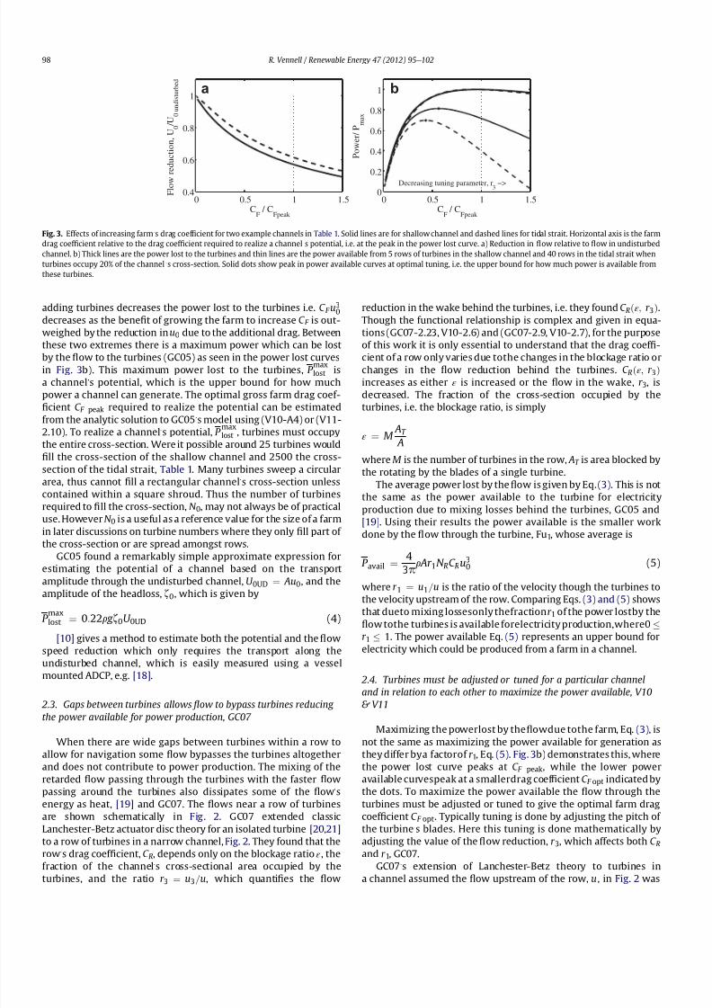
8132019 Efficiency of Tidal Turbine Farms
httpslidepdfcomreaderfullefficiency-of-tidal-turbine-farms 48
adding turbines decreases the power lost to the turbines ie C F u30
decreases as the bene1047297t of growing the farm to increase C F is out-
weighed by the reduction in u0 due to the additional drag Between
these two extremes there is a maximum power which can be lost
by the 1047298ow to the turbines (GC05) as seen in the power lost curves
in Fig 3b) This maximum power lost to the turbines P maxlost is
a channelrsquos potential which is the upper bound for how much
power a channel can generate The optimal gross farm drag coef-
1047297cient C F peak required to realize the potential can be estimated
from the analytic solution to GC05rsquos model using (V10-A4) or (V11-
210) To realize a channelrsquos potential P maxlost turbines must occupy
the entire cross-section Were it possible around 25 turbines would
1047297ll the cross-section of the shallow channel and 2500 the cross-
section of the tidal strait Table 1 Many turbines sweep a circular
area thus cannot 1047297ll a rectangular channelrsquos cross-section unless
contained within a square shroud Thus the number of turbines
required to 1047297ll the cross-section N 0 may not always be of practical
use However N 0 is a useful as a reference value for the size of a farm
in later discussions on turbine numbers where they only 1047297ll part of the cross-section or are spread amongst rows
GC05 found a remarkably simple approximate expression for
estimating the potential of a channel based on the transport
amplitude through the undisturbed channel U 0UD frac14 Au0 and the
amplitude of the headloss z0 which is given by
P maxlost frac14 022r g z0U 0UD (4)
[10] gives a method to estimate both the potential and the 1047298ow
speed reduction which only requires the transport along the
undisturbed channel which is easily measured using a vessel
mounted ADCP eg [18]
23 Gaps between turbines allows 1047298ow to bypass turbines reducing the power available for power production GC07
When there are wide gaps between turbines within a row to
allow for navigation some 1047298ow bypasses the turbines altogether
and does not contribute to power production The mixing of the
retarded 1047298ow passing through the turbines with the faster 1047298ow
passing around the turbines also dissipates some of the 1047298owrsquos
energy as heat [19] and GC07 The 1047298ows near a row of turbines
are shown schematically in Fig 2 GC07 extended classic
Lanchester-Betz actuator disc theory for an isolated turbine [2021]
to a row of turbines in a narrow channel Fig 2 They found that the
rowrsquos drag coef 1047297cient C R depends only on the blockage ratio ε the
fraction of the channelrsquos cross-sectional area occupied by the
turbines and the ratio r 3 frac14 u3=u which quanti1047297
es the 1047298
ow
reduction in the wake behind the turbines ie they found C Rethε r 3THORN
Though the functional relationship is complex and given in equa-
tions (GC07-223 V10-26) and (GC07-29 V10-27) for the purpose
of this work it is only essential to understand that the drag coef 1047297-
cient of a row only varies due tothe changes in the blockage ratio or
changes in the 1047298ow reduction behind the turbines C Rethε r 3THORN
increases as either ε is increased or the 1047298ow in the wake r 3 is
decreased The fraction of the cross-section occupied by the
turbines ie the blockage ratio is simply
ε frac14 M AT
A
where M is the number of turbines in the row AT is area blocked by
the rotating by the blades of a single turbine
The average power lost by the 1047298ow is given by Eq (3) This is not
the same as the power available to the turbine for electricity
production due to mixing losses behind the turbines GC05 and
[19] Using their results the power available is the smaller work
done by the 1047298ow through the turbine Fu1 whose average is
P avail frac14 4
3pr Ar 1N RC Ru3
0 (5)
where r 1 frac14 u1=u is the ratio of the velocity though the turbines to
the velocity upstream of the row Comparing Eqs (3) and (5) shows
that dueto mixing lossesonly thefraction r 1 of the power lostby the
1047298ow tothe turbines is available forelectricity productionwhere0
r 1 1 The power available Eq (5) represents an upper bound for
electricity which could be produced from a farm in a channel
24 Turbines must be adjusted or tuned for a particular channel
and in relation to each other to maximize the power available V10
amp V11
Maximizing the powerlost by the1047298owdue tothe farm Eq (3) is
not the same as maximizing the power available for generation as
they differ bya factorof r 1 Eq (5) Fig 3b) demonstrates this where
the power lost curve peaks at C F peak while the lower power
available curvespeak at a smallerdrag coef 1047297cient C F opt indicated by
the dots To maximize the power available the 1047298ow through the
turbines must be adjusted or tuned to give the optimal farm drag
coef 1047297cient C F opt Typically tuning is done by adjusting the pitch of
the turbinersquos blades Here this tuning is done mathematically by
adjusting the value of the 1047298ow reduction r 3 which affects both C Rand r 1 GC07
GC07rsquos extension of Lanchester-Betz theory to turbines in
a channel assumed the 1047298
ow upstream of the row u in Fig 2 was
0 05 1 1504
06
08
1
F l o w r e d u c t i o n
U 0
U 0 u n d i s t u r b e d
CF C
Fpeak
a
0 05 1 150
02
04
06
08
1
P o w e r P
m a x
CF C
Fpeak
Decreasing tuning parameter r3 minusgt
b
Fig 3 Effects of increasing farmrsquos drag coef 1047297cient for two example channels in Table 1 Solid lines are for shallow channel and dashed lines for tidal strait Horizontal axis is the farm
drag coef 1047297cient relative to the drag coef 1047297cient required to realize a channelrsquos potential ie at the peak in the power lost curve a) Reduction in 1047298ow relative to 1047298ow in undisturbed
channel b) Thick lines are the power lost to the turbines and thin lines are the power available from 5 rows of turbines in the shallow channel and 40 rows in the tidal strait when
turbines occupy 20 of the channel rsquos cross-section Solid dots show peak in power available curves at optimal tuning ie the upper bound for how much power is available from
these turbines
R Vennell Renewable Energy 47 (2012) 95e10298
8132019 Efficiency of Tidal Turbine Farms
httpslidepdfcomreaderfullefficiency-of-tidal-turbine-farms 58
1047297xed and found an optimal value of r 3 frac14 1=3 (equivalent to
r 1 frac14 2=3) which maximised the power available the same optimal
values as those for an isolated Lanchester-Betz turbine They also
found that at most 23 of the power lost to the turbines was
available for power production which occurred if the turbines took
up the minimum possible fraction of the cross-section However in
a channel with 1047298ows driven by head loss between its ends the 1047298ow
upstream of the row u isnot 1047297xed but decreases as the farmrsquos gross
drag coef 1047297cient C F frac14 N RC Rethε r 3THORN increases Thus C F depends on
the tuning r 3 Consequently changing the tuning changes the
strength of the 1047298ow along the entire channel via its effect on the
gross drag coef 1047297cient V10 V10 went on to show that a conse-
quence of this is that turbines need r 3 to be tuned to valuesbetween
13 and 1 to maximize the power available Thus tuning a large tidal
farm is very different from tuning a single isolated device A farmrsquos
optimal tuning r opt3 depends on a channelrsquos geometry and
dynamical balance as well as the blockage ratio ε V10 found that
by optimally tuning turbines it is possible to exceed GC07rsquos
maximum of 23 of a channelrsquos potential which is available for
power production
V11 went on toshow that not only does a row of turbinesneed to
betuned fora particularchannelit must also betuned in thepresence
of other rows tomaximizethe poweravailableThe needto tunerowsldquoin-concertrdquo has implications for modellers who must include
idealizedturbines in theirhydrodynamicmodelsto assess the power
available from a proposed site V11 and for the operators of turbine
farms as turbines come in and out of service Tuning in-concert may
require many model runs or complex interdependent adjustment of
operating turbines to 1047297nd the optimal set of turbine tunings The
need to tune turbines in-concert arises because rows of turbines in
narrow channels interact with each other via the farmrsquos gross drag
coef 1047297cient C F even if they are separated widely enough for the
disturbed 1047298ow through onerow tofullymix before encountering the
next row as C F affects 1047298ow along the entire channel
3 Farm and turbine ef 1047297ciency for a single row
31 Farm 1047298uid dynamic ef 1047297ciency
A measure of a farmrsquos ef 1047297ciency is the fraction of GC05rsquos
potential which is available for power production V10 ie
FE frac14 P avail
P maxlost
(6)
FEis the farmrsquos 1047298uid dynamic power ef 1047297ciency and is maximised
at the optimal tuning r opt3 V11 This is the headline ef 1047297ciency which
is theupper bound forthe fractionof a channelrsquos estimated potential
that can be turned into electricity from a given number of turbines
Fig 4a) shows FE for the two example channels as optimally
tuned turbines are added to a single row The curves for both
examples converge on 1 as turbines take up most of the cross-
section making most of the channelrsquos potential available for
power production For the shallow channel farm ef 1047297ciency initially
grows rapidly as turbines are added with reduced gains at higher
numbers indicating a diminishing return on additional turbines In
contrast for the tidal strait FE increases more rapidly at the higher
occupancies indicating an increasing return on new turbines added
to the row V11 Though a farm in the shallow channel is more
ef 1047297cient than the tidal strait for a given fraction of the cross-section
occupied in absolute terms the tidal strait has a much larger power
available and requires many more turbines to make up this given
fraction The thin lines in Fig 4a) show the reduction in 1047298ow speeds
due to adding turbines to the row Flow in the shallow channel
decreases more rapidly as turbines are added consistent with its
higher farm ef 1047297ciency
Fig 4a) shows the 1047297rst of two extreme ways to almost realise
a channelrsquos potential ie approach 100 farm ef 1047297ciency is to have
the optimally tuned turbines 1047297ll the cross-section ie blockage
ratio ε1 Turbines are normally thought of as extracting energy
from the 1047298owrsquos Kinetic Energy by reducing 1047298ows through the
turbines However paradoxically an optimally tuned tidal farm canalmost realise a channelrsquos potential without reducing the 1047298ow
through the turbines relative to the 1047298ow upstream ie the optimal
r 3 and r 11 as ε1 V10 The resolution lies in understanding the
source of the farmrsquos energy For an isolated turbine generation is
a result of reducing 1047298ows through the turbine where for a Betz
turbine the optimal tuning is r 3 frac14 1=3 corresponding to r 1 frac14 2=3
As the cross-section is 1047297lled with turbines the farmrsquos energy source
changes gradually from the 1047298owrsquos KE to the potential energy of the
1047298ow as optimal tunings increase So that at high blockage ratios the
energy source becomes the drop in water level between the
upstream and downstream sides of the farm ie the source is the
headloss across the farm It is also worth emphasizing that mixing
losses behind the turbines approach zero at high blockage ratios
which must happen if farm ef 1047297ciency is to approach 100 At highblockage ratios turbine farms approach an extreme form of a hydro-
electric dam with low head and high volume 1047298ow For the two
examples the head loss is only around 01 10 m while the peak
volume 1047298ows are 27 000 1 700 000 m3s1 In contrast a large
river dam has high head and low 1047298ow ie a 100 m head and
500 m3s1
32 Power available per turbine
Fig 4b) gives the power available per turbine as the cross-
sections are 1047297lled with turbines A single isolated turbine ε0
in the shallow channel makes 099 MW available per turbine
0 02 04 06 08 10
02
04
06
08
1
Fraction of crossminussection occupied ε
P a v a i l P m a x
o r U 0
U 0 U Da
F a r m
E f f i
c i e n c
y
F l o w r e d u c t i o n
0 02 04 06 08 10
05
1
15
2
Fraction of crossminussection occupied ε
P o w e r p e r t u r b i n e M Wb
Fig 4 Effect of the fraction of cross-section occupied by the turbines or blockage ratio on ef 1047297ciencies and 1047298ow speeds for a single row of optimally tuned turbines in a uniform
cross-section channel Solid curves are for shallow channel and dashed lines for tidal strait examples a) Thick lines are farm ef 1047297ciency Eq (6) the fraction of GC05rsquos potential which
is available for power production and thin lines 1047298
ow relative to undisturbed channel b) Power available per turbine in MW
R Vennell Renewable Energy 47 (2012) 95e102 99
8132019 Efficiency of Tidal Turbine Farms
httpslidepdfcomreaderfullefficiency-of-tidal-turbine-farms 68
whereas only 034 MW is available in the tidal strait due to much
weaker 1047298ows However as the cross-section is 1047297lled the power
available per turbine for the shallow channel decreases while for
the tidal strait power per turbine increases So paradoxically at
higher occupancies the tidal strait delivers up to six times more per
turbine despite having much weaker 1047298ows than the shallow
channel The curves in Fig 4b) are the result of two competing
effects Firstly occupying more of the cross-section increases
a rowrsquos drag coef 1047297cient C R increases the power available Eq (5)
Secondly increasing a rows drag coef 1047297cient reduces the 1047298ow along
the channel U 0 which acts to decrease the power available in Eq
(5) The net effect differs for the two examples For the shallow
channel the more rapid reduction in 1047298ow speed as the cross-section
is 1047297lled Fig 4a) outweighs the enhanced drag coef 1047297cient leading
to reduction in the power per turbine from 099 MW to only
036 MW at high occupancy In contrast the more gradual 1047298ow
reduction in the tidal strait leads to an increasing power available
per turbine as the cross-section is 1047297lledfrom 034MW to23MW A
result is that above 35 occupancy the tidal strait delivers more per
turbine than the shallow channel despite the much weaker 1047298ows in
the strait
The differing performance of the turbines as the cross-section is
1047297lled is linked to their differing dynamical balances At higheroccupancies in the shallow channel the power lost to the turbines is
similar to that lost to background friction (this can be inferred from
(V10-A4) where C F peak is around twice the scaled background
bottom friction coef 1047297cient C D for near steady state channels ie
large l0 channels) This signi1047297cant energy loss to bottom friction
and turbine drag is associated with a more rapid decrease in 1047298ows
a diminishing return on new turbines and the decreasing power
available per turbine in Fig 4 In contrast in the tidal strait bottom
friction is almost unimportant and relatively little energy is lost to
bottom friction This gives the strait a proportionately higher
potential and an increasing return on additional turbines as they
becomemore ef 1047297cient when occupying more of the cross-section of
the ldquoductrdquo formed by the channel The energetics of channels with
turbine farms is discussed in detail in [17]
4 Ef 1047297ciency of multi-row farms
Adding capacity to a farm by adding rows of optimally tuned
turbines increases farm ef 1047297ciency as demonstrated in Fig 5a) For
the tidal strait 15 rows makes only 40 of it potential available so as
would be expected the associated 1047298ow reduction is modest In
contrast for the shallow channel 3 rows make 70 of its potential
available with a signi1047297cant associated 1047298ow reduction
Fig 5 illustrates a second extreme way to realize most of
a channelrsquos potential having a large number of rows However for
both channels there is a diminishing return on additional rows
Farm ef 1047297ciency peaks at a very large number of rows indicating an
optimal farm size However the diminishing return on new rows is
so harsh near this peak that farm size will be restricted to a much
smaller of number rows [17] V11 showed that for two similar
examples the best strategy for growing a farm of optimally tuned
turbines is the intuitive one Fill the 1047297rst row up to the maximum
permitted by navigational constraints and then add rows up to
a maximum that can be economically justi1047297ed in the light of the
diminishing returns inherent in Fig 5a)
5 Realizing the potential a trade off
The decision on turbine numbers is an economic trade off
between the income from the power made available by adding
turbines to a farm against their cost and any environmental
impacts Once the maximum permissible cross-sectional occu-
pancy has been achieved then the trade off is in the face of
a diminishing return on additional turbines Fig 5a) How this trade
off plays out depends strongly on the maximum fraction of the
channelrsquos cross-section which can be occupied in order to maintain
navigation along the channel It also strongly depends on the
dynamical balance of the undisturbed channel be it that of
a bottom friction dominated shallow channel or that of an inertia
dominated tidal strait Fig 5
This diminishing return is inherent in the upper row of plots in
Fig 6 where for both a low cross-sectional occupancy ε frac14 01 and
what may be an unrealistically high occupancy ε frac14 05 power
available increases more slowly as rows are added to an optimally
tuned farm While the ultimate choice on number of turbines
comes down to an economic and environmental cost bene1047297t
analysis which is beyond the scope of this work the plots however
do contain essential information to underpin this analysis For the
shallow channel at the high occupancy 1 row of 12 turbines makes
80 of its 9 MW potential available Fig 6a) In contrast the same
number of turbines spread across 5 rows at the lower occupancy
makes only 65 of the potential available for power productionFig 6c) shows that the power available per turbine for both occu-
pancies decreases as rows are added Fig 6e) illustrates that for
both occupancies a farm making 80 of the shallow channelrsquos
potential available will reduce 1047298ows by 30 If such a signi1047297cant
1047298ow reduction is not acceptable then at the lower occupancy
installing around 3 turbines reduces 1047298ows by only 10 while
making around 25 of its potential available
The curves for the tidal strait in Fig 6b) d) and f) are similar to
those of the shallow channel but the number of turbines involved
is much larger Almost 80 of the straitrsquos 6 GW potential can be
realized at the higher occupancy but this requires an astonishing
0 5 10 150
02
04
06
08
1
Number of Rows NR
a
Farm Efficiency
0 5 10 1504
06
08
1
Number of Rows NR
b
Flow reduction
Fig 5 Effect of adding rows to an optimally tuned farm where turbines occupy 20 of the channel rsquos cross-section ie a blockage ratio of ε frac14 02 Solid curves are for the shallow
channel and dashed lines for the tidal strait a) Farm ef 1047297
ciency Eq (6) b) Velocity relative to undisturbed velocity
R Vennell Renewable Energy 47 (2012) 95e102100
8132019 Efficiency of Tidal Turbine Farms
httpslidepdfcomreaderfullefficiency-of-tidal-turbine-farms 78
16000 turbines spread over 13 rows At the lower occupancy
a more affordable 5000 turbines would make 30 of the strait rsquos
potential available while reducing 1047298ows by 7
6 Discussion
The principle aim of this paper was to show how many turbines
are required to realize a given fraction of a channel rsquos potential in
order to improve understanding of how power production scales
with farm size The models in V10 and V11 which build on those of
GC05 and GC07 provide the 1047297rst physically coherent way of con-
necting the number of turbines in a farm with the maximum power
available for electricity production The models do not require the
use of arbitrary loading or safety factors applied to account for
unknown effects The models are however simple They use an
extended form of classic turbine theory and they only apply to the
cross-sectional average velocities thusdo not account for the effects
of any variation of 1047298ow across the channel or with depth They also
do not allow for any effect of the turbulence shed by a row on the
ef 1047297
ciency of downstream rows They do not allow for minimum
turbine operating 1047298ows or for loss due to their electro-mechanical
ef 1047297ciency or transmission and conversion losses Thus there is
muchworktobedonetore1047297ne and extend the modelsHowever the
models do illuminate signi1047297cant aspects of developing large tidal
turbine farms Most of these are a result of power extraction
reducing the 1047298ows along the entire narrow channel via the farmrsquos
gross dragcoef 1047297cient C F They include thenecessity totune turbines
for the particular channel and in relation to each other which will
result in signi1047297cant computational cost to those modelling turbine
farms and will require on going optimization of turbine tuning in
large operational farms as turbines come in and out of service They
also include how farms have increasing or diminishing returns on
turbines added to thecross-section dependingon the importance of
bottom friction and how there is always a diminishing return on
additional rows aspects which are fundamental to understanding
the economics of farm development
The turbine numbers given by the simple models should be
viewed as estimates of the magnitude of the numbers required
rather than precise estimates These magnitudes are useful in
understanding how realistic it is to realize a signi1047297
cant fraction of
0 10 20 30 400
02
04
06
08
1
1
3
5
101
3
P o w e r P
m a x
Number of Turbines
aShallow Channel
0 5 10 150
02
04
06
08
1
1
5
10
20
50
1
5
10
P o w e r P
m a x
Thousands of Turbines
bTidal Strait
0 10 20 30 400
02
04
06
08
1
12
P o w
e r P e r T u r b i n e M W
Number of Turbines
c
0 5 100
02
04
06
08
1
12
P o w
e r P e r T u r b i n e M W
Thousands of Turbines
d
06 07 08 09 10
02
04
06
08
1
5
10
15
2515
25
P o w e r P
m a x
Flow Reduction
e
06 07 08 09 10
02
04
06
08
1
10002000
5000
10000
15000
2000
5000
10000
15000
P o w e r P
m a x
Flow Reduction
f
Fig 6 Effect of the number of optimally tuned turbines on power available and 1047298ow reduction for the two example channels based on a 400 m 2 blade area Solid curves are for
ε frac14 01 and dashed lines for ε frac14 05 a) and b) Farm ef 1047297ciency versus number of turbines labelled dots give number of rows in the farm c) and d) Power available per turbine in
MW e) and f) Farm ef 1047297ciency verses 1047298ow reduction Labelled dots give the number of turbines in farm
R Vennell Renewable Energy 47 (2012) 95e102 101
8132019 Efficiency of Tidal Turbine Farms
httpslidepdfcomreaderfullefficiency-of-tidal-turbine-farms 88
a channelrsquos potential For the shallow channel around eight 400 m2
turbines corresponding to three rows with ε frac14 01 makes half of
its potential available and 13 corresponding to one row with
ε frac14 05 makes 80 available Table 1 The given values for the
power available per turbine are also useful in understanding
economic feasibility For blockage ratios of ε frac14 01 and 05 each
turbine makes around 06 MW available The detailed economics
and environmental costs are beyond the scope of this work
however making an average of 06 MWavailable over the tidal cycle
when existing turbines are producing around 1 MW at steady1047298ows
around2 m s1 maybe a reasonable return Thus it appears possible
to make a signi1047297cant fraction of the shallow channelrsquos potential
available using 5e10 turbines with a blade area similar to that of
the largest currently operating tidal turbine spread amongst 1e3
rows which occupy less than 50 of the cross-section
In contrast to make 50 of the tidal straitrsquos 6 GW potential
available takes 10000 turbines at 10 blockage This high number
is a result of the weaker 1047298ows in the tidal strait which yield only
027 MW per turbine However unlike the tidal shallow channel
the output per turbine rises as more of the strait rsquos cross-section is
occupied So that at 50 blockage only 5000 turbines are required
to make 50 of its potentialavailable at a much higher 061MW per
turbine similar to that for the shallow channel Tidal straits haveboth a much larger potential in absolute terms and in proportion to
their size due to relatively low energy losses to bottom friction
This is seen in their having six times the potential per turbinewhen
turbines 1047297ll the cross-section in a single row Table 1 However tidal
straits typically have weaker cross-sectionally averaged 1047298ows than
shallow tidal channels Thus at low blockage ratios a very large
number of rows are required to make a signi1047297cant fraction avail-
able If higher blockage ratios are permitted then the enhanced
ef 1047297ciency of turbines in tidal straits seen in Fig 4 boosts the output
per turbine and reduces the total number of turbines required [17]
uses the channelrsquos energy balance to explain why and when tidal
straits have an increasing return on turbines added to the cross-
section and why shallow channels have a diminishing return
7 Conclusions
Critical questions in developing a farm are what fraction of
a channelrsquos potential is available for power production from a given
number of turbines as a farm scales up from a single turbine into
a large farm The V10 thorn V11 works provide the 1047297rst physically
coherent way to connect the number of turbines in a farm to both
the maximum power available for electricity production and to the
degree of 1047298ow reduction which is a consequence of power
extraction Though simple they illuminate several important
aspects of developing large farms which have implications for both
the economics and environmental impact of farms Such as the
necessity of tuning turbines in large farms for the particular
channel how much of the cross-section they occupy and the
number of rows as well as how to best arrange and con1047297gure the
turbines For example to maximize farm ef 1047297ciency the 1047297rst row
turbines should be 1047297lled up to the maximum permitted by navi-
gational constraints before adding new rows Also while farm
ef 1047297ciency always increases as optimally tuned turbines are added
once the cross-sectional occupancy limit is attained the power
available per turbine decreases as rows are added Thus increasing
power production by increasing the farmrsquos installed capacity faces
a diminishing return on additional rows This development strategy
may alter when more realistic models are developed which allow
for variation of 1047298ow across the channel and with depth However
the decision on turbine numbers will remain an economic trade off
between the power produced and installation maintenance and
environmental costs How this trade off plays out depends strongly
on the maximum fraction of the channelrsquos cross-section which can
be occupied and the dynamical balance of the undisturbed channel
The examples demonstrate that it may be possible with existing
technology to realize much of the MW potential of shallow tidal
channels The GW potential of tidal straits is both larger in absolute
terms and also proportionately larger than that of shallow chan-
nels due to relatively low energy losses to bottom friction At low
cross-sectional occupancies the typically lower 1047298ows of the strait
result in both a low return per turbine and a very large number of
turbines being required to realize a signi1047297cant fraction of their
proportionately higher potential Thus unless a large fraction of the
straitrsquos cross-section can be occupied to take advantage of a higher
output per turbine it will be dif 1047297cult to realize a substantial frac-
tion of the GW potential of tidal straits until larger turbines are
developed which are able operate economically in low 1047298ows
References
[1] Garrett C Cummins P The power potential of tidal currents in channels
Proceedings of the Royal Society A 20054612563e
72[2] Blunden LS Bahaj AS Tidal energy resource assessment for tidal stream
generators Proceedings of the Institution of Mechanical Engineers Part A Journal of Power and Energy 2007221(10)137e46 doi10124309576509JPE332
[3] Blanch1047297eld J Garrett C Rowe A Wild P Tidal stream power resourceassessment for Masset Sound Haida Gwaii Proceedings of the Institution of Mechanical Engineers Part A Journal of Power and Energy 2008222(5)485e92
[4] Neill SP Litt EJ Couch SJ Davies AG The impact of tidal stream turbines onlarge-scale sediment dynamics Renewable Energy 200934(12)2803e12doi101016jrenene200906015
[5] Garrett C Cummins P Limits to tidal current power Renewable Energy 2008332485e90
[6] Garrett C Cummins P Tuning turbines in a tidal channel Journal of FluidMechanics 2010663253e67 doi101017S0022112010003502
[7] Vennell R Tuning tidal turbines in concert to maximise farm ef 1047297ciency Journal of Fluid Mechanics 2011671587e604
[8] Garrett C Cummins P The ef 1047297
ciency of a turbine in a tidal channel Journal of Fluid Mechanics 2007588243e51[9] Blanch1047297eld J Garrett C Wild P Rowe A The extractable power from a channel
linking a bay to the open ocean Proceedings of the Institution of MechanicalEngineers Part A Journal of Power and Energy 2008222(3)289e97
[10] Vennell R Estimating the power potential of tidal currents and the impact of power extraction on 1047298ow speeds Renewable Energy 2011363558e65 doi101016jrenene201105011
[11] Arbic B Garrett C A coupled oscillator model of shelf and ocean tidesContinental Shelf Research 201030(6)564e74
[12] Vennell R Oscillating barotropic currents along short channels Journal of Physical Oceanography 199828(8)1561e9
[13] Vennell R Observations of the phase of tidal currents along a strait Journal of Physical Oceanography 199828(8)1570e7
[14] Byden IG Grinsted T Melville GT Assessing the potential of a simple tidalchannel to deliver useful energy Journal of Applied Ocean Research 200426198e204 doi101016japor200504001
[15] Vennell R ADCP measurements of tidal phase and amplitude in Cook StraitNew Zealand Continental Shelf Research 199414353e64
[16] Douglas C Harrison G Chick J Life cycle assessment of the Seagen marinecurrent turbine Proceedings of the Institution of Mechanical Engineers Part M
Journal of Engineering for the Maritime Environment 2008222(1)1e12 doi10124314750902JEME94
[17] Vennell R The energetics of large tidal turbine arrays Renewable Energyin press
[18] Vennell R ADCP measurements of momentum balance and dynamic topog-raphy in a constricted tidal channel Journal of Physical Oceanography 200636(2)177e88
[19] Corten G Heat generation by a wind turbine Vol In 14th IEA symposium onthe aerodynamics of wind turbines 2000 p 7 ECN report ECN-RX-01-001
[20] Lanchester FW A contribution to the theory of propulsion and the screwpropeller Transactions of the Institution of Naval Architects 1915LVII98e116
[21] Betz A Das Maximum der theoretisch moumlglichen Ausnutzung des Windesdurch Windmotoren Gesamte Turbinenwesen 192017307e9
R Vennell Renewable Energy 47 (2012) 95e102102
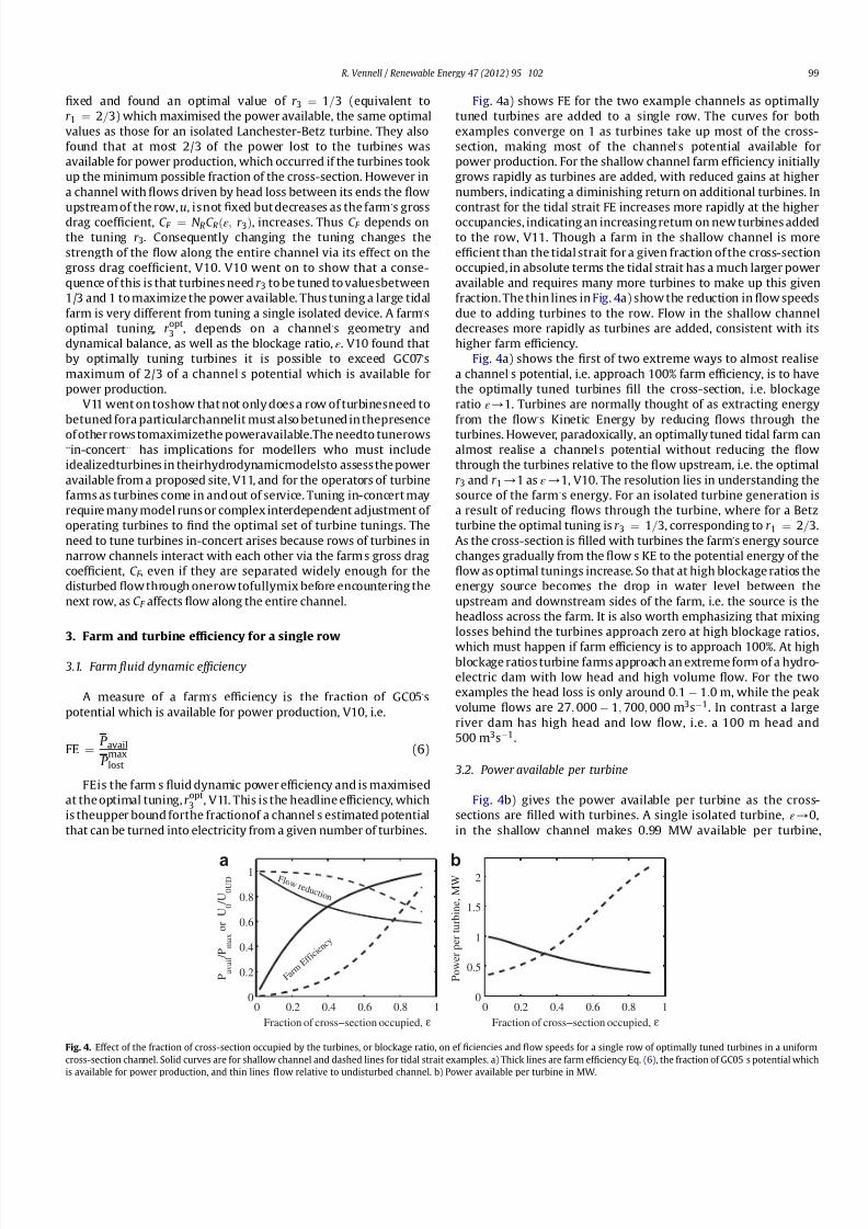
8132019 Efficiency of Tidal Turbine Farms
httpslidepdfcomreaderfullefficiency-of-tidal-turbine-farms 58
1047297xed and found an optimal value of r 3 frac14 1=3 (equivalent to
r 1 frac14 2=3) which maximised the power available the same optimal
values as those for an isolated Lanchester-Betz turbine They also
found that at most 23 of the power lost to the turbines was
available for power production which occurred if the turbines took
up the minimum possible fraction of the cross-section However in
a channel with 1047298ows driven by head loss between its ends the 1047298ow
upstream of the row u isnot 1047297xed but decreases as the farmrsquos gross
drag coef 1047297cient C F frac14 N RC Rethε r 3THORN increases Thus C F depends on
the tuning r 3 Consequently changing the tuning changes the
strength of the 1047298ow along the entire channel via its effect on the
gross drag coef 1047297cient V10 V10 went on to show that a conse-
quence of this is that turbines need r 3 to be tuned to valuesbetween
13 and 1 to maximize the power available Thus tuning a large tidal
farm is very different from tuning a single isolated device A farmrsquos
optimal tuning r opt3 depends on a channelrsquos geometry and
dynamical balance as well as the blockage ratio ε V10 found that
by optimally tuning turbines it is possible to exceed GC07rsquos
maximum of 23 of a channelrsquos potential which is available for
power production
V11 went on toshow that not only does a row of turbinesneed to
betuned fora particularchannelit must also betuned in thepresence
of other rows tomaximizethe poweravailableThe needto tunerowsldquoin-concertrdquo has implications for modellers who must include
idealizedturbines in theirhydrodynamicmodelsto assess the power
available from a proposed site V11 and for the operators of turbine
farms as turbines come in and out of service Tuning in-concert may
require many model runs or complex interdependent adjustment of
operating turbines to 1047297nd the optimal set of turbine tunings The
need to tune turbines in-concert arises because rows of turbines in
narrow channels interact with each other via the farmrsquos gross drag
coef 1047297cient C F even if they are separated widely enough for the
disturbed 1047298ow through onerow tofullymix before encountering the
next row as C F affects 1047298ow along the entire channel
3 Farm and turbine ef 1047297ciency for a single row
31 Farm 1047298uid dynamic ef 1047297ciency
A measure of a farmrsquos ef 1047297ciency is the fraction of GC05rsquos
potential which is available for power production V10 ie
FE frac14 P avail
P maxlost
(6)
FEis the farmrsquos 1047298uid dynamic power ef 1047297ciency and is maximised
at the optimal tuning r opt3 V11 This is the headline ef 1047297ciency which
is theupper bound forthe fractionof a channelrsquos estimated potential
that can be turned into electricity from a given number of turbines
Fig 4a) shows FE for the two example channels as optimally
tuned turbines are added to a single row The curves for both
examples converge on 1 as turbines take up most of the cross-
section making most of the channelrsquos potential available for
power production For the shallow channel farm ef 1047297ciency initially
grows rapidly as turbines are added with reduced gains at higher
numbers indicating a diminishing return on additional turbines In
contrast for the tidal strait FE increases more rapidly at the higher
occupancies indicating an increasing return on new turbines added
to the row V11 Though a farm in the shallow channel is more
ef 1047297cient than the tidal strait for a given fraction of the cross-section
occupied in absolute terms the tidal strait has a much larger power
available and requires many more turbines to make up this given
fraction The thin lines in Fig 4a) show the reduction in 1047298ow speeds
due to adding turbines to the row Flow in the shallow channel
decreases more rapidly as turbines are added consistent with its
higher farm ef 1047297ciency
Fig 4a) shows the 1047297rst of two extreme ways to almost realise
a channelrsquos potential ie approach 100 farm ef 1047297ciency is to have
the optimally tuned turbines 1047297ll the cross-section ie blockage
ratio ε1 Turbines are normally thought of as extracting energy
from the 1047298owrsquos Kinetic Energy by reducing 1047298ows through the
turbines However paradoxically an optimally tuned tidal farm canalmost realise a channelrsquos potential without reducing the 1047298ow
through the turbines relative to the 1047298ow upstream ie the optimal
r 3 and r 11 as ε1 V10 The resolution lies in understanding the
source of the farmrsquos energy For an isolated turbine generation is
a result of reducing 1047298ows through the turbine where for a Betz
turbine the optimal tuning is r 3 frac14 1=3 corresponding to r 1 frac14 2=3
As the cross-section is 1047297lled with turbines the farmrsquos energy source
changes gradually from the 1047298owrsquos KE to the potential energy of the
1047298ow as optimal tunings increase So that at high blockage ratios the
energy source becomes the drop in water level between the
upstream and downstream sides of the farm ie the source is the
headloss across the farm It is also worth emphasizing that mixing
losses behind the turbines approach zero at high blockage ratios
which must happen if farm ef 1047297ciency is to approach 100 At highblockage ratios turbine farms approach an extreme form of a hydro-
electric dam with low head and high volume 1047298ow For the two
examples the head loss is only around 01 10 m while the peak
volume 1047298ows are 27 000 1 700 000 m3s1 In contrast a large
river dam has high head and low 1047298ow ie a 100 m head and
500 m3s1
32 Power available per turbine
Fig 4b) gives the power available per turbine as the cross-
sections are 1047297lled with turbines A single isolated turbine ε0
in the shallow channel makes 099 MW available per turbine
0 02 04 06 08 10
02
04
06
08
1
Fraction of crossminussection occupied ε
P a v a i l P m a x
o r U 0
U 0 U Da
F a r m
E f f i
c i e n c
y
F l o w r e d u c t i o n
0 02 04 06 08 10
05
1
15
2
Fraction of crossminussection occupied ε
P o w e r p e r t u r b i n e M Wb
Fig 4 Effect of the fraction of cross-section occupied by the turbines or blockage ratio on ef 1047297ciencies and 1047298ow speeds for a single row of optimally tuned turbines in a uniform
cross-section channel Solid curves are for shallow channel and dashed lines for tidal strait examples a) Thick lines are farm ef 1047297ciency Eq (6) the fraction of GC05rsquos potential which
is available for power production and thin lines 1047298
ow relative to undisturbed channel b) Power available per turbine in MW
R Vennell Renewable Energy 47 (2012) 95e102 99
8132019 Efficiency of Tidal Turbine Farms
httpslidepdfcomreaderfullefficiency-of-tidal-turbine-farms 68
whereas only 034 MW is available in the tidal strait due to much
weaker 1047298ows However as the cross-section is 1047297lled the power
available per turbine for the shallow channel decreases while for
the tidal strait power per turbine increases So paradoxically at
higher occupancies the tidal strait delivers up to six times more per
turbine despite having much weaker 1047298ows than the shallow
channel The curves in Fig 4b) are the result of two competing
effects Firstly occupying more of the cross-section increases
a rowrsquos drag coef 1047297cient C R increases the power available Eq (5)
Secondly increasing a rows drag coef 1047297cient reduces the 1047298ow along
the channel U 0 which acts to decrease the power available in Eq
(5) The net effect differs for the two examples For the shallow
channel the more rapid reduction in 1047298ow speed as the cross-section
is 1047297lled Fig 4a) outweighs the enhanced drag coef 1047297cient leading
to reduction in the power per turbine from 099 MW to only
036 MW at high occupancy In contrast the more gradual 1047298ow
reduction in the tidal strait leads to an increasing power available
per turbine as the cross-section is 1047297lledfrom 034MW to23MW A
result is that above 35 occupancy the tidal strait delivers more per
turbine than the shallow channel despite the much weaker 1047298ows in
the strait
The differing performance of the turbines as the cross-section is
1047297lled is linked to their differing dynamical balances At higheroccupancies in the shallow channel the power lost to the turbines is
similar to that lost to background friction (this can be inferred from
(V10-A4) where C F peak is around twice the scaled background
bottom friction coef 1047297cient C D for near steady state channels ie
large l0 channels) This signi1047297cant energy loss to bottom friction
and turbine drag is associated with a more rapid decrease in 1047298ows
a diminishing return on new turbines and the decreasing power
available per turbine in Fig 4 In contrast in the tidal strait bottom
friction is almost unimportant and relatively little energy is lost to
bottom friction This gives the strait a proportionately higher
potential and an increasing return on additional turbines as they
becomemore ef 1047297cient when occupying more of the cross-section of
the ldquoductrdquo formed by the channel The energetics of channels with
turbine farms is discussed in detail in [17]
4 Ef 1047297ciency of multi-row farms
Adding capacity to a farm by adding rows of optimally tuned
turbines increases farm ef 1047297ciency as demonstrated in Fig 5a) For
the tidal strait 15 rows makes only 40 of it potential available so as
would be expected the associated 1047298ow reduction is modest In
contrast for the shallow channel 3 rows make 70 of its potential
available with a signi1047297cant associated 1047298ow reduction
Fig 5 illustrates a second extreme way to realize most of
a channelrsquos potential having a large number of rows However for
both channels there is a diminishing return on additional rows
Farm ef 1047297ciency peaks at a very large number of rows indicating an
optimal farm size However the diminishing return on new rows is
so harsh near this peak that farm size will be restricted to a much
smaller of number rows [17] V11 showed that for two similar
examples the best strategy for growing a farm of optimally tuned
turbines is the intuitive one Fill the 1047297rst row up to the maximum
permitted by navigational constraints and then add rows up to
a maximum that can be economically justi1047297ed in the light of the
diminishing returns inherent in Fig 5a)
5 Realizing the potential a trade off
The decision on turbine numbers is an economic trade off
between the income from the power made available by adding
turbines to a farm against their cost and any environmental
impacts Once the maximum permissible cross-sectional occu-
pancy has been achieved then the trade off is in the face of
a diminishing return on additional turbines Fig 5a) How this trade
off plays out depends strongly on the maximum fraction of the
channelrsquos cross-section which can be occupied in order to maintain
navigation along the channel It also strongly depends on the
dynamical balance of the undisturbed channel be it that of
a bottom friction dominated shallow channel or that of an inertia
dominated tidal strait Fig 5
This diminishing return is inherent in the upper row of plots in
Fig 6 where for both a low cross-sectional occupancy ε frac14 01 and
what may be an unrealistically high occupancy ε frac14 05 power
available increases more slowly as rows are added to an optimally
tuned farm While the ultimate choice on number of turbines
comes down to an economic and environmental cost bene1047297t
analysis which is beyond the scope of this work the plots however
do contain essential information to underpin this analysis For the
shallow channel at the high occupancy 1 row of 12 turbines makes
80 of its 9 MW potential available Fig 6a) In contrast the same
number of turbines spread across 5 rows at the lower occupancy
makes only 65 of the potential available for power productionFig 6c) shows that the power available per turbine for both occu-
pancies decreases as rows are added Fig 6e) illustrates that for
both occupancies a farm making 80 of the shallow channelrsquos
potential available will reduce 1047298ows by 30 If such a signi1047297cant
1047298ow reduction is not acceptable then at the lower occupancy
installing around 3 turbines reduces 1047298ows by only 10 while
making around 25 of its potential available
The curves for the tidal strait in Fig 6b) d) and f) are similar to
those of the shallow channel but the number of turbines involved
is much larger Almost 80 of the straitrsquos 6 GW potential can be
realized at the higher occupancy but this requires an astonishing
0 5 10 150
02
04
06
08
1
Number of Rows NR
a
Farm Efficiency
0 5 10 1504
06
08
1
Number of Rows NR
b
Flow reduction
Fig 5 Effect of adding rows to an optimally tuned farm where turbines occupy 20 of the channel rsquos cross-section ie a blockage ratio of ε frac14 02 Solid curves are for the shallow
channel and dashed lines for the tidal strait a) Farm ef 1047297
ciency Eq (6) b) Velocity relative to undisturbed velocity
R Vennell Renewable Energy 47 (2012) 95e102100
8132019 Efficiency of Tidal Turbine Farms
httpslidepdfcomreaderfullefficiency-of-tidal-turbine-farms 78
16000 turbines spread over 13 rows At the lower occupancy
a more affordable 5000 turbines would make 30 of the strait rsquos
potential available while reducing 1047298ows by 7
6 Discussion
The principle aim of this paper was to show how many turbines
are required to realize a given fraction of a channel rsquos potential in
order to improve understanding of how power production scales
with farm size The models in V10 and V11 which build on those of
GC05 and GC07 provide the 1047297rst physically coherent way of con-
necting the number of turbines in a farm with the maximum power
available for electricity production The models do not require the
use of arbitrary loading or safety factors applied to account for
unknown effects The models are however simple They use an
extended form of classic turbine theory and they only apply to the
cross-sectional average velocities thusdo not account for the effects
of any variation of 1047298ow across the channel or with depth They also
do not allow for any effect of the turbulence shed by a row on the
ef 1047297
ciency of downstream rows They do not allow for minimum
turbine operating 1047298ows or for loss due to their electro-mechanical
ef 1047297ciency or transmission and conversion losses Thus there is
muchworktobedonetore1047297ne and extend the modelsHowever the
models do illuminate signi1047297cant aspects of developing large tidal
turbine farms Most of these are a result of power extraction
reducing the 1047298ows along the entire narrow channel via the farmrsquos
gross dragcoef 1047297cient C F They include thenecessity totune turbines
for the particular channel and in relation to each other which will
result in signi1047297cant computational cost to those modelling turbine
farms and will require on going optimization of turbine tuning in
large operational farms as turbines come in and out of service They
also include how farms have increasing or diminishing returns on
turbines added to thecross-section dependingon the importance of
bottom friction and how there is always a diminishing return on
additional rows aspects which are fundamental to understanding
the economics of farm development
The turbine numbers given by the simple models should be
viewed as estimates of the magnitude of the numbers required
rather than precise estimates These magnitudes are useful in
understanding how realistic it is to realize a signi1047297
cant fraction of
0 10 20 30 400
02
04
06
08
1
1
3
5
101
3
P o w e r P
m a x
Number of Turbines
aShallow Channel
0 5 10 150
02
04
06
08
1
1
5
10
20
50
1
5
10
P o w e r P
m a x
Thousands of Turbines
bTidal Strait
0 10 20 30 400
02
04
06
08
1
12
P o w
e r P e r T u r b i n e M W
Number of Turbines
c
0 5 100
02
04
06
08
1
12
P o w
e r P e r T u r b i n e M W
Thousands of Turbines
d
06 07 08 09 10
02
04
06
08
1
5
10
15
2515
25
P o w e r P
m a x
Flow Reduction
e
06 07 08 09 10
02
04
06
08
1
10002000
5000
10000
15000
2000
5000
10000
15000
P o w e r P
m a x
Flow Reduction
f
Fig 6 Effect of the number of optimally tuned turbines on power available and 1047298ow reduction for the two example channels based on a 400 m 2 blade area Solid curves are for
ε frac14 01 and dashed lines for ε frac14 05 a) and b) Farm ef 1047297ciency versus number of turbines labelled dots give number of rows in the farm c) and d) Power available per turbine in
MW e) and f) Farm ef 1047297ciency verses 1047298ow reduction Labelled dots give the number of turbines in farm
R Vennell Renewable Energy 47 (2012) 95e102 101
8132019 Efficiency of Tidal Turbine Farms
httpslidepdfcomreaderfullefficiency-of-tidal-turbine-farms 88
a channelrsquos potential For the shallow channel around eight 400 m2
turbines corresponding to three rows with ε frac14 01 makes half of
its potential available and 13 corresponding to one row with
ε frac14 05 makes 80 available Table 1 The given values for the
power available per turbine are also useful in understanding
economic feasibility For blockage ratios of ε frac14 01 and 05 each
turbine makes around 06 MW available The detailed economics
and environmental costs are beyond the scope of this work
however making an average of 06 MWavailable over the tidal cycle
when existing turbines are producing around 1 MW at steady1047298ows
around2 m s1 maybe a reasonable return Thus it appears possible
to make a signi1047297cant fraction of the shallow channelrsquos potential
available using 5e10 turbines with a blade area similar to that of
the largest currently operating tidal turbine spread amongst 1e3
rows which occupy less than 50 of the cross-section
In contrast to make 50 of the tidal straitrsquos 6 GW potential
available takes 10000 turbines at 10 blockage This high number
is a result of the weaker 1047298ows in the tidal strait which yield only
027 MW per turbine However unlike the tidal shallow channel
the output per turbine rises as more of the strait rsquos cross-section is
occupied So that at 50 blockage only 5000 turbines are required
to make 50 of its potentialavailable at a much higher 061MW per
turbine similar to that for the shallow channel Tidal straits haveboth a much larger potential in absolute terms and in proportion to
their size due to relatively low energy losses to bottom friction
This is seen in their having six times the potential per turbinewhen
turbines 1047297ll the cross-section in a single row Table 1 However tidal
straits typically have weaker cross-sectionally averaged 1047298ows than
shallow tidal channels Thus at low blockage ratios a very large
number of rows are required to make a signi1047297cant fraction avail-
able If higher blockage ratios are permitted then the enhanced
ef 1047297ciency of turbines in tidal straits seen in Fig 4 boosts the output
per turbine and reduces the total number of turbines required [17]
uses the channelrsquos energy balance to explain why and when tidal
straits have an increasing return on turbines added to the cross-
section and why shallow channels have a diminishing return
7 Conclusions
Critical questions in developing a farm are what fraction of
a channelrsquos potential is available for power production from a given
number of turbines as a farm scales up from a single turbine into
a large farm The V10 thorn V11 works provide the 1047297rst physically
coherent way to connect the number of turbines in a farm to both
the maximum power available for electricity production and to the
degree of 1047298ow reduction which is a consequence of power
extraction Though simple they illuminate several important
aspects of developing large farms which have implications for both
the economics and environmental impact of farms Such as the
necessity of tuning turbines in large farms for the particular
channel how much of the cross-section they occupy and the
number of rows as well as how to best arrange and con1047297gure the
turbines For example to maximize farm ef 1047297ciency the 1047297rst row
turbines should be 1047297lled up to the maximum permitted by navi-
gational constraints before adding new rows Also while farm
ef 1047297ciency always increases as optimally tuned turbines are added
once the cross-sectional occupancy limit is attained the power
available per turbine decreases as rows are added Thus increasing
power production by increasing the farmrsquos installed capacity faces
a diminishing return on additional rows This development strategy
may alter when more realistic models are developed which allow
for variation of 1047298ow across the channel and with depth However
the decision on turbine numbers will remain an economic trade off
between the power produced and installation maintenance and
environmental costs How this trade off plays out depends strongly
on the maximum fraction of the channelrsquos cross-section which can
be occupied and the dynamical balance of the undisturbed channel
The examples demonstrate that it may be possible with existing
technology to realize much of the MW potential of shallow tidal
channels The GW potential of tidal straits is both larger in absolute
terms and also proportionately larger than that of shallow chan-
nels due to relatively low energy losses to bottom friction At low
cross-sectional occupancies the typically lower 1047298ows of the strait
result in both a low return per turbine and a very large number of
turbines being required to realize a signi1047297cant fraction of their
proportionately higher potential Thus unless a large fraction of the
straitrsquos cross-section can be occupied to take advantage of a higher
output per turbine it will be dif 1047297cult to realize a substantial frac-
tion of the GW potential of tidal straits until larger turbines are
developed which are able operate economically in low 1047298ows
References
[1] Garrett C Cummins P The power potential of tidal currents in channels
Proceedings of the Royal Society A 20054612563e
72[2] Blunden LS Bahaj AS Tidal energy resource assessment for tidal stream
generators Proceedings of the Institution of Mechanical Engineers Part A Journal of Power and Energy 2007221(10)137e46 doi10124309576509JPE332
[3] Blanch1047297eld J Garrett C Rowe A Wild P Tidal stream power resourceassessment for Masset Sound Haida Gwaii Proceedings of the Institution of Mechanical Engineers Part A Journal of Power and Energy 2008222(5)485e92
[4] Neill SP Litt EJ Couch SJ Davies AG The impact of tidal stream turbines onlarge-scale sediment dynamics Renewable Energy 200934(12)2803e12doi101016jrenene200906015
[5] Garrett C Cummins P Limits to tidal current power Renewable Energy 2008332485e90
[6] Garrett C Cummins P Tuning turbines in a tidal channel Journal of FluidMechanics 2010663253e67 doi101017S0022112010003502
[7] Vennell R Tuning tidal turbines in concert to maximise farm ef 1047297ciency Journal of Fluid Mechanics 2011671587e604
[8] Garrett C Cummins P The ef 1047297
ciency of a turbine in a tidal channel Journal of Fluid Mechanics 2007588243e51[9] Blanch1047297eld J Garrett C Wild P Rowe A The extractable power from a channel
linking a bay to the open ocean Proceedings of the Institution of MechanicalEngineers Part A Journal of Power and Energy 2008222(3)289e97
[10] Vennell R Estimating the power potential of tidal currents and the impact of power extraction on 1047298ow speeds Renewable Energy 2011363558e65 doi101016jrenene201105011
[11] Arbic B Garrett C A coupled oscillator model of shelf and ocean tidesContinental Shelf Research 201030(6)564e74
[12] Vennell R Oscillating barotropic currents along short channels Journal of Physical Oceanography 199828(8)1561e9
[13] Vennell R Observations of the phase of tidal currents along a strait Journal of Physical Oceanography 199828(8)1570e7
[14] Byden IG Grinsted T Melville GT Assessing the potential of a simple tidalchannel to deliver useful energy Journal of Applied Ocean Research 200426198e204 doi101016japor200504001
[15] Vennell R ADCP measurements of tidal phase and amplitude in Cook StraitNew Zealand Continental Shelf Research 199414353e64
[16] Douglas C Harrison G Chick J Life cycle assessment of the Seagen marinecurrent turbine Proceedings of the Institution of Mechanical Engineers Part M
Journal of Engineering for the Maritime Environment 2008222(1)1e12 doi10124314750902JEME94
[17] Vennell R The energetics of large tidal turbine arrays Renewable Energyin press
[18] Vennell R ADCP measurements of momentum balance and dynamic topog-raphy in a constricted tidal channel Journal of Physical Oceanography 200636(2)177e88
[19] Corten G Heat generation by a wind turbine Vol In 14th IEA symposium onthe aerodynamics of wind turbines 2000 p 7 ECN report ECN-RX-01-001
[20] Lanchester FW A contribution to the theory of propulsion and the screwpropeller Transactions of the Institution of Naval Architects 1915LVII98e116
[21] Betz A Das Maximum der theoretisch moumlglichen Ausnutzung des Windesdurch Windmotoren Gesamte Turbinenwesen 192017307e9
R Vennell Renewable Energy 47 (2012) 95e102102
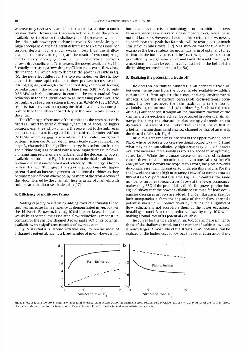
8132019 Efficiency of Tidal Turbine Farms
httpslidepdfcomreaderfullefficiency-of-tidal-turbine-farms 68
whereas only 034 MW is available in the tidal strait due to much
weaker 1047298ows However as the cross-section is 1047297lled the power
available per turbine for the shallow channel decreases while for
the tidal strait power per turbine increases So paradoxically at
higher occupancies the tidal strait delivers up to six times more per
turbine despite having much weaker 1047298ows than the shallow
channel The curves in Fig 4b) are the result of two competing
effects Firstly occupying more of the cross-section increases
a rowrsquos drag coef 1047297cient C R increases the power available Eq (5)
Secondly increasing a rows drag coef 1047297cient reduces the 1047298ow along
the channel U 0 which acts to decrease the power available in Eq
(5) The net effect differs for the two examples For the shallow
channel the more rapid reduction in 1047298ow speed as the cross-section
is 1047297lled Fig 4a) outweighs the enhanced drag coef 1047297cient leading
to reduction in the power per turbine from 099 MW to only
036 MW at high occupancy In contrast the more gradual 1047298ow
reduction in the tidal strait leads to an increasing power available
per turbine as the cross-section is 1047297lledfrom 034MW to23MW A
result is that above 35 occupancy the tidal strait delivers more per
turbine than the shallow channel despite the much weaker 1047298ows in
the strait
The differing performance of the turbines as the cross-section is
1047297lled is linked to their differing dynamical balances At higheroccupancies in the shallow channel the power lost to the turbines is
similar to that lost to background friction (this can be inferred from
(V10-A4) where C F peak is around twice the scaled background
bottom friction coef 1047297cient C D for near steady state channels ie
large l0 channels) This signi1047297cant energy loss to bottom friction
and turbine drag is associated with a more rapid decrease in 1047298ows
a diminishing return on new turbines and the decreasing power
available per turbine in Fig 4 In contrast in the tidal strait bottom
friction is almost unimportant and relatively little energy is lost to
bottom friction This gives the strait a proportionately higher
potential and an increasing return on additional turbines as they
becomemore ef 1047297cient when occupying more of the cross-section of
the ldquoductrdquo formed by the channel The energetics of channels with
turbine farms is discussed in detail in [17]
4 Ef 1047297ciency of multi-row farms
Adding capacity to a farm by adding rows of optimally tuned
turbines increases farm ef 1047297ciency as demonstrated in Fig 5a) For
the tidal strait 15 rows makes only 40 of it potential available so as
would be expected the associated 1047298ow reduction is modest In
contrast for the shallow channel 3 rows make 70 of its potential
available with a signi1047297cant associated 1047298ow reduction
Fig 5 illustrates a second extreme way to realize most of
a channelrsquos potential having a large number of rows However for
both channels there is a diminishing return on additional rows
Farm ef 1047297ciency peaks at a very large number of rows indicating an
optimal farm size However the diminishing return on new rows is
so harsh near this peak that farm size will be restricted to a much
smaller of number rows [17] V11 showed that for two similar
examples the best strategy for growing a farm of optimally tuned
turbines is the intuitive one Fill the 1047297rst row up to the maximum
permitted by navigational constraints and then add rows up to
a maximum that can be economically justi1047297ed in the light of the
diminishing returns inherent in Fig 5a)
5 Realizing the potential a trade off
The decision on turbine numbers is an economic trade off
between the income from the power made available by adding
turbines to a farm against their cost and any environmental
impacts Once the maximum permissible cross-sectional occu-
pancy has been achieved then the trade off is in the face of
a diminishing return on additional turbines Fig 5a) How this trade
off plays out depends strongly on the maximum fraction of the
channelrsquos cross-section which can be occupied in order to maintain
navigation along the channel It also strongly depends on the
dynamical balance of the undisturbed channel be it that of
a bottom friction dominated shallow channel or that of an inertia
dominated tidal strait Fig 5
This diminishing return is inherent in the upper row of plots in
Fig 6 where for both a low cross-sectional occupancy ε frac14 01 and
what may be an unrealistically high occupancy ε frac14 05 power
available increases more slowly as rows are added to an optimally
tuned farm While the ultimate choice on number of turbines
comes down to an economic and environmental cost bene1047297t
analysis which is beyond the scope of this work the plots however
do contain essential information to underpin this analysis For the
shallow channel at the high occupancy 1 row of 12 turbines makes
80 of its 9 MW potential available Fig 6a) In contrast the same
number of turbines spread across 5 rows at the lower occupancy
makes only 65 of the potential available for power productionFig 6c) shows that the power available per turbine for both occu-
pancies decreases as rows are added Fig 6e) illustrates that for
both occupancies a farm making 80 of the shallow channelrsquos
potential available will reduce 1047298ows by 30 If such a signi1047297cant
1047298ow reduction is not acceptable then at the lower occupancy
installing around 3 turbines reduces 1047298ows by only 10 while
making around 25 of its potential available
The curves for the tidal strait in Fig 6b) d) and f) are similar to
those of the shallow channel but the number of turbines involved
is much larger Almost 80 of the straitrsquos 6 GW potential can be
realized at the higher occupancy but this requires an astonishing
0 5 10 150
02
04
06
08
1
Number of Rows NR
a
Farm Efficiency
0 5 10 1504
06
08
1
Number of Rows NR
b
Flow reduction
Fig 5 Effect of adding rows to an optimally tuned farm where turbines occupy 20 of the channel rsquos cross-section ie a blockage ratio of ε frac14 02 Solid curves are for the shallow
channel and dashed lines for the tidal strait a) Farm ef 1047297
ciency Eq (6) b) Velocity relative to undisturbed velocity
R Vennell Renewable Energy 47 (2012) 95e102100
8132019 Efficiency of Tidal Turbine Farms
httpslidepdfcomreaderfullefficiency-of-tidal-turbine-farms 78
16000 turbines spread over 13 rows At the lower occupancy
a more affordable 5000 turbines would make 30 of the strait rsquos
potential available while reducing 1047298ows by 7
6 Discussion
The principle aim of this paper was to show how many turbines
are required to realize a given fraction of a channel rsquos potential in
order to improve understanding of how power production scales
with farm size The models in V10 and V11 which build on those of
GC05 and GC07 provide the 1047297rst physically coherent way of con-
necting the number of turbines in a farm with the maximum power
available for electricity production The models do not require the
use of arbitrary loading or safety factors applied to account for
unknown effects The models are however simple They use an
extended form of classic turbine theory and they only apply to the
cross-sectional average velocities thusdo not account for the effects
of any variation of 1047298ow across the channel or with depth They also
do not allow for any effect of the turbulence shed by a row on the
ef 1047297
ciency of downstream rows They do not allow for minimum
turbine operating 1047298ows or for loss due to their electro-mechanical
ef 1047297ciency or transmission and conversion losses Thus there is
muchworktobedonetore1047297ne and extend the modelsHowever the
models do illuminate signi1047297cant aspects of developing large tidal
turbine farms Most of these are a result of power extraction
reducing the 1047298ows along the entire narrow channel via the farmrsquos
gross dragcoef 1047297cient C F They include thenecessity totune turbines
for the particular channel and in relation to each other which will
result in signi1047297cant computational cost to those modelling turbine
farms and will require on going optimization of turbine tuning in
large operational farms as turbines come in and out of service They
also include how farms have increasing or diminishing returns on
turbines added to thecross-section dependingon the importance of
bottom friction and how there is always a diminishing return on
additional rows aspects which are fundamental to understanding
the economics of farm development
The turbine numbers given by the simple models should be
viewed as estimates of the magnitude of the numbers required
rather than precise estimates These magnitudes are useful in
understanding how realistic it is to realize a signi1047297
cant fraction of
0 10 20 30 400
02
04
06
08
1
1
3
5
101
3
P o w e r P
m a x
Number of Turbines
aShallow Channel
0 5 10 150
02
04
06
08
1
1
5
10
20
50
1
5
10
P o w e r P
m a x
Thousands of Turbines
bTidal Strait
0 10 20 30 400
02
04
06
08
1
12
P o w
e r P e r T u r b i n e M W
Number of Turbines
c
0 5 100
02
04
06
08
1
12
P o w
e r P e r T u r b i n e M W
Thousands of Turbines
d
06 07 08 09 10
02
04
06
08
1
5
10
15
2515
25
P o w e r P
m a x
Flow Reduction
e
06 07 08 09 10
02
04
06
08
1
10002000
5000
10000
15000
2000
5000
10000
15000
P o w e r P
m a x
Flow Reduction
f
Fig 6 Effect of the number of optimally tuned turbines on power available and 1047298ow reduction for the two example channels based on a 400 m 2 blade area Solid curves are for
ε frac14 01 and dashed lines for ε frac14 05 a) and b) Farm ef 1047297ciency versus number of turbines labelled dots give number of rows in the farm c) and d) Power available per turbine in
MW e) and f) Farm ef 1047297ciency verses 1047298ow reduction Labelled dots give the number of turbines in farm
R Vennell Renewable Energy 47 (2012) 95e102 101
8132019 Efficiency of Tidal Turbine Farms
httpslidepdfcomreaderfullefficiency-of-tidal-turbine-farms 88
a channelrsquos potential For the shallow channel around eight 400 m2
turbines corresponding to three rows with ε frac14 01 makes half of
its potential available and 13 corresponding to one row with
ε frac14 05 makes 80 available Table 1 The given values for the
power available per turbine are also useful in understanding
economic feasibility For blockage ratios of ε frac14 01 and 05 each
turbine makes around 06 MW available The detailed economics
and environmental costs are beyond the scope of this work
however making an average of 06 MWavailable over the tidal cycle
when existing turbines are producing around 1 MW at steady1047298ows
around2 m s1 maybe a reasonable return Thus it appears possible
to make a signi1047297cant fraction of the shallow channelrsquos potential
available using 5e10 turbines with a blade area similar to that of
the largest currently operating tidal turbine spread amongst 1e3
rows which occupy less than 50 of the cross-section
In contrast to make 50 of the tidal straitrsquos 6 GW potential
available takes 10000 turbines at 10 blockage This high number
is a result of the weaker 1047298ows in the tidal strait which yield only
027 MW per turbine However unlike the tidal shallow channel
the output per turbine rises as more of the strait rsquos cross-section is
occupied So that at 50 blockage only 5000 turbines are required
to make 50 of its potentialavailable at a much higher 061MW per
turbine similar to that for the shallow channel Tidal straits haveboth a much larger potential in absolute terms and in proportion to
their size due to relatively low energy losses to bottom friction
This is seen in their having six times the potential per turbinewhen
turbines 1047297ll the cross-section in a single row Table 1 However tidal
straits typically have weaker cross-sectionally averaged 1047298ows than
shallow tidal channels Thus at low blockage ratios a very large
number of rows are required to make a signi1047297cant fraction avail-
able If higher blockage ratios are permitted then the enhanced
ef 1047297ciency of turbines in tidal straits seen in Fig 4 boosts the output
per turbine and reduces the total number of turbines required [17]
uses the channelrsquos energy balance to explain why and when tidal
straits have an increasing return on turbines added to the cross-
section and why shallow channels have a diminishing return
7 Conclusions
Critical questions in developing a farm are what fraction of
a channelrsquos potential is available for power production from a given
number of turbines as a farm scales up from a single turbine into
a large farm The V10 thorn V11 works provide the 1047297rst physically
coherent way to connect the number of turbines in a farm to both
the maximum power available for electricity production and to the
degree of 1047298ow reduction which is a consequence of power
extraction Though simple they illuminate several important
aspects of developing large farms which have implications for both
the economics and environmental impact of farms Such as the
necessity of tuning turbines in large farms for the particular
channel how much of the cross-section they occupy and the
number of rows as well as how to best arrange and con1047297gure the
turbines For example to maximize farm ef 1047297ciency the 1047297rst row
turbines should be 1047297lled up to the maximum permitted by navi-
gational constraints before adding new rows Also while farm
ef 1047297ciency always increases as optimally tuned turbines are added
once the cross-sectional occupancy limit is attained the power
available per turbine decreases as rows are added Thus increasing
power production by increasing the farmrsquos installed capacity faces
a diminishing return on additional rows This development strategy
may alter when more realistic models are developed which allow
for variation of 1047298ow across the channel and with depth However
the decision on turbine numbers will remain an economic trade off
between the power produced and installation maintenance and
environmental costs How this trade off plays out depends strongly
on the maximum fraction of the channelrsquos cross-section which can
be occupied and the dynamical balance of the undisturbed channel
The examples demonstrate that it may be possible with existing
technology to realize much of the MW potential of shallow tidal
channels The GW potential of tidal straits is both larger in absolute
terms and also proportionately larger than that of shallow chan-
nels due to relatively low energy losses to bottom friction At low
cross-sectional occupancies the typically lower 1047298ows of the strait
result in both a low return per turbine and a very large number of
turbines being required to realize a signi1047297cant fraction of their
proportionately higher potential Thus unless a large fraction of the
straitrsquos cross-section can be occupied to take advantage of a higher
output per turbine it will be dif 1047297cult to realize a substantial frac-
tion of the GW potential of tidal straits until larger turbines are
developed which are able operate economically in low 1047298ows
References
[1] Garrett C Cummins P The power potential of tidal currents in channels
Proceedings of the Royal Society A 20054612563e
72[2] Blunden LS Bahaj AS Tidal energy resource assessment for tidal stream
generators Proceedings of the Institution of Mechanical Engineers Part A Journal of Power and Energy 2007221(10)137e46 doi10124309576509JPE332
[3] Blanch1047297eld J Garrett C Rowe A Wild P Tidal stream power resourceassessment for Masset Sound Haida Gwaii Proceedings of the Institution of Mechanical Engineers Part A Journal of Power and Energy 2008222(5)485e92
[4] Neill SP Litt EJ Couch SJ Davies AG The impact of tidal stream turbines onlarge-scale sediment dynamics Renewable Energy 200934(12)2803e12doi101016jrenene200906015
[5] Garrett C Cummins P Limits to tidal current power Renewable Energy 2008332485e90
[6] Garrett C Cummins P Tuning turbines in a tidal channel Journal of FluidMechanics 2010663253e67 doi101017S0022112010003502
[7] Vennell R Tuning tidal turbines in concert to maximise farm ef 1047297ciency Journal of Fluid Mechanics 2011671587e604
[8] Garrett C Cummins P The ef 1047297
ciency of a turbine in a tidal channel Journal of Fluid Mechanics 2007588243e51[9] Blanch1047297eld J Garrett C Wild P Rowe A The extractable power from a channel
linking a bay to the open ocean Proceedings of the Institution of MechanicalEngineers Part A Journal of Power and Energy 2008222(3)289e97
[10] Vennell R Estimating the power potential of tidal currents and the impact of power extraction on 1047298ow speeds Renewable Energy 2011363558e65 doi101016jrenene201105011
[11] Arbic B Garrett C A coupled oscillator model of shelf and ocean tidesContinental Shelf Research 201030(6)564e74
[12] Vennell R Oscillating barotropic currents along short channels Journal of Physical Oceanography 199828(8)1561e9
[13] Vennell R Observations of the phase of tidal currents along a strait Journal of Physical Oceanography 199828(8)1570e7
[14] Byden IG Grinsted T Melville GT Assessing the potential of a simple tidalchannel to deliver useful energy Journal of Applied Ocean Research 200426198e204 doi101016japor200504001
[15] Vennell R ADCP measurements of tidal phase and amplitude in Cook StraitNew Zealand Continental Shelf Research 199414353e64
[16] Douglas C Harrison G Chick J Life cycle assessment of the Seagen marinecurrent turbine Proceedings of the Institution of Mechanical Engineers Part M
Journal of Engineering for the Maritime Environment 2008222(1)1e12 doi10124314750902JEME94
[17] Vennell R The energetics of large tidal turbine arrays Renewable Energyin press
[18] Vennell R ADCP measurements of momentum balance and dynamic topog-raphy in a constricted tidal channel Journal of Physical Oceanography 200636(2)177e88
[19] Corten G Heat generation by a wind turbine Vol In 14th IEA symposium onthe aerodynamics of wind turbines 2000 p 7 ECN report ECN-RX-01-001
[20] Lanchester FW A contribution to the theory of propulsion and the screwpropeller Transactions of the Institution of Naval Architects 1915LVII98e116
[21] Betz A Das Maximum der theoretisch moumlglichen Ausnutzung des Windesdurch Windmotoren Gesamte Turbinenwesen 192017307e9
R Vennell Renewable Energy 47 (2012) 95e102102
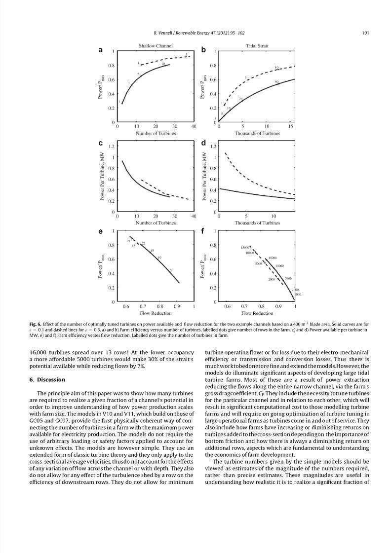
8132019 Efficiency of Tidal Turbine Farms
httpslidepdfcomreaderfullefficiency-of-tidal-turbine-farms 78
16000 turbines spread over 13 rows At the lower occupancy
a more affordable 5000 turbines would make 30 of the strait rsquos
potential available while reducing 1047298ows by 7
6 Discussion
The principle aim of this paper was to show how many turbines
are required to realize a given fraction of a channel rsquos potential in
order to improve understanding of how power production scales
with farm size The models in V10 and V11 which build on those of
GC05 and GC07 provide the 1047297rst physically coherent way of con-
necting the number of turbines in a farm with the maximum power
available for electricity production The models do not require the
use of arbitrary loading or safety factors applied to account for
unknown effects The models are however simple They use an
extended form of classic turbine theory and they only apply to the
cross-sectional average velocities thusdo not account for the effects
of any variation of 1047298ow across the channel or with depth They also
do not allow for any effect of the turbulence shed by a row on the
ef 1047297
ciency of downstream rows They do not allow for minimum
turbine operating 1047298ows or for loss due to their electro-mechanical
ef 1047297ciency or transmission and conversion losses Thus there is
muchworktobedonetore1047297ne and extend the modelsHowever the
models do illuminate signi1047297cant aspects of developing large tidal
turbine farms Most of these are a result of power extraction
reducing the 1047298ows along the entire narrow channel via the farmrsquos
gross dragcoef 1047297cient C F They include thenecessity totune turbines
for the particular channel and in relation to each other which will
result in signi1047297cant computational cost to those modelling turbine
farms and will require on going optimization of turbine tuning in
large operational farms as turbines come in and out of service They
also include how farms have increasing or diminishing returns on
turbines added to thecross-section dependingon the importance of
bottom friction and how there is always a diminishing return on
additional rows aspects which are fundamental to understanding
the economics of farm development
The turbine numbers given by the simple models should be
viewed as estimates of the magnitude of the numbers required
rather than precise estimates These magnitudes are useful in
understanding how realistic it is to realize a signi1047297
cant fraction of
0 10 20 30 400
02
04
06
08
1
1
3
5
101
3
P o w e r P
m a x
Number of Turbines
aShallow Channel
0 5 10 150
02
04
06
08
1
1
5
10
20
50
1
5
10
P o w e r P
m a x
Thousands of Turbines
bTidal Strait
0 10 20 30 400
02
04
06
08
1
12
P o w
e r P e r T u r b i n e M W
Number of Turbines
c
0 5 100
02
04
06
08
1
12
P o w
e r P e r T u r b i n e M W
Thousands of Turbines
d
06 07 08 09 10
02
04
06
08
1
5
10
15
2515
25
P o w e r P
m a x
Flow Reduction
e
06 07 08 09 10
02
04
06
08
1
10002000
5000
10000
15000
2000
5000
10000
15000
P o w e r P
m a x
Flow Reduction
f
Fig 6 Effect of the number of optimally tuned turbines on power available and 1047298ow reduction for the two example channels based on a 400 m 2 blade area Solid curves are for
ε frac14 01 and dashed lines for ε frac14 05 a) and b) Farm ef 1047297ciency versus number of turbines labelled dots give number of rows in the farm c) and d) Power available per turbine in
MW e) and f) Farm ef 1047297ciency verses 1047298ow reduction Labelled dots give the number of turbines in farm
R Vennell Renewable Energy 47 (2012) 95e102 101
8132019 Efficiency of Tidal Turbine Farms
httpslidepdfcomreaderfullefficiency-of-tidal-turbine-farms 88
a channelrsquos potential For the shallow channel around eight 400 m2
turbines corresponding to three rows with ε frac14 01 makes half of
its potential available and 13 corresponding to one row with
ε frac14 05 makes 80 available Table 1 The given values for the
power available per turbine are also useful in understanding
economic feasibility For blockage ratios of ε frac14 01 and 05 each
turbine makes around 06 MW available The detailed economics
and environmental costs are beyond the scope of this work
however making an average of 06 MWavailable over the tidal cycle
when existing turbines are producing around 1 MW at steady1047298ows
around2 m s1 maybe a reasonable return Thus it appears possible
to make a signi1047297cant fraction of the shallow channelrsquos potential
available using 5e10 turbines with a blade area similar to that of
the largest currently operating tidal turbine spread amongst 1e3
rows which occupy less than 50 of the cross-section
In contrast to make 50 of the tidal straitrsquos 6 GW potential
available takes 10000 turbines at 10 blockage This high number
is a result of the weaker 1047298ows in the tidal strait which yield only
027 MW per turbine However unlike the tidal shallow channel
the output per turbine rises as more of the strait rsquos cross-section is
occupied So that at 50 blockage only 5000 turbines are required
to make 50 of its potentialavailable at a much higher 061MW per
turbine similar to that for the shallow channel Tidal straits haveboth a much larger potential in absolute terms and in proportion to
their size due to relatively low energy losses to bottom friction
This is seen in their having six times the potential per turbinewhen
turbines 1047297ll the cross-section in a single row Table 1 However tidal
straits typically have weaker cross-sectionally averaged 1047298ows than
shallow tidal channels Thus at low blockage ratios a very large
number of rows are required to make a signi1047297cant fraction avail-
able If higher blockage ratios are permitted then the enhanced
ef 1047297ciency of turbines in tidal straits seen in Fig 4 boosts the output
per turbine and reduces the total number of turbines required [17]
uses the channelrsquos energy balance to explain why and when tidal
straits have an increasing return on turbines added to the cross-
section and why shallow channels have a diminishing return
7 Conclusions
Critical questions in developing a farm are what fraction of
a channelrsquos potential is available for power production from a given
number of turbines as a farm scales up from a single turbine into
a large farm The V10 thorn V11 works provide the 1047297rst physically
coherent way to connect the number of turbines in a farm to both
the maximum power available for electricity production and to the
degree of 1047298ow reduction which is a consequence of power
extraction Though simple they illuminate several important
aspects of developing large farms which have implications for both
the economics and environmental impact of farms Such as the
necessity of tuning turbines in large farms for the particular
channel how much of the cross-section they occupy and the
number of rows as well as how to best arrange and con1047297gure the
turbines For example to maximize farm ef 1047297ciency the 1047297rst row
turbines should be 1047297lled up to the maximum permitted by navi-
gational constraints before adding new rows Also while farm
ef 1047297ciency always increases as optimally tuned turbines are added
once the cross-sectional occupancy limit is attained the power
available per turbine decreases as rows are added Thus increasing
power production by increasing the farmrsquos installed capacity faces
a diminishing return on additional rows This development strategy
may alter when more realistic models are developed which allow
for variation of 1047298ow across the channel and with depth However
the decision on turbine numbers will remain an economic trade off
between the power produced and installation maintenance and
environmental costs How this trade off plays out depends strongly
on the maximum fraction of the channelrsquos cross-section which can
be occupied and the dynamical balance of the undisturbed channel
The examples demonstrate that it may be possible with existing
technology to realize much of the MW potential of shallow tidal
channels The GW potential of tidal straits is both larger in absolute
terms and also proportionately larger than that of shallow chan-
nels due to relatively low energy losses to bottom friction At low
cross-sectional occupancies the typically lower 1047298ows of the strait
result in both a low return per turbine and a very large number of
turbines being required to realize a signi1047297cant fraction of their
proportionately higher potential Thus unless a large fraction of the
straitrsquos cross-section can be occupied to take advantage of a higher
output per turbine it will be dif 1047297cult to realize a substantial frac-
tion of the GW potential of tidal straits until larger turbines are
developed which are able operate economically in low 1047298ows
References
[1] Garrett C Cummins P The power potential of tidal currents in channels
Proceedings of the Royal Society A 20054612563e
72[2] Blunden LS Bahaj AS Tidal energy resource assessment for tidal stream
generators Proceedings of the Institution of Mechanical Engineers Part A Journal of Power and Energy 2007221(10)137e46 doi10124309576509JPE332
[3] Blanch1047297eld J Garrett C Rowe A Wild P Tidal stream power resourceassessment for Masset Sound Haida Gwaii Proceedings of the Institution of Mechanical Engineers Part A Journal of Power and Energy 2008222(5)485e92
[4] Neill SP Litt EJ Couch SJ Davies AG The impact of tidal stream turbines onlarge-scale sediment dynamics Renewable Energy 200934(12)2803e12doi101016jrenene200906015
[5] Garrett C Cummins P Limits to tidal current power Renewable Energy 2008332485e90
[6] Garrett C Cummins P Tuning turbines in a tidal channel Journal of FluidMechanics 2010663253e67 doi101017S0022112010003502
[7] Vennell R Tuning tidal turbines in concert to maximise farm ef 1047297ciency Journal of Fluid Mechanics 2011671587e604
[8] Garrett C Cummins P The ef 1047297
ciency of a turbine in a tidal channel Journal of Fluid Mechanics 2007588243e51[9] Blanch1047297eld J Garrett C Wild P Rowe A The extractable power from a channel
linking a bay to the open ocean Proceedings of the Institution of MechanicalEngineers Part A Journal of Power and Energy 2008222(3)289e97
[10] Vennell R Estimating the power potential of tidal currents and the impact of power extraction on 1047298ow speeds Renewable Energy 2011363558e65 doi101016jrenene201105011
[11] Arbic B Garrett C A coupled oscillator model of shelf and ocean tidesContinental Shelf Research 201030(6)564e74
[12] Vennell R Oscillating barotropic currents along short channels Journal of Physical Oceanography 199828(8)1561e9
[13] Vennell R Observations of the phase of tidal currents along a strait Journal of Physical Oceanography 199828(8)1570e7
[14] Byden IG Grinsted T Melville GT Assessing the potential of a simple tidalchannel to deliver useful energy Journal of Applied Ocean Research 200426198e204 doi101016japor200504001
[15] Vennell R ADCP measurements of tidal phase and amplitude in Cook StraitNew Zealand Continental Shelf Research 199414353e64
[16] Douglas C Harrison G Chick J Life cycle assessment of the Seagen marinecurrent turbine Proceedings of the Institution of Mechanical Engineers Part M
Journal of Engineering for the Maritime Environment 2008222(1)1e12 doi10124314750902JEME94
[17] Vennell R The energetics of large tidal turbine arrays Renewable Energyin press
[18] Vennell R ADCP measurements of momentum balance and dynamic topog-raphy in a constricted tidal channel Journal of Physical Oceanography 200636(2)177e88
[19] Corten G Heat generation by a wind turbine Vol In 14th IEA symposium onthe aerodynamics of wind turbines 2000 p 7 ECN report ECN-RX-01-001
[20] Lanchester FW A contribution to the theory of propulsion and the screwpropeller Transactions of the Institution of Naval Architects 1915LVII98e116
[21] Betz A Das Maximum der theoretisch moumlglichen Ausnutzung des Windesdurch Windmotoren Gesamte Turbinenwesen 192017307e9
R Vennell Renewable Energy 47 (2012) 95e102102