efficiency of vegetable production in …ijecm.co.uk/wp-content/uploads/2017/10/5102a.pdfliterature...

International Journal of Economics, Commerce and Management United Kingdom Vol. V, Issue 10, October 2017

Licensed under Creative Common

http://ijecm.co.uk/ ISSN 2348 0386

EFFICIENCY OF VEGETABLE PRODUCTION IN

ALBANIA: A STOCHASTIC FRONTIER APPROACH

Myslym Osmani

Agricultural University of Tirana, Tirana, Albania

[email protected]

Mira Andoni

Professional Academy of Business, Tirana, Albania

[email protected]

Arben Kambo

Agricultural University of Tirana, Tirana, Albania

[email protected]

Aida Mosko

University F.S. Noli, Korça, Albania

[email protected]

Abstract

In this research we at assessing technical efficiency (TE) of vegetable production in Albania. We

use a regional approach, that is we try to assess TE based on regional data, for each of 12

regions of Albania. We use Stochastic Frontier Approach to obtain estimates of TE. We found a

high level of TE of roughly 0.9 for vegetable production, with variation from region to region. A

major factor of this result is assumed to be the low input base the Albanian farmers use; so

farmers seem to operate in the irrational range of input use, where production elasticity is higher

than one. This also reveals a serious problem, the need of farmers for policies to support more

farm inputs like water, fertilizer, etc. The study confirms role of land and as an extremely major

production factor, which is more usual in cases when use of other inputs is limited. Efficiency of

vegetable production is significantly and positively dependent on farm capital used, irrigation,

amount of labor used and climatic conditions, or intensity of production systems. Size of farms

http://ijecm.co.uk/

http://ijecm.co.uk/

© Osmani, Andoni, Kambo & Mosko


affects negatively the efficiency, meaning that smaller farms are more efficient. We couldn’t

assess the effect a number of other factors, such as availability and quality of extension service,

access to farm credit, education and age of farmers, because of no data. And we urge that an

assessment of technical efficiency based on a survey to collect farm level data.

Keywords: Technical efficiency, SFA, efficiency score, vegetable production, agriculture land,

factor of production

INTRODUCTION

This research is about economic efficiency (EE). Economic efficiency comprises both technical

and the allocative efficiency. Our research is concerned with technical efficiency of land used for

vegetable production in Albania. Our key question is how efficiently is vegetables production in

Albania? If we consider as fixed land already used over years for vegetable production, its

efficiency is closely related with the use of other agricultural inputs as well and non agricultural

factors. Agricultural land is a primary factor of production, and it is a passive factor of

production; all economic agricultural activity is based on land, and vegetables cannot be

produced on land by themselves. Labor and capital are active factors of production; capital

could be fixed or working and it is man-made. In a general setting, factors influencing efficiency

of agriculture land use could be farm-level factors or out-of farm factors. In Albania there is gap

of knowledge about level of technical efficiency in agricultural production, vegetables in

particular.

Research problem and objective

Our research problem is concerned with the need to know the level of efficiency of land used in

the production of vegetables in Albania. Associated with this, we also need to know how

different are in terms of efficiency different regions of Albania, or which are most efficient and

which ones are less efficient. Also, which years have been more efficient and which ones have

been less efficient. This would be an indicator of relative lost production capacity on a national

scale and regionally over years comprised by our research. So, objective of our research would

be assessment of the level of efficiency of land used for vegetables production in Albania. This

could help drawing of conclusions and recommendations about efficiency of actual input base

and technology in vegetable production. Figure 1 explains interaction of output with land and

other output factors, based on our experience and also theory:

International Journal of Economics, Commerce and Management, United Kingdom


Figure 1: Interaction between farm output, land and other farm output factors

CONCEPTUAL FRAMEWORK

A farm is economically efficient if it is able to produce an amount of output at minimum cost for

given level of technology (Farrell, 1957). Technical efficiency is the ability of a firm (farm) to

produce maximum output from a given set of inputs, or to produce a given amount of output with

minimum inputs. Allocative efficiency is the ability of the firm to produce at minimum cost, or use

inputs in optimal proportions for given input prices and technology. Figure 2 below illustrates

technical and allocative efficiency. Refer also to (Khan and Saeed, 2011).

A firm is using two inputs X1 and X2 to produce a type of product. II‟ is the isoquant

curve, representing all points with the same amount of output obtained by using minimum

inputs. For different points on the curve we same output but different combination of inputs X1

and X2. So if firm is on II‟ it is efficient. If it uses inputs in amounts as determined by point A it

will be inefficient. Graphically inefficiency is the segment AB. In relative terms, inefficiency is the

ratio AB/OA. This ratio is less than one. Inefficiency is the proportion by which inputs could be

reduced without loss in output. Technical efficiency is the ratio OB/OA. Allocative efficiency is

achieved at point E, because it is the touch point of isoquant and the budget line L. At this point

the proportion of inputs is optimal and the same amount of output is produced at minimum cost.

AE is the ratio OC/OB. Economic efficiency would be the production of TE and AE. At point E

TE, AE and economic efficiency equal to one.

Agriculture land

Farm level factors Size of farm Fragmentation of

Farm land Quality of land Type and structure of

products, and farming systems

Degree of specialization

Physical farm capital Human farm capital

(including education, managerial and technical skills and entrepreneurship),

Technology used on farm, Quantity and quality of inputs used.

Out-of-farm factors Road infrastructure Access to irrigation

water Access to farm input

and output markets, Access to credit

markets Access to information

and technical assistance

Quality of relevant policy and institutions

Business climate (including economic, political stability), and cooperation (both horizontal, and vertical) along to the value chain).

Climatic factors

OUTPUT

http://ijecm.co.uk/



Figure 2: Technical and allocative efficiency

X2 I A L B C E I’ L'

O X1

LITERATURE REVIEW

In (Jondrow, et al., 1982), are laid foundations of Stochastic Frontier Analysis. In the classical

production econometric model the error term was considered as monolithic, as far as all

individuals were considered equally efficient. They argued that individuals or firms cannot have

the same efficiency, so part of the error term reflects the individual or firm inefficiency. He also

showed how to calculate the inefficiency part of the error term. Later (Aigner et.al., 1977)

assumed that the error term was a sum of a symmetric normal and negative half-normal

components, and also showed how to estimate the model coefficients by using Maximum

Likelihood estimation procedure. Many other authors have contributed to the theory of SF

analysis so far.

There exists also a vast empirical literature worldwide discussing efficiency in

agriculture. (Coelli and Battese, 1996) studied inefficiency factors for Indian farms and found

that age, education and farm size were important factors for technical efficiency of Indian farms.

They used one-stage SFA, that is they put in one model the production inputs and inefficiency

determinants or factors. (Darlington and Shumwa, 2015) argue that efficiency change is driven

by education, extension, the ratio of family-to-total labor, farm size, as well as weather variables,

and agro-temperature. (Khan and Saeed, 2011) in a study on Pakistan found that public

education and again extension services are determinants of efficiency, of tomatoes growers. At

the same result arrived other researchers, like (Adem and Gebregziabher, 2014) in the case of

Ethiopia by the use of SFA technique. (Elibariki, et al., 2008) used SFA to analyze efficiency for

a particular crop, small farmers growing maize in Tanzania, based on a sample of farmers. They

confirm the role of extension services, but also high input prices, low education, land

fragmentation, limited capital having a negative effect on farmers‟ technical efficiency. (Hazneci



et al., 2015) calculated production efficiency scores using Stochastic Frontier Analysis. They

also used Tobit model to identify the inefficiency determinants; education of farmers and feeding

frequency had significant effect on technical inefficiency of dairy farms in Turkey. The literature

suggests however alternative techniques for assessment of efficiency; (Anang et al., 2016),

used propensity score matching to study inefficiency sources in rice growing farms in Gana and

found that among major determinants of inefficiency included the respondent‟s age, sex,

educational status, distance to the nearest market, herd ownership, access to irrigation and

specialization in rice production. (Kizito et al.2015), used SFA based on a sample of Tanzania

urban agriculture farmers; according to them land size, total variable costs, and extension

service had a negative effect on technical efficiency. (Dinar et al., 2007) used a non-neutral

Stochastic Frontier Approach to analyze effects of both public and private extension on farm

performance in the Cretan case. They found that combining both types of extension service is

more efficient as compared to no extension or only one type (public or private) extension

service. In a study for Italian organic and conventional farm (Madau, 2005) used SFA technique

and found that conventional farms producing cereals were more efficient than organic ones. He

also found that land was the input with the highest elasticity. (Bozoglu et al., 2007) used SFA

based on information gathered for a sample of farm managers and found that education,

experience, credit use, participation by women and information negatively affected technical

inefficiency; age, family size, off-farm income and farm size had a positive relationship with

inefficiency. (Kiprop e al., 2015) used SFA to identify significant factors having an effect on

small farmers' poverty in Kenya. Factors having an effect on poverty were land fragmentation,

age of the household head, education level of the household head, number of males and

females, amount of output (maize), tillage method, land size, household income, and

membership to a group and access to extension services. (Abate et al., 2014) studied effect of

cooperation on farmers' efficiency and argue that agricultural cooperatives are effective in

providing support services and this contributes to members‟ technical efficiency. (Theriault et al.,

2013) use SFA technique and factors such as farm size, access to inputs credits were found to

have an effect on technical inefficiency of cotton farmers. (Addai et al., 2014) studied effects of

farmer–based organization on the technical efficiency of maize farmers across various agro-

ecological zones of Ghana and they didn't find any relevant effect. In a very interesting study,

(Saldias et.al, 2012) studied the influence on technical efficiency of access to credit and public

support policies for specialized small farmers in Chile. They used a translog stochastic frontier

production functions for 109 livestock and 342 crop producers and found high efficiency scores

of 89% for farmers specialized in crop production in Chile. They also found that technical

efficiency increases with decreasing use of inputs, dependence on on-farm income, farmer

http://ijecm.co.uk/



education, family size and the age of the family head. Extension services do not appear to help

farms become more efficient, and even reduce efficiency among specialized crop producers.

The volume of credit increases efficiency in crop production and reduces it in live-stock

production. Simwaka, et al., (2013), in a study for farmers in South Africa, use time-varying and

time-invariant inefficiency models of production. The results show that fertilizer, labor, seeds,

and age contribute significantly to technical efficiency.

METHODOLOGY

To evaluate efficiency of vegetable production, we can use farm-level data for each of 12

regions of Albania and later by pooling regional results we can have an assessment for the

country as a whole. We don't have such data, so we use an opposite or aggregate approach; to

evaluate efficiency of vegetable production we use aggregate (regional level) data. Each region

is considered a cross-section and for each of them we collected the necessary data for 9 out of

10 years of the period 2006-2015. From the methodological point of view, there are a number of

approaches and methods that can be used to evaluate efficiency. DEA (Data Envelopment

Analysis), which is a non-parametric method, quantile regression, propensity score matching,

and SFA (Stochastic Frontier Analysis), which is a parametric and econometric method. In our

research we use SFA. The key point in SFA is that the residual term in a production

econometric model is composed of two components, inefficiency component, and the error

component. So its basic assumption is that all firms are not equally efficient. Based on this, the

econometric model according to SFA would be:

uv)B,X(fY

Where; X is a vector of independent variables, factors or inputs. B is a set of parameters to be

estimated. Unlike the standard regression model SFA assumes that here the error term e is

composed of two parts, of an error part (v) and inefficiency part (u):

v-u=e

Where the component u is ≥0). f(X, B)+e is called Stochastic Frontier, (SF). Using simple

algebra we get u=Y-SF, thus inefficiency means less production for given inputs, so production

for each individual (region, year) is under the frontier. To calculate efficiency or inefficiency

score for each cross-section, here regions, first we have to calculate inefficiency term u. This

could be indirectly calculated supposing different shapes of distributions for u. One of usually

used forms is that of half-normal distribution (exponential shape is another). Under this

assumption that),0(N~v

2v ,

),0(N~u2u . The conditional distribution of u given e is

),(N~u2**

truncated at zero.



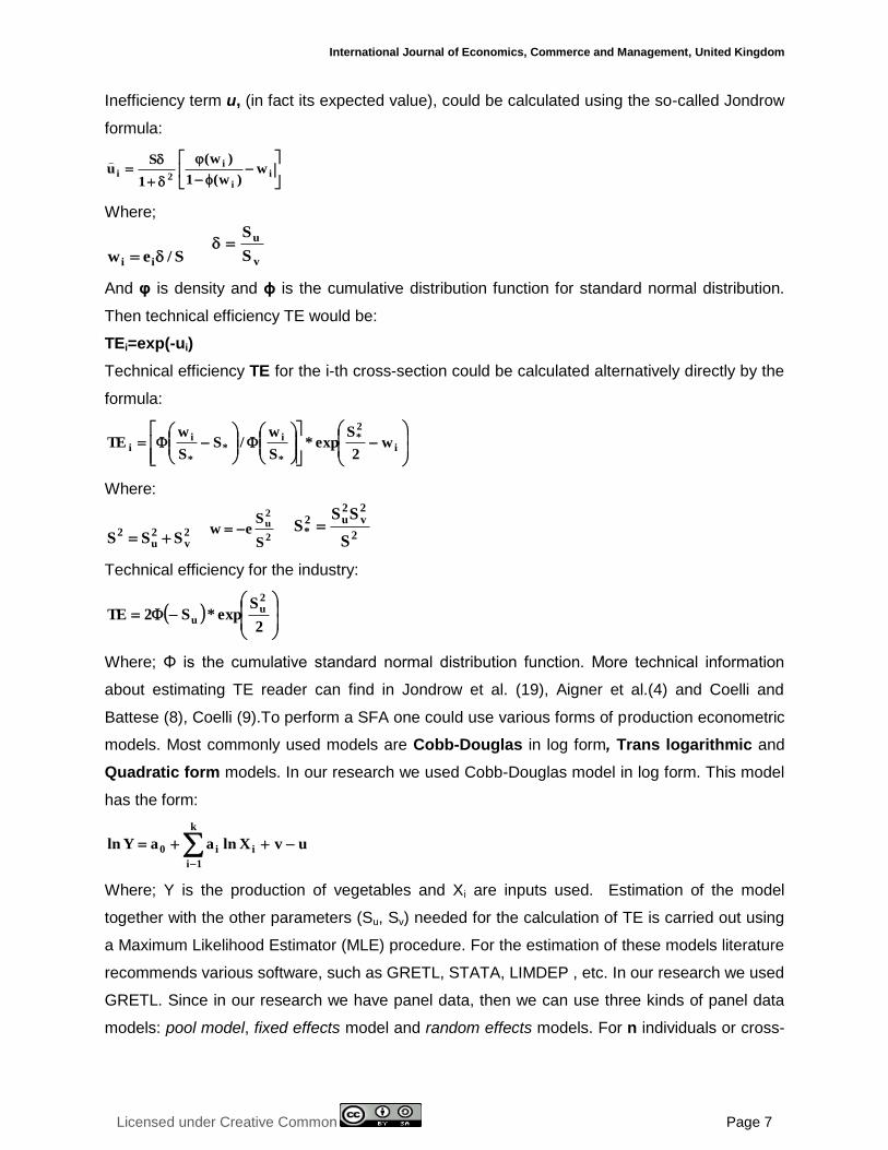
Inefficiency term u, (in fact its expected value), could be calculated using the so-called Jondrow

formula:

i

i

i

2i w)w(1

)w(

1

Su

Where;

S/ew ii v

u

S

S

And φ is density and ϕ is the cumulative distribution function for standard normal distribution.

Then technical efficiency TE would be:

TEi=exp(-ui)

Technical efficiency TE for the i-th cross-section could be calculated alternatively directly by the

formula:

i

2*

*

i*

*

ii w

2

Sexp*

S

w/S

S

wTE

Where:

2v

2u

2SSS

2

2u

S

Sew

2

2v

2u2

*S

SSS

Technical efficiency for the industry:

2

Sexp*S2TE

2u

u

Where; Φ is the cumulative standard normal distribution function. More technical information

about estimating TE reader can find in Jondrow et al. (19), Aigner et al.(4) and Coelli and

Battese (8), Coelli (9).To perform a SFA one could use various forms of production econometric

models. Most commonly used models are Cobb-Douglas in log form, Trans logarithmic and

Quadratic form models. In our research we used Cobb-Douglas model in log form. This model

has the form:

k

1i

ii0 uvXlnaaYln

Where; Y is the production of vegetables and Xi are inputs used. Estimation of the model

together with the other parameters (Su, Sv) needed for the calculation of TE is carried out using

a Maximum Likelihood Estimator (MLE) procedure. For the estimation of these models literature

recommends various software, such as GRETL, STATA, LIMDEP , etc. In our research we used

GRETL. Since in our research we have panel data, then we can use three kinds of panel data

models: pool model, fixed effects model and random effects models. For n individuals or cross-

http://ijecm.co.uk/



sections and T periods of time we have nT observations for each variable. The pool model

assumes no differences between individuals and time periods (years in our case) and it is:

ititit ebXaY

The fixed effects (FE) model is: ititiit ebX)aa(Y

In FE models the coefficient b is fixed, whereas coefficients ai reflect, if any, individual

differences. No time-invariant independent variables can be included in this model.

The random effects (RE) model is: )eu(bXaY itiitit

In RE models individual differences, if any, are reflected by ui. No correlation between X-is and

ui is assumed for this model. For more information about panel data models we recommend

(Gujarati, 2003), (Wooldridge, 2009), (GRETL User's Guide, 2012) and (FRONTIER 4.1 by

Coelli, 1995). Variables used, their scale of measurement and mode of their operationalization

are presented in the following table:

Table 1: Variables and their description and operationalization

Variable Description Scale of

measurement

Operationalization

Technical efficiency Level of efficiency Ratio A coefficient from 0 to 1

Vegetable production (LQ) Amount vegetables output Ratio Quintals

Land with vegetables (LS) Amount of land used for

vegetable production

Ratio Hectares

Number of tractors (LT) Number of tractors in use Ratio Pieces

Irrigation (Irrig) Percent of land potential for

irrigation

Ratio Percent of arable land

Climate (Clima) Climatic conditions in terms

of temperatures

Ordinal,

multinomial

0=Under 50 ha of greenhouses,

1=51-150 ha, 2=Above 150 ha

Working days (Wd) Number of working days

spent on farm

Ordinal, dummy 0=Under average, 1=Above

average

Farm size (Size) Amount of land used for

crops in hectares


average

Terrain (Terr) Amount of agriculture land

as percent to total land in a

given region

Ordinal, dummy 0=Under average % of

agriculture land to total land,

1=Above average

Fertilizer use (Fert) Amount of fertilizer used in

thousand ALL


average

We would like to use other variables as factors of efficiency, as literature suggests, like farmers'

education, technical assistance offered to farmers over years, cooperation, access to credits,

etc., but these data either don't exist or they are incomplete in terms of years or regions. For

some other variables we would like more accurate and reliable data, like farm capital, use of

fertilizers, farm labor, etc. These data are also are published in a non-systematic or inconsistent



form, some are incomplete, and we have been constringed to use proxy variables or dummies

instead of ratio scale variables. So the number of tractors (LT) is used as a proxy for farm

capital and the Working days (Wd) is used a proxy for labor. For all variables we gathered

regional-level secondary data for a 9-year period (2006-2009, 2011-2015) for each of 12 regions

of Albania. Thus, our data is a panel format of 9 periods and 12 cross-sections, with 108

observation altogether. Unfortunately, we didn't have access to data for most variables for year

2010, so our panel is incomplete. However, since our aim is to obtain average efficiency

estimates for the time horizon 2006-2015, a sample of 9 out of 10 years is sufficiently

representative.

RESULTS

According to our approach, land used for vegetables is the key and the only real factor of

production. The other factors or inputs, such as fertilizers, water for irrigation, etc. can only

upgrade land capacity to produce more, so they only can improve land efficiency.

As we discussed above, SFA uses ML estimator to obtain estimates of the model

parameters and variances of u and v components of the error term e. For this we need to know

which factors to include in the Cobb-Douglas production function and initial estimates for factor

regression coefficients. Since we have panel data, as a first step we discussed panel data

models. We have three major categories of panel data models: fixed effects (FE), random

effects (RE) and pool models. Since we have time-invariant variables such as Climate, Terrain,

etc., the fixed effect model might be excluded because it is inappropriate for that case, or we

can estimate the FE model excluding time-invariant variables. Then we estimated a RE model

including all input factors. The RE resulted:

Table 2: Random-effects (Generalized Least Squares), using 108 observations

Included 12 cross-sectional units, Time-series length = 9, Dependent variable: LQ

Coefficient Std. Error t-ratio p-value

Const 4.48514 0.528014 8.4943 <0.00001

LS 1.03867 0.0815821 12.7316 <0.00001

LT 0.0909095 0.0891018 1.0203 0.31005

Irrig -0.00191047 0.00396546 -0.4818 0.63102

Terr 0.116539 0.197652 0.5896 0.55678

Clima 0.0557291 0.180158 0.3093 0.75771

Wd 0.0146833 0.149144 0.0985 0.92177

Fert 0.0982861 0.195466 0.5028 0.61619

'Within' variance = 0.0124775; 'Between' variance = 0.0398248

Theta used for quasi-demeaning = 0.81342

http://ijecm.co.uk/



Breusch-Pagan test

Null hypothesis: Variance of the unit-specific error = 0

Asymptotic test statistic: Chi-square (1) = 72.7918

with p-value = 1.44073e-017

Hausman test

Null hypothesis: GLS estimates are consistent

Asymptotic test statistic: Chi-square (3) = 10.4329

with p-value = 0.0152233

Breusch-Pagan test rejects the null hypothesis of zero variance of the unit-specific error, so RE

is preferable to FE model. Hausman test rejects the null hypothesis of consistent GLS

estimates, so FE model is preferred to RE model. The FE model using only time-varying

variables results like this:

Table 3: Fixed-effects, using 108 observations

Included 12 cross-sectional units, Time-series length = 9, Dependent variable: LQ


Const 4.08968 0.652901 6.2639 <0.00001

LS 1.12854 0.0859189 13.1350 <0.00001

LT 0.0768708 0.106241 0.7236 0.47116

Irrig -0.00414483 0.00409752 -1.0115 0.31438

Mean dependent variable 13.14257 S.D. dependent variable 0.780168

Sum squared residuals 1.160404 S.E. of regression 0.111703

R-squared 0.982182 Adjusted R-squared 0.979500

F(14, 93) 366.1828 P-value(F) 8.99e-75

Log-likelihood 91.55623 Akaike criterion -153.1125

Schwarz criterion -112.8805 Hannan-Quinn -136.7999

Rho 0.468170 Durbin-Watson 0.879597

Test for differing group intercepts -

Null hypothesis: The groups have a common intercept

Test statistic: F (11, 93) = 14.9972

with p-value = P (F (11, 93) > 14.9972) = 2.7711e-016



The Fisher test rejects the null hypothesis that groups (regions in our case) have common

intercept, so the pool model is inappropriate. Both FE and RE model identify only land as a

significant factor to vegetables production. So we may choose between either FE or RE model

regression coefficients estimates.

If we exclude all insignificant factors and re-estimate the RE and FE models with only

land as independent variable the results would be:

Table 4: Re-estimated one-factor RE and FE models, dependent variable: LQ

RE model Coefficient Std. Error t-ratio p-value

Const 4.32548 0.486725 8.8869 <0.00001

LS 1.14554 0.0624768 18.3355 <0.00001

FE model R2=0.98

Const 4.28255 0.566887 7.5545 <0.00001

LS 1.15112 0.0736385 15.6321 <0.00001

For both models parameters are very close to each other. Both models are highly significant.

Relationship between land and vegetable production is elastic; one percent increase in land is

accompanied with 1.15% increase in production. Variability of land between regions is the

source of almost 98% of variability of production and all other remaining potential factors

contribute in total 2% of production variability among regions. How could be explained this result

of only land being so influential? One plausible explanation might be that their effect on

production is embedded in the effect of land and goes to production amount through land.

Then we used estimated parameters as initial estimates for a MLE estimation procedure,

to obtain new estimates of the parameters as well as estimation of standard deviations for u and

v terms. The results of estimations are:

Table 5: MLE, using observations 1-108

logl = ln(cnorm(e*lambda/ss)) - (ln(ss) + 0.5*(e/ss)^2)

Standard errors based on Outer Products matrix

Parameter Estimate Std. error p-value

b0 4.2347 0.390507 1.97e-027 ***

b1 1.12807 0.0442247 1.62e-143 ***

Su 0.278068 0.0641697 4.75e-05 ***

Sv 0.200520 0.0572199 0.0005 ***

Log-likelihood 16.61045 Akaike criterion -25.22090

Schwarz criterion -14.49237 Hannan-Quinn -20.87087

http://ijecm.co.uk/



Now we calculate:

0.117484=S2

S=0.34276, 026445.0S2* , 162618.0S*

66.0S

S

2

2u

γ=66% is telling that 66% of the error term variance is dedicated to variance in inefficiency. The

inefficiency variance is significant, meaning that inefficiency is statistically influencing regions'

vegetables output along the study period.

Next we calculate w (not shown here). The following table shows results on technical

efficiency by year and region.

Table 6: Efficiency scores for land used for vegetable production by year and region

Region 2006 2007 2008 2009 2011 2012 2013 2014 2015 Mean

Berat 0.954 0.948 0.957 0.957 0.956 0.955 0.953 0.951 0.958 0.954

Dibër 0.941 0.927 0.917 0.946 0.949 0.950 0.947 0.943 0.947 0.941

Durrës 0.898 0.920 0.926 0.910 0.935 0.930 0.912 0.925 0.927 0.920

Elbasan 0.881 0.882 0.899 0.899 0.936 0.942 0.930 0.932 0.935 0.915

Fier 0.917 0.924 0.932 0.935 0.948 0.948 0.935 0.944 0.947 0.937

Gjirokastër 0.808 0.770 0.816 0.785 0.881 0.872 0.874 0.865 0.866 0.837

Korçë 0.932 0.943 0.935 0.929 0.917 0.913 0.924 0.929 0.932 0.928

Kukës 0.917 0.911 0.916 0.903 0.911 0.919 0.917 0.911 0.918 0.913

Lezhë 0.907 0.916 0.913 0.917 0.893 0.912 0.912 0.922 0.920 0.912

Shkodër 0.892 0.886 0.886 0.887 0.890 0.876 0.871 0.877 0.888 0.884

Tiranë 0.829 0.830 0.879 0.862 0.871 0.871 0.846 0.861 0.878 0.859

Vlorë 0.923 0.924 0.915 0.901 0.896 0.892 0.850 0.878 0.896 0.897

Mean 0.900 0.898 0.907 0.903 0.915 0.915 0.906 0.911 0.918 0.908

On a national scale, efficiency is about 91%, and inefficiency about 9%. This result reflects

prevailing conditions in the study period. This means that under the given amount of inputs and

existing technology, farmers‟ knowledge and skills, business environment etc., there is little to

be done to further improve technical efficiency, because at maximum it can be improved by only

9%. In other words, to achieve the same amount of product, nationally could be saved at

maximum 9% of the current input base. Some regions can do more, but others much less.



Figure 3: Technical efficiency by years

Nationally, technical efficiency shows a positive trend, though not a strong one.

Figure 4: Technical efficiency by regions

Berat, Diber, Fier and Korca are consistently the most efficient regions, and Gjirokastra, Tirana

and Vlora are consistently the least efficient.

The last model we estimated is the model of efficiency to identify which are factors that

affect the level of efficiency (Tables 7 and 8):

Table 7: Heteroskedasticity-corrected TE model using observations 1-108


Const 0.664056 0.0351044 18.9166 <0.00001

LT 0.0359194 0.00595533 6.0315 <0.00001

Irrig 0.00108535 0.000312159 3.4769 0.00075

Terr 0.00638209 0.00737326 0.8656 0.38880

Clima 0.0287008 0.00636861 4.5066 0.00002

Size -0.0836689 0.00894942 -9.3491 <0.00001

Wd 0.0488113 0.00841832 5.7982 <0.00001

Fert -0.0207248 0.00688663 -3.0094 0.00331

0.885

0.89

0.895

0.9

0.905

0.91

0.915

0.92

1 2 3 4 5 6 7 8 9

0.75

0.8

0.85

0.9

0.95

1

http://ijecm.co.uk/



TE=0.664+9.0359*LT+0.00108*Irrig+0.00638*Terr+0.0287*Clima=0.0488*Size+0.0488*Wd-

0.02072*Fert+ε

Table 8: Statistics based on the weighted data:

Sum squared residuals 352.3981 S.E. of regression 1.877227

R-squared 0.572852 Adjusted R-squared 0.542951

F(7, 100) 19.15867 P-value(F) 5.05e-16

Log-likelihood -217.1074 Akaike criterion 450.2148

Schwarz criterion 471.6718 Hannan-Quinn 458.9148

All factors included in the model result statistically significant, except for Terrain, so Terrain

doesn‟t affect significantly amount of vegetable production. Size of farm and use of fertilizers are

negatively associated with vegetables output; smaller farms and those using less fertilizers

seem more efficient. Capital, Labor, and irrigation are positively associated with amount of

vegetable production. Climatic conditions, which may coincide with more intensive production

systems, also affect production positively.

CONCLUSIONS AND DISCUSSION

Doing this research we assume that all variables are measured without errors; otherwise,

results would reflect also such errors. Data come from the Ministry of Agriculture and/or the

Institute of Statistics, which are the official producers and distributors of the data.

Variables included are all aggregates representing regional levels. This means that

areas planted with specific vegetables and therefore their production for different vegetables

and different farms are hidden. Thus, it would be interesting and at the same time very useful to

further investigate the efficiency measure for specific vegetables on farm level data as well.

A key finding of our study is that efficiency scores seem for almost every region very

similar. This means that regions in Albania on the average do not differ substantially in terms of

the efficiency of use of available resources; in other words, under the existing economic,

technical, technology, social and environment conditions there is no room for much higher

technical efficiency. Or, said differently, if another country has lower efficiency score this doesn‟t

mean that in absolute terms its productivity is lower than that of Albania. Similar regional

efficiency score might be because of similarity of factors that affect efficiency, or because the

combined effect of these factors is similar for a large part of farms. Furthermore, despite this,

within regions there might be farms with large differences in their technical efficiency.

Another explanation of this finding could be the low input base for majority of Albanian

farms. If we refer to (World Development Indicators, 2017), Albania is using about 90 kg of



fertilizers per hectare of arable land, while Greece is using 160 kg, UK and Netherlands are

using about 240 kg. At low input use production per unit of inputs, or average production per

unit of input use could be higher. If farm resources are scarce farmers try to do use them with

utmost care. But this reveals a critical need for the Albanian farmers, the need to increase use

of inputs for more production and associated perhaps with high efficiency. More theoretically, as

the law of diminishing returns states, as the use of an input increases, for a given technology

and other inputs fixed, a point is reached after which other additions of input result in output

decrease; in other words, marginal product is decreasing. If technology improves, though law of

diminishing returns holds, production per unit of input or productivity increases and so it is

expected to happen with the technical efficiency scores. For large amounts of inputs, part of

them might be superfluous, or be inefficient, because of management difficulties, more complex

operations, resulting so in decreasing marginal product and also in the total product and

productivity. This may also lead to lower efficiency scores for the input used. For a more in

depth discussion see (Pindyck and Rubinfed, 1989), (Carrol, 1983), Debertin, 2012a, 2012b).

To conclude, efficiency of vegetable production in Albania results on the average high,

with remarkable fluctuations from region to region. Nationally the efficiency score is roughly 0.9,

with the highest peak region of Berat with the score of 0.954 and the lowest value that of

Gjirokastra with the score of 0.837. Its trend is positive with moderate increases and fluctuations

over years. One possible explanation of this result is that the input base of most Albanian

farmers is low and they do operate in the irrational range of input use, where the production

elasticity is greater than one.

As expected, land used for vegetable results a very powerful and significant factor for

their production. Almost 98% of production variation among regions is related with variation of

land area. Practically this means that it suffices to add the amount of land and this is translated

into more production. This may mean also that inputs‟ and technology base in different regions

base is similar, otherwise land increase in different regions would produce different output

volume.

Efficiency of vegetable production in Albania results significantly and positively

dependent on farm capital used, irrigation, amount of labor used and climatic conditions, or

intensity of production systems. Size of farms affects negatively the efficiency, meaning that

smaller farms are more efficient; this may be due to the better use and higher care for the use of

inputs by smaller farms because they are also poorer. Fertilizer use also affects negatively the

efficiency. This may be due to the fact that larger amounts of fertilizers need higher

management and technical skills and more knowledge to scale it up during the production

process and effectively combine them with other inputs such water, insecticides, manure, etc.

http://ijecm.co.uk/



This reveals an important problem, the need for better and systematic technical assistance to

farmers for the use of inputs, fertilizers included, and production techniques what would possibly

lead to higher technical efficiency.

Our findings confirm findings of other empirical research about a number of factors of

technical efficiency. This is about capital, irrigation, farm size, labor and climatic conditions such

as temperatures. But we couldn‟t assess the effect a number of other factors, such as

availability and quality of extension service, access to farm credit, education and age of farmers,

etc. This result underlines the need for a more comprehensive study on technical efficiency, in

terms of number and type of factors, but also type of products to be taken into consideration.

SCOPE FOR FURTHER RESEARCH

An assessment of technical efficiency based on farm level data is more than necessary in

Albania. This could provide more information about more factors affecting technical efficiency as

literature suggests and in many instances also confirms empirically. But this needs information

on the relevant variables. In Albania there is an alarming deficit of data about these variables;

so we urge government to thoroughly evaluate the agriculture information system and make

possible collection and publication of systematic country-level and regional disaggregated data

about use and prices of fertilizers, pesticides and insecticides, water for irrigation, technical

assistance to farmers, use of good agricultural practices, human capital, on-farm capital, access

to agriculture credits, etc. In a more comprehensive study, we suggest SFA methodology to

assess inefficiency in other crops, fruit-tree and animal husbandry. This could provide a more

general and detailed framework of efficiency level in the agriculture sector of Albania.

REFERENCES

Abate, G.T., Francesconi, G.N., Getnet, K. (2014). Impact of agricultural cooperation on smallholders/ technical efficiency; empirical evidence from Ethiopia, Annals of Public and Cooperative Economics 85:2 2014 pp. 1–30

Addai, K. N., Owusu,V., Danso-Abbeam A. G. ( (2014). Effects of Farmer – Based- Organization on the Technical efficiency of Maize Farmers across Various Agro - Ecological Zones of Ghana, Journal of Economics and Development Studies March 2014, Vol. 2, No. 1, pp. 141–161, USA

Adem, M., Gebregziabher, K. (2014). The effect of agricultural extension program on technical efficiency of rural farm households –evidence from northern Ethiopia: Stochastic Frontier Approach, International Researchers Volume No.3 Issue No.3 September, 2014

Aigner, D., Lovell, C.A., and Schimidt, (1977). Formulation and Estimation of stochastic frontier production models. Journal of Econometrics 6:21-32 (1992).

Anang, B.T., Bäckman, S., Sipiläinen, T. (2016). Agricultural microcredit and technical efficiency: The case of smallholder rice farmers in Northern Ghana, Journal of Agriculture and Rural Development in the Tropics and SubtropicsVol. 117 No. 2 (2016) 189–202, ISSN: 2363-6033 (online); 1612-9830 (print)



Bozog˘lu, M., Ceyhan, M. (2007). Measuring the technical efficiency and exploring the inefficiency determinants of vegetable farms in Samsun province, Turkey, Elsevier, Agricultural Systems 94 (2007) 649–656.

Carrol, Th.M. (1983). Microeconomic theory, concepts and applications, St. Martin Press, Inc., USA, pp 181-244

Coelli, T., Battese, G.(1996). Identification of factors which influence the technical efficiency of Indian farmers. Australian Journal of Agricultural Economics, 40 (August): 103-128.

Coelli, T.J,(1995). “A Guide to Frontier version 4.1c: A Computer program for Stochastic Frontier production and Cost Function Estimation”: Working paper 96/07, Centre for Efficiency and Productivity Analysis Dept. of Econometrics, University of New England

Darlington, S., Shumway, R.C., (2015). Analysis of Technical Change, Efficiency Change, and Total Factor Productivity Change , in U.S. Agriculture, School of Economic Sciences, Working Paper Series WP 2015-4

Debertin, D.L., (2012a). Agricultural Production Economics, Second edition, Amazon Createspace 2012, pp 431.

Debertin, D.L., (2012b). Applied Microeconomics Consumption, Production and Markets, pp 254.

Dinar, A., Karagiannis, G., Tzouvelekas, V.(2007). Evaluating the Impact of Public and Private Agricultural Extension on Farms Performance: A Non-neutral Stochastic Frontier Approach (Rural Development Dept, World Bank, USA), retrieved on date 12.04.2017 from: http://economics.soc.uoc.gr/wpa/docs/Extension.pdf

Elibariki E. M., Shuji, H. Tatsuhiko, N. (2008). An Analysis of Technical Efficiency of Smallholder Maize Farmers in Tanzania in the Globalization Era”. The XII World Congress of Rural Sociology of the International Rural Sociology Association, Goyang, Korea, 2008

Farrell, M.J. (1957). The Measurement of Productive Efficiency. Journal of the Royal Statistical Society, Series A, 120, 253-281. retrieved on date 10.06.2017 from: http://dx.doi.org/10.2307/2343100

Gretl User's Guide (2012), pp 133-139.

Gujarati, D. (2003). Basic Econometrics, 4-th edition, McGraw-Hill, Inc. pp 636-652 (ARDL)

Hazneci, E., Ceyhan, V. (2015). Measuring the Productive Efficiency and Identifying the Inefficiency Determinants of Dairy Farms in Amasya Province, Turkey. Journal of Agriculture and Environmental Sciences June 2015, Vol. 4, No. 1, pp. 100-107

Jondrow, J, C., Lovell, C.A, Materov, I.S.,Schmidt, P. (1982). “On the Estimation of Technical Efficiency in the stochastic Frontier Production Function Model”. Journal of Econometrics 19 no.2/3:233-38.

Khan, H.,Saeed, H. (2011). Measurement of Technical, Allocative and Economic Efficiency of Tomato Farms in Northern Pakistan, International Conference on Management, Economics and Social Sciences (ICMESS'2011) Bangkok December 2011

Kiprop, N.I.S., Bett K., Hillary, B.K., Mshenga, P., Nyairo, N. (2015). Analysis of Technical Efficiency among Smallholder Farmers in Kisii County, Kenya. IOSR Journal of Agriculture and Veterinary Science (IOSR-JAVS) e-ISSN: 2319-2380, p-ISSN: 2319-2372. Volume 8, Issue 3 Ver. I (Mar. 2015), PP 50-56

Kizito K. M., Malongo, R., Mlozi, S. (2015). Measuring Farm-level Technical Efficiency of Urban Agriculture inTanzanian Towns: The Policy Implications. World Journal of Social Science, Vol. 2, No. 1; 2015, E-ISSN 2329-9355 , retrieved on date 5.05.2017 from: URL: http://dx.doi.org/10.5430/wjss.v2n1p62

Madau, F.A. (2005). Technical Efficiency in Organic Farming: an Application on Italian Cereal Farms using a Parametric Approach, National Institute of Agricultural Economics (INEA) 07100 – Sassari (ITALY), presentation at the XIth Congress of the EAAE (European Association of Agricultural Economists), „The future of rural Europe in the global agri-food system‟, Copenhagen, Denmark, August 24-27, 2005

Pindyck, R.S., Rubinfeld, D.L. (1989). Microeconomics, Macmillan Publishing Company Inc, New York, pp 162-199

http://ijecm.co.uk/



Saldias, R., von Cramon-Taubadel, S. (2012). Access to Credit and the Determinants of Technical Inefficiency among Specialized Small Farmers in Chile, retrieved on date 3.05.2017 from: https://ideas.repec.org/p/zbw/daredp/1211.html

Simwaka, K., Ferrer, S., Harris G. (2013). Analysis of factors affecting technical efficiency of smallholder farmers: Comparing time-varying and time-invariant inefficiency models, African Journal of Agricultural Research, Vol. 8(29), pp. 3983-3993, 1 August, 2013

Theriault, V., Serra, R.(2013). Institutional Environment and Technical Efficiency: A Stochastic Frontier Analysis of Cotton Producers in West Africa, Journal of Agricultural Economics doi: 10.1111/1477-9552.12049

Wooldridge, G. (2009). Introductory Econometrics, 4-edition, South-Western Cengage Learning, pp 445-471

World Development Indicators (2017), retrieved on date 4.07.2017 from: http://data.worldbank.org/data-catalog/world-development-indicators

efficiency of vegetable production in …ijecm.co.uk/wp-content/uploads/2017/10/5102a.pdfliterature...

Documents