efficient algorithms for speech recognition
TRANSCRIPT
E�cient Algorithms for Speech Recognition
Mosur K. Ravishankar
May 15, 1996
CMU-CS-96-143
School of Computer ScienceComputer Science DivisionCarnegie Mellon University
Pittsburgh, PA 15213
Submitted in partial ful�llment of the requirements
for the degree of Doctor of Philosophy.
Thesis Committee:
Roberto Bisiani, co-chair (University of Milan)Raj Reddy, co-chairAlexander Rudnicky
Richard SternWayne Ward
c 1996 Mosur K. Ravishankar
This research was supported by the Department of the Navy, Naval Research Laboratory underGrant No. N00014-93-1-2005. The views and conclusions contained in this document are those ofthe author and should not be interpreted as representing the o�cial policies, either expressed orimplied, of the U.S. government.

Keywords: Speech recognition, search algorithms, real time recognition, lexicaltree search, lattice search, fast match algorithms, memory size reduction.
Abstract
Advances in speech technology and computing power have created a surge ofinterest in the practical application of speech recognition. However, the most accuratespeech recognition systems in the research world are still far too slow and expensive tobe used in practical, large vocabulary continuous speech applications. Their main goalhas been recognition accuracy, with emphasis on acoustic and language modelling.But practical speech recognition also requires the computation to be carried out inreal time within the limited resources|CPU power and memory size|of commonlyavailable computers. There has been relatively little work in this direction whilepreserving the accuracy of research systems.
In this thesis, we focus on e�cient and accurate speech recognition. It is easy toimprove recognition speed and reduce memory requirements by trading away accu-racy, for example by greater pruning, and using simpler acoustic and language models.It is much harder to improve both the recognition speed and reduce main memorysize while preserving the accuracy.
This thesis presents several techniques for improving the overall performance ofthe CMU Sphinx-II system. Sphinx-II employs semi-continuous hidden Markov mod-els for acoustics and trigram language models, and is one of the premier researchsystems of its kind. The techniques in this thesis are validated on several widely usedbenchmark test sets using two vocabulary sizes of about 20K and 58K words.
The main contributions of this thesis are an 8-fold speedup and 4-fold memory sizereduction over the baseline Sphinx-II system. The improvement in speed is obtainedfrom the following techniques: lexical tree search, phonetic fast match heuristic, andglobal best path search of the word lattice. The gain in speed from the tree search isabout a factor of 5. The phonetic fast match heuristic speeds up the tree search byanother factor of 2 by �nding the most likely candidate phones active at any time.Though the tree search incurs some loss of accuracy, it also produces compact wordlattices with low error rate which can be rescored for accuracy. Such a rescoring iscombined with the best path algorithm to �nd a globally optimum path through aword lattice. This recovers the original accuracy of the baseline system. The totalrecognition time is about 3 times real time for the 20K task on a 175MHz DEC Alphaworkstation.
The memory requirements of Sphinx-II are minimized by reducing the sizes ofthe acoustic and language models. The language model is maintained on disk andbigrams and trigrams are read in on demand. Explicit software caching mechanismse�ectively overcome the disk access latencies. The acoustic model size is reduced bysimply truncating precision of probability values to 8 bits. Several other engineeringsolutions, not explored in this thesis, can be applied to reduce memory requirementsfurther. The memory size for the 20K task is reduced to about 30-40MB.
i

ii
Acknowledgements
I cannot overstate the debt I owe to Roberto Bisiani and Raj Reddy. They havenot only helped me and given me every opportunity to extend my professional career,but also helped me through personal di�culties as well. It is quite remarkable that Ihave landed not one but two advisors that combine integrity towards research with ahuman touch that transcends the proverbial hard-headedness of science. One cannothope for better mentors than them. Alex Rudnicky, Rich Stern, and Wayne Ward,all have a clarity of thinking and self-expression that simply amazes me without end.They have given me the most insightful advice, comments, and questions that I couldhave asked for. Thank you, all.
The CMU speech group has been a pleasure to work with. First of all, I wouldlike to thank some former and current members, Mei-Yuh Hwang, Fil Alleva, LinChase, Eric Thayer, Sunil Issar, Bob Weide, and Roni Rosenfeld. They have helpedme through the early stages of my induction into the group, and later given invaluablesupport in my work. I'm fortunate to have inherited the work of Mei-Yuh and Fil.Lin Chase has been a great friend and sounding board for ideas through these years.Eric has been all of that and a great o�cemate. I have learnt a lot from discussionswith Paul Placeway. The rest of the speech group and the robust gang has made it amost lively environment to work in. I hope the charge continues through Sphinx-IIIand beyond.
I have spent a good fraction of my life in the CMU-CS community so far. It hasbeen, and still is, the greatest intellectual environment. The spirit of cooperation, andinformality of interactions as simply unique. I would like to acknowledge the supportof everyone I have ever come to know here, too many to name, from the Warp andNectar days until now. The administrative folks have always succeeded in bluntingthe edge o� a di�cult day. You never know what nickname Catherine Copetas willchristen you with next. And Sharon Burks has always put up with all my antics.
It goes without saying that I owe everything to my parents. I have had tremendoussupport from my brothers, and some very special uncles and aunts. In particular, Imust mention the fun I've had with my brother Kuts. I would also like to acknowledgeK. Gopinath's help during my stay in Bangalore. Finally, \BB", who has su�eredthrough my tantrums on bad days, kept me in touch with the rest of the world, has amost creative outlook on the commonplace, can drive me nuts some days, but whenall is said and done, is a most relaxed and comfortable person to have around.
Last but not least, I would like to thank Andreas Nowatzyk, Monica Lam, DuaneNorthcutt and Ray Clark. It has been my good fortune to witness and participate insome of Andreas's creative work. This thesis owes a lot to his unending support andencouragement.
iii

iv
Contents
Abstract i
Acknowledgements iii
1 Introduction 1
1.1 The Modelling Problem : : : : : : : : : : : : : : : : : : : : : : : : : 3
1.2 The Search Problem : : : : : : : : : : : : : : : : : : : : : : : : : : : 5
1.3 Thesis Contributions : : : : : : : : : : : : : : : : : : : : : : : : : : : 7
1.3.1 Improving Speed : : : : : : : : : : : : : : : : : : : : : : : : : 8
1.3.2 Reducing Memory Size : : : : : : : : : : : : : : : : : : : : : : 8
1.4 Summary and Dissertation Outline : : : : : : : : : : : : : : : : : : : 9
2 Background 11
2.1 Acoustic Modelling : : : : : : : : : : : : : : : : : : : : : : : : : : : : 11
2.1.1 Phones and Triphones : : : : : : : : : : : : : : : : : : : : : : 11
2.1.2 HMM modelling of Phones and Triphones : : : : : : : : : : : 12
2.2 Language Modelling : : : : : : : : : : : : : : : : : : : : : : : : : : : 13
2.3 Search Algorithms : : : : : : : : : : : : : : : : : : : : : : : : : : : : 15
2.3.1 Viterbi Beam Search : : : : : : : : : : : : : : : : : : : : : : : 15
2.4 Related Work : : : : : : : : : : : : : : : : : : : : : : : : : : : : : : : 17
2.4.1 Tree Structured Lexicons : : : : : : : : : : : : : : : : : : : : : 17
2.4.2 Memory Size and Speed Improvements in Whisper : : : : : : 19
2.4.3 Search Pruning Using Posterior Phone Probabilities : : : : : : 20
v
2.4.4 Lower Complexity Viterbi Algorithm : : : : : : : : : : : : : : 20
2.5 Summary : : : : : : : : : : : : : : : : : : : : : : : : : : : : : : : : : 21
3 The Sphinx-II Baseline System 22
3.1 Knowledge Sources : : : : : : : : : : : : : : : : : : : : : : : : : : : : 24
3.1.1 Acoustic Model : : : : : : : : : : : : : : : : : : : : : : : : : : 24
3.1.2 Pronunciation Lexicon : : : : : : : : : : : : : : : : : : : : : : 26
3.2 Forward Beam Search : : : : : : : : : : : : : : : : : : : : : : : : : : 26
3.2.1 Flat Lexical Structure : : : : : : : : : : : : : : : : : : : : : : 26
3.2.2 Incorporating the Language Model : : : : : : : : : : : : : : : 27
3.2.3 Cross-Word Triphone Modeling : : : : : : : : : : : : : : : : : 28
3.2.4 The Forward Search : : : : : : : : : : : : : : : : : : : : : : : 31
3.3 Backward and A* Search : : : : : : : : : : : : : : : : : : : : : : : : : 36
3.3.1 Backward Viterbi Search : : : : : : : : : : : : : : : : : : : : : 37
3.3.2 A* Search : : : : : : : : : : : : : : : : : : : : : : : : : : : : : 37
3.4 Baseline Sphinx-II System Performance : : : : : : : : : : : : : : : : : 38
3.4.1 Experimentation Methodology : : : : : : : : : : : : : : : : : : 39
3.4.2 Recognition Accuracy : : : : : : : : : : : : : : : : : : : : : : 41
3.4.3 Search Speed : : : : : : : : : : : : : : : : : : : : : : : : : : : 42
3.4.4 Memory Usage : : : : : : : : : : : : : : : : : : : : : : : : : : 45
3.5 Baseline System Summary : : : : : : : : : : : : : : : : : : : : : : : : 48
4 Search Speed Optimization 49
4.1 Motivation : : : : : : : : : : : : : : : : : : : : : : : : : : : : : : : : : 49
4.2 Lexical Tree Search : : : : : : : : : : : : : : : : : : : : : : : : : : : : 51
4.2.1 Lexical Tree Construction : : : : : : : : : : : : : : : : : : : : 54
4.2.2 Incorporating Language Model Probabilities : : : : : : : : : : 56
4.2.3 Outline of Tree Search Algorithm : : : : : : : : : : : : : : : : 61
4.2.4 Performance of Lexical Tree Search : : : : : : : : : : : : : : : 62
4.2.5 Lexical Tree Search Summary : : : : : : : : : : : : : : : : : : 67
vi
4.3 Global Best Path Search : : : : : : : : : : : : : : : : : : : : : : : : : 68
4.3.1 Best Path Search Algorithm : : : : : : : : : : : : : : : : : : : 68
4.3.2 Performance : : : : : : : : : : : : : : : : : : : : : : : : : : : : 73
4.3.3 Best Path Search Summary : : : : : : : : : : : : : : : : : : : 74
4.4 Rescoring Tree-Search Word Lattice : : : : : : : : : : : : : : : : : : : 76
4.4.1 Motivation : : : : : : : : : : : : : : : : : : : : : : : : : : : : : 76
4.4.2 Performance : : : : : : : : : : : : : : : : : : : : : : : : : : : : 76
4.4.3 Summary : : : : : : : : : : : : : : : : : : : : : : : : : : : : : 78
4.5 Phonetic Fast Match : : : : : : : : : : : : : : : : : : : : : : : : : : : 78
4.5.1 Motivation : : : : : : : : : : : : : : : : : : : : : : : : : : : : : 78
4.5.2 Details of Phonetic Fast Match : : : : : : : : : : : : : : : : : 80
4.5.3 Performance of Fast Match Using All Senones : : : : : : : : : 84
4.5.4 Performance of Fast Match Using CI Senones : : : : : : : : : 87
4.5.5 Phonetic Fast Match Summary : : : : : : : : : : : : : : : : : 88
4.6 Exploiting Concurrency : : : : : : : : : : : : : : : : : : : : : : : : : 89
4.6.1 Multiple Levels of Concurrency : : : : : : : : : : : : : : : : : 90
4.6.2 Parallelization Summary : : : : : : : : : : : : : : : : : : : : : 93
4.7 Summary of Search Speed Optimization : : : : : : : : : : : : : : : : 93
5 Memory Size Reduction 97
5.1 Senone Mixture Weights Compression : : : : : : : : : : : : : : : : : : 97
5.2 Disk-Based Language Models : : : : : : : : : : : : : : : : : : : : : : 98
5.3 Summary of Experiments on Memory Size : : : : : : : : : : : : : : : 100
6 Small Vocabulary Systems 101
6.1 General Issues : : : : : : : : : : : : : : : : : : : : : : : : : : : : : : : 101
6.2 Performance on ATIS : : : : : : : : : : : : : : : : : : : : : : : : : : : 102
6.2.1 Baseline System Performance : : : : : : : : : : : : : : : : : : 102
6.2.2 Performance of Lexical Tree Based System : : : : : : : : : : : 103
6.3 Small Vocabulary Systems Summary : : : : : : : : : : : : : : : : : : 106
vii
7 Conclusion 107
7.1 Summary of Results : : : : : : : : : : : : : : : : : : : : : : : : : : : 108
7.2 Contributions : : : : : : : : : : : : : : : : : : : : : : : : : : : : : : : 109
7.3 Future Work on E�cient Speech Recognition : : : : : : : : : : : : : : 111
Appendices
A The Sphinx-II Phone Set 115
B Statistical Signi�cance Tests 116
B.1 20K Task : : : : : : : : : : : : : : : : : : : : : : : : : : : : : : : : : 117
B.2 58K Task : : : : : : : : : : : : : : : : : : : : : : : : : : : : : : : : : 121
Bibliography 125
viii
List of Figures
2.1 Viterbi Search as Dynamic Programming : : : : : : : : : : : : : : : : 15
3.1 Sphinx-II Signal Processing Front End. : : : : : : : : : : : : : : : : : 24
3.2 Sphinx-II HMM Topology: 5-State Bakis Model. : : : : : : : : : : : : 25
3.3 Cross-word Triphone Modelling at Word Ends in Sphinx-II. : : : : : : 29
3.4 Word Initial Triphone HMM Modelling in Sphinx-II. : : : : : : : : : 31
3.5 One Frame of Forward Viterbi Beam Search in the Baseline System. : 33
3.6 Word Transitions in Sphinx-II Baseline System. : : : : : : : : : : : : 35
3.7 Outline of A* Algorithm in Baseline System : : : : : : : : : : : : : : 38
3.8 Language Model Structure in Baseline Sphinx-II System. : : : : : : : 46
4.1 Basephone Lexical Tree Example. : : : : : : : : : : : : : : : : : : : : 52
4.2 Triphone Lexical Tree Example. : : : : : : : : : : : : : : : : : : : : : 55
4.3 Cross-Word Transitions With Flat and Tree Lexicons. : : : : : : : : : 57
4.4 Auxiliary Flat Lexical Structure for Bigram Transitions. : : : : : : : 58
4.5 Path Score Adjustment Factor f for Word wj Upon Its Exit. : : : : : 59
4.6 One Frame of Forward Viterbi Beam Search in Tree Search Algorithm. 63
4.7 Word Lattice for Utterance: Take Fidelity's case as an example. : : : 69
4.8 Word Lattice Example Represented as a DAG. : : : : : : : : : : : : : 70
4.9 Word Lattice DAG Example Using a Trigram Grammar. : : : : : : : 71
4.10 Suboptimal Usage of Trigrams in Sphinx-II Viterbi Search. : : : : : : 73
4.11 Base Phones Predicted by Top Scoring Senones in Each Frame; SpeechFragment for Phrase THIS TREND, Pronounced DH-IX-S T-R-EH-N-DD. : : : : : : : : : : : : : : : : : : : : : : : : : : : : : : : : : : : 81
ix
4.12 Position of Correct Phone in Ranking Created by Phonetic Fast Match. 82
4.13 Lookahead Window for Smoothing the Active Phone List. : : : : : : 83
4.14 Phonetic Fast Match Performance Using All Senones (20K Task). : : 85
4.15 Word Error Rate vs Recognition Speed of Various Systems. : : : : : : 94
4.16 Con�guration of a Practical Speech Recognition System. : : : : : : : 95
x
List of Tables
3.1 No. of Words and Sentences in Each Test Set : : : : : : : : : : : : : 40
3.2 Percentage Word Error Rate of Baseline Sphinx-II System. : : : : : : 41
3.3 Overall Execution Times of Baseline Sphinx-II System (xRealTime). : 43
3.4 Baseline Sphinx-II System Forward Viterbi Search Execution Times(xRealTime). : : : : : : : : : : : : : : : : : : : : : : : : : : : : : : : 43
3.5 HMMs Evaluated Per Frame in Baseline Sphinx-II System. : : : : : : 44
3.6 N -gram Transitions Per Frame in Baseline Sphinx-II System. : : : : : 45
4.1 No. of Nodes at Each Level in Tree and Flat Lexicons. : : : : : : : : 55
4.2 Execution Times for Lexical Tree Viterbi Search. : : : : : : : : : : : 64
4.3 Breakdown of Tree Viterbi Search Execution Times (xRealTime). : : 65
4.4 No. of HMMs Evaluated Per Frame in Lexical Tree Search. : : : : : : 65
4.5 No. of Language Model Operations/Frame in Lexical Tree Search. : : 65
4.6 Word Error Rates for Lexical Tree Viterbi Search. : : : : : : : : : : : 66
4.7 Word Error Rates from Global Best Path Search of Word Lattice Pro-duced by Lexical Tree Search. : : : : : : : : : : : : : : : : : : : : : : 74
4.8 Execution Times for Global Best Path DAG Search (x RealTime). : : 74
4.9 Word Error Rates From Lexical Tree+Rescoring+Best Path Search. : 77
4.10 Execution Times With Rescoring Pass. : : : : : : : : : : : : : : : : : 77
4.11 Fast Match Using All Senones; Lookahead Window=3 (20K Task). : : 86
4.12 Fast Match Using All Senones; Lookahead Window=3 (58K Task). : : 87
4.13 Fast Match Using CI Senones; Lookahead Window=3. : : : : : : : : : 88
6.1 Baseline System Performance on ATIS. : : : : : : : : : : : : : : : : : 103
xi
6.2 Ratio of Number of Root HMMs in Lexical Tree and Words in Lexicon(approximate). : : : : : : : : : : : : : : : : : : : : : : : : : : : : : : 103
6.3 Execution Times on ATIS. : : : : : : : : : : : : : : : : : : : : : : : : 104
6.4 Breakdown of Tree Search Execution Times on ATIS (Without Pho-netic Fast Match). : : : : : : : : : : : : : : : : : : : : : : : : : : : : 104
6.5 Recognition Accuracy on ATIS. : : : : : : : : : : : : : : : : : : : : : 105
A.1 The Sphinx-II Phone Set. : : : : : : : : : : : : : : : : : : : : : : : : 115
xii
Chapter 1
Introduction
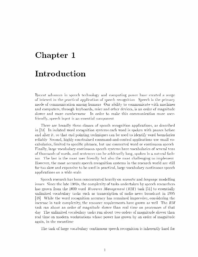
Recent advances in speech technology and computing power have created a surgeof interest in the practical application of speech recognition. Speech is the primarymode of communication among humans. Our ability to communicate with machinesand computers, through keyboards, mice and other devices, is an order of magnitudeslower and more cumbersome. In order to make this communication more user-friendly, speech input is an essential component.
There are broadly three classes of speech recognition applications, as describedin [53]. In isolated word recognition systems each word is spoken with pauses beforeand after it, so that end-pointing techniques can be used to identify word boundariesreliably. Second, highly constrained command-and-control applications use small vo-cabularies, limited to speci�c phrases, but use connected word or continuous speech.Finally, large vocabulary continuous speech systems have vocabularies of several tensof thousands of words, and sentences can be arbitrarily long, spoken in a natural fash-ion. The last is the most user-friendly but also the most challenging to implement.However, the most accurate speech recognition systems in the research world are stillfar too slow and expensive to be used in practical, large vocabulary continuous speechapplications on a wide scale.
Speech research has been concentrated heavily on acoustic and language modellingissues. Since the late 1980s, the complexity of tasks undertaken by speech researchershas grown from the 1000-word Resource Management (RM) task [51] to essentiallyunlimited vocabulary tasks such as transcription of radio news broadcast in 1995[48]. While the word recognition accuracy has remained impressive, considering theincrease in task complexity, the resource requirements have grown as well. The RMtask ran about an order of magnitude slower than real time on processors of thatday. The unlimited vocabulary tasks run about two orders of magnitude slower thanreal time on modern workstations whose power has grown by an order of magnitudeagain, in the meantime.
The task of large vocabulary continuous speech recognition is inherently hard for
1
2 CHAPTER 1. INTRODUCTION
the following reasons. First, word boundaries are not known in advance. One mustbe constantly prepared to encounter such a boundary at every time instant. We candraw a rough analogy to reading a paragraph of text without any punctuation marksor spaces between words:
myspiritwillsleepinpeaceorifthinksitwillsurelythinkthusfarewellhesprangfromthecabinwindowashesaidthisupontheiceraftwhichlayclosetothevesselhewassoonborneawaybythewavesandlostindarknessanddistance...
Furthermore, many incorrect word hypotheses will be produced from incorrect seg-mentation of speech. Sophisticated language models that provide word context orsemantic information are needed to disambiguate between the available hypotheses.
The second problem is that co-articulatory e�ects are very strong in natural orconversational speech, so that the sound produced at one instant is in uenced bythe preceding and following ones. Distinguishing between these requires the use ofdetailed acoustic models that take such contextual conditions into account. The in-creasing sophistication of language models and acoustic models, as well as the growthin the complexity of tasks, has far exceeded the computational and memory capacitiesof commonly available workstations.
E�cient speech recognition for practical applications also requires that the pro-cessing be carried out in real time within the limited resources|CPU power andmemory size|of commonly available computers. There certainly are various suchcommercial and demonstration systems in existence, but their performance has neverbeen formally evaluated with respect to the research systems or with respect to oneanother, in the way that the accuracy of research systems has been. This thesis isprimarily concerned with these issues|in improving the computational and memorye�ciency of current speech recognition technology without compromising the achieve-ments in recognition accuracy.
The three aspects of performance, recognition speed, memory resource require-ments, and recognition accuracy, are in mutual con ict. It is relatively easy to improverecognition speed and reduce memory requirements while trading away some accu-racy, for example by pruning the search space more drastically, and by using simpleracoustic and language models. Alternatively, one can reduce memory requirementsthrough e�cient encoding schemes at the expense of computation time needed to de-code such representations, and vice versa. But it is much harder to improve both therecognition speed and reduce main memory requirements while preserving or improv-ing recognition accuracy. In this thesis, we demonstrate algorithmic and heuristictechniques to tackle the problem.
This work has been carried out in the context of the CMU Sphinx-II speechrecognition system as a baseline. There are two main schools of speech recognitiontechnology today, based on statistical hidden Markov modelling (HMM), and neural
1.1. THE MODELLING PROBLEM 3
net technology, respectively. Sphinx-II uses HMM-based statistical modelling tech-niques and is one of the premier recognizers of its kind. Using several commonly usedbenchmark test sets and two di�erent vocabulary sizes of about 20,000 and 58,000words, we demonstrate that the recognition accuracy of the baseline Sphinx-II systemcan be attained while its execution time is reduced by about an order of magnitudeand memory requirements reduced by a factor of about 4.
1.1 The Modelling Problem
As the complexity of tasks tackled by speech research has grown, so has that ofthe modelling techniques. In systems that use statistical modelling techniques, suchas the Sphinx system, this translates into several tens to hundreds of megabytes ofmemory needed to store information regarding statistical distributions underlying themodels.
Acoustic Models
One of the key issues in acoustic modelling has been the choice of a good unit ofspeech [32, 27]. In small vocabulary systems of a few tens of words, it is possible tobuild separate models for entire words, but this approach quickly becomes infeasibleas the vocabulary size grows. For one thing, it is hard to obtain su�cient trainingdata to build all individual word models. It is necessary to represent words in termsof sub-word units, and train acoustic models for the latter, in such a way that thepronunciation of new words can be de�ned in terms of the already trained sub-wordunits.
The phoneme (or phone) has been the most commonly accepted sub-word unit.There are approximately 50 phones in spoken English language; words are de�ned assequences of such phones1 (see Appendix A for the Sphinx-II phone set and examples).Each phone is, in turn, modelled by an HMM (described in greater detail in Section2.1.2).
As mentioned earlier, natural continuous speech has strong co-articulatory ef-fects. Informally, a phone models the position of various articulators in the mouthand nasal passage (such as the tongue and the lips) in the making of a particularsound. Since these articulators have to move smoothly between di�erent sounds inproducing speech, each phone is in uenced by the neighbouring ones, especially dur-ing the transition from one phone to the next. This is not a major concern in smallvocabulary systems in which words are not easily confusable, but becomes an issueas the vocabulary size and the degree of confusability increase.
1Some systems de�ne word pronunciations as networks of phones instead of simple linear se-quences [36].
4 CHAPTER 1. INTRODUCTION
Most systems employ triphones as one form of context-dependent HMM models[4, 33] to deal with this problem. Triphones are basically phones observed in thecontext of given preceding and succeeding phones. There are approximately 50 phonesin spoken English language. Thus, there can be a total of about 503 triphones,although only a fraction of them are actually observed in the language. Limitingthe vocabulary can further reduce this number. For example, in Sphinx-II, a 20,000word vocabulary has about 75,000 distinct triphones, each of which is modelled by a5-state HMM, for a total of about 375,000 states. Since there isn't su�cient trainingdata to build models for each state, they are clustered into equivalence classes calledsenones [27].
The introduction of context-dependent acoustic models, even after clustering intoequivalence classes, creates an explosion in the memory requirements to store suchmodels. For example, the Sphinx-II system with 10,000 senones occupies tens ofmegabytes of memory.
Language Models
Large vocabulary continuous speech recognition requires the use of a language modelor grammar to select the most likely word sequence from the relatively large numberof alternative word hypotheses produced during the search process. As mentionedearlier, the absence of explicit word boundary markers in continuous speech causesseveral additional word hypotheses to be produced, in addition to the intended orcorrect ones. For example, the phrase It's a nice day can be equally well recognizedas It sun iced A. or It son ice day. They are all acoustically indistinguishable, but theword boundaries have been drawn at a di�erent set of locations in each case. Clearly,many more alternatives can be produced with varying degrees of likelihood, given theinput speech. The language model is necessary to pick the most likely sequence ofwords from the available alternatives.
Simple tasks, in which one is only required to recognize a constrained set ofphrases, can use rule-based regular or context-free grammars which can be repre-sented compactly. However, that is impossible with large vocabulary tasks. Instead,bigram and trigram grammars, consisting of word pairs and triples with given prob-abilities of occurrence, are most commonly used. One can also build such languagemodels based on word classes, such as city names, months of the year, etc. However,creating such grammars is tedious as they require a fair amount of hand compilationof the classes. Ordinary word n-gram language models, on the other hand, can becreated almost entirely automatically from a corpus of training text.
Clearly, it is infeasible to create a complete set of word bigrams for even mediumvocabulary tasks. Thus, the set of bigram and trigram probabilities actually presentin a given grammar is usually a small subset of the possible number. Even then, theyusually number in the millions for large vocabulary tasks. The memory requirements
1.2. THE SEARCH PROBLEM 5
for such language models range from several tens to hundreds of megabytes.
1.2 The Search Problem
There are two components to the computational cost of speech recognition: acousticprobability computation, and search. In the case of HMM-based systems, the formerrefers to the computation of the probability of a given HMM state emitting theobserved speech at a given time. The latter refers to the search for the best wordsequence given the complete speech input. The search cost is largely una�ected bythe complexity of the acoustic models. It is much more heavily in uenced by the sizeof the task. As we shall see later, the search cost is signi�cant for medium and largevocabulary recognition; it is the main focus of this thesis.
Speech recognition|searching for the most likely sequence of words given theinput speech|gives rise to an exponential search space if all possible sequences ofwords are considered. The problem has generally been tackled in two ways: Viterbidecoding [62, 52] using beam search [37], or stack decoding [9, 50] which is a variantof the A* algorithm [42]. Some hybrid versions that combine Viterbi decoding withthe A* algorithm also exist [21].
Viterbi Decoding
Viterbi decoding is a dynamic programming algorithm that searches the state spacefor the most likely state sequence that accounts for the input speech. The statespace is constructed by creating word HMM models from its constituent phone ortriphone HMM models, and all word HMM models are searched in parallel. Sincethe state space is huge for even medium vocabulary applications, the beam searchheuristic is usually applied to limit the search by pruning out the less likely states.The combination is often simply referred to as Viterbi beam search. Viterbi decodingis a time-synchronous search that processes the input speech one frame at a time,updating all the states for that frame before moving on to the next frame. Mostsystems employ a frame input rate of 100 frames/sec. Viterbi decoding is describedin greater detail in Section 2.3.1.
Stack Decoding
Stack decoding maintains a stack of partial hypotheses2 sorted in descending order ofposterior likelihood. At each step it pops the best one o� the stack. If it is a completehypothesis it is output. Otherwise the algorithm expands it by one word, trying all
2A partial hypothesis accounts for an initial portion of the input speech. A complete hypothesis,or simply hypothesis, accounts for the entire input speech.
6 CHAPTER 1. INTRODUCTION
possible word extensions, evaluates the resulting (partial) hypotheses with respectto the input speech and re-inserts them in the sorted stack. Any number of N -besthypotheses [59] can be generated in this manner. To avoid an exponential growth inthe set of possible word sequences in medium and large vocabulary systems, partialhypotheses are expanded only by a limited set of candidate words at each step. Thesecandidates are identi�ed by a fast match step [6, 7, 8, 20]. Since our experiments havebeen mostly con�ned to Viterbi decoding, we do not explore stack decoding in anygreater detail.
Tree Structured Lexicons
Even with the beam search heuristic, straightforward Viterbi decoding is expensive.The network of states to be searched is formed by a linear sequence of HMM modelsfor each word in the vocabulary. The number of models actively searched in thisorganization is still one to two orders of magnitude beyond the capabilities of modernworkstations.
Lexical trees can be used to reduce the size of the search space. Since manywords share common pronunciation pre�xes, they can also share models and avoidduplication. Trees were initially used in fast match algorithms for producing candidateword lists for further search. Recently, they have been introduced in the main searchcomponent of several systems [44, 39, 43, 3]. The main problem faced by them is inusing a language model. Normally, transitions between words are accompanied bya prior language model probability. But with trees, the destination nodes of suchtransitions are not individual words but entire groups of them, related phoneticallybut quite unrelated grammatically. An e�cient solution to this problem is one of theimportant contributions of this thesis.
Multipass Search Techniques
Viterbi search algorithms usually also create a word lattice in addition to the bestrecognition hypothesis. The lattice includes several alternative words that were recog-nized at any given time during the search. It also typically contains other informationsuch as the time segmentations for these words, and their posterior acoustic scores(i.e., the probability of observing a word given that time segment of input speech).The lattice error rate measures the number of correct words missing from the latticearound the expected time. It is typically much lower than the word error rate3 of thesingle best hypotheses produced for each sentence.
Word lattices can be kept very compact, with low lattice error rate, if they areproduced using su�ciently detailed acoustic models (as opposed to primitive models
3Word error rates are measured by counting the number of word substitutions, deletions, andinsertions in the hypothesis, compared to the correct reference sentence.
1.3. THESIS CONTRIBUTIONS 7
as in, for example, fast match algorithms). In our work, a 10sec long sentence typicallyproduces a word lattice containing about 1000 word instances.
Given such compact lattices with low error rates, one can search them usingsophisticated models and search algorithms very e�ciently and obtain results with alower word error rate, as described in [38, 65, 41]. Most systems use such multipasstechniques.
However, there has been relatively little work reported in actually creating suchlattices e�ciently. This is important for the practical applicability of such techniques.Lattices can be created with low computational overhead if we use simple models, buttheir size must be large to guarantee a su�ciently low lattice error rate. On the otherhand, compact, low-error lattices can be created using more sophisticated models, atthe expense of more computation time. The e�cient creation of compact, low-errorlattices for e�cient postprocessing is another byproduct of this work.
1.3 Thesis Contributions
This thesis explores ways of improving the performance of speech recognition systemsalong the dimensions of recognition speed and e�ciency of memory usage, whilepreserving the recognition accuracy of research systems. As mentioned earlier, thisis a much harder problem than if we are allowed to trade recognition accuracy forimprovement in speed and memory usage.
In order to make meaningful comparisons, the baseline performance of an estab-lished \research" system is �rst measured. We use the CMU Sphinx-II system as thebaseline system since it has been extensively used in the yearly ARPA evaluations.It has known recognition accuracy on various test sets, and with similarities to manyother research systems. The parameters measured include, in addition to recognitionaccuracy, the CPU usage of various steps during execution, frequency counts of themost time-consuming operations, and memory usage. All tests are carried out usingtwo vocabulary sizes of about 20,000 (20K) and 58,000 (58K) words, respectively.The test sentences are taken from the ARPA evaluations in 1993 and 1994 [45, 46].
The results from this analysis show that the search component is several tensof times slower than real time on the reported tasks. (The acoustic output proba-bility computation is relatively smaller since these tests have been conducted usingsemi-continuous acoustic models [28, 27].) Furthermore, the search time itself canbe further decomposed into two main components: the evaluation of HMM models,and carrying out cross-word transitions at word boundaries. The former is simply ameasure of the task complexity. The latter is a signi�cant problem since there arecross-word transitions to every word in the vocabulary, and language model proba-bilities must be computed for every one of them.
8 CHAPTER 1. INTRODUCTION
1.3.1 Improving Speed
The work presented in this thesis shows that a new adaptation of lexical tree searchcan be used to reduce both the number of HMMs evaluated and the cost of cross-wordtransitions. In this method, language model probabilities for a word are computed notwhen entering that word but upon its exit, if it is one of the recognized candidates.The number of such candidates at a given instant is on average about two orders ofmagnitude smaller than the vocabulary size. Furthermore, the proportion appears todecrease with increasing vocabulary size.
Using this method, the execution time for recognition is decreased by a factor ofabout 4.8 for both the 20K and 58K word tasks. If we exclude the acoustic outputprobability computation, the speedup of the search component alone is about 6.3 forthe 20K word task and over 7 for the 58K task. It also demonstrates that the lexicaltree search e�ciently produces compact word lattices with low error rates that canagain be e�ciently searched using more complex models and search algorithms.
Even though there is a relative loss of accuracy of about 20% using this method, weshow that it can be recovered e�ciently by postprocessing the word lattice producedby the lexical tree search. The loss is attributed to suboptimal word segmentationsproduced by the tree search. However, a new shortest-path graph search formulationfor searching the word lattice can reduce the loss in accuracy to under 10% relativeto the baseline system with a negligible increase in computation.
If the lattice is �rst rescored to obtain better word segmentations, all the loss inaccuracy is recovered. The rescoring step adds less than 20% execution time overhead,giving an e�ective overall speedup of about 4 over the baseline system.
We have applied a new phonetic fast match step to the lexical tree search thatperforms an initial pruning of the context independent phones to be searched. Thistechnique reduces the overall execution time by about 40-45%, with a less than 2%relative loss in accuracy. This brings the overall speed of the system to about 8 timesthat of the baseline system, with almost no loss of accuracy.
The structure of the �nal decoder is a pipeline of several stages which can beoperated in an overlapped fashion. Parallelism among stages, especially the lexicaltree search and rescoring passes, is possible for additional improvement in speed.
1.3.2 Reducing Memory Size
The two main candidates for memory usage in the baseline Sphinx-II system, andmost of the common research systems, are the acoustic and language models.
The key observation for reducing the size of the language models is that in decod-ing any given utterance, only a small portion of it is actually used. Hence, we can
1.4. SUMMARY AND DISSERTATION OUTLINE 9
consider maintaining the language model entirely on disk, and retrieving only the nec-essary information on demand. Caching schemes can overcome the large disk-accesslatencies. One might expect the virtual memory systems to perform this functionautomatically. However, they don't appear to be e�cient at managing the languagemodel working set since the granularity of access to the related data structures ismuch smaller than a pagesize.
We have implemented simple caching rules and replacement policies for bigramsand trigrams, which show that the memory resident portion of large bigram andtrigram language models can be reduced signi�cantly. In our benchmarks, the numberof bigrams in memory is reduced to about 15-25% of the total, and that of trigramsto about 2-5% of the total. The impact of disk accesses on elapsed time performanceis minimal, showing that the caching policies are e�ective. We believe that furtherreductions in size can be easily obtained by various compression techniques, such asa reduction in the precision of representation.
The size of the acoustic models is trivially reduced by a factor of 4, simply byreducing the precision of their representation from 32 bits to 8 bits, with no di�erencein accuracy. This has, in fact, been done in many other systems as in [25]. The newobservation is that in addition to memory size reduction, the smaller precision alsoallows us to speed up the computation of acoustic output probabilities of senones everyframe. The computation involves the summation of probabilities|in log-domain,which is cumbersome. The 8-bit representation of such operands allows us to achievethis with a simple table lookup operation, improving the speed of this step by abouta factor of 2.
1.4 Summary and Dissertation Outline
In summary, this thesis presents a number of techniques for improving the speedof the baseline Sphinx-II system by about an order of magnitude, and reducing itsmemory requirements by a factor of 4, without signi�cant loss of accuracy. In doingso, it demonstrates several facts:
� It is possible to build e�cient speech recognition systems comparable to researchsystems in accuracy.
� It is possible to separate concerns of search complexity from that of mod-elling complexity. By using semi-continuous acoustic models and e�cient searchstrategies to produce compact word lattices with low error rates, and restrictingthe more detailed models to search such lattices, the overall performance of thesystem is optimized.
� It is necessary and possible to make decisions for pruning large portions of thesearch space away with low cost and high reliability. The beam search heuristic
10 CHAPTER 1. INTRODUCTION
is a well known example of this principle. The phonetic fast match method andthe reduction in precision of probability values also fall under this category.
The organization of this thesis is as follows. Chapter 2 contains backgroundmaterial and brief descriptions of related work done in this area. Since recognitionspeed and memory e�ciency has not been an explicit consideration in the researchcommunity so far, in the way that recognition accuracy has been, there is relativelittle material in this regard.
Chapter 3 is mainly concerned with establishing baseline performance �gures forthe Sphinx-II research system. It includes a comprehensive description of the base-line system, speci�cations of the benchmark tests and experimental conditions usedthroughout this thesis, and detailed performance �gures, including accuracy, speedand memory requirements.
Chapter 4 is one of the main chapter in this thesis that describes all of the newtechniques to speed up recognition and their results on the benchmark tests. Both thebaseline and the improved system use the same set of acoustic and language models.
Techniques for memory size reduction and corresponding results are presented inChapter 5. It should be noted that most experiments reported in this thesis wereconducted with these optimizations in place.
Though this thesis is primarily concerned with large vocabulary recognition, it isinteresting to consider the applicability of the techniques developed here to smallervocabulary situations. Chapter 6 addresses the concerns relating to small and ex-tremely small vocabulary tasks. The issues of e�ciency are quite di�erent in theircase, and the problems are also di�erent. The performance of both the baselineSphinx-II system and the proposed experimental system are evaluated and comparedon the ATIS (Airline Travel Information Service) task, which has a vocabulary ofabout 3,000 words.
Finally, Chapter 7 concludes with a summary of the results, contributions of thisthesis and some thoughts on future directions for search algorithms.
Chapter 2
Background
This chapter contains a brief review of the necessary background material to un-derstand the commonly used modelling and search techniques in speech recognition.Sections 2.1 and 2.2 cover basic features of statistical acoustic and language mod-elling, respectively. Viterbi decoding using beam search is described in Section 2.3,while related research on e�cient search techniques is covered in Section 2.4.
2.1 Acoustic Modelling
2.1.1 Phones and Triphones
The objective of speech recognition is the transcription of speech into text, i.e., wordstrings. To accomplish this, one might wish to create word models from trainingdata. However, in the case of large vocabulary speech recognition, there are simplytoo many words to be trained in this way. It is necessary to obtain several samplesof every word from several di�erent speakers, in order to create reasonable speaker-independent models for each word. Furthermore, the process must be repeated foreach new word that is added to the vocabulary.
The problem is solved by creating acoustic models for sub-word units. All wordsare composed of basically a small set of sounds or sub-word units, such as syllablesor phonemes, which can be modelled and shared across di�erent words.
Phonetic models are the most frequently used sub-word models. There are onlyabout 50 phones in spoken English (see Appendix A for the set of phones used inSphinx-II). New words can simply be added to the vocabulary by de�ning their pro-nunciation in terms of such phones.
The production of sound corresponding to a phone is in uenced by neighbouringphones. For example, the AE phone in the word \man" sounds di�erent from that in
11

12 CHAPTER 2. BACKGROUND
\lack"; the former is more nasal. IBM [4] proposed the use of triphone or context-dependent phone models to deal with such variations. With 50 phones, there can beup to 503 triphones, but only a fraction of them are actually observed in practice.Virtually all speech recognition systems now use such context dependent models.
2.1.2 HMM modelling of Phones and Triphones
Most systems use hidden Markov models (HMMs) to represent the basic units ofspeech. The usage and training of HMMs has been covered widely in the literature.Initially described by Baum in [11], it was �rst used in speech recognition systems byCMU [10] and IBM [29]. The use of HMMs in speech has been described, for example,by Rabiner [52]. Currently, almost all systems use HMMs for modelling triphones andcontext-independent phones (also referred to as monophones or basephones). Theseinclude BBN [41], CMU [35, 27], the Cambridge HTK system [65], IBM [5], and LIMSI[18], among others. We will give a brief description of HMMs as used in speech.
First of all, the sampled speech input is usually preprocessed, through varioussignal-processing steps, into a cepstrum or other feature stream that contains onefeature vector every frame. Frames are typically spaced at 10msec intervals. Somesystems produce multiple, parallel feature streams. For example, Sphinx has 4 featurestreams|cepstra, �cepstra, ��cepstra, and power|representing the speech signal(see Section 3.1.1).
An HMM is a set of states connected by transitions (see Figure 3.2 for an example).Transitions model the emission of one frame of speech. Each HMM transition hasan associated output probability function that de�nes the probability of emitting theinput feature observed in any given frame while taking that transition. In practice,most systems associate the output probability function with the source or destinationstate of the transition, rather than the transition itself. Henceforth, we shall assumethat the output probability is associated with the source state. The output probabilityfor state i at time t is usually denoted by bi(t). (Actually, bi is not a function of t,but rather a function of the input speech, which is a function of t. However, we shalloften use the notation bi(t) with this implicit understanding.)
Each HMM transition from any state i to state j also has a static transitionprobability, usually denoted by aij, which is independent of the speech input.
Thus, each HMM state occupies or represents a small subspace of the overallfeature space. The shape of this subspace is su�ciently complex that it cannot beaccurately characterized by a simple mathematical distribution. For mathematicaltractability, the most common general approach has been to model the state outputprobability by a mixture Gaussian codebook. For any HMM state s and feature streamf , the i-th component of such a codebook is a normal distribution with mean vector�s;f;i and covariance matrix Us;f;i. In order to simplify the computation and also
2.2. LANGUAGE MODELLING 13
because there is often insu�cient data to estimate all the parameters of the covariancematrix, most systems assume independence of dimensions and therefore the covariancematrix becomes diagonal. Thus, we can simply use standard deviation vectors �s;f;i
instead of Us;f;i. Finally, each such mixture component also has a scalar mixturecoe�cient or mixture weight ws;f;i.
With that, the probability of observing a given speech input x in HMM state s isgiven by:
bs(x) =Y
f
(X
i
ws;f;iN (xf ;�s;f;i;�s;f;i)) (2.1)
where the speech input x is the parallel set of feature vectors, and xf its f -th featurecomponent; i ranges over the number of Gaussian densities in the mixture and f overthe number of features. The expression N (:) is the value of the chosen componentGaussian density function at xf .
In the general case of fully continuous HMMs, each HMM state s in the acousticmodel has its own separate weighted mixture Gaussian codebook. However, this iscomputationally expensive, and many schemes are used to reduce this cost. It alsoresults in too many free parameters. Most systems group HMM states into clustersthat share the same set of model parameters. The sharing can be of di�erent degrees.In semi-continuous systems, all states share a single mixture Gaussian codebook, butthe mixture coe�cients are distinct for individual states. In Sphinx-II, states aregrouped into clusters called senones [27], with a single codebook (per feature stream)shared among all senones, but distinct mixture weights for each. Thus, Sphinx-II usessemi-continuous modelling with state clustering.
Even simpler discrete HMM models can be derived by replacing the mean andvariance vectors representing Gaussian densities with a single centroid. In everyframe, the single closest centroid to the input feature vector is computed (using theEuclidean distance measure), and individual states weight the codeword so chosen.Discrete models are typically only used in making approximate searches such as infast match algorithms.
For simplicity of modelling, HMMs can have NULL transitions that do not con-sume any time and hence do not model the emission of speech. Word HMMs can bebuilt by simply stringing together phonetic HMM models using NULL transitions asappropriate.
2.2 Language Modelling
As mentioned in Chapter 1, a language model (LM) is required in large vocabularyspeech recognition for disambiguating between the large set of alternative, confusablewords that might be hypothesized during the search.
14 CHAPTER 2. BACKGROUND
The LM de�nes the a priori probability of a sequence of words. The LM proba-bility of a sentence (i.e., a sequence of words w1; w2; : : : ; wn) is given by:
P (w1)P (w2jw1)P (w3jw1; w2)P (w4jw1; w2; w3) � � �P (wnjw1; : : : ; wn�1)
=nY
i=1
P (wijw1; : : : ; wi�1):
In an expression such as P (wijw1; : : : ; wi�1), w1; : : : ; wi�1 is the word history or simplyhistory for wi. In practice, one cannot obtain reliable probability estimates givenarbitrarily long histories since that would require enormous amounts of training data.Instead, one usually approximates them in the following ways:
� Context free grammars or regular grammars. Such LMs are used to de�ne theform of well structured sentences or phrases. Deviations from the prescribedstructure are not permitted. Such formal grammars are never used in largevocabulary systems since they are too restrictive.
� Word unigram, bigram, trigram, grammars. These are de�ned respectively asfollows (higher-order n-grams can be de�ned similarly):
P (w) = probability of word wP (wj jwi) = probability of wj given a one word history wi
P (wkjwi; wj) = probability of wk given a two word history wi; wj
A bigram grammar need not contain probabilities for all possible word pairs.In fact, that would be prohibitive for all but the smallest vocabularies. Instead,it typically lists only the most frequently occurring bigrams, and uses a backo�mechanism to fall back on unigram probability when the desired bigram is notfound. In other words, if P (wjjwi) is sought and is not found, one falls back onP (wj). But a backo� weight is applied to account for the fact that wj is knownto be not one of the bigram successors of wi [30]. Other higher-order backo�n-gram grammars can be de�ned similarly.
� Class n-gram grammars. These are similar to word n-gram grammars, exceptthat the tokens are entire word classes, such as digit, number, month, propername, etc. The creation and use of class grammars is tricky since words canbelong to multiple classes. There is also a fair amount of handcrafting involved.
� Long distance grammars. Unlike n-gram LMs, these are capable of relatingwords separated by some distance (i.e., with some intervening words). Forexample, the trigger-pair mechanism discussed in [57] is of this variety. Longdistance grammars are primarily used to rescore n-best hypothesis lists fromprevious decodings.
2.3. SEARCH ALGORITHMS 15
Time0 1 2 3 4 5
Start state
Final stateStates
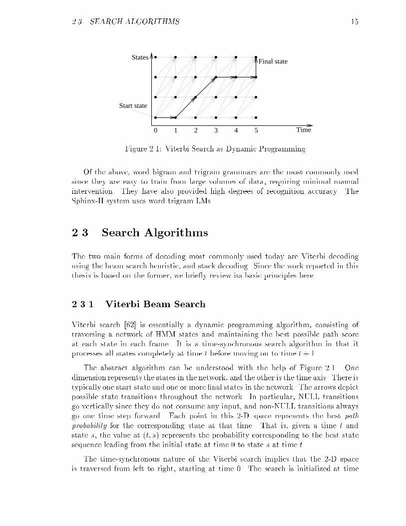
Figure 2.1: Viterbi Search as Dynamic Programming
Of the above, word bigram and trigram grammars are the most commonly usedsince they are easy to train from large volumes of data, requiring minimal manualintervention. They have also provided high degrees of recognition accuracy. TheSphinx-II system uses word trigram LMs.
2.3 Search Algorithms
The two main forms of decoding most commonly used today are Viterbi decodingusing the beam search heuristic, and stack decoding. Since the work reported in thisthesis is based on the former, we brie y review its basic principles here.
2.3.1 Viterbi Beam Search
Viterbi search [62] is essentially a dynamic programming algorithm, consisting oftraversing a network of HMM states and maintaining the best possible path scoreat each state in each frame. It is a time-synchronous search algorithm in that itprocesses all states completely at time t before moving on to time t+ 1.
The abstract algorithm can be understood with the help of Figure 2.1. Onedimension represents the states in the network, and the other is the time axis. There istypically one start state and one or more �nal states in the network. The arrows depictpossible state transitions throughout the network. In particular, NULL transitionsgo vertically since they do not consume any input, and non-NULL transitions alwaysgo one time step forward. Each point in this 2-D space represents the best pathprobability for the corresponding state at that time. That is, given a time t andstate s, the value at (t; s) represents the probability corresponding to the best statesequence leading from the initial state at time 0 to state s at time t.
The time-synchronous nature of the Viterbi search implies that the 2-D spaceis traversed from left to right, starting at time 0. The search is initialized at time
16 CHAPTER 2. BACKGROUND
t = 0 with the path probability at the start state set to 1, and at all other statesto 0. In each frame, the computation consists of evaluating all transitions betweenthe previous frame and the current frame, and then evaluating all NULL transitionswithin the current frame. For non-NULL transitions, the algorithm is summarizedby the following expression:
Pj(t) = maxi(Pi(t� 1) � aij � bi(t)); i� set of predecessor states of j (2.2)
where, Pj(t) is the path probability of state j at time t, aij is the static probabilityassociated with the transition from state i to j, and bi(t) is the output probabilityassociated with state i while consuming the input speech at t (see Section 2.1.2 andequation 2.1). It is straightforward to extend this formulation to include NULLtransitions that do not consume any input.
Thus, every state has a single best predecessor at each time instant. With somesimple bookkeeping to maintain this information, one can easily determine the beststate sequence for the entire search by starting at the �nal state at the end andfollowing the best predecessor at each step all the way back to the start state. Suchan example is shown by the bold arrows in Figure 2.1.
The complexity of Viterbi decoding is N2T (assuming each state can transitionto every state at each time step), where N is the total number of states and T is thetotal duration.
The application of Viterbi decoding to continuous speech recognition is straight-forward. Word HMMs are built by stringing together phonetic HMM models usingNULL transitions between the �nal state of one and the start state of the next. Inaddition, NULL transitions are added from the �nal state of each word to the initialstate of all words in the vocabulary, thus modelling continuous speech. Languagemodel (bigram) probabilities are associated with every one of these cross-word tran-sitions. Note that a system with a vocabulary of V words has V 2 possible cross-wordtransitions. All word HMMs are searched in parallel according to equation 2.2.
Since even a small to mediumvocabulary system consists of hundreds or thousandsof HMM states, the state-time matrix of Figure 2.1 quickly becomes too large andcostly to compute in its entirety. To keep the computation within manageable limits,only the most likely states are evaluated in each frame, according to the beam searchheuristic [37]. At the end of time t, the state with the highest path probability Pmax(t)is found. If any other state i has Pi(t) < Pmax(t) � B, where B is an appropriatelychosen threshold or beamwidth < 1, state i is excluded from consideration at timet+ 1. Only the ones within the beam are considered to be active.
The beam search heuristic reduces the average cost of search by orders of magni-tude in medium and large vocabulary systems. The combination of Viterbi decodingusing beam search heuristic is often simply referred to as Viterbi beam search.
2.4. RELATED WORK 17
2.4 Related Work
Some of the standard techniques in reducing the computational load of Viterbi searchfor large vocabulary continuous speech recognition have been the following:
� Narrowing the beamwidth for greater pruning. However, this is usually asso-ciated with an increase in error rate because of an increase in the number ofsearch errors: the correct word sometimes get pruned from the search path inthe bargain.
� Reducing the complexity of acoustic and language models. This approach worksto some extent, especially if it is followed by more detailed search in laterpasses. There is a tradeo� here, between the computational load of the �rstpass and subsequent ones. The use of detailed models in the �rst pass producescompact word lattices with low error rate that can be postprocessed e�ciently,but the �rst pass itself is computationally expensive. Its cost can be reduced ifsimpler models are employed, at the cost of an increase in lattice size needed toguarantee low lattice error rates.
Both the above techniques involve some tradeo� between recognition accuracy andspeed.
2.4.1 Tree Structured Lexicons
Organizing the HMMs to be searched as a phonetic tree instead of the at structureof independent linear HMM sequences for each word is probably the most often citedimprovement in search techniques in use currently. This structure is referred to astree-structured lexicon or lexical tree. If the pronunciations of two or more wordscontain the same n initial phonemes, they share a single sequence of n HMM modelsrepresenting that initial portion of their pronunciation. (In practice, most systemsuse triphones instead of just basephones, so we should really consider triphone pro-nunciation sequences. But the basic argument is the same.) Since the word-initialmodels in a non-tree structured Viterbi search are typically the majority of the totalnumber of active models, the reduction in computation is signi�cant.
The problem with a lexical tree occurs at word boundary transitions where bigramlanguage model probabilities are usually computed and applied. In the at (non-tree)Viterbi algorithm there is a transition from each word ending state (within the beam)to the beginning of every word in the vocabulary. Thus, there is a fan-in at theinitial state of every word, with di�erent bigram probabilities attached to every suchtransition. The Viterbi algorithm chooses the best incoming transition in each case.
However, with a lexical tree structure, several words may share the same root nodeof the tree. There can be a con ict between the best incoming cross-word transition
18 CHAPTER 2. BACKGROUND
for di�erent words that share the same root node. This problem has been usuallysolved by making copies of the lexical tree to resolve such con icts.
Approximate Bigram Trees
SRI [39] and CRIM [43] augment their lexical tree structure with a at copy of thelexicon that is activated for bigram transitions. All bigram transitions enter the atlexicon copy, while the backed o� unigram transitions enter the roots of the lexicaltree. SRI notes that relying on just unigrams more than doubles the word error rate.They show that using this scheme, the recognition speed is improved by a factor of2-3 for approximately the same accuracy. To gain further improvements in speed,they reduce the size of the bigram section by pruning the bigram language model invarious ways, which adds signi�cantly to the error rate.
However, it should be noted that the experimental set up is based on using discreteHMM acoustic models, with a baseline system word error rate (21.5%), which issigni�cantly worse than their best research system (10.3%) using bigrams, and alsoworse than most other research systems to begin with.
As we shall see in Chapter 3, bigram transitions constitute a signi�cant portion ofcross word transitions, which in turn are a dominant part of the search cost. Hence,the use of a at lexical structure for bigram transitions must continue to incur thiscost.
Replicated Bigram Trees
Ney and others [40, 3] have suggested creating copies of the lexical tree to handlebigram transitions. The leaf nodes at the �rst level (unigram) lexical tree have sec-ondary (bigram) trees hanging o� them for bigram transitions. The total size of thesecondary trees depends on the number of bigrams present in the grammar. Sec-ondary trees that represent the bigram followers of the most common function words,such as A, THE, IN, OF, etc. are usually large.
This scheme creates additional copies of words that did not exist in the original at structure. For example, in the conventional at lexicon (or in the auxiliary atlexicon copy of [39]), there is only one instance of each word. However, in thisproposed scheme the same word can appear in multiple secondary trees. Since theshort function words are recognized often (though spuriously), their bigram copiesare frequently active. They are also among the larger ones, as noted above. It isunclear how much overhead this adds to the system.
2.4. RELATED WORK 19
Dynamic Network Decoding
Cambridge University [44] designed a one-pass decoder that uses the lexical treestructure, with copies for cross-word transitions, but instantiates new copies at ev-ery transition, as necessary. Basically, the traditional re-entrant lexical structure isreplaced with a non-re-entrant structure. To prevent an explosion in memory spacerequirements, they reclaim HMM nodes as soon as they become inactive by fallingoutside the pruning beamwidth. Furthermore, the end points of multiple instances ofthe same word can be merged under the proper conditions, allowing just one instanceof the lexical tree to be propagated from the merged word ends, instead of separatelyand multiply from each. This system attained the highest recognition accuracy in theNov 1993 evaluations.
They report the performance under standard conditions|standard 1993 20K WallStreet Journal development test set decoded using the corresponding standard bi-gram/trigram language model using wide beamwidths as in the actual evaluations.
The number of active HMM models per frame in this scheme is actually higherthan the number in the baseline Sphinx-II system under similar test conditions (exceptthat Sphinx-II uses a di�erent lexicon and acoustic models). There are other factorsat work, but the dynamic instantiation of lexical trees certainly plays a part in thisincrease. The overhead for dynamically constructing the HMM network is reported tobe less than 20% of the total computational load. This is actually fairly high since thetime to decode a sentence on an HP735 platform is reported to be about 15 minuteson average.
2.4.2 Memory Size and Speed Improvements in Whisper
The CMU Sphinx-II system has been improved in many ways by Microsoft in pro-ducing the Whisper system [26]. They report that memory size has been reduced bya factor of 20 and speed improved by a factor of 5, compared to Sphinx-II under thesame accuracy constraints.
One of the schemes for memory reduction is the use of a context free grammar(CFG) in place of bigram or trigram grammars. CFGs are highly compact, canbe searched e�ciently, and can be relatively easily created for small tasks such ascommand and control applications involving a few hundred words. However, largevocabulary applications cannot be so rigidly constrained.
They also obtain an improvement of about 35% in the memory size of acousticmodels by using run length encoding for senone weighting coe�cients (Section 2.1.2).
They have also improved the speed performance of Whisper through a Rich GetRicher (RGR) heuristic for deciding which phones should be evaluated in detail, usingtriphone states, and which should fall back on context independent phone states.
20 CHAPTER 2. BACKGROUND
RGR works as follows: Let Pp(t) be the best path probability of any state belongingto basephone p at time t, Pmax(t) the best path probability over all states at t, andbp(t+1) the output probability of the context-independent model for p at time t+1.Then, the context-dependent states for phone p are evaluated at frame t+ 1 i�:
a � Pp(t) + bp(t+ 1) > Pmax(t)�K
where, a andK are empirically determined constants. Otherwise, context-independentoutput probabilities are used for those states. (All probabilities are computed inlog-space. Hence the addition operations really represent multiplications in normalprobability space.)
Using this heuristic, they report an 80% reduction in the number of context de-pendent states for which output probabilities are computed, with no loss of accuracy.If the parameters a and K are tightened to reduce the number of context-dependentstates evaluated by 95%, there is a 15% relative loss of accuracy. (The baseline testconditions have not be speci�ed for these experiments.)
2.4.3 Search Pruning Using Posterior Phone Probabilities
In [56], Renals and Hochberg describe a method of deactivating certain phones duringsearch to achieve higher recognition speed. The method is incorporated into a fastmatch pass that produces words and posterior probabilities for their noway stackdecoder. The fast match step uses HMM base phone models, the states of whichare modelled by neural networks that directory estimate phone posterior probabil-ities instead of the usual likelihoods; i.e., they estimate P (phonejdata), instead ofP (datajphone). Using the posterior phone probability information, one can identifythe less likely active phones at any given time and prune the search accordingly.
This is a potentially powerful and easy pruning technique when the posterior phoneprobabilities are available. Stack decoders can particularly gain if the fast match stepcan be made to limit the number of candidate words emitted while extending apartial hypothesis. In their noway implementation, a speedup of about an order ofmagnitude is observed on a 20K vocabulary task (from about 150x real time to about15x real time) on an HP735 workstation. They do not report the reduction in thenumber of active HMMs as a result of this pruning.
2.4.4 Lower Complexity Viterbi Algorithm
A new approach to the Viterbi algorithm, speci�cally applicable to speech recognition,is described by Patel in [49]. It is aimed at reducing the cost of the large numberof cross-word transitions and has an expected complexity of N
pNT , instead of N2T
(Section 2.3.1). The algorithm depends on ordering the exit path probabilities and
2.5. SUMMARY 21
transition bigram probabilities, and �nding a threshold such that most transitionscan be eliminated from consideration.
The authors indicate that the algorithm o�ers better performance if every wordhas bigram transitions to the entire vocabulary. However, this is not the case withlarge vocabulary systems. Nevertheless, it is worth exploring this technique furtherfor its practical applicability.
2.5 Summary
In this chapter we have covered the basic modelling principles and search techniquescommonly used in speech recognition today. We have also brie y reviewed a numberof systems and techniques used to improve their speed and memory requirements. Oneof the main themes running through this work is that virtually none of the practicalimplementations have been formally evaluated with respect to the research systemson well established test sets under widely used test conditions, or with respect to oneanother.
In the rest of this thesis, we evaluate the baseline Sphinx-II system under normalevaluation conditions and use the results for comparison with our other experiments.

Chapter 3
The Sphinx-II Baseline System
As mentioned in the previous chapters, there is relatively little published work onthe performance of speech recognition systems, measured along the dimensions ofrecognition accuracy, speed and resource utilization. The purpose of this chapter isto establish a comprehensive account of the performance of a baseline system thathas been considered a premier representative of its kind, with which we can makemeaningful comparisons of the research reported in this thesis. For this purpose, wehave chosen the Sphinx-II speech recognition system1 at Carnegie Mellon that hasbeen used extensively in speech research and the yearly ARPA evaluations. Variousaspects of this baseline system and its precursors have been reported in the literature,notably in [32, 33, 35, 28, 1, 2]. Most of these concentrate on the modelling aspectsof the system|acoustic, grammatical or lexical|and their e�ect on recognition ac-curacy. In this chapter we focus on obtaining a comprehensive set of performancecharacteristics for this system.
The baseline Sphinx-II recognition system uses semi-continuous or tied-mixturehidden Markov models (HMMs) for the acoustic models [52, 27, 12] and word bigramor trigram backo� language models (see Sections 2.1 and 2.2). It is a 3-pass decoderstructured as follows:
1. Time synchronous Viterbi beam search [52, 62, 37] in the forward direction. It isa complete search of the full vocabulary, using semi-continuous acoustic models,a bigram or trigram language model, and cross-word triphone modelling duringthe search. The result of this search is a single recognition hypothesis, as well asa word lattice that contains all the words that were recognized during the search.The lattice includes word segmentation and scores information. One of the keyfeatures of this lattice is that for each word occurrence, several successive endtimes are identi�ed along with their scores, whereas very often only the singlemost likely begin time is identi�ed. Scores for alternative begin times are usually
1The Sphinx-II decoder reported in this section is known internally as FBS6.
22
23
not available.
2. Time synchronous Viterbi beam search in the backward direction. This searchis restricted to the words identi�ed in the forward pass and is very fast. Likethe �rst pass, it produces a word lattice with word segmentations and scores.However, this time several alternative begin times are identi�ed while typicallyonly one end time is available. In addition, the Viterbi search also producesthe best path score from any point in the utterance to the end of the utterance,which is used in the third pass.
3. An A* or stack search using the word segmentations and scores produced by theforward and backward Viterbi passes above. It produces an N-best list [59] ofalternative hypotheses as its output, as described brie y in Section 1.2. Thereis no acoustic rescoring in this pass. However, any arbitrary language modelcan be applied in creating the N-best list. In this thesis, we will restrict ourdiscussion to word trigram language models.
The reason for the existence of the backward and A* passes, even though the�rst pass produces a usable recognition result, is the following. One limitation of theforward Viterbi search in the �rst pass is that it is hard to employ anything moresophisticated than a simple bigram or similar grammar. Although a trigram grammaris used in the forward pass, it is not a complete trigram search (see Section 3.2.2).Stack decoding, a variant of the A* search algorithm2 [42], is more appropriate foruse with such grammars which lead to greater recognition accuracy. This algorithmmaintains a stack of several possible partial decodings (i.e, word sequence hypotheses)which are expanded in a best-�rst manner [9, 2, 50]. Since each partial hypothesisis a linear word sequence, any arbitrary language model can be applied to it. Stackdecoding also allows the decoder to output several most likely N-best hypothesesrather than just the single best one. These multiple hypotheses can be postprocessedwith even more detailed models. The need for the backward pass in the baselinesystem has been mentioned above.
In this chapter we review the details of the baseline system needed for under-standing the performance characteristics. In order to keep this discussion fairly self-contained, we �rst review the various knowledge source models in Section 3.1. Someof the background material in Sections 2.1, 2.2, and 2.3 is also relevant. This is fol-lowed by a discussion of the forward pass Viterbi beam search in Section 3.2, and thebackward and A* searches in Section 3.3. The performance of this system on sev-eral widely used test sets from the ARPA evaluations is described in Section 3.4. Itincludes recognition accuracy, various statistics related to search speed, and memoryusage. We �nally conclude with some �nal remarks in Section 3.5.
2We will often use the terms stack decoding and A* search interchangeably.
24 CHAPTER 3. THE SPHINX-II BASELINE SYSTEM
Pre−emphasis Filter
H(z) = 1−0.97z−1
25.6msecHamming Window
10msec intervals
12 mel freq. coeff.+
power coeff.
power andcepstral normalization
cepstrum−vectorpower
cepstrum cepstrum power, power,
25.6ms
10ms
16KHz, 16−bit linear samples
sentence−based power −= max(power) over sentencecepstrum −= mean(cepstrum) over sentence
100 cepstral frames/sec
4 feature streams at 100 frames/sec.
Figure 3.1: Sphinx-II Signal Processing Front End.
3.1 Knowledge Sources
This section brie y describes the various knowledge sources or models and the speechsignal processing front-end used in Sphinx-II. In addition to the acoustic modelsand pronunciation lexicon described below, Sphinx-II uses word bigram and trigramgrammars. These have been discussed in Section 2.2.
3.1.1 Acoustic Model
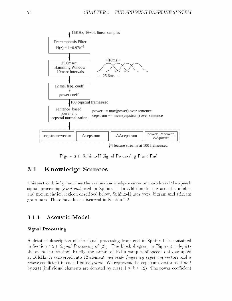
Signal Processing
A detailed description of the signal processing front end in Sphinx-II is containedin Section 4.2.1 Signal Processing of [27]. The block diagram in Figure 3.1 depictsthe overall processing. Brie y, the stream of 16-bit samples of speech data, sampledat 16KHz, is converted into 12-element mel scale frequency cepstrum vectors and apower coe�cient in each 10msec frame. We represent the cepstrum vector at time tby x(t) (individual elements are denoted by xk(t); 1 � k � 12). The power coe�cient
3.1. KNOWLEDGE SOURCES 25
0 1 2 3 4
Initial State Final State(Non−emitting)
Figure 3.2: Sphinx-II HMM Topology: 5-State Bakis Model.
is simply x0(t). This cepstrum vector and power streams are �rst normalized, andfour feature vectors are derived in each frame by computing the �rst and second orderdi�erences in time:
x(t) = normalized cepstrum vector�x(t) = x(t+ 2)� x(t� 2); �lx(t) = x(t+ 4) � x(t� 4)��x(t) = �x(t+ 1) ��x(t� 1)x0(t) = x0(t);
�x0(t) = x0(t+ 2)� x0(t� 2);��x0(t) = �x0(t+ 1) ��x0(t� 1)
where the commas denote concatenation. Thus, in every frame we obtain four featurevectors of 12, 24, 12, and 3 elements, respectively. These, ultimately, are the inputto the speech recognition system.
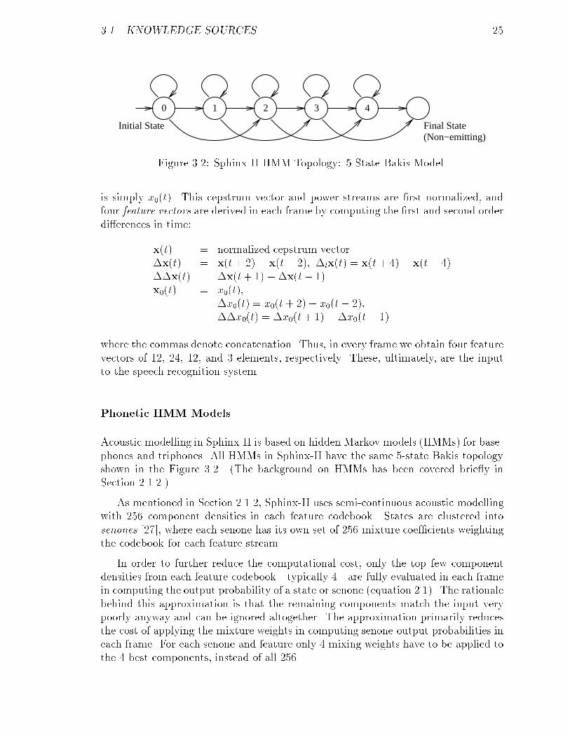
Phonetic HMM Models
Acoustic modelling in Sphinx-II is based on hidden Markov models (HMMs) for base-phones and triphones. All HMMs in Sphinx-II have the same 5-state Bakis topologyshown in the Figure 3.2. (The background on HMMs has been covered brie y inSection 2.1.2.)
As mentioned in Section 2.1.2, Sphinx-II uses semi-continuous acoustic modellingwith 256 component densities in each feature codebook. States are clustered intosenones [27], where each senone has its own set of 256 mixture coe�cients weightingthe codebook for each feature stream.
In order to further reduce the computational cost, only the top few componentdensities from each feature codebook|typically 4|are fully evaluated in each framein computing the output probability of a state or senone (equation 2.1). The rationalebehind this approximation is that the remaining components match the input verypoorly anyway and can be ignored altogether. The approximation primarily reducesthe cost of applying the mixture weights in computing senone output probabilities ineach frame. For each senone and feature only 4 mixing weights have to be applied tothe 4 best components, instead of all 256.
26 CHAPTER 3. THE SPHINX-II BASELINE SYSTEM
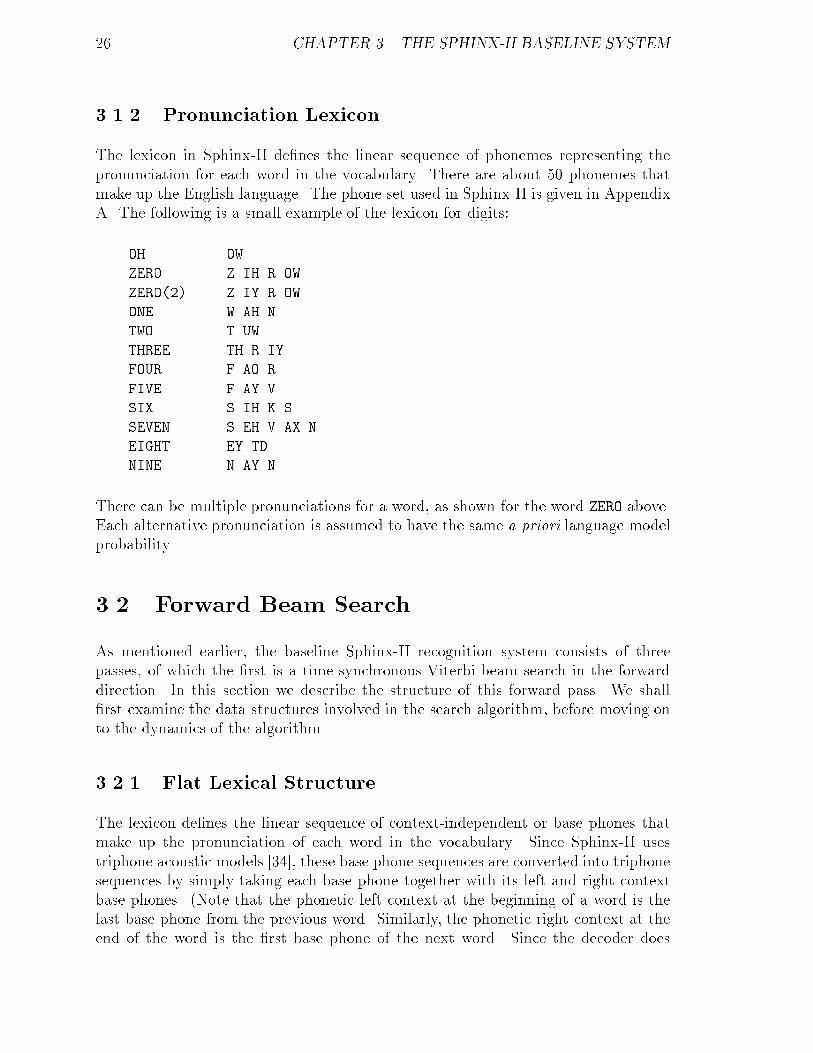
3.1.2 Pronunciation Lexicon
The lexicon in Sphinx-II de�nes the linear sequence of phonemes representing thepronunciation for each word in the vocabulary. There are about 50 phonemes thatmake up the English language. The phone set used in Sphinx-II is given in AppendixA. The following is a small example of the lexicon for digits:
OH OW
ZERO Z IH R OW
ZERO(2) Z IY R OW
ONE W AH N
TWO T UW
THREE TH R IY
FOUR F AO R
FIVE F AY V
SIX S IH K S
SEVEN S EH V AX N
EIGHT EY TD
NINE N AY N
There can be multiple pronunciations for a word, as shown for the word ZERO above.Each alternative pronunciation is assumed to have the same a priori language modelprobability.
3.2 Forward Beam Search
As mentioned earlier, the baseline Sphinx-II recognition system consists of threepasses, of which the �rst is a time-synchronous Viterbi beam search in the forwarddirection. In this section we describe the structure of this forward pass. We shall�rst examine the data structures involved in the search algorithm, before moving onto the dynamics of the algorithm.
3.2.1 Flat Lexical Structure
The lexicon de�nes the linear sequence of context-independent or base phones thatmake up the pronunciation of each word in the vocabulary. Since Sphinx-II usestriphone acoustic models [34], these base phone sequences are converted into triphonesequences by simply taking each base phone together with its left and right contextbase phones. (Note that the phonetic left context at the beginning of a word is thelast base phone from the previous word. Similarly, the phonetic right context at theend of the word is the �rst base phone of the next word. Since the decoder does
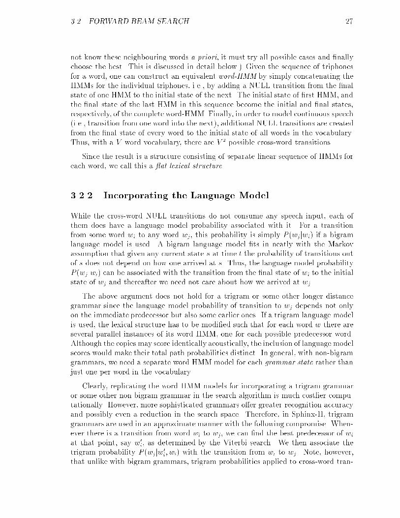
3.2. FORWARD BEAM SEARCH 27
not know these neighbouring words a priori, it must try all possible cases and �nallychoose the best. This is discussed in detail below.) Given the sequence of triphonesfor a word, one can construct an equivalent word-HMM by simply concatenating theHMMs for the individual triphones, i.e., by adding a NULL transition from the �nalstate of one HMM to the initial state of the next. The initial state of �rst HMM, andthe �nal state of the last HMM in this sequence become the initial and �nal states,respectively, of the complete word-HMM. Finally, in order to model continuous speech(i.e., transition from one word into the next), additional NULL transitions are createdfrom the �nal state of every word to the initial state of all words in the vocabulary.Thus, with a V word vocabulary, there are V 2 possible cross-word transitions.
Since the result is a structure consisting of separate linear sequence of HMMs foreach word, we call this a at lexical structure.
3.2.2 Incorporating the Language Model
While the cross-word NULL transitions do not consume any speech input, each ofthem does have a language model probability associated with it. For a transitionfrom some word wi to any word wj, this probability is simply P (wjjwi) if a bigramlanguage model is used. A bigram language model �ts in neatly with the Markovassumption that given any current state s at time t the probability of transitions outof s does not depend on how one arrived at s. Thus, the language model probabilityP (wjjwi) can be associated with the transition from the �nal state of wi to the initialstate of wj and thereafter we need not care about how we arrived at wj.
The above argument does not hold for a trigram or some other longer distancegrammar since the language model probability of transition to wj depends not onlyon the immediate predecessor but also some earlier ones. If a trigram language modelis used, the lexical structure has to be modi�ed such that for each word w there areseveral parallel instances of its word HMM, one for each possible predecessor word.Although the copies may score identically acoustically, the inclusion of language modelscores would make their total path probabilities distinct. In general, with non-bigramgrammars, we need a separate word HMM model for each grammar state rather thanjust one per word in the vocabulary.
Clearly, replicating the word HMM models for incorporating a trigram grammaror some other non-bigram grammar in the search algorithm is much costlier compu-tationally. However, more sophisticated grammars o�er greater recognition accuracyand possibly even a reduction in the search space. Therefore, in Sphinx-II, trigramgrammars are used in an approximate manner with the following compromise. When-ever there is a transition from word wi to wj, we can �nd the best predecessor of wi
at that point, say w0
i, as determined by the Viterbi search. We then associate thetrigram probability P (wjjw0
i; wi) with the transition from wi to wj. Note, however,that unlike with bigram grammars, trigram probabilities applied to cross-word tran-
28 CHAPTER 3. THE SPHINX-II BASELINE SYSTEM
sitions in this approximate fashion have to be determined dynamically, depending onthe best predecessor for each transition at the time in question.
Using a trigram grammar in an approximate manner as described above has thefollowing advantages:
� It avoid any replication of the lexical word-HMM structures and associatedincrease in computational load.
� In terms of accuracy, it is much better than using a bigram model and is close tothat of a complete trigram search. We infer this from the fact that the accuracyof the results from the �nal A* pass, which uses the trigram grammar correctly,and also has the bene�t of additional word segmentations to choose from, isrelatively only about 5% better (see Section 3.4.2).
� A trigram grammar applied in this approximate manner is empirically observedto search fewer word-HMMs compared to a bigram grammar, thus leading to aslight improvement in the recognition speed. The reduction in search is a resultof sharper pruning o�ered by the trigram grammar.
3.2.3 Cross-Word Triphone Modeling
It is advantageous to use cross-word triphone models (as opposed to ignoring cross-word phonetic contexts) for continuous speech recognition where word boundariesare unclear to begin with and there are very strong co-articulation e�ects. Usingcross-word triphone models we not only obtain better accuracy, but also greater com-putational e�ciency, at the cost of an increase in the total size of acoustic models.The sharper models provided by triphones, compared to diphones and monophones,leads to greater pruning e�ciency and a reduction in computation. However, us-ing cross-word triphone models in the Viterbi search algorithm is not without itscomplications.
Right Context
The phonetic right context for the last triphone position in a word is the �rst basephone of the next word. In time-synchronous Viterbi search, there is no way to knowthe next word in advance. In any case, whatever decoding algorithm is used, therecan be several potential successor words to any given word wi at any given time.Therefore, the last triphone position for each word has to be modelled by a parallelset of triphone models, one for each possible phonetic right context. In other words, ifthere are k basephones p1; p2; : : : ; pk in the system, we have k parallel triphone HMMmodels hp1; hp2; : : : ; hpk representing the �nal triphone position for wi. A cross-wordtransition from wi to another word wj , whose �rst base phone is p is represented by

3.2. FORWARD BEAM SEARCH 29
p
p
p
p
1
2
3
k
p
wi
Word wj
HMM network for word
last phone position fordifferent phoneticright contexts
, first basephone = p
Cross−word NULL transition
Right contextbasephone
Parallel set of HMMs in
Figure 3.3: Cross-word Triphone Modelling at Word Ends in Sphinx-II.
a NULL arc from hp to the initial state of wj. Figure 3.3 illustrates this concept ofright context fanout at the end of each word wi in Sphinx-II.
This solution, at �rst glance, appears to force a large increase in the total numberof triphone HMMs that may be searched. In the place of the single last positiontriphone for each word, we now have one triphone model for each possible phoneticright context, which is typically around 50 in number. In practice, we almost neverencounter this apparent explosion in computational load, for the following reasons:
� The dynamic number of rightmost triphones actually evaluated in practice ismuch smaller than the static number because the beam search heuristic prunesmost of the words away by the time their last phone has been reached. This isby far the largest source of e�ciency, even with the right context fanout.
� The set of phonetic right contexts actually modelled can be restricted to justthose found in the input vocabulary; i.e., to the set of �rst base phones of allthe words in the vocabulary.
Moreover, Sphinx-II uses state clustering into senones, where several statesshare the same output distribution modelled by a senone. Therefore, the parallelset of models at the end of any given word are not all unique. By removingduplicates, the fanout can be further reduced. In Sphinx-II, these two factorstogether reduce the right context fanout by about 70% on average.
� The increase is number of rightmost triphones is partly o�set by the reductionin computation a�orded by the sharper triphone models.
30 CHAPTER 3. THE SPHINX-II BASELINE SYSTEM
Left Context
The phonetic left context for the �rst phone position in a word is the last basephone from the previous word. During decoding, there is no unique such predecessorword. In any given frame t, there may be transitions to a word wj from a numberof candidates wi1 ; wi2; : : : The Viterbi algorithm chooses the best possible transitioninto wj . Let us say the winning predecessor is wik . Thus, the last base phone of wik
becomes the phonetic left context for wj. However, this is in frame t. In the nextframe, there may be an entirely di�erent winner that results in a di�erent left contextbase phone. Since the real best predecessor is not determined until the end of theViterbi decoding, all such possible paths have to be pursued in parallel.
As with right context cross-word triphone modelling, this problem also can solvedby using a parallel set of triphone models for the �rst phone position of each word|aseparate triphone for each possible phonetic left context. However, unlike the word-ending phone position which is heavily pruned by the beam search heuristic, the word-initial position is extensively searched. Most of the word-initial triphone models arealive every frame. In fact, as we shall see later in Section 3.4, they account for morethan 60% of all triphone models evaluated in the case of large-vocabulary recognition.A left context fanout of even a small factor of 2 or 3 would substantially slow downthe system.
The solution used in the Sphinx-II baseline system is to collapse the left contextfanout into a single 5-state HMM with dynamic triphone mapping as follows. Asdescribed above, at any given frame there may be several possible transitions fromwords wi1; wi2 ; : : : into wj . According to the Viterbi algorithm, the transition withthe best incoming score wins. Let the winning predecessor be wik . Then the initialstate of wj also dynamically inherits the last base phone of wik as its left context.When the output probability of the initial state of wj has to be evaluated in the nextframe, its parent triphone identity is �rst determined dynamically from the inheritedleft context basephone. Furthermore, this dynamically determined triphone identityis also propagated by the Viterbi algorithm, as the path probability is propagatedfrom state to state. This ensures that any complete path through the initial triphoneposition of wj is scored consistently using a single triphone HMM model.
Figure 3.4 illustrates this process with an example, going through a sequence of4 frames. It contains a snapshot of a word-initial HMM model at the end of eachframe. Arcs in bold indicate the winning transitions to each state of the HMM inthis example. HMM states are annotated with the left context basephone inheriteddynamically through time. As we can see in the example, di�erent states can have dif-ferent phonetic left contexts associated with them, but a single Viterbi path throughthe HMM is evaluated with the same context. This can be veri�ed by backtrackingfrom the �nal state backward in time.
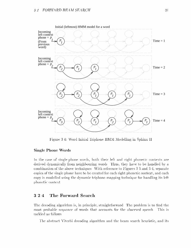
3.2. FORWARD BEAM SEARCH 31
p1
p2
p3
p1
p1
p1
p1
p1
p2
p2
p1
p1
p2
p2
previous
p1 Time = 1
Time = 2
Time = 3
Time = 4
left contextIncoming
phone =
pleft contextIncoming
(From
word)
pleft contextIncoming
2
3
Initial (leftmost) HMM model for a word
p1
phone =
phone =
Figure 3.4: Word Initial Triphone HMM Modelling in Sphinx-II.
Single Phone Words
In the case of single-phone words, both their left and right phonetic contexts arederived dynamically from neighbouring words. Thus, they have to be handled by acombination of the above techniques. With reference to Figures 3.3 and 3.4, separatecopies of the single phone have to be created for each right phonetic context, and eachcopy is modelled using the dynamic triphone mapping technique for handling its leftphonetic context.
3.2.4 The Forward Search
The decoding algorithm is, in principle, straightforward. The problem is to �nd themost probable sequence of words that accounts for the observed speech. This istackled as follows.
The abstract Viterbi decoding algorithm and the beam search heuristic, and its
32 CHAPTER 3. THE SPHINX-II BASELINE SYSTEM
application to speech decoding have been explained in Section 2.3.1. In Sphinx-II,there are two distinguished words, <s> and </s> , depicting the beginning and endingsilence in any utterance. The input speech is expected to begin at the initial state of<s> and end in the �nal state of </s> .
We can now described the forward Viterbi beam search implementation in Sphinx-II. It is explained with the help of fragments of pseudo-code. It is necessary tounderstand the forward pass at this level in order to follow the subsequent discussionon performance analysis and the breakdown of computation among di�erent modules.
Search Outline
Before we go into the details of the search algorithm, we introduce some terminology.A state j of an HMM model m in the at lexical search space has the followingattributes:
� A path score at time t, Pmj (t), that indicates the probability corresponding to
the best state sequence leading from the initial state of <s> at time 0 to thisstate at time t, while consuming the input speech until t.
� A history information at time t, Hmj (t), that allows us to trace back the best
preceding word history leading to this state at t. (As we shall see later, this isa pointer to the word lattice entry containing the best predecessor word.)
� The senone output probability, bmj (t), for this state at time t (see Section 2.1.2).If m belongs to the �rst position in a word, the senone identity for state j isdetermined dynamically from the inherited phonetic left context (Section 3.2.3).
At the beginning of the decoding of an utterance, the search process is initializedby setting the path probability of the start state of the distinguished word <s> to 1.All other states are initialized with a path score of 0. Also, an active HMM list thatidenti�es the set of active HMMs in the current frame is initialized with this �rstHMM for <s> . From then on, the processing of each frame of speech, given the inputfeature vector for that frame, is outlined by the pseudo-code in Figure 3.5.
We consider some of the functions de�ned in Figure 3.5 in a little more detail be-low. Certain aspects, such as pruning out HMMs that fall below the beam threshold,have been omitted for the sake of simplicity.
VQ: VQ stands for vector quantization. In this function, the Gaussian densitiesthat make up each feature codebook are evaluated at the input feature vectors. Inother words, we compute the Mahalanobis distance of the input feature vector fromthe mean of each Gaussian density function. (This corresponds to evaluating N in
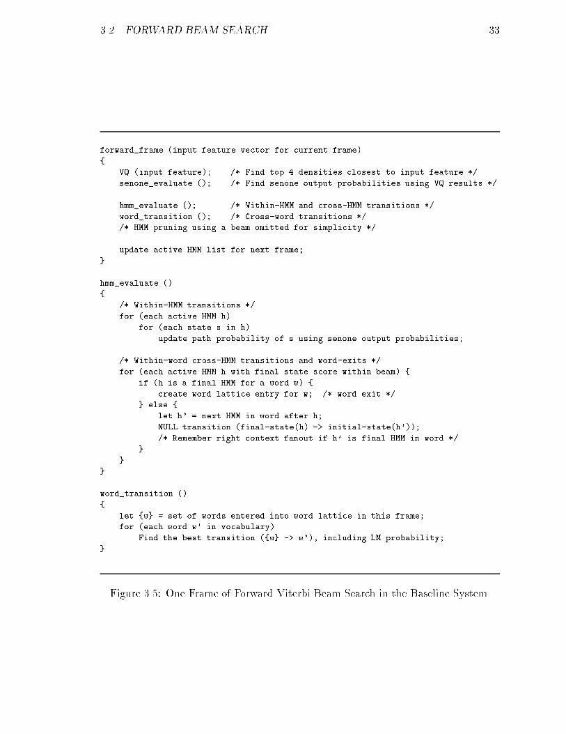
3.2. FORWARD BEAM SEARCH 33
forward_frame (input feature vector for current frame)
{
VQ (input feature); /* Find top 4 densities closest to input feature */
senone_evaluate (); /* Find senone output probabilities using VQ results */
hmm_evaluate (); /* Within-HMM and cross-HMM transitions */
word_transition (); /* Cross-word transitions */
/* HMM pruning using a beam omitted for simplicity */
update active HMM list for next frame;
}
hmm_evaluate ()
{
/* Within-HMM transitions */
for (each active HMM h)
for (each state s in h)
update path probability of s using senone output probabilities;
/* Within-word cross-HMM transitions and word-exits */
for (each active HMM h with final state score within beam) {
if (h is a final HMM for a word w) {
create word lattice entry for w; /* word exit */
} else {
let h' = next HMM in word after h;
NULL transition (final-state(h) -> initial-state(h'));
/* Remember right context fanout if h' is final HMM in word */
}
}
}
word_transition ()
{
let {w} = set of words entered into word lattice in this frame;
for (each word w' in vocabulary)
Find the best transition ({w} -> w'), including LM probability;
}
Figure 3.5: One Frame of Forward Viterbi Beam Search in the Baseline System.

34 CHAPTER 3. THE SPHINX-II BASELINE SYSTEM
equation 2.1.) Only the top 4 densities are fully evaluated and used further, since therest typically contribute very little to the senone output probability.
Since all senones share a single codebook per feature stream in the Sphinx-IIsemi-continuous model, the VQ step does not have to be repeated for each senone.
Senone Evaluation: (Function senone_evaluate.) In this function, we computethe output probability for each senone in the current frame as a weighted sum ofthe top 4 density values in the frame. There are 4 feature streams in Sphinx-II. Theweighting is done independently on each stream and the �nal result is the product ofthe four weighted values. (See Sections 3.1.1 and 2.1.2.)
HMM Evaluation: (Function hmm_evaluate.) This step includes two cases:
� Within-HMM transitions: For each active HMM model m the path score ofeach state j in m is updated according to:
Pmj (t) = max
i(Pm
i (t� 1) � bmi (t) � amij ) (3.1)
where, t indicates the current frame, i ranges over all states of m, and amijis a static probability for the arc from i to j in m. (See also Section 2.1.2.)Furthermore, the history pointer Hm
j (t), and the dynamic phonetic left contextif applicable, are propagated to j from the state i that maximizes expression3.1.
� Within-word cross-HMM transitions and Word Exits: A cross-HMM NULLtransition within a word from HMMm1 to m2 causes the path score and historyinformation to be propagated from the �nal state of m1 to the start state of m2
if it results in a better path score at the start state of m2.
Words whose �nal states have a score within the allowed threshold representpotential word recognitions in the current frame. There can be several suchwords in any given frame. All of them are entered in a word lattice along withthe path score and history information from the �nal state. The right contextfanout at the end of each word actually results in several entries for each word,one for each possible phonetic right context.
Cross-Word Transition: (Function word_transition.) In principle, this stepattempts all possible cross-word transitions from the set of words exited to all wordsin the vocabulary, computing the language model probability in each case. If n wordsreached their �nal state in the current frame, and there are V words in the vocabulary,a total of nV transitions are possible. This is an enormous number. However, not alltransitions have explicit trigram or even bigram probabilities in the language model.
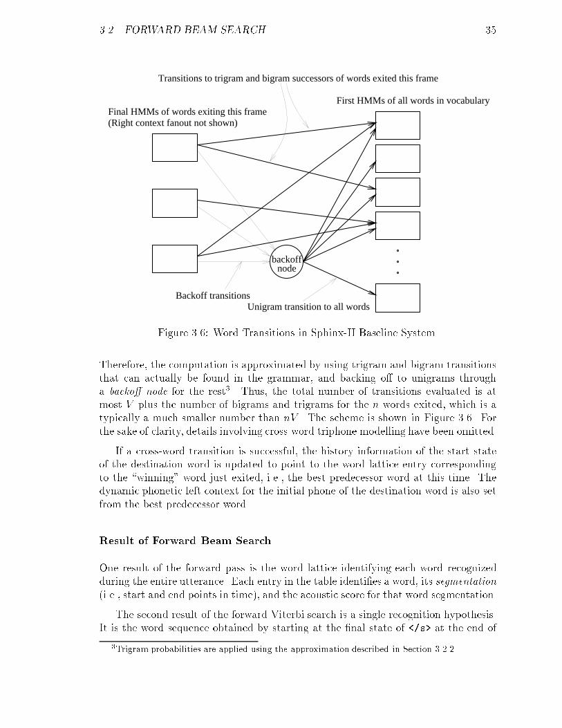
3.2. FORWARD BEAM SEARCH 35
Final HMMs of words exiting this frameFirst HMMs of all words in vocabulary
(Right context fanout not shown)
Backoff transitions
backoffnode
Unigram transition to all words
Transitions to trigram and bigram successors of words exited this frame
Figure 3.6: Word Transitions in Sphinx-II Baseline System.
Therefore, the computation is approximated by using trigram and bigram transitionsthat can actually be found in the grammar, and backing o� to unigrams througha backo� node for the rest3. Thus, the total number of transitions evaluated is atmost V plus the number of bigrams and trigrams for the n words exited, which is atypically a much smaller number than nV . The scheme is shown in Figure 3.6. Forthe sake of clarity, details involving cross-word triphone modelling have been omitted.
If a cross-word transition is successful, the history information of the start stateof the destination word is updated to point to the word lattice entry correspondingto the \winning" word just exited, i.e., the best predecessor word at this time. Thedynamic phonetic left context for the initial phone of the destination word is also setfrom the best predecessor word.
Result of Forward Beam Search
One result of the forward pass is the word lattice identifying each word recognizedduring the entire utterance. Each entry in the table identi�es a word, its segmentation(i.e., start and end points in time), and the acoustic score for that word segmentation.
The second result of the forward Viterbi search is a single recognition hypothesis.It is the word sequence obtained by starting at the �nal state of </s> at the end of
3Trigram probabilities are applied using the approximation described in Section 3.2.2.
36 CHAPTER 3. THE SPHINX-II BASELINE SYSTEM
the utterance and backtracking to the beginning, by following the history pointers inthe word lattice.
3.3 Backward and A* Search
As mentioned earlier, the A* or stack search is capable of exactly using more so-phisticated language models than bigram grammars, thus o�ering higher recognitionaccuracy. It maintains a sorted stack of partial hypotheses which are expanded in abest-�rst manner, one word length at a time. There are two main issues with thisalgorithm:
� To prevent an exponential explosion in the search space, the stack decodingalgorithm must expand each partial hypothesis only by a limited set of themost likely candidate words that may follow that partial hypothesis.
� The A* algorithm is not time synchronous. Speci�cally, each partial hypothesesin the sorted stack can account for a di�erent initial segment of the input speech.This makes it hard to compare the path probabilities of the entries in the stack.
It has been shown in [42] that the second issue can be solved by attaching a heuris-tic score with every partial hypothesis H that accounts for the remaining portion ofthe speech not included in H. By \�lling out" every partial hypothesis to the fullutterance length in this way, the entries in the stack can be compared to one another,and expanded in a best-�rst manner. As long as the heuristic score attached to anypartial hypothesis H is an upper bound on the score of the best possible completerecognition achievable from H, the A* algorithm is guaranteed to produce the correctresults.
The backward pass in the Sphinx-II baseline system provides an approximation tothe heuristic score needed by the A* algorithm. Since it is a time-synchronous Viterbisearch, run in the backward direction from the end of the utterance, the path scoreat any state corresponds to the best state sequence between it and the utterance end.Hence it serves as the desired upper bound. It is an approximation since the pathscore uses bigram probabilities and not the exact grammar that the A* search uses.
The backward pass also produces a word lattice, similar to the forward Viterbisearch. The A* search is constrained to search only the words in the two lattices, andis relatively fast.
The word lattice produced by the backward pass has another desirable property.We noted at the beginning of this chapter that for each word occurrence in the forwardpass word lattice, several successive end times are identi�ed along with their scores,whereas very often only the single most likely begin time is identi�ed. The backwardpass word lattice produces the complementary result: several beginning times are
3.3. BACKWARD AND A* SEARCH 37
identi�ed for a given word occurrence, while usually only the single most likely endtime is available. The two lattices can be combined to obtain acoustic probabilitiesfor a wider range of word beginning and ending times, which improves the recognitionaccuracy.
In the following subsections, we brie y describe the backward Viterbi pass andthe A* algorithm used in the Sphinx-II baseline system.
3.3.1 Backward Viterbi Search
The backward Viterbi search is essentially identical to the forward search, except thatit is completely reversed in time. The main di�erences are listed below:
� The input speech is processed in reverse.
� It is constrained to search only the words in the word lattice from the forwardpass. Speci�cally, at any time t, cross-word transitions are restricted to wordsthat exited at t in the forward pass, as determined by the latter's word lattice.
� All HMM transitions, as well as cross-HMM and cross-word NULL transitionsare reversed with respect to the forward pass.
� Cross word triphone modelling is performed using left-context fanout and dy-namic triphone mapping for right contexts.
� Only the bigram probabilities are used. Therefore, the Viterbi path score fromany point in the utterance up to the end is only an approximation to the upperbounds desired by the A* search.
The result of the backward Viterbi search is also a word lattice like that from theforward pass. It is rooted at </s> that ends in the �nal frame of the utterance, andgrowing backward in time. The backward pass identi�es several beginning times for aword, but typically only one ending time. Acoustic scores for each word segmentationare available in the backward pass word lattice.
3.3.2 A* Search
The A* search algorithm is described in [42]. It works by maintaining an ordered stackor list of partial hypotheses, sorted in descending order of likelihood. Hypotheses areword sequences and may be of di�erent lengths, accounting for di�erent lengths ofinput speed. Figure 3.7 outlines the basic stack decoding algorithm for �nding N -besthypotheses.
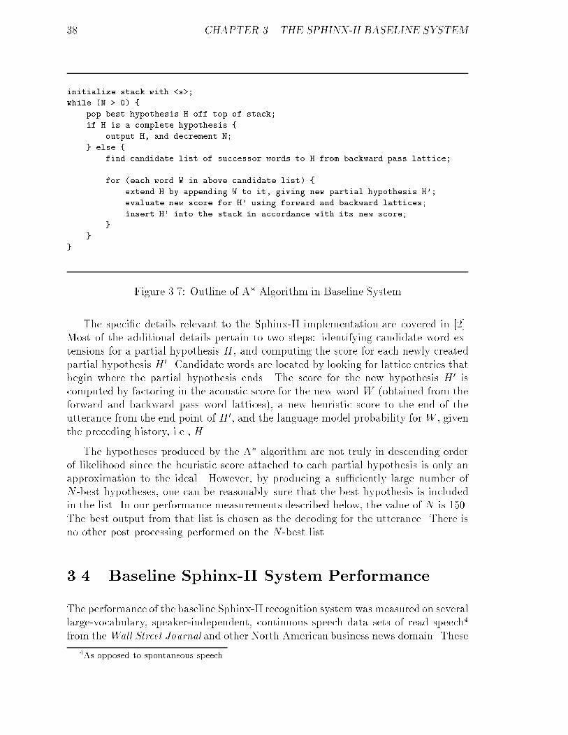
38 CHAPTER 3. THE SPHINX-II BASELINE SYSTEM
initialize stack with <s>;
while (N > 0) {
pop best hypothesis H off top of stack;
if H is a complete hypothesis {
output H, and decrement N;
} else {
find candidate list of successor words to H from backward pass lattice;
for (each word W in above candidate list) {
extend H by appending W to it, giving new partial hypothesis H';
evaluate new score for H' using forward and backward lattices;
insert H' into the stack in accordance with its new score;
}
}
}
Figure 3.7: Outline of A* Algorithm in Baseline System
The speci�c details relevant to the Sphinx-II implementation are covered in [2].Most of the additional details pertain to two steps: identifying candidate word ex-tensions for a partial hypothesis H, and computing the score for each newly createdpartial hypothesis H 0. Candidate words are located by looking for lattice entries thatbegin where the partial hypothesis ends. The score for the new hypothesis H 0 iscomputed by factoring in the acoustic score for the new word W (obtained from theforward and backward pass word lattices), a new heuristic score to the end of theutterance from the end point of H 0, and the language model probability for W , giventhe preceding history, i.e., H.
The hypotheses produced by the A* algorithm are not truly in descending orderof likelihood since the heuristic score attached to each partial hypothesis is only anapproximation to the ideal. However, by producing a su�ciently large number ofN -best hypotheses, one can be reasonably sure that the best hypothesis is includedin the list. In our performance measurements described below, the value of N is 150.The best output from that list is chosen as the decoding for the utterance. There isno other post processing performed on the N -best list.
3.4 Baseline Sphinx-II System Performance
The performance of the baseline Sphinx-II recognition system was measured on severallarge-vocabulary, speaker-independent, continuous speech data sets of read speech4
from theWall Street Journal and other North American business news domain. These
4As opposed to spontaneous speech.
3.4. BASELINE SPHINX-II SYSTEM PERFORMANCE 39
data sets have been extensively used by several sites in the past few years, includingthe speech group at Carnegie Mellon University. But the principal goal of these ex-periments has been improving the recognition accuracy. The work reported in thisthesis is focussed on obtaining other performance measures for the same data sets,namely execution time and memory requirements. We �rst describe the experimen-tation methodology in the following section, followed by other sections containing adetailed performance analysis.
3.4.1 Experimentation Methodology
Parameters Measured and Measurement Techniques
The performance analysis in this section provides a detailed look at all aspects ofcomputational e�ciency, including a breakdown by the various algorithmic steps ineach case. Two di�erent vocabulary sizes|approximately 20,000 and 58,000 words,referred to as the 20K and 58K tasks, respectively|are considered for all experiments.The major parameters measured include the following:
� Recognition accuracy from the �rst Viterbi pass result and the �nal A* result.This is covered in detail in Section 3.4.2.
� Overall execution time and its breakdown among the major computationalsteps. We also provide frequency counts of the most common operations thataccount for most of the execution time. Section 3.4.3 deals with these mea-surements. Timing measurements are performed over entire test sets, averagedto per frame values, and presented in multiples of real time. For example, anycomputation that takes 23msec to execute per frame, on average, is said to runin 2.3 times real time, since a frame is 10msec long. This makes it convenient toestimate the execution cost and usability of individual techniques. Frequencycounts are also normalized to per frame values.
� The breakdown of memory usage among various data structures. This is coveredin Section 3.4.4.
Clearly, the execution times reported here are machine-dependent. Even with a sin-gle architecture, di�erences in implementations such as cache size, memory and busspeeds relative to CPU speed, etc. can a�ect the speed performance. Furthermore,for short events, the act of measuring them itself would perturb the results. It isimportant to keep these caveats in mind in interpreting the timing results. Havingsaid that, we note that all experiments were carried out on one particular model ofDigital Equipment Corporation's Alpha workstations. The Alpha architecture [61]includes a special RPCC instruction that allows an application to time very short
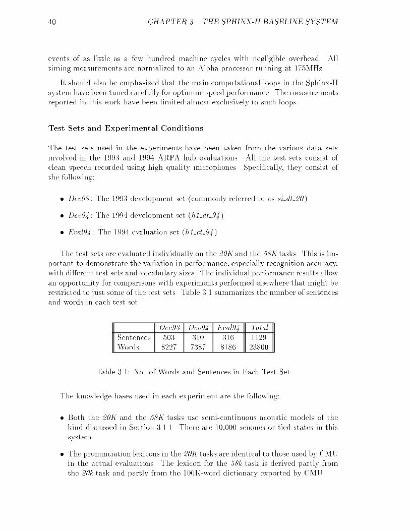
40 CHAPTER 3. THE SPHINX-II BASELINE SYSTEM
events of as little as a few hundred machine cycles with negligible overhead. Alltiming measurements are normalized to an Alpha processor running at 175MHz.
It should also be emphasized that the main computational loops in the Sphinx-IIsystem have been tuned carefully for optimum speed performance. The measurementsreported in this work have been limited almost exclusively to such loops.
Test Sets and Experimental Conditions
The test sets used in the experiments have been taken from the various data setsinvolved in the 1993 and 1994 ARPA hub evaluations. All the test sets consist ofclean speech recorded using high quality microphones. Speci�cally, they consist ofthe following:
� Dev93 : The 1993 development set (commonly referred to as si dt 20 ).
� Dev94 : The 1994 development set (h1 dt 94 ).
� Eval94 : The 1994 evaluation set (h1 et 94 ).
The test sets are evaluated individually on the 20K and the 58K tasks. This is im-portant to demonstrate the variation in performance, especially recognition accuracy,with di�erent test sets and vocabulary sizes. The individual performance results allowan opportunity for comparisons with experiments performed elsewhere that might berestricted to just some of the test sets. Table 3.1 summarizes the number of sentencesand words in each test set.
Dev93 Dev94 Eval94 Total
Sentences 503 310 316 1129Words 8227 7387 8186 23800
Table 3.1: No. of Words and Sentences in Each Test Set
The knowledge bases used in each experiment are the following:
� Both the 20K and the 58K tasks use semi-continuous acoustic models of thekind discussed in Section 3.1.1. There are 10,000 senones or tied states in thissystem.
� The pronunciation lexicons in the 20K tasks are identical to those used by CMUin the actual evaluations. The lexicon for the 58k task is derived partly fromthe 20k task and partly from the 100K-word dictionary exported by CMU.
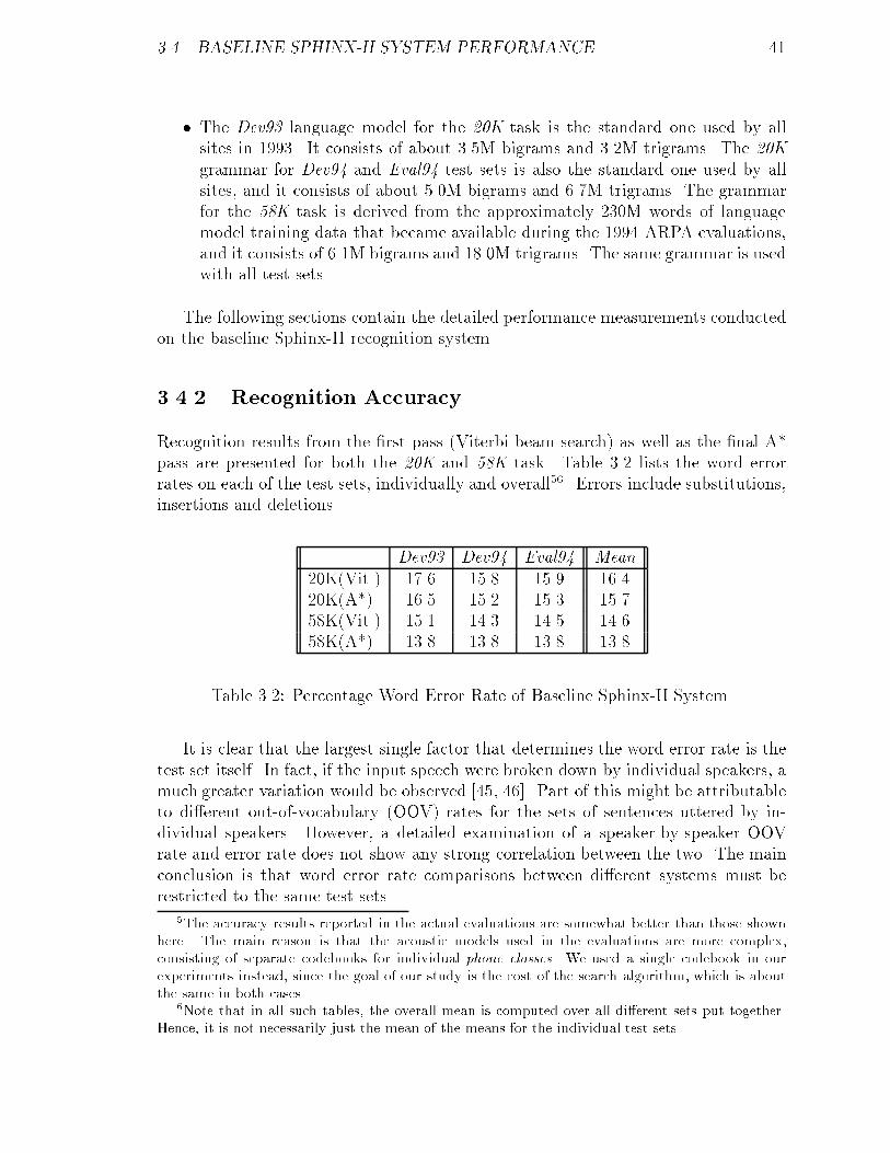
3.4. BASELINE SPHINX-II SYSTEM PERFORMANCE 41
� The Dev93 language model for the 20K task is the standard one used by allsites in 1993. It consists of about 3.5M bigrams and 3.2M trigrams. The 20Kgrammar for Dev94 and Eval94 test sets is also the standard one used by allsites, and it consists of about 5.0M bigrams and 6.7M trigrams. The grammarfor the 58K task is derived from the approximately 230M words of languagemodel training data that became available during the 1994 ARPA evaluations,and it consists of 6.1M bigrams and 18.0M trigrams. The same grammar is usedwith all test sets.
The following sections contain the detailed performance measurements conductedon the baseline Sphinx-II recognition system.
3.4.2 Recognition Accuracy
Recognition results from the �rst pass (Viterbi beam search) as well as the �nal A*pass are presented for both the 20K and 58K task. Table 3.2 lists the word errorrates on each of the test sets, individually and overall56. Errors include substitutions,insertions and deletions.
Dev93 Dev94 Eval94 Mean
20K(Vit.) 17.6 15.8 15.9 16.420K(A*) 16.5 15.2 15.3 15.758K(Vit.) 15.1 14.3 14.5 14.658K(A*) 13.8 13.8 13.8 13.8
Table 3.2: Percentage Word Error Rate of Baseline Sphinx-II System.
It is clear that the largest single factor that determines the word error rate is thetest set itself. In fact, if the input speech were broken down by individual speakers, amuch greater variation would be observed [45, 46]. Part of this might be attributableto di�erent out-of-vocabulary (OOV) rates for the sets of sentences uttered by in-dividual speakers. However, a detailed examination of a speaker-by-speaker OOVrate and error rate does not show any strong correlation between the two. The mainconclusion is that word error rate comparisons between di�erent systems must berestricted to the same test sets.
5The accuracy results reported in the actual evaluations are somewhat better than those shownhere. The main reason is that the acoustic models used in the evaluations are more complex,consisting of separate codebooks for individual phone classes. We used a single codebook in ourexperiments instead, since the goal of our study is the cost of the search algorithm, which is aboutthe same in both cases.
6Note that in all such tables, the overall mean is computed over all di�erent sets put together.Hence, it is not necessarily just the mean of the means for the individual test sets.
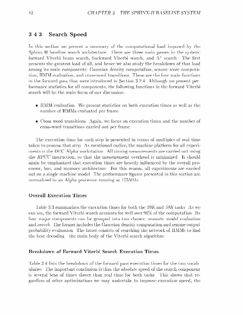
42 CHAPTER 3. THE SPHINX-II BASELINE SYSTEM
3.4.3 Search Speed
In this section we present a summary of the computational load imposed by theSphinx-II baseline search architecture. There are three main passes in the system:forward Viterbi beam search, backward Viterbi search, and A* search. The �rstpresents the greatest load of all, and hence we also study the breakdown of that loadamong its main components: Gaussian density computation, senone score computa-tion, HMM evaluation, and cross-word transitions. These are the four main functionsin the forward pass that were introduced in Section 3.2.4. Although we present per-formance statistics for all components, the following functions in the forward Viterbisearch will be the main focus of our discussion:
� HMM evaluation. We present statistics on both execution times as well as thenumber of HMMs evaluated per frame.
� Cross word transitions. Again, we focus on execution times and the number ofcross-word transitions carried out per frame.
The execution time for each step is presented in terms of multiples of real timetaken to process that step. As mentioned earlier, the machine platform for all experi-ments is the DEC Alpha workstation. All timing measurements are carried out usingthe RPCC instruction, so that the measurement overhead is minimized. It shouldagain be emphasized that execution times are heavily in uenced by the overall pro-cessor, bus, and memory architecture. For this reason, all experiments are carriedout on a single machine model. The performance �gures presented in this section arenormalized to an Alpha processor running at 175MHz.
Overall Execution Times
Table 3.3 summarizes the execution times for both the 20K and 58K tasks. As wecan see, the forward Viterbi search accounts for well over 90% of the computation. Itsfour major components can be grouped into two classes: acoustic model evaluationand search. The former includes the Gaussian density computation and senone outputprobability evaluation. The latter consists of searching the network of HMMs to �ndthe best decoding|the main body of the Viterbi search algorithm.
Breakdown of Forward Viterbi Search Execution Times
Table 3.4 lists the breakdown of the forward pass execution times for the two vocab-ularies. The important conclusion is that the absolute speed of the search componentis several tens of times slower than real time for both tasks. This shows that re-gardless of other optimizations we may undertake to improve execution speed, the
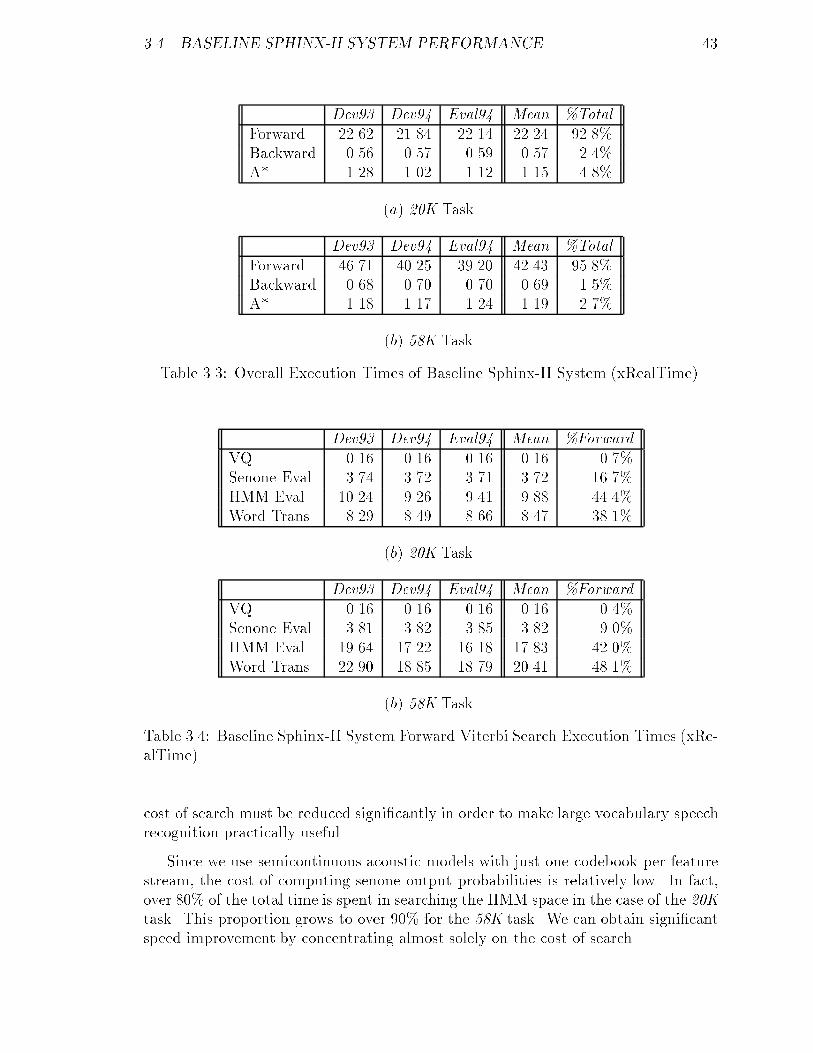
3.4. BASELINE SPHINX-II SYSTEM PERFORMANCE 43
Dev93 Dev94 Eval94 Mean %Total
Forward 22.62 21.84 22.14 22.24 92.8%Backward 0.56 0.57 0.59 0.57 2.4%A* 1.28 1.02 1.12 1.15 4.8%
(a) 20K Task.
Dev93 Dev94 Eval94 Mean %Total
Forward 46.71 40.25 39.20 42.43 95.8%Backward 0.68 0.70 0.70 0.69 1.5%A* 1.18 1.17 1.24 1.19 2.7%
(b) 58K Task.
Table 3.3: Overall Execution Times of Baseline Sphinx-II System (xRealTime).
Dev93 Dev94 Eval94 Mean %Forward
VQ 0.16 0.16 0.16 0.16 0.7%Senone Eval. 3.74 3.72 3.71 3.72 16.7%HMM Eval. 10.24 9.26 9.41 9.88 44.4%Word Trans. 8.29 8.49 8.66 8.47 38.1%
(b) 20K Task.
Dev93 Dev94 Eval94 Mean %Forward
VQ 0.16 0.16 0.16 0.16 0.4%Senone Eval. 3.81 3.82 3.85 3.82 9.0%HMM Eval. 19.64 17.22 16.18 17.83 42.0%Word Trans. 22.90 18.85 18.79 20.41 48.1%
(b) 58K Task.
Table 3.4: Baseline Sphinx-II System Forward Viterbi Search Execution Times (xRe-alTime).
cost of search must be reduced signi�cantly in order to make large vocabulary speechrecognition practically useful.
Since we use semicontinuous acoustic models with just one codebook per featurestream, the cost of computing senone output probabilities is relatively low. In fact,over 80% of the total time is spent in searching the HMM space in the case of the 20Ktask. This proportion grows to over 90% for the 58K task. We can obtain signi�cantspeed improvement by concentrating almost solely on the cost of search.
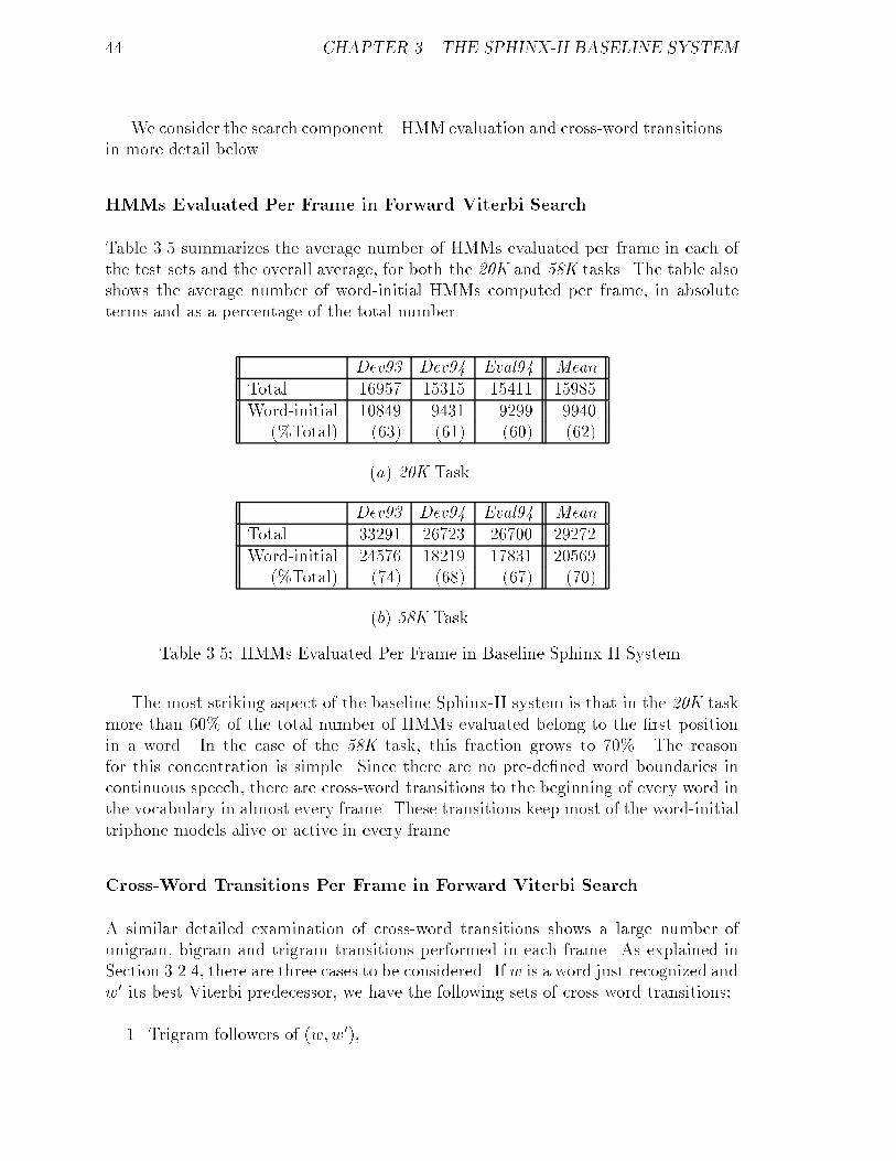
44 CHAPTER 3. THE SPHINX-II BASELINE SYSTEM
We consider the search component|HMMevaluation and cross-word transitions|in more detail below.
HMMs Evaluated Per Frame in Forward Viterbi Search
Table 3.5 summarizes the average number of HMMs evaluated per frame in each ofthe test sets and the overall average, for both the 20K and 58K tasks. The table alsoshows the average number of word-initial HMMs computed per frame, in absoluteterms and as a percentage of the total number.
Dev93 Dev94 Eval94 Mean
Total 16957 15315 15411 15985Word-initial 10849 9431 9299 9940
(%Total) (63) (61) (60) (62)
(a) 20K Task.
Dev93 Dev94 Eval94 Mean
Total 33291 26723 26700 29272Word-initial 24576 18219 17831 20569
(%Total) (74) (68) (67) (70)
(b) 58K Task.
Table 3.5: HMMs Evaluated Per Frame in Baseline Sphinx-II System.
The most striking aspect of the baseline Sphinx-II system is that in the 20K taskmore than 60% of the total number of HMMs evaluated belong to the �rst positionin a word. In the case of the 58K task, this fraction grows to 70%. The reasonfor this concentration is simple. Since there are no pre-de�ned word boundaries incontinuous speech, there are cross-word transitions to the beginning of every word inthe vocabulary in almost every frame. These transitions keep most of the word-initialtriphone models alive or active in every frame.
Cross-Word Transitions Per Frame in Forward Viterbi Search
A similar detailed examination of cross-word transitions shows a large number ofunigram, bigram and trigram transitions performed in each frame. As explained inSection 3.2.4, there are three cases to be considered. If w is a word just recognized andw0 its best Viterbi predecessor, we have the following sets of cross-word transitions:
1. Trigram followers of (w;w0),
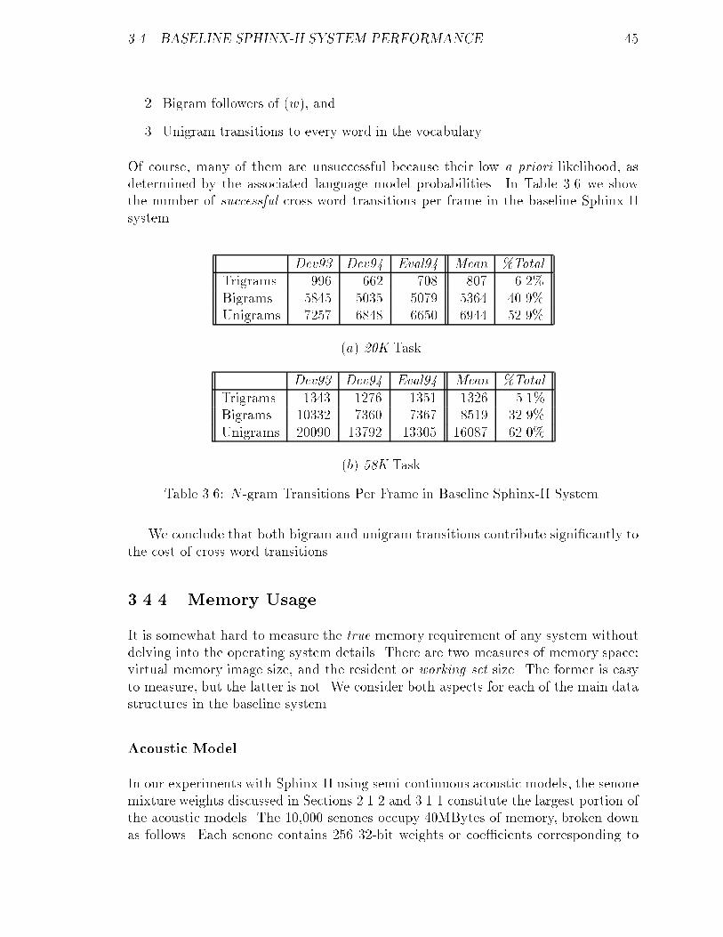
3.4. BASELINE SPHINX-II SYSTEM PERFORMANCE 45
2. Bigram followers of (w), and
3. Unigram transitions to every word in the vocabulary.
Of course, many of them are unsuccessful because their low a priori likelihood, asdetermined by the associated language model probabilities. In Table 3.6 we showthe number of successful cross-word transitions per frame in the baseline Sphinx-IIsystem.
Dev93 Dev94 Eval94 Mean %TotalTrigrams 996 662 708 807 6.2%Bigrams 5845 5035 5079 5364 40.9%Unigrams 7257 6848 6650 6944 52.9%
(a) 20K Task.
Dev93 Dev94 Eval94 Mean %Total
Trigrams 1343 1276 1351 1326 5.1%Bigrams 10332 7360 7367 8519 32.9%Unigrams 20090 13792 13305 16087 62.0%
(b) 58K Task.
Table 3.6: N -gram Transitions Per Frame in Baseline Sphinx-II System.
We conclude that both bigram and unigram transitions contribute signi�cantly tothe cost of cross-word transitions.
3.4.4 Memory Usage
It is somewhat hard to measure the true memory requirement of any system withoutdelving into the operating system details. There are two measures of memory space:virtual memory image size, and the resident or working set size. The former is easyto measure, but the latter is not. We consider both aspects for each of the main datastructures in the baseline system.
Acoustic Model
In our experiments with Sphinx-II using semi-continuous acoustic models, the senonemixture weights discussed in Sections 2.1.2 and 3.1.1 constitute the largest portion ofthe acoustic models. The 10,000 senones occupy 40MBytes of memory, broken downas follows. Each senone contains 256 32-bit weights or coe�cients corresponding to
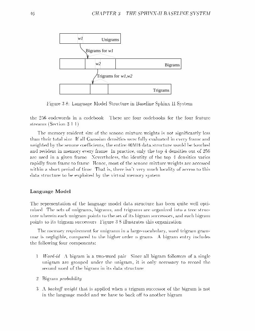
46 CHAPTER 3. THE SPHINX-II BASELINE SYSTEM
Unigrams
Bigrams
Trigrams
w1
w1
w1,w2
w2
Bigrams for
Trigrams for
Figure 3.8: Language Model Structure in Baseline Sphinx-II System.
the 256 codewords in a codebook. There are four codebooks for the four featurestreams (Section 3.1.1).
The memory resident size of the senone mixture weights is not signi�cantly lessthan their total size. If all Gaussian densities were fully evaluated in every frame andweighted by the senone coe�cients, the entire 40MB data structure would be touchedand resident in memory every frame. In practice, only the top 4 densities out of 256are used in a given frame. Nevertheless, the identity of the top 4 densities variesrapidly from frame to frame. Hence, most of the senone mixture weights are accessedwithin a short period of time. That is, there isn't very much locality of access to thisdata structure to be exploited by the virtual memory system.
Language Model
The representation of the language model data structure has been quite well opti-mized. The sets of unigrams, bigrams, and trigrams are organized into a tree struc-ture wherein each unigram points to the set of its bigram successors, and each bigrampoints to its trigram successors. Figure 3.8 illustrates this organization.
The memory requirement for unigrams in a large-vocabulary, word trigram gram-mar is negligible, compared to the higher-order n-grams. A bigram entry includesthe following four components:
1. Word-id. A bigram is a two-word pair. Since all bigram followers of a singleunigram are grouped under the unigram, it is only necessary to record thesecond word of the bigram in its data structure.
2. Bigram probability.
3. A backo� weight that is applied when a trigram successor of the bigram is notin the language model and we have to back o� to another bigram.

3.4. BASELINE SPHINX-II SYSTEM PERFORMANCE 47
4. Pointer to the trigram successors for the bigram.
Similarly, a trigram consists of 2 entries: a word-id and its trigram probability. Bymeans of a set of indirect lookup tables, each of the components of a bigram or trigramentry is compressed into 2 bytes. In other words, a single bigram requires 8 bytes,and a single trigram 4 bytes.
Based on these �gures, the two language models used in the 20K task (see Section3.4.1) occupy about 41MB and 67MB of memory, respectively. The 58K task languagemodel measures at about 121MB.
In this case, the di�culty faced by the virtual memory system in managing theworking set is that the granularity of access is usually much smaller than the physicalpage size of modern workstations. Many words have just a few 10s to 100s of bigramsuccessors. For example, the average number of bigrams per word in the case of the58K vocabulary is about 105. Whereas, the page size on a DEC Alpha is 8KB, 16KB,or more. Hence, much of the contents of a page of bigrams might be unused.
Search Data Structures
One of the search data structures is the network of active word HMMs in each frame.It is a dynamically varying quantity. The average number of active HMMs per frame,shown in Table 3.5, is a rough measure of this parameter. Its peak value, however, canbe substantially higher. Since all of the active HMMs in a frame have to be evaluated,they are all resident in memory. Other prominent search data structures include theforward and backward pass word lattices, the sizes of which grows approximatelyproportionately with the utterance length.
All of these data structures are relatively small compared to the acoustic andlanguage models, and we exclude them from further discussion.
Memory Usage Summary
In summary, the virtual memory requirement of the baseline system is well over100MB for the 20K tasks and around 200MB for the larger 58K task, excluding aux-iliary data structures used in the three passes. It is worth noting that the 20K tasksare on the verge of thrashing on a system with 128MB of main memory, indicatingthat most of the virtual pages are indeed being touched frequently.
48 CHAPTER 3. THE SPHINX-II BASELINE SYSTEM
3.5 Baseline System Summary
The purpose behind this chapter has been to outline the basic algorithms comprisingthe baseline Sphinx-II speech recognition system, as well as to evaluate its perfor-mance on large-vocabulary, continuous-speech tasks. We have obtained a measure ofits e�ciency along three basic dimensions: recognition accuracy, speed, and memoryrequirements. The evaluations were carried out on several test sets of read speechfrom the Wall Street Journal and North American Business News domains. The testsare run with two di�erent vocabulary sizes of 20K and 58K words.
The immediate conclusion from these measurements is that the baseline Sphinx-IIsystem cannot be used in practical, large vocabulary speech applications. Its compu-tational and memory requirements are an order of magnitude beyond the capabilitiesof commonly available workstations. While it is possible to improve the recognitionspeed by tightening the beam width (i.e., pruning the search more ruthlessly) and us-ing less sophisticated acoustic models to reduce memory requirements, such measurescannot overcome the inherent algorithmic complexities of the system. Moreover, theyalso result in an unacceptable increase in the recognition error rate.
We summarize our conclusions from this chapter:
� The main search of the full vocabulary, i.e. the forward Viterbi search, iscomputationally the most expensive. It accounts for over 90% of the total time.Postprocessing the word lattice is relatively inexpensive.
� The search component of the forward Viterbi search, even on modern high-endworkstations, is several tens of times slower than real time on large vocabulary,continuous speech tasks.
� About half of the search cost is attributable to HMM evaluation. Moreover, theactive HMMs to be evaluated during search are concentrated near the beginningof words. Speci�cally, over 60-70% of the active HMMs are word-initial models.This is not a new result. It has also been pointed out before, for example in[39, 43], although it has not been quanti�ed as systematically.
� The other half of the search cost is attributable to the evaluation of cross-word transitions, along with the need to perform several thousands of languagemodel accesses in each frame. Both bigram and unigram transitions contributesigni�cantly to this cost.
� The memory requirements of large vocabulary speech recognition systems aredominated by the two main databases: acoustic models and language models.For large tasks they can run between 100-200MB.
It is clear that in order for the state-of-the-art speech recognition systems to becomeuseful, we must address all of the above issues.

Chapter 4
Search Speed Optimization
4.1 Motivation
Most of the research e�ort on large vocabulary continuous speech recognition hasprimarily been in improving recognition accuracy, exempli�ed by the baseline Sphinx-II system. We have seen in the previous chapter that the Sphinx-II system is severaltens of times too slow and requires 100-200MB of memory for large vocabulary tasks.In order to be practically useful, speech recognition systems have to be e�cient intheir usage of computational resources as well.
There clearly are several real-time recognition systems around in the ARPA speechresearch community [23, 60, 55, 24]. However, the published literature is relativelybare regarding them. Their performance has never been formally evaluated with re-spect to the research systems or with respect to one another, in the way that theaccuracy of research systems has been. One goal of this thesis is to demonstratethat it is possible to achieve near real-time performance on large-vocabulary, contin-uous speech recognition tasks without compromising the recognition accuracy o�eredby research systems. This is a way of lending validity to the ongoing research onimproving accuracy.
We can also look at the current focus of speech research from the following angle.Speech recognition systems consist of two main components:
� Modelling structure, consisting of acoustic and language models.
� Algorithmic or search structure. For example, the forward pass Viterbi beamsearch algorithm described in the previous chapter.
Clearly, both components contribute to the various dimensions of e�ciency of thesystem|accuracy, speed, memory usage. But much of speech research has beenfocussed on the modelling aspect, speci�cally towards improving recognition accuracy.
49
50 CHAPTER 4. SEARCH SPEED OPTIMIZATION
This chapter concentrates on improving the algorithmic structure of search, whilepreserving the gains made in the modelling arena.
Another reason for concentrating on the search problem is the following. Thecomplexity of speech tasks is constantly growing, outpacing the growth in the powerof commonly available workstations. Since the late 1980s, the complexity of tasksundertaken by speech researchers has grown from the 1000-word Resource Manage-ment (RM) task [51] to essentially unlimited vocabulary tasks such as transcriptionof radio news broadcast in 1995 [48]. The RM task ran about an order of magnitudeslower than real time on processors of that day. The unlimited vocabulary tasks runabout two orders of magnitude slower than real time on modern workstations. Atleast part of the increase in the computational load is the increase in the search space.It seems reasonable to expect that task complexity will continue to grow in the future.
In this chapter, we discuss several algorithms and heuristics for improving thee�ciency of a recognition system. We use the Sphinx-II research system described inChapter 3 as a baseline for comparison. Since the focus of this work is in improvingsearch algorithms, we use the same acoustic and language models as in the baselinesystem. As mentioned above, there are two variables in speech recognition systems,modelling and search algorithms. By keeping one of them constant, we also ensurethat comparisons of the performance of proposed search algorithms with the baselinesystem are truly meaningful.
Though the work reported in this thesis has been carried out in the context of semi-continuous acoustic models, it is also relevant to systems that employ fully continuousmodels. At the time that this work was begun, the Sphinx-II semi-continuous acousticmodels were the best available to us. Over the last two years fully continuous acousticmodels [66, 5, 18] have become much more widely used in the speech community.They reduce the word error rate of recognition systems by a relative amount of about20-30% compared to semi-continuous acoustic models1 [46, 47]. The use of fullycontinuous models does not eliminate the search problem. On the other hand, the costof computing output probabilities for each state in each frame becomes much moresigni�cant that in the semi-continuous system. Hence, improving the speed of searchalone is not su�cient. We demonstrate that the proposed search algorithms usingsemi-continuous models generate compact word lattices with low lattice error rate.Such lattices can be postprocessed e�ciently using more complex acoustic models forhigher accuracy.
The outline of this chapter is as follows:
� In Section 4.2 we discuss lexical tree Viterbi search and all its design rami�ca-
1The contribution of acoustic modelling in di�erent systems to recognition accuracy is hard toestimate since some systems use not one but several sets of acoustic models, particularly for speakeradaptation [64]. The overall accuracy resulting from the use of continuous HMM models plus severalcycles of mean and variance adaptation was about 50% better than semi-continuous HMM modellingwith little or no adaptation.
4.2. LEXICAL TREE SEARCH 51
tions. We show how the lexical tree can be used to not only take advantage ofthe reduction in the number of active HMMs, but also to signi�cantly reducethe number of language model operations during cross-word transitions. Tree-structured lexicons are increasingly being used in all speech recognition systemsto take advantage of the sharing of HMMs across words, but this is the �rstinstance of reducing the language model operations signi�cantly. The sectionincludes detailed performance measurements and comparisons to the baselineSphinx-II system.
� In Section 4.3 we present an e�cient word lattice search to �nd a globallyoptimum path through the lattice using a trigram grammar. Even though thelexical tree search is about 20% worse in recognition accuracy relative to thebaseline system, most of the loss is recovered with this step. The global wordlattice search improves the recognition accuracy by considering alternative pathsthat are discarded during the lexical tree Viterbi search.
� In Section 4.4 we show that by rescoring the word lattice output of the treesearch using the conventional search algorithm of the baseline system, we es-sentially regain the recognition accuracy of the baseline system. Though ourrescoring experiments are restricted to semi-continuous acoustic models, clearlymore sophisticated models can be used as well.
� In Section 4.5 we propose a phonetic fast match heuristic that can be easilyintegrated into the lexical tree search algorithm to reduce the search, withvirtually no loss of accuracy. The heuristic uses senone output probabilities ineach frame to predict a set of active basephones near that frame. All others areconsidered inactive and pruned from search.
� There is a good deal of inherent parallelism at various levels in a speech recog-nition system. As commercial processor architectures and operating systemsbecome capable of supporting multithreaded applications, it becomes possibleto take advantage of the applications' inherent concurrency. In Section 4.6 weexplore the issues involved in exploiting them.
This chapter concludes with Section 4.7 that summarizes the performance of all ofthe techniques presented in this chapter.
4.2 Lexical Tree Search
The single largest source of computational e�ciency in performing search is in or-ganizing the HMMs to be searched as a phonetic tree, instead of the at structuredescribed in Section 3.2.1. It is referred to as a tree-structured lexicon or lexical tree

52 CHAPTER 4. SEARCH SPEED OPTIMIZATION
ABOUND AX B AW N DD
ABOUT AX B AW TD
ABOVE AX B AH V
BAKE B EY KD
BAKED B EY KD TD
BAKER B EY K AXR
BAKERY B EY K AXR IY
BAKING B EY K IX NG
(a) Example Pronunciation Lexicon.
AX B
AW
KD
VAH
TD
DDN
EY
AXR
IX
K
IY
NGB
TD
ABOUND
ABOUT
ABOVE
BAKE
BAKED
BAKER
BAKERY
BAKING
(b) Basephone Lexical Tree.
Figure 4.1: Basephone Lexical Tree Example.
structure. In such an organization, if the pronunciations of two or more words con-tain the same n initial phonemes, they share a single sequence of n HMM modelsrepresenting that initial portion of their pronunciation. Tree-structured lexicons haveoften been used in the past, especially in fast-match algorithms as a precursor step toa stack-decoding algorithm. More recently, tree search has come into widespread usein the main decoding process [43, 39]. Figure 4.1 shows a simple base-phone lexicaltree2 for a small example lexicon.
The lexical tree o�ers a potential solution to the two main sources of computationalcost in the baseline system:
� By introducing a high degree of sharing at the root nodes, it reduces the number
2Strictly speaking, the so-called lexical tree is actually a collection of trees or a forest, ratherthan a single tree. Nevertheless, we will continue to use the term lexical tree to signify the entirecollection.

4.2. LEXICAL TREE SEARCH 53
of word initial HMMs that need to be evaluated in each frame. As we saw inSection 3.4.3, word-initial HMMs are the most frequently evaluated HMMs inthe baseline system.
� The tree structure also greatly reduces the number of cross-word transitions,which is again a dominant part of search in the baseline system (see Section3.4.3, Table 3.6).
Another advantage of the tree organization is that both the number of active HMMsand the number of cross-word transitions grow much more slowly with increasingvocabulary size than in the case of a at lexical structure. On a per active HMMbasis, however, there is more work involved in the lexical tree search, since each activeHMM makes NULL transitions to several successor nodes, rather than just a singlenode as in the baseline system.
The main impediment to the full realization of the above advantages of tree searchis the incorporation of a language model into the search. In the at lexical structure,each cross-word transition from word wi to wj is accompanied by a language modelprobability P (wjjwi), assuming a bigram grammar. The di�culty with the tree struc-ture is that individual words are not identi�able at the roots of the tree. The rootnodes represent the beginning of several di�erent words (and hence multiple gram-mar states), which are related phonetically, but not grammatically. This can lead tocon icts between di�erent cross-word transitions that end up at the same root node.
Most of the current solutions rely on creating additional word HMM networks tohandle such con icts. The prominent ones have been reviewed in Section 2.4. Theobvious drawback associated with these solutions is an increase in the number ofoperations that the lexical tree structure is supposed to solve in the �rst place.
In this work we present a coherent solution that avoids the replication by post-poning the computation of language model probability for a word until the end of theword is reached. We show that this strategy improves the computational e�ciencyof search as it takes full advantage of the tree structure to dramatically reduce notonly the number of HMMs searched but also the number of cross-word transitionsand language model probabilities to be evaluated.
We �rst present the structure of the lexical tree in Section 4.2.1, followed by themain issue of treating language model probabilities across word transitions in Section4.2.2. The overall tree search algorithm is discussed in Section 4.2.3. Section 4.2.4contains a detailed performance analysis of this algorithm, and we �nally concludewith a summary in Section 4.2.5.
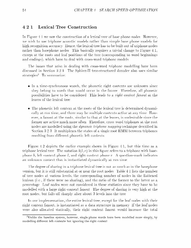
54 CHAPTER 4. SEARCH SPEED OPTIMIZATION
4.2.1 Lexical Tree Construction
In Figure 4.1 we saw the construction of a lexical tree of base phone nodes. However,we wish to use triphone acoustic models rather than simple base phone models forhigh recognition accuracy. Hence, the lexical tree has to be built out of triphone nodesrather than basephone nodes. This basically requires a trivial change to Figure 4.1,except at the roots and leaf positions of the tree (corresponding to word beginningsand endings), which have to deal with cross-word triphone models.
The issues that arise in dealing with cross-word triphone modelling have beendiscussed in Section 3.2.3. The Sphinx-II tree-structured decoder also uses similarstrategies3. To summarize:
� In a time-synchronous search, the phonetic right contexts are unknown sincethey belong to words that would occur in the future. Therefore, all phoneticpossibilities have to be considered. This leads to a right context fanout at theleaves of the lexical tree.
� The phonetic left context at the roots of the lexical tree is determined dynami-cally at run time, and there may be multiple contexts active at any time. How-ever, a fanout at the roots, similar to that at the leaves, is undesirable since theformer are active much more often. Therefore, cross-word triphones at the rootnodes are modelled using the dynamic triphone mapping technique described inSection 3.2.3. It multiplexes the states of a single root HMM between triphonesresulting from di�erent phonetic left contexts.
Figure 4.2 depicts the earlier example shown in Figure 4.1, but this time as atriphone lexical tree. The notation b(l; r) in this �gure refers to a triphone with base-phone b, left context phone l, and right context phone r. A question-mark indicatesan unknown context that is instantiated dynamically at run time.
The degree of sharing in a triphone lexical tree is not as much as in the basephoneversion, but it is still substantial at or near the root nodes. Table 4.1 lists the numberof tree nodes at various levels, the corresponding number of nodes in the attenedlexicon (i.e., if there were no sharing), and the ratio of the former to the latter as apercentage. Leaf nodes were not considered in these statistics since they have to bemodelled with a large right context fanout. The degree of sharing is very high at theroot nodes, but falls o� sharply after about 3 levels into the tree.
In our implementation, the entire lexical tree, except for the leaf nodes with theirright context fanout, is instantiated as a data structure in memory. If the leaf nodeswere also allocated statically, their right context fanout would increase the total
3Unlike the baseline system, however, single-phone words have been modelled more simply, bymodelling di�erent left contexts but ignoring the right context.
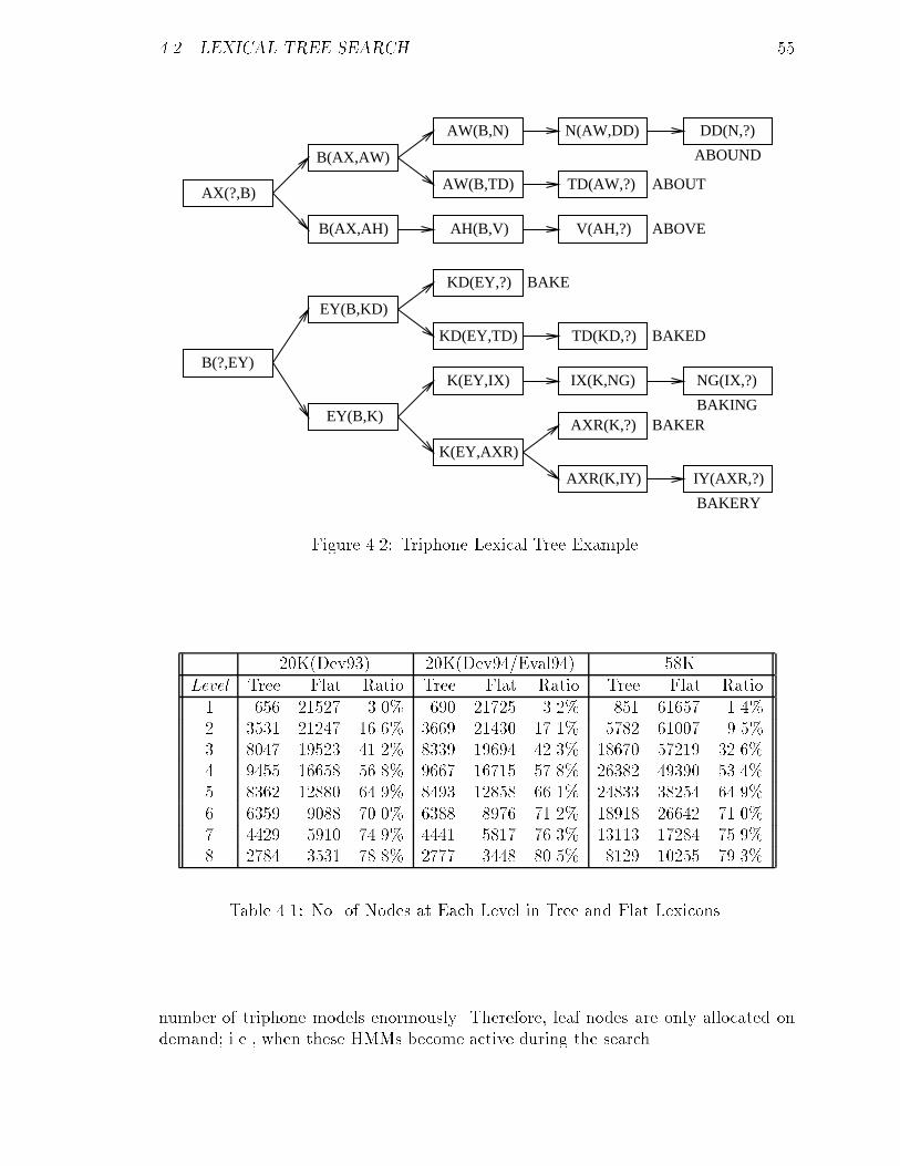
4.2. LEXICAL TREE SEARCH 55
KD(EY,TD)
V(AH,?)
TD(KD,?)
KD(EY,?)
K(EY,IX)
EY(B,K)
EY(B,KD)
B(?,EY)
DD(N,?)
TD(AW,?)
N(AW,DD)
AH(B,V)
AW(B,TD)
AW(B,N)
B(AX,AH)
B(AX,AW)
AX(?,B)
IY(AXR,?)
NG(IX,?)
AXR(K,IY)
AXR(K,?)
IX(K,NG)
K(EY,AXR)
ABOUND
ABOUT
ABOVE
BAKE
BAKED
BAKER
BAKERY
BAKING
Figure 4.2: Triphone Lexical Tree Example.
20K(Dev93) 20K(Dev94/Eval94) 58KLevel Tree Flat Ratio Tree Flat Ratio Tree Flat Ratio1 656 21527 3.0% 690 21725 3.2% 851 61657 1.4%2 3531 21247 16.6% 3669 21430 17.1% 5782 61007 9.5%3 8047 19523 41.2% 8339 19694 42.3% 18670 57219 32.6%4 9455 16658 56.8% 9667 16715 57.8% 26382 49390 53.4%5 8362 12880 64.9% 8493 12858 66.1% 24833 38254 64.9%6 6359 9088 70.0% 6388 8976 71.2% 18918 26642 71.0%7 4429 5910 74.9% 4441 5817 76.3% 13113 17284 75.9%8 2784 3531 78.8% 2777 3448 80.5% 8129 10255 79.3%
Table 4.1: No. of Nodes at Each Level in Tree and Flat Lexicons.
number of triphone models enormously. Therefore, leaf nodes are only allocated ondemand; i.e., when these HMMs become active during the search.

56 CHAPTER 4. SEARCH SPEED OPTIMIZATION
4.2.2 Incorporating Language Model Probabilities
The application of language model probabilities at word boundaries presents an inter-esting dilemma. Traditionally, the language model probability for a transition fromword wi to wj is computed and accumulated during the transition into the initial stateof wj. See, for example, the baseline system description in Section 3.2.4. As a result,the initial score for the new word wj is \primed" with the appropriate expectationfor that word in the context of the preceding history. This approach �ts neatly intothe Markov model and the Viterbi search algorithm, and has two main advantages:
� By using the language model probability upon word entry, the search processis biased in favour of the grammatically more likely words, and against the lesslikely ones. This bias serves to prune away the less likely words, reducing thedynamic search space.
� Frequently occurring short words or function words, such as a, the, an, of, etc.,which are generally poorly articulated, are given an initial boost by the languagemodel at the appropriate moments4. Thus, even though their poor articulationmight result in a poor acoustic match subsequently, the initial priming by thelanguage model often allows them to survive the beam search without gettingpruned.
The disadvantage of computing language model probabilities upon word entry is, ofcourse, the computational cost of evaluating a very large number of them in eachframe. This was seen in the previous chapter in Section 3.4.3, Table 3.4, making theexecution of cross-word transitions one of the most costly steps in the search process.
One would like to retain the advantages stated above, without incurring the asso-ciated cost, if possible. The immediate problem with a tree-structured lexicon is thatone does not have distinct, identi�able initial states for each word in the lexicon. Thetree structure implies that the root nodes are shared among several words, relatedphonetically, but quite unrelated grammatically. Hence it is not possible to determinea meaningful language model probability upon transitioning to a root node.
The Language Modelling Problem
Let us see the problem in detail by referring to Figure 4.3(a) and the original algorithmfor cross-word transitions in the baseline system in Figure 3.6. Figure 4.3(a) depictscross-words NULL transitions attempted from the �nal states of two words p1 and p2to the initial states of words w1 and w2 at time t. Let us represent the path scores
4The correct thing to do is, of course, to improve the acoustic modelling of such events ratherthan relying on the language model to overcome the former's shortcomings. However, every bithelps!
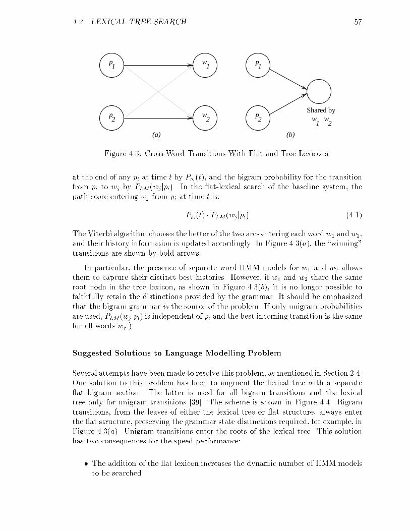
4.2. LEXICAL TREE SEARCH 57
w2
p1
p2
w1
w2
p1
p2 w
1
Shared by
(a) (b)
Figure 4.3: Cross-Word Transitions With Flat and Tree Lexicons.
at the end of any pi at time t by Ppi(t), and the bigram probability for the transitionfrom pi to wj by PLM (wjjpi). In the at-lexical search of the baseline system, thepath score entering wj from pi at time t is:
Ppi(t) � PLM (wjjpi) (4.1)
The Viterbi algorithm chooses the better of the two arcs entering each word w1 and w2,and their history information is updated accordingly. In Figure 4.3(a), the \winning"transitions are shown by bold arrows.
In particular, the presence of separate word-HMM models for w1 and w2 allowsthem to capture their distinct best histories. However, if w1 and w2 share the sameroot node in the tree lexicon, as shown in Figure 4.3(b), it is no longer possible tofaithfully retain the distinctions provided by the grammar. It should be emphasizedthat the bigram grammar is the source of the problem. If only unigram probabilitiesare used, PLM (wjjpi) is independent of pi and the best incoming transition is the samefor all words wj.)
Suggested Solutions to Language Modelling Problem
Several attempts have been made to resolve this problem, as mentioned in Section 2.4.One solution to this problem has been to augment the lexical tree with a separate at bigram section. The latter is used for all bigram transitions and the lexicaltree only for unigram transitions [39]. The scheme is shown in Figure 4.4. Bigramtransitions, from the leaves of either the lexical tree or at structure, always enterthe at structure, preserving the grammar state distinctions required, for example, inFigure 4.3(a). Unigram transitions enter the roots of the lexical tree. This solutionhas two consequences for the speed performance:
� The addition of the at lexicon increases the dynamic number of HMM modelsto be searched.
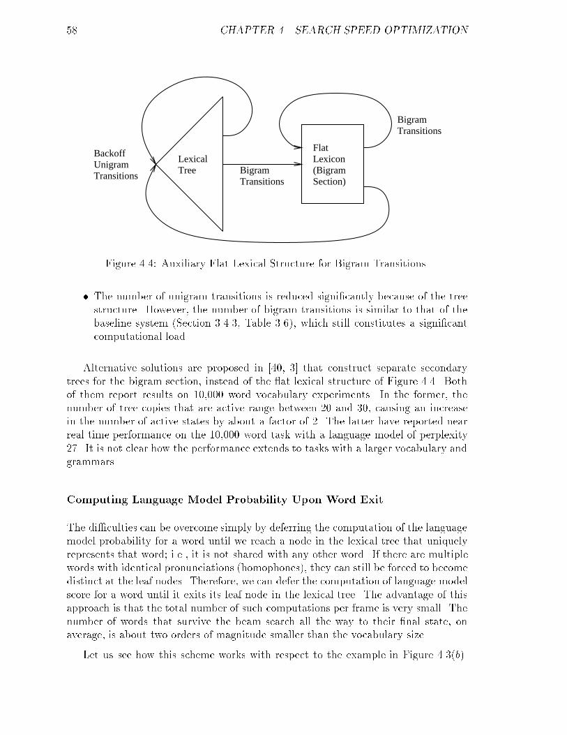
58 CHAPTER 4. SEARCH SPEED OPTIMIZATION
LexicalTree
FlatLexicon(BigramSection)
BigramTransitions
BigramTransitions
BackoffUnigramTransitions
Figure 4.4: Auxiliary Flat Lexical Structure for Bigram Transitions.
� The number of unigram transitions is reduced signi�cantly because of the treestructure. However, the number of bigram transitions is similar to that of thebaseline system (Section 3.4.3, Table 3.6), which still constitutes a signi�cantcomputational load.
Alternative solutions are proposed in [40, 3] that construct separate secondarytrees for the bigram section, instead of the at lexical structure of Figure 4.4. Bothof them report results on 10,000 word vocabulary experiments. In the former, thenumber of tree copies that are active range between 20 and 30, causing an increasein the number of active states by about a factor of 2. The latter have reported nearreal-time performance on the 10,000 word task with a language model of perplexity27. It is not clear how the performance extends to tasks with a larger vocabulary andgrammars.
Computing Language Model Probability Upon Word Exit
The di�culties can be overcome simply by deferring the computation of the languagemodel probability for a word until we reach a node in the lexical tree that uniquelyrepresents that word; i.e., it is not shared with any other word. If there are multiplewords with identical pronunciations (homophones), they can still be forced to becomedistinct at the leaf nodes. Therefore, we can defer the computation of language modelscore for a word until it exits its leaf node in the lexical tree. The advantage of thisapproach is that the total number of such computations per frame is very small. Thenumber of words that survive the beam search all the way to their �nal state, onaverage, is about two orders of magnitude smaller than the vocabulary size.
Let us see how this scheme works with respect to the example in Figure 4.3(b).
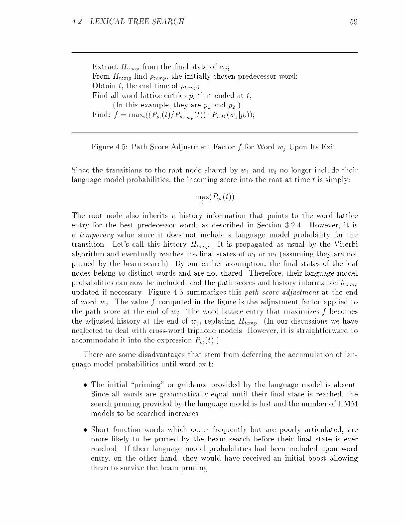
4.2. LEXICAL TREE SEARCH 59
Extract Htemp from the �nal state of wj;From Htemp �nd ptemp, the initially chosen predecessor word;Obtain t, the end time of ptemp;Find all word lattice entries pi that ended at t;
(In this example, they are p1 and p2.)Find: f = maxi((Ppi(t)=Pptemp(t)) � PLM (wjjpi));
Figure 4.5: Path Score Adjustment Factor f for Word wj Upon Its Exit.
Since the transitions to the root node shared by w1 and w2 no longer include theirlanguage model probabilities, the incoming score into the root at time t is simply:
maxi(Ppi(t))
The root node also inherits a history information that points to the word latticeentry for the best predecessor word, as described in Section 3.2.4. However, it isa temporary value since it does not include a language model probability for thetransition. Let's call this history Htemp. It is propagated as usual by the Viterbialgorithm and eventually reaches the �nal states of w1 or w2 (assuming they are notpruned by the beam search). By our earlier assumption, the �nal states of the leafnodes belong to distinct words and are not shared. Therefore, their language modelprobabilities can now be included, and the path scores and history information htemp
updated if necessary. Figure 4.5 summarizes this path score adjustment at the endof word wj. The value f computed in the �gure is the adjustment factor applied tothe path score at the end of wj . The word lattice entry that maximizes f becomesthe adjusted history at the end of wj, replacing Htemp. (In our discussions we haveneglected to deal with cross-word triphone models. However, it is straightforward toaccommodate it into the expression Ppi(t).)
There are some disadvantages that stem from deferring the accumulation of lan-guage model probabilities until word exit:
� The initial \priming" or guidance provided by the language model is absent.Since all words are grammatically equal until their �nal state is reached, thesearch pruning provided by the language model is lost and the number of HMMmodels to be searched increases.
� Short function words which occur frequently but are poorly articulated, aremore likely to be pruned by the beam search before their �nal state is everreached. If their language model probabilities had been included upon wordentry, on the other hand, they would have received an initial boost allowingthem to survive the beam pruning.

60 CHAPTER 4. SEARCH SPEED OPTIMIZATION
These concerns are addressed below.
Computing Language Model Probability When Entering Leaf Nodes
One obvious solution to the lack of guidance from a language model is to adopt anintermediate solution between computing the language model probability at the verybeginning upon word entry and at the very end upon word exit. Since the degreeof sharing in the lexical tree drops rapidly beyond 3 or 4 phone positions, one mightas well atten the lexical structure completely beyond that depth. For example, thelexical tree of Figure 4.2 is essentially at beginning at a depth of 4.
Since individual words are identi�able beyond a level of 3 or 4 from the roots,language model scores can be computed during the NULL transitions at these pointsin a similar fashion to that described above. Thus, the computational savings a�ordedby the tree structure are retained near the root where it matters most, and theguidance and search pruning provided by the language model is available when thetree structure ceases to be as e�ective.
However, the above solution still doesn't address the problem of poorly articulatedfunction words which are typically just 1-3 phones long. Secondly, the shorter we makethe depth of the actual tree structure and the earlier we compute language modelprobabilities, the more HMMs are actively being searched at that point, increasingthe cost of the path score adjustments.
For these reasons, in the �nal implementation of our tree search algorithm, thelanguage model probability for a word is computed upon entering the �nal leaf node5
for that word, rather than when exiting it. The algorithm is basically identical tothat shown in Figure 4.5, except that the path score adjustment is performed whenentering the �nal phone of wj, rather than exiting wj . Furthermore, it does not applyto single-phone words, which have to be treated essentially as in the baseline Sphinx-II system, outside the lexical tree structure. But this is not a major issue since thenumber of single-phone words in the vocabulary is only about 10.
For a short function word, this organization has the e�ect of accumulating thelanguage model probability early into the word, reducing the chances of its havingbeen pruned because of poor acoustic match. In particular, in the case of singlephone words, the language model probability is computed and accumulated uponword entry. This compromise partly retains the guidance provided by the languagemodel for poorly articulated short function words, while preserving computationale�ciency for the vast majority of the remaining words.
5Note that there are really several leaf nodes for any given word, caused by the right contextfanout for cross-word triphone modelling. However, we shall continue to speak loosely of a leaf node
in the singular, with the right context fanout being implicitly understood.
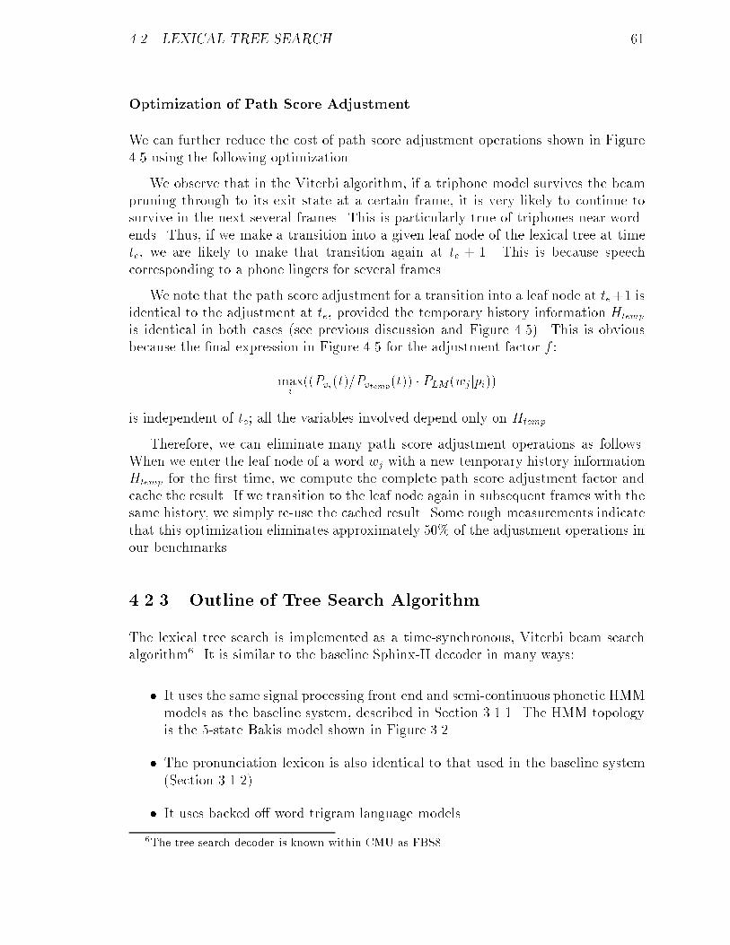
4.2. LEXICAL TREE SEARCH 61
Optimization of Path Score Adjustment
We can further reduce the cost of path score adjustment operations shown in Figure4.5 using the following optimization.
We observe that in the Viterbi algorithm, if a triphone model survives the beampruning through to its exit state at a certain frame, it is very likely to continue tosurvive in the next several frames. This is particularly true of triphones near word-ends. Thus, if we make a transition into a given leaf node of the lexical tree at timete, we are likely to make that transition again at te + 1. This is because speechcorresponding to a phone lingers for several frames.
We note that the path score adjustment for a transition into a leaf node at te+1 isidentical to the adjustment at te, provided the temporary history information Htemp
is identical in both cases (see previous discussion and Figure 4.5). This is obviousbecause the �nal expression in Figure 4.5 for the adjustment factor f :
maxi((Ppi(t)=Pptemp(t)) � PLM (wjjpi))
is independent of te; all the variables involved depend only on Htemp.
Therefore, we can eliminate many path score adjustment operations as follows.When we enter the leaf node of a word wj with a new temporary history informationHtemp for the �rst time, we compute the complete path score adjustment factor andcache the result. If we transition to the leaf node again in subsequent frames with thesame history, we simply re-use the cached result. Some rough measurements indicatethat this optimization eliminates approximately 50% of the adjustment operations inour benchmarks.
4.2.3 Outline of Tree Search Algorithm
The lexical tree search is implemented as a time-synchronous, Viterbi beam searchalgorithm6. It is similar to the baseline Sphinx-II decoder in many ways:
� It uses the same signal processing front end and semi-continuous phonetic HMMmodels as the baseline system, described in Section 3.1.1. The HMM topologyis the 5-state Bakis model shown in Figure 3.2.
� The pronunciation lexicon is also identical to that used in the baseline system(Section 3.1.2).
� It uses backed o� word trigram language models.
6The tree-search decoder is known within CMU as FBS8.
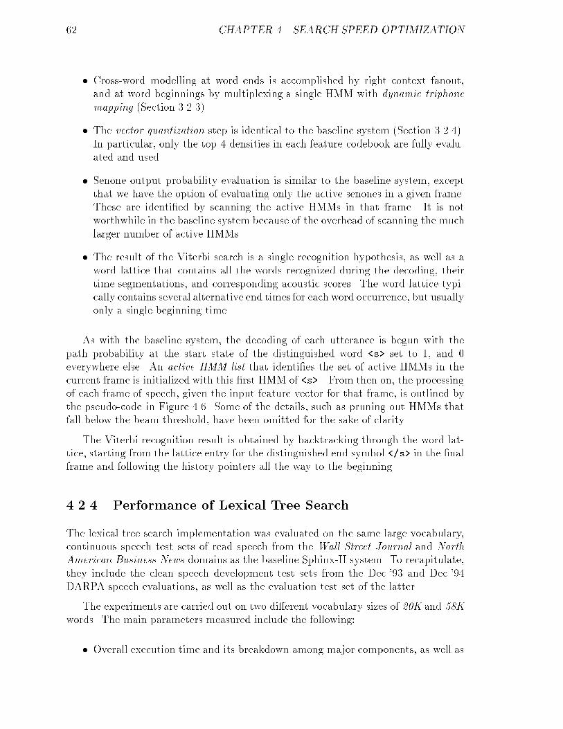
62 CHAPTER 4. SEARCH SPEED OPTIMIZATION
� Cross-word modelling at word ends is accomplished by right context fanout,and at word beginnings by multiplexing a single HMM with dynamic triphonemapping (Section 3.2.3).
� The vector quantization step is identical to the baseline system (Section 3.2.4).In particular, only the top 4 densities in each feature codebook are fully evalu-ated and used.
� Senone output probability evaluation is similar to the baseline system, exceptthat we have the option of evaluating only the active senones in a given frame.These are identi�ed by scanning the active HMMs in that frame. It is notworthwhile in the baseline system because of the overhead of scanning the muchlarger number of active HMMs.
� The result of the Viterbi search is a single recognition hypothesis, as well as aword lattice that contains all the words recognized during the decoding, theirtime segmentations, and corresponding acoustic scores. The word lattice typi-cally contains several alternative end times for each word occurrence, but usuallyonly a single beginning time.
As with the baseline system, the decoding of each utterance is begun with thepath probability at the start state of the distinguished word <s> set to 1, and 0everywhere else. An active HMM list that identi�es the set of active HMMs in thecurrent frame is initialized with this �rst HMM of <s> . From then on, the processingof each frame of speech, given the input feature vector for that frame, is outlined bythe pseudo-code in Figure 4.6. Some of the details, such as pruning out HMMs thatfall below the beam threshold, have been omitted for the sake of clarity.
The Viterbi recognition result is obtained by backtracking through the word lat-tice, starting from the lattice entry for the distinguished end symbol </s> in the �nalframe and following the history pointers all the way to the beginning.
4.2.4 Performance of Lexical Tree Search
The lexical tree search implementation was evaluated on the same large vocabulary,continuous speech test sets of read speech from the Wall Street Journal and NorthAmerican Business News domains as the baseline Sphinx-II system. To recapitulate,they include the clean speech development test sets from the Dec.'93 and Dec.'94DARPA speech evaluations, as well as the evaluation test set of the latter.
The experiments are carried out on two di�erent vocabulary sizes of 20K and 58Kwords. The main parameters measured include the following:
� Overall execution time and its breakdown among major components, as well as
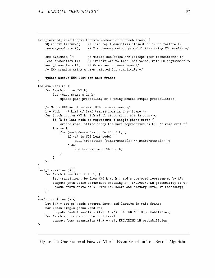
4.2. LEXICAL TREE SEARCH 63
tree_forward_frame (input feature vector for current frame) {
VQ (input feature); /* Find top 4 densities closest to input feature */
senone_evaluate (); /* Find senone output probabilities using VQ results */
hmm_evaluate (); /* Within-HMM/cross-HMM (except leaf transitions) */
leaf_transition (); /* Transitions to tree leaf nodes, with LM adjustment */
word_transition (); /* Cross-word transitions */
/* HMM pruning using a beam omitted for simplicity */
update active HMM list for next frame;
}
hmm_evaluate () {
for (each active HMM h)
for (each state s in h)
update path probability of s using senone output probabilities;
/* Cross-HMM and tree-exit NULL transitions */
L = NULL; /* List of leaf transitions in this frame */
for (each active HMM h with final state score within beam) {
if (h is leaf node or represents a single phone word) {
create word lattice entry for word represented by h; /* word exit */
} else {
for (each descendant node h' of h) {
if (h' is NOT leaf node)
NULL transition (final-state(h) -> start-state(h'));
else
add transition h->h' to L;
}
}
}
}
leaf_transition () {
for (each transition t in L) {
let transition t be from HMM h to h', and w the word represented by h';
compute path score adjustment entering h', INCLUDING LM probability of w;
update start state of h' with new score and history info, if necessary;
}
}
word_transition () {
let {w} = set of words entered into word lattice in this frame;
for (each single phone word w')
compute best transition ({w} -> w'), INCLUDING LM probabilities;
for (each root node r in lexical tree)
compute best transition ({w} -> r), EXCLUDING LM probabilities;
}
Figure 4.6: One Frame of Forward Viterbi Beam Search in Tree Search Algorithm.
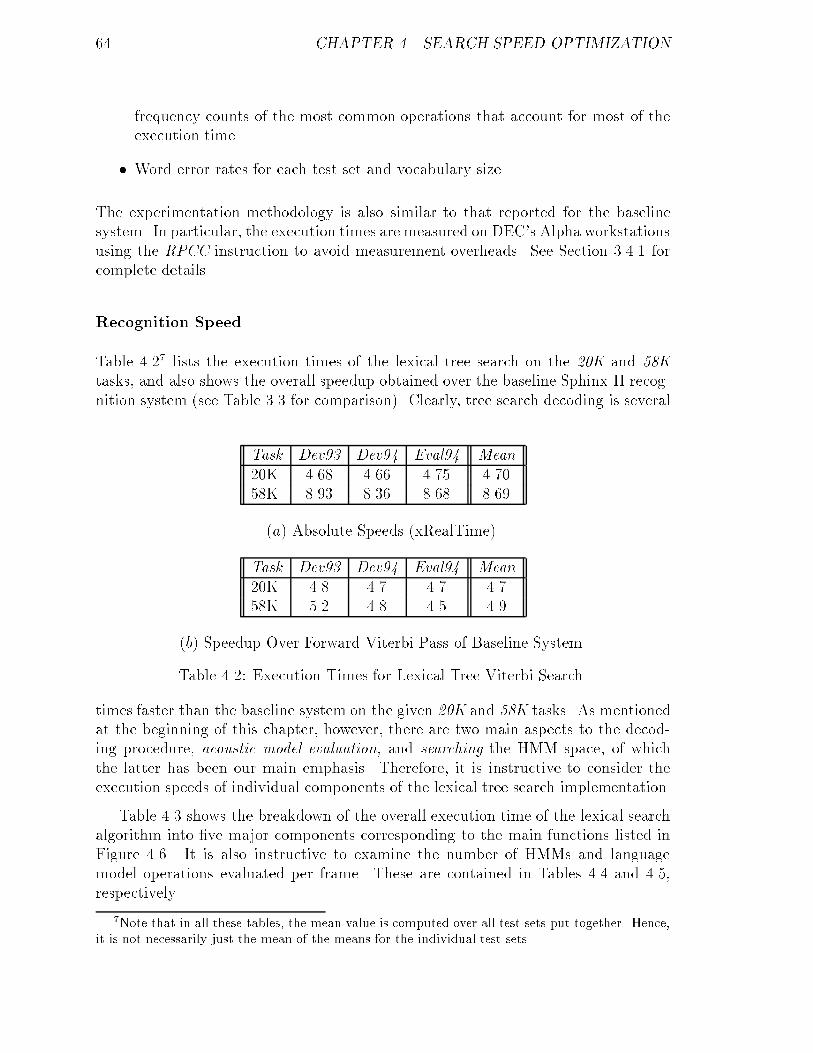
64 CHAPTER 4. SEARCH SPEED OPTIMIZATION
frequency counts of the most common operations that account for most of theexecution time.
� Word error rates for each test set and vocabulary size.
The experimentation methodology is also similar to that reported for the baselinesystem. In particular, the execution times are measured on DEC's Alpha workstationsusing the RPCC instruction to avoid measurement overheads. See Section 3.4.1 forcomplete details.
Recognition Speed
Table 4.27 lists the execution times of the lexical tree search on the 20K and 58Ktasks, and also shows the overall speedup obtained over the baseline Sphinx-II recog-nition system (see Table 3.3 for comparison). Clearly, tree search decoding is several
Task Dev93 Dev94 Eval94 Mean
20K 4.68 4.66 4.75 4.7058K 8.93 8.36 8.68 8.69
(a) Absolute Speeds (xRealTime).
Task Dev93 Dev94 Eval94 Mean
20K 4.8 4.7 4.7 4.758K 5.2 4.8 4.5 4.9
(b) Speedup Over Forward Viterbi Pass of Baseline System.
Table 4.2: Execution Times for Lexical Tree Viterbi Search.
times faster than the baseline system on the given 20K and 58K tasks. As mentionedat the beginning of this chapter, however, there are two main aspects to the decod-ing procedure, acoustic model evaluation, and searching the HMM space, of whichthe latter has been our main emphasis. Therefore, it is instructive to consider theexecution speeds of individual components of the lexical tree search implementation.
Table 4.3 shows the breakdown of the overall execution time of the lexical searchalgorithm into �ve major components corresponding to the main functions listed inFigure 4.6. It is also instructive to examine the number of HMMs and languagemodel operations evaluated per frame. These are contained in Tables 4.4 and 4.5,respectively.
7Note that in all these tables, the mean value is computed over all test sets put together. Hence,it is not necessarily just the mean of the means for the individual test sets.
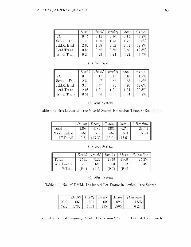
4.2. LEXICAL TREE SEARCH 65
Dev93 Dev94 Eval94 Mean %Total
VQ 0.15 0.15 0.16 0.15 3.2%Senone Eval. 1.73 1.70 1.73 1.72 36.6%HMM Eval. 2.02 1.98 2.02 2.01 42.8%Leaf Trans. 0.56 0.58 0.60 0.58 12.3%Word Trans. 0.20 0.23 0.24 0.22 4.7%
(a) 20K System.
Dev93 Dev94 Eval94 Mean %Total
VQ 0.16 0.17 0.17 0.16 1.8%Senone Eval. 2.39 2.27 2.32 2.33 26.8%HMM Eval. 3.78 3.57 3.71 3.70 42.6%Leaf Trans. 2.08 1.81 1.91 1.94 22.3%Word Trans. 0.51 0.56 0.57 0.54 6.2%
(b) 58K System.
Table 4.3: Breakdown of Tree Viterbi Search Execution Times (xRealTime).
Dev93 Dev94 Eval94 Mean %Baseline
Total 4298 4181 4281 4259 26.6%Word-initial 551 556 557 554 5.6%
(%Total) (12.8) (13.3) (13.0) (13.0)
(a) 20K System.
Dev93 Dev94 Eval94 Mean %Baseline
Total 7561 7122 7358 7369 25.2%Word-initial 711 680 683 693 3.4%
%Total (9.4) (9.5) (9.3) (9.4)
(b) 58K System.
Table 4.4: No. of HMMs Evaluated Per Frame in Lexical Tree Search.
Dev93 Dev94 Eval94 Mean %Baseline
20K 663 591 609 625 4.8%58K 1702 1493 1558 1595 6.2%
Table 4.5: No. of Language Model Operations/Frame in Lexical Tree Search.
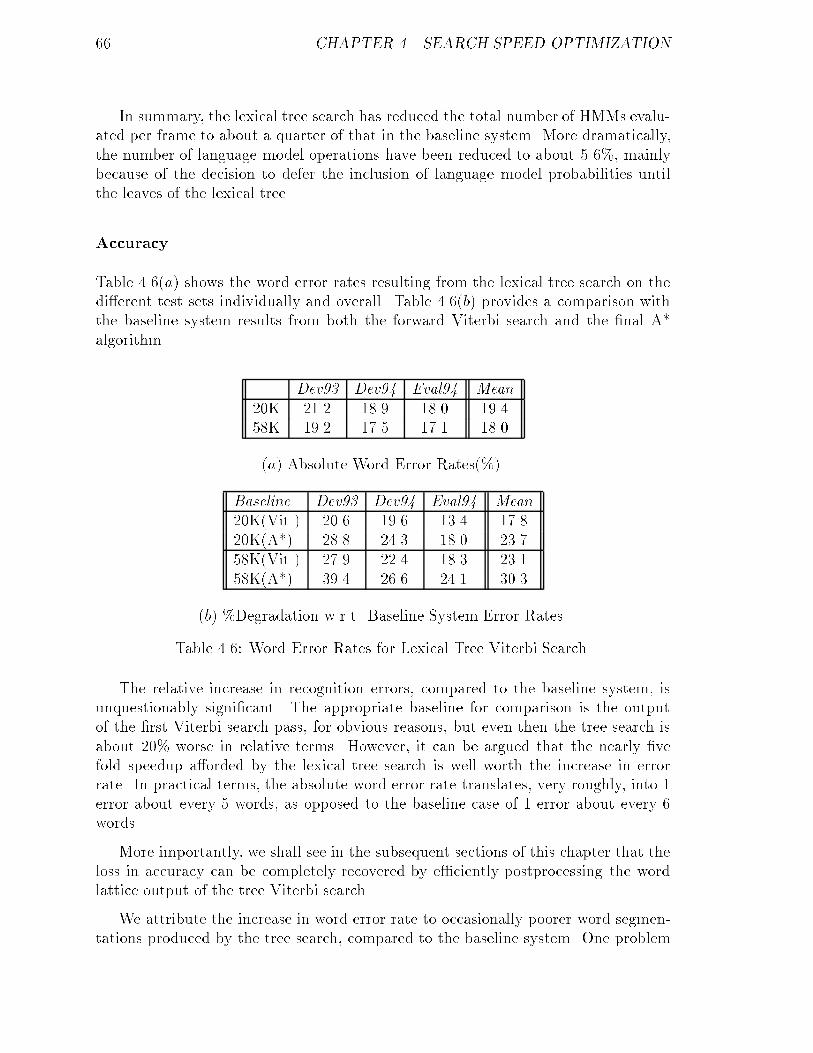
66 CHAPTER 4. SEARCH SPEED OPTIMIZATION
In summary, the lexical tree search has reduced the total number of HMMs evalu-ated per frame to about a quarter of that in the baseline system. More dramatically,the number of language model operations have been reduced to about 5-6%, mainlybecause of the decision to defer the inclusion of language model probabilities untilthe leaves of the lexical tree.
Accuracy
Table 4.6(a) shows the word error rates resulting from the lexical tree search on thedi�erent test sets individually and overall. Table 4.6(b) provides a comparison withthe baseline system results from both the forward Viterbi search and the �nal A*algorithm.
Dev93 Dev94 Eval94 Mean
20K 21.2 18.9 18.0 19.458K 19.2 17.5 17.1 18.0
(a) Absolute Word Error Rates(%).
Baseline Dev93 Dev94 Eval94 Mean20K(Vit.) 20.6 19.6 13.4 17.820K(A*) 28.8 24.3 18.0 23.758K(Vit.) 27.9 22.4 18.3 23.158K(A*) 39.4 26.6 24.1 30.3
(b) %Degradation w.r.t. Baseline System Error Rates.
Table 4.6: Word Error Rates for Lexical Tree Viterbi Search.
The relative increase in recognition errors, compared to the baseline system, isunquestionably signi�cant. The appropriate baseline for comparison is the outputof the �rst Viterbi search pass, for obvious reasons, but even then the tree search isabout 20% worse in relative terms. However, it can be argued that the nearly �vefold speedup a�orded by the lexical tree search is well worth the increase in errorrate. In practical terms, the absolute word error rate translates, very roughly, into 1error about every 5 words, as opposed to the baseline case of 1 error about every 6words.
More importantly, we shall see in the subsequent sections of this chapter that theloss in accuracy can be completely recovered by e�ciently postprocessing the wordlattice output of the tree Viterbi search.
We attribute the increase in word error rate to occasionally poorer word segmen-tations produced by the tree search, compared to the baseline system. One problem
4.2. LEXICAL TREE SEARCH 67
is that Viterbi search is a greedy algorithm that follows a local maximum. In eachframe, the root nodes of the lexical tree receive several incoming, cross-word transi-tions (from the �nal states of the leaves of the tree), of which the best is chosen bythe Viterbi algorithm. The same is true in the case of the baseline system with a at lexical structure. However, in the latter, each cross-word transition is augmentedwith a grammar probability so that the e�ective fan-in is reduced. This is not possiblewith the tree structure, with the result that the Viterbi pruning behaviour at treeroots is modi�ed.
4.2.5 Lexical Tree Search Summary
Clearly, the results from the lexical tree search algorithm are mixed. On the one hand,there is a nearly 5-fold overall increase in recognition speed, but it is accompanied byan approximately 20% increase in word error rate, relative to the baseline system. Weshall see in subsequent sections that we can, not surprisingly, recover from the lossin accuracy by postprocessing the word lattice output of the tree search algorithm.Some of the other conclusions to be drawn in this section are the following:
� While the overall speedup is slightly under 5, the search speed alone, excludingsenone output probability computation, is over 6 times faster than the baselinecase (comparing Tables 4.3 and 3.4). This is an important result since our focusin this section has been improving the speed of searching the HMM space.
� It should be pointed out that the reduction in search speed is irrelevant ifthe cost of computing state output probabilities is overwhelming. Thus, it isappropriate to rely on a detailed tree search if we are using semi-continuous oreven discrete acoustic models, but it is less relevant for fully continuous ones.
� Using semi-continuous acoustic models, we obtain a word lattice that is ex-tremely compact. The total number of words in the lattice is, on average, sev-eral hundreds to a few thousand for an average sentence of 10sec duration (1000frames). Furthermore, the lattice error rate|the fraction of correct words notfound in the lattice around the expected time|is extremely small. It is about2%, excluding out-of-vocabulary words. This is substantially the same as thelattice error rate of the baseline Sphinx-II system, and similar to the resultsreported in [65]. The compact nature of the word lattice, combined with itslow error rate, makes it an ideal input for further postprocessing using moredetailed acoustic models and search algorithms.
The lexical tree described in this section can be contrasted to those described in[40, 3, 39, 43] in their treatment of the language model. By deferring the application oflanguage model probabilities to the leaves of the tree, we gain a signi�cant reductionin computation.
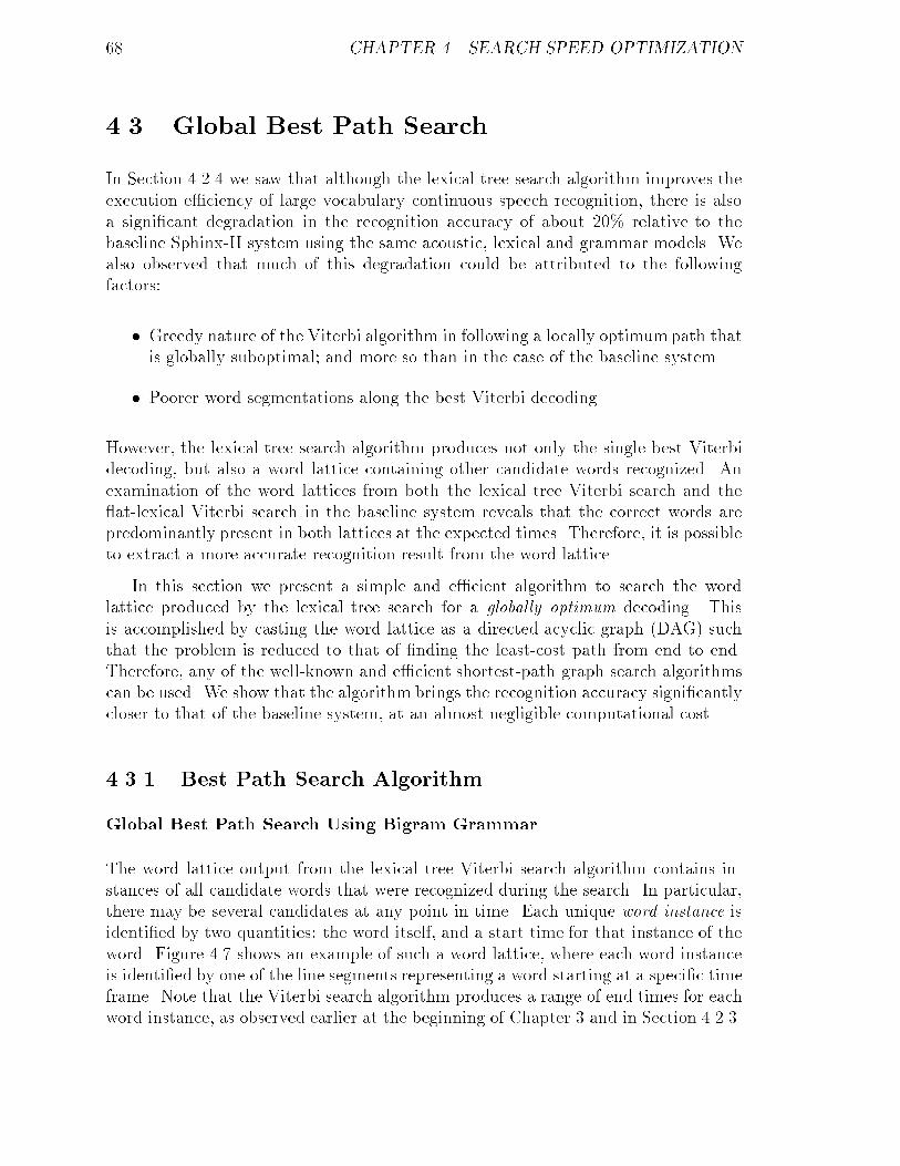
68 CHAPTER 4. SEARCH SPEED OPTIMIZATION
4.3 Global Best Path Search
In Section 4.2.4 we saw that although the lexical tree search algorithm improves theexecution e�ciency of large vocabulary continuous speech recognition, there is alsoa signi�cant degradation in the recognition accuracy of about 20% relative to thebaseline Sphinx-II system using the same acoustic, lexical and grammar models. Wealso observed that much of this degradation could be attributed to the followingfactors:
� Greedy nature of the Viterbi algorithm in following a locally optimumpath thatis globally suboptimal; and more so than in the case of the baseline system.
� Poorer word segmentations along the best Viterbi decoding.
However, the lexical tree search algorithm produces not only the single best Viterbidecoding, but also a word lattice containing other candidate words recognized. Anexamination of the word lattices from both the lexical tree Viterbi search and the at-lexical Viterbi search in the baseline system reveals that the correct words arepredominantly present in both lattices at the expected times. Therefore, it is possibleto extract a more accurate recognition result from the word lattice.
In this section we present a simple and e�cient algorithm to search the wordlattice produced by the lexical tree search for a globally optimum decoding. Thisis accomplished by casting the word lattice as a directed acyclic graph (DAG) suchthat the problem is reduced to that of �nding the least-cost path from end to end.Therefore, any of the well-known and e�cient shortest-path graph search algorithmscan be used. We show that the algorithm brings the recognition accuracy signi�cantlycloser to that of the baseline system, at an almost negligible computational cost.
4.3.1 Best Path Search Algorithm
Global Best Path Search Using Bigram Grammar
The word lattice output from the lexical tree Viterbi search algorithm contains in-stances of all candidate words that were recognized during the search. In particular,there may be several candidates at any point in time. Each unique word instance isidenti�ed by two quantities: the word itself, and a start time for that instance of theword. Figure 4.7 shows an example of such a word lattice, where each word instanceis identi�ed by one of the line segments representing a word starting at a speci�c timeframe. Note that the Viterbi search algorithm produces a range of end times for eachword instance, as observed earlier at the beginning of Chapter 3 and in Section 4.2.3.
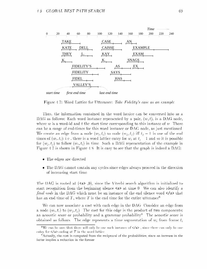
4.3. GLOBAL BEST PATH SEARCH 69
0 20 40 60 80 100 120 140 160 180 200 220 240
THEY
K.
KATE
TAKE
FIDEL
FIDELITY
FIDELITY’S
VALLEY’S
CASE
AS
SAYS
K.
KAY EXAM
EXAMPLE
AN
CAISSE
SNAGS
DELL
L.
HAS
EX
start time first end time last end time
Time
Figure 4.7: Word Lattice for Utterance: Take Fidelity's case as an example.
Thus, the information contained in the word lattice can be converted into as aDAG as follows: Each word instance represented by a pair, (w; t), is a DAG node,where w is a word-id and t the start time corresponding to this instance of w. Therecan be a range of end-times for this word instance or DAG node, as just mentioned.We create an edge from a node (wi; ti) to node (wj; tj) i� tj � 1 is one of the endtimes of (wi; ti); i.e., there is a word lattice entry for wi at tj � 1 and so it is possiblefor (wj; tj) to follow (wi; ti) in time. Such a DAG representation of the example inFigure 4.7 is shown in Figure 4.8. It is easy to see that the graph is indeed a DAG:
� The edges are directed.
� The DAG cannot contain any cycles since edges always proceed in the directionof increasing start time.
The DAG is rooted at (<s> ,0), since the Viterbi search algorithm is initialized tostart recognition from the beginning silence <s> at time 0. We can also identify a�nal node in the DAG which must be an instance of the end silence word </s> thathas an end time of T , where T is the end time for the entire utterance8.
We can now associate a cost with each edge in the DAG. Consider an edge froma node (wi; ti) to (wj; tj). The cost for this edge is the product of two components:an acoustic score or probability and a grammar probability9. The acoustic score isobtained as follows. The edge represents a time segmentation of wi from frame ti
8We can be sure that there will only be one such instance of </s> , since there can only be oneentry for </s> ending at T in the word lattice.
9Actually, the cost is computed from the reciprocal of the probabilities, since an increase in thelatter implies a reduction in the former.
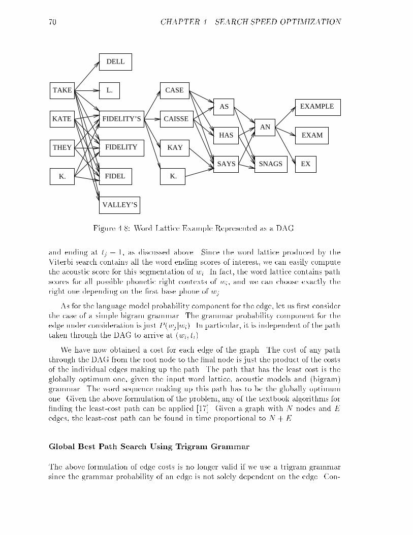
70 CHAPTER 4. SEARCH SPEED OPTIMIZATION
TAKE
KATE
THEY
K.
FIDELITY’S
FIDELITY
FIDEL
VALLEY’S
DELL
L. CASE
CAISSE
KAY
K.
AS
SAYS
HASAN
SNAGS
EXAMPLE
EXAM
EX
Figure 4.8: Word Lattice Example Represented as a DAG.
and ending at tj � 1, as discussed above. Since the word lattice produced by theViterbi search contains all the word-ending scores of interest, we can easily computethe acoustic score for this segmentation of wi. In fact, the word lattice contains pathscores for all possible phonetic right contexts of wi, and we can choose exactly theright one depending on the �rst base phone of wj.
As for the language model probability component for the edge, let us �rst considerthe case of a simple bigram grammar. The grammar probability component for theedge under consideration is just P (wj jwi). In particular, it is independent of the pathtaken through the DAG to arrive at (wi; ti).
We have now obtained a cost for each edge of the graph. The cost of any paththrough the DAG from the root node to the �nal node is just the product of the costsof the individual edges making up the path. The path that has the least cost is theglobally optimum one, given the input word lattice, acoustic models and (bigram)grammar. The word sequence making up this path has to be the globally optimumone. Given the above formulation of the problem, any of the textbook algorithms for�nding the least-cost path can be applied [17]. Given a graph with N nodes and Eedges, the least-cost path can be found in time proportional to N + E.
Global Best Path Search Using Trigram Grammar
The above formulation of edge costs is no longer valid if we use a trigram grammarsince the grammar probability of an edge is not solely dependent on the edge. Con-
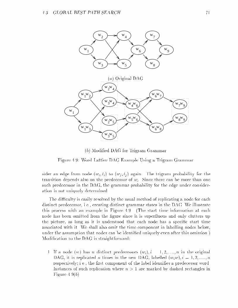
4.3. GLOBAL BEST PATH SEARCH 71
w1
w2
w3
w4
w5
w6
w7
w8
w9
(a) Original DAG.
w1w
2
w1w
3
w2w
4
w3w
4
w2w
5
w3w
5
w4w
6
w5w
6
w6w
7
w6w
8
w7w
9
w8w
9
w1
(b) Modi�ed DAG for Trigram Grammar.
Figure 4.9: Word Lattice DAG Example Using a Trigram Grammar.
sider an edge from node (wi; ti) to (wj; tj) again. The trigram probability for thetransition depends also on the predecessor of wi. Since there can be more than onesuch predecessor in the DAG, the grammar probability for the edge under consider-ation is not uniquely determined.
The di�culty is easily resolved by the usual method of replicating a node for eachdistinct predecessor, i.e., creating distinct grammar states in the DAG. We illustratethis process with an example in Figure 4.9. (The start time information at eachnode has been omitted from the �gure since it is super uous and only clutters upthe picture, as long as it is understood that each node has a speci�c start timeassociated with it. We shall also omit the time component in labelling nodes below,under the assumption that nodes can be identi�ed uniquely even after this omission.)Modi�cation to the DAG is straightforward:
1. If a node (w) has n distinct predecessors (wi); i = 1; 2; : : : ; n in the originalDAG, it is replicated n times in the new DAG, labelled (wiw); i = 1; 2; : : : ; nrespectively; i.e., the �rst component of the label identi�es a predecessor word.Instances of such replication where n > 1 are marked by dashed rectangles inFigure 4.9(b).
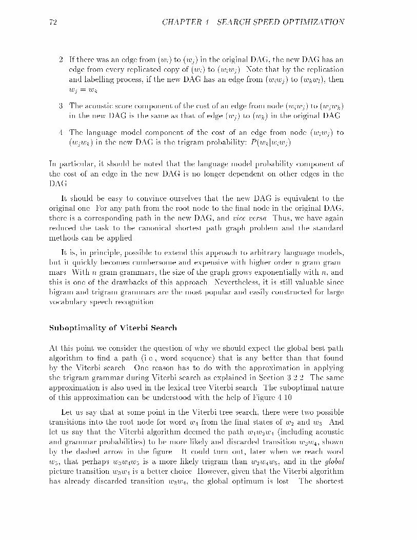
72 CHAPTER 4. SEARCH SPEED OPTIMIZATION
2. If there was an edge from (wi) to (wj) in the original DAG, the new DAG has anedge from every replicated copy of (wi) to (wiwj). Note that by the replicationand labelling process, if the new DAG has an edge from (wiwj) to (wkwl), thenwj = wk.
3. The acoustic score component of the cost of an edge from node (wiwj) to (wjwk)in the new DAG is the same as that of edge (wj) to (wk) in the original DAG.
4. The language model component of the cost of an edge from node (wiwj) to(wjwk) in the new DAG is the trigram probability: P (wkjwiwj).
In particular, it should be noted that the language model probability component ofthe cost of an edge in the new DAG is no longer dependent on other edges in theDAG.
It should be easy to convince ourselves that the new DAG is equivalent to theoriginal one. For any path from the root node to the �nal node in the original DAG,there is a corresponding path in the new DAG, and vice versa. Thus, we have againreduced the task to the canonical shortest path graph problem and the standardmethods can be applied.
It is, in principle, possible to extend this approach to arbitrary language models,but it quickly becomes cumbersome and expensive with higher order n-gram gram-mars. With n-gram grammars, the size of the graph grows exponentially with n, andthis is one of the drawbacks of this approach. Nevertheless, it is still valuable sincebigram and trigram grammars are the most popular and easily constructed for largevocabulary speech recognition.
Suboptimality of Viterbi Search
At this point we consider the question of why we should expect the global best pathalgorithm to �nd a path (i.e., word sequence) that is any better than that foundby the Viterbi search. One reason has to do with the approximation in applyingthe trigram grammar during Viterbi search as explained in Section 3.2.2. The sameapproximation is also used in the lexical tree Viterbi search. The suboptimal natureof this approximation can be understood with the help of Figure 4.10.
Let us say that at some point in the Viterbi tree search, there were two possibletransitions into the root node for word w4 from the �nal states of w2 and w3. Andlet us say that the Viterbi algorithm deemed the path w1w2w4 (including acousticand grammar probabilities) to be more likely and discarded transition w3w4, shownby the dashed arrow in the �gure. It could turn out, later when we reach wordw5, that perhaps w3w4w5 is a more likely trigram than w2w4w5, and in the globalpicture transition w3w4 is a better choice. However, given that the Viterbi algorithmhas already discarded transition w3w4, the global optimum is lost. The shortest
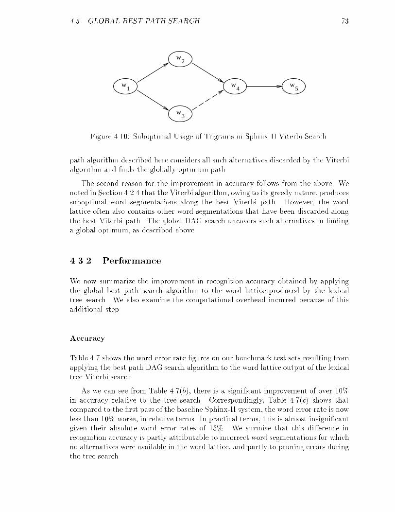
4.3. GLOBAL BEST PATH SEARCH 73
w1
w2
w3
w4
w5
Figure 4.10: Suboptimal Usage of Trigrams in Sphinx-II Viterbi Search.
path algorithm described here considers all such alternatives discarded by the Viterbialgorithm and �nds the globally optimum path.
The second reason for the improvement in accuracy follows from the above. Wenoted in Section 4.2.4 that the Viterbi algorithm, owing to its greedy nature, producessuboptimal word segmentations along the best Viterbi path. However, the wordlattice often also contains other word segmentations that have been discarded alongthe best Viterbi path. The global DAG search uncovers such alternatives in �ndinga global optimum, as described above.
4.3.2 Performance
We now summarize the improvement in recognition accuracy obtained by applyingthe global best path search algorithm to the word lattice produced by the lexicaltree search. We also examine the computational overhead incurred because of thisadditional step.
Accuracy
Table 4.7 shows the word error rate �gures on our benchmark test sets resulting fromapplying the best path DAG search algorithm to the word lattice output of the lexicaltree Viterbi search.
As we can see from Table 4.7(b), there is a signi�cant improvement of over 10%in accuracy relative to the tree search. Correspondingly, Table 4.7(c) shows thatcompared to the �rst pass of the baseline Sphinx-II system, the word error rate is nowless than 10% worse, in relative terms. In practical terms, this is almost insigni�cantgiven their absolute word error rates of 15%. We surmise that this di�erence inrecognition accuracy is partly attributable to incorrect word segmentations for whichno alternatives were available in the word lattice, and partly to pruning errors duringthe tree search.
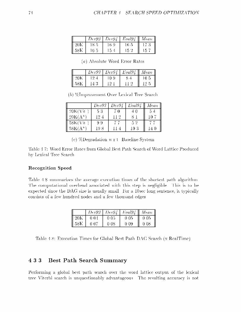
74 CHAPTER 4. SEARCH SPEED OPTIMIZATION
Dev93 Dev94 Eval94 Mean
20K 18.5 16.9 16.5 17.358K 16.5 15.4 15.2 15.7
(a) Absolute Word Error Rates.
Dev93 Dev94 Eval94 Mean
20K 12.4 10.9 8.4 10.558K 14.3 12.1 11.2 12.5
(b) %Improvement Over Lexical Tree Search.
Dev93 Dev94 Eval94 Mean
20K(Vit.) 5.3 7.0 4.0 5.420K(A*) 12.4 11.2 8.1 10.758K(Vit.) 9.9 7.7 5.2 7.758K(A*) 19.8 11.4 10.3 14.0
(c) %Degradation w.r.t. Baseline System.
Table 4.7: Word Error Rates from Global Best Path Search of Word Lattice Producedby Lexical Tree Search.
Recognition Speed
Table 4.8 summarizes the average execution times of the shortest path algorithm.The computational overhead associated with this step is negligible. This is to beexpected since the DAG size is usually small. For a 10sec long sentence, it typicallyconsists of a few hundred nodes and a few thousand edges.
Dev93 Dev94 Eval94 Mean20K 0.04 0.05 0.05 0.0558K 0.07 0.08 0.09 0.08
Table 4.8: Execution Times for Global Best Path DAG Search (x RealTime).
4.3.3 Best Path Search Summary
Performing a global best path search over the word lattice output of the lexicaltree Viterbi search is unquestionably advantageous. The resulting accuracy is not

4.3. GLOBAL BEST PATH SEARCH 75
signi�cantly worse than that of the baseline system, and it is achieved at an almostnegligible cost.
The DAG search is similar to the A* search of the baseline system in that it �nds aglobally optimum path, but it does so at a much lower computational cost, as seen bycomparing Tables 4.8 and 3.3. On the other hand, the A* pass in the baseline system isnot restricted to low-order n-gram grammars, and uses additional word segmentationinformation from the backward Viterbi pass, which is the main reason for its superiorword accuracy. We note that we are not precluded from applying the latter passesof the baseline system to the word lattice output of the lexical tree Viterbi search.Likewise, we can apply the shortest path algorithm to the word lattice output of theforward Viterbi pass of the baseline system. One reason to avoid a backward pass isthat many practical systems need online operation, and it is desirable not wait forthe end of the utterance before beginning a search pass.
The DAG search algorithm, while su�ciently fast to be unobservable for shortsentences, can cause noticeable delay for a long sentence. But this can be avoided byoverlapping the search with the forward pass. The nodes of the DAG can be builtincrementally as the forward Viterbi pass produces new word lattice entries. Theaddition of a node only a�ects existing nodes that immediately precede the new oneand nodes that occur later in time. Since the Viterbi search is a time-synchronousalgorithm, it is likely to add new nodes towards the end of the DAG, and hence theupdate to the DAG for the addition of each new node is minimal.
There are several other uses for the DAG structure. For example, once the wordlattice is created, it is possible to search it e�ciently using several di�erent parametersfor language weight, word insertion penalties, etc. in order to tune such parameters.One can also search the DAG several times using di�erent language models, e�ectivelyin parallel. The result is a measure of the posterior probability of each languagemodel, given the input speech. This can be useful when users are allowed speakphrases from di�erent domains without explicit prior noti�cation, and the system hasto automatically identify the intended domain by trying out the associated languagemodels in parallel.
The creation of word graphs and some of their uses as described here, has alsobeen reported in [65]. However, they do not report on the performance issues or onthe use of the shortest path algorithm to �nd a global optimum that overcomes thesuboptimality of the Viterbi search algorithm. A �nal word on the use of the globalpath search is that it essentially eliminates the need for a full trigram search duringthe �rst pass Viterbi search. Thus, the approximate use of a trigram grammar in theforward pass, in the manner described in Section 3.2.2 is quite justi�ed.
76 CHAPTER 4. SEARCH SPEED OPTIMIZATION
4.4 Rescoring Tree-Search Word Lattice
4.4.1 Motivation
We noted in Section 4.2.5 that the word lattice output of the lexical tree Viterbisearch is quite compact, consisting of only several hundreds or thousands of wordsfor a 10sec sentence, on average, and that its low lattice error rate makes it an idealinput for postprocessing with models and algorithms of higher sophistication.
The main purpose of this section is to obtain a measure of the quality of the wordlattice produced by the lexical tree search. This is relevant for understanding whatwe lose or gain by postprocessing the word lattice with detailed models instead ofperforming a complete search with such models. The parameters that determine thequality of the word lattice include its size and the lattice error rate. The formermeasures the work needed to search the lattice, while the latter sets an upper boundon the recognition accuracy.
We measure these parameters indirectly by rescoring the lexical tree word latticewith the forward pass Viterbi search of the baseline Sphinx-II system. The maindi�erence between the two is that the rescoring pass is restricted to searching wordsin the lattice. By comparing the recognition accuracy and search time overhead withthe baseline system results in Section 3.4, we ascertain the quality of the lexical treeword lattice output.
We believe that the suboptimality of the tree search word lattice manifests itself asoccasionally poor word segmentations that we observe by manually comparing themwith the baseline Sphinx-II system. To overcome this shortcoming, we allow the wordboundaries in the input lattice to be treated in a fuzzy manner. In other words, atany time t in the rescoring pass, we allow cross-word transitions to those words inthe tree search word lattice that begin within a given window of t. We can a�ord tobe generous with the window since the size of the input word lattice is small anyway.In our experiments we use a window of 25 frames although that is probably an orderof magnitude larger than necessary.
The output of the rescoring pass is another word lattice that presumably hascorrect word segmentations. This lattice is then searched using the global best pathalgorithm described in Section 4.3 to produce the �nal recognition result.
4.4.2 Performance
The new con�guration consisting of three passes|lexical tree search, rescoring itsword lattice output, and global best path search of the rescored word lattice|hasbeen tested on our benchmark test sets. We use the same set of acoustic and languagemodels in the rescoring pass as in the lexical tree search and the baseline system.
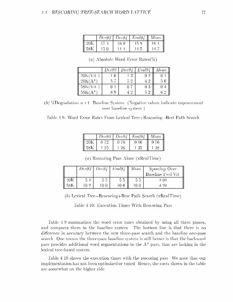
4.4. RESCORING TREE-SEARCH WORD LATTICE 77
Dev93 Dev94 Eval94 Mean
20K 17.4 16.0 15.9 16.458K 15.0 14.4 14.5 14.7
(a) Absolute Word Error Rates(%).
Dev93 Dev94 Eval94 Mean
20K(Vit.) -1.0 1.3 0.2 0.120K(A*) 5.7 5.2 4.2 5.058K(Vit.) -0.1 0.7 0.3 0.458K(A*) 8.9 4.2 5.2 6.2
(b) %Degradation w.r.t. Baseline System. (Negative values indicate improvementover baseline system.)
Table 4.9: Word Error Rates From Lexical Tree+Rescoring+Best Path Search.
Dev93 Dev94 Eval94 Mean
20K 0.72 0.76 0.80 0.7658K 1.25 1.26 1.35 1.28
(a) Rescoring Pass Alone (xRealTime).
Dev93 Dev94 Eval94 Mean Speedup OverBaseline Fwd.Vit.
20K 5.4 5.5 5.5 5.5 4.0458K 10.2 10.0 10.0 10.0 4.24
(b) Lexical Tree+Rescoring+Best Path Search (xRealTime).
Table 4.10: Execution Times With Rescoring Pass.
Table 4.9 summarizes the word error rates obtained by using all three passes,and compares them to the baseline system. The bottom line is that there is nodi�erence in accuracy between the new three-pass search and the baseline one-passsearch. One reason the three-pass baseline system is still better is that the backwardpass provides additional word segmentations to the A* pass, that are lacking in thelexical tree-based system.
Table 4.10 shows the execution times with the rescoring pass. We note that ourimplementation has not been optimized or tuned. Hence, the costs shown in the tableare somewhat on the higher side.
78 CHAPTER 4. SEARCH SPEED OPTIMIZATION
4.4.3 Summary
The main conclusion from this section is that the word lattice output of the lexicaltree is compact and has a low lattice-error rate. We are able to recover the baselinesystem recognition accuracy at the cost of about 15% increase in computation. Thecomputational overhead is less than 5% compared to the forward pass of the baselinesystem. The 3-pass tree-based recognizer is about 4.1 times faster than the forwardpass of the baseline system on our benchmarks.
We also conclude that though the tree search is sub-optimal in that the outputword segmentations are occasionally incorrect, it is possible to recover the loss usinga second rescoring pass similar to the �rst pass of the baseline Sphinx-II system. TheA* accuracy of the baseline system is still slightly better because of the additionalword segmentations provided by its backward pass.
4.5 Phonetic Fast Match
4.5.1 Motivation
We have described the senone as the acoustic model shared by a cluster of phoneticHMM states (Sections 2.1.2 and 3.1.1). Mei-Yuh Hwang in her dissertation [27]has pointed out that \: : : each senone describes a very short distinct acoustic event(shorter than a phoneme): : : ," and \: : : it can be used to construct models of all kindsof acoustic phenomena." One of the phenomena modelled by senones is the relativeactivity of the di�erent phonemes at any given time.
Let us see how senones can be used to predict the presence or absence of a givenbasephone at a given point in the input speech. In Sphinx, clusters of HMM statesthat form a senone can only belong to a single parent basephone. That is, senones arepartitioned among basephones. Consider all basephones pi; i = 1; 2; : : :. Let CD(pi)represent the collection of context dependent triphones derived from pi as well as piitself. We say that senone s � CD(pi), if s models any state of any phone in CD(pi).(Similarly, s � pi, if s models any of the states of the basephone pi.) At each timeinstant t, we compute base phone scores given by:
Ppi(t) = maxs � CD(pi)
(bs(t)); i = 1; 2; : : : (4.2)
where bs(t) is the output probability of senone s at t. That is, Ppi(t) is the outputprobability, at time t, of the best scoring senone belonging to basephone pi or anytriphone derived from it. Equation 4.2 de�nes an ordering or ranking among allbasephones, as well as the acoustic separation between them, in each frame.
We can use the above ranking as a measure of the relative activity of the individualbasephones at any point in time. The basic understanding is that if Ppi(t) >> Ppj(t)
4.5. PHONETIC FAST MATCH 79
for some two basephones pi and pj , then none of the states derived from pj will scorewell at t, and all instances of HMMs derived from pj can be pruned from search.In other words, by setting a pruning threshold or beam width relative to the bestscoring basephone, we can limit the search at time t to just those falling within thethreshold. The phones within the beamwidth at t are the list of active candidates tobe searched at t. Because of this similarity to word-level fast match techniques thatidentify candidate words active at a given time, we call this the phonetic fast matchheuristic.
The proposed heuristic raises the following issues:
� Like other fast match techniques, the phonetic fast match can cause pruningerrors during search. This occurs because senone scores are noisy, as we shallsee later in Section 4.5.2, and they occasionally mispredict the active phones.We explore e�cient ways of minimizing pruning errors later under this section.
� Equation 4.2 requires the computation of all senone output probabilities inorder to determine the base phone scores. That is relatively expensive for a fastmatch heuristic. We can also obtain base phone scores from just the contextindependent senones; i.e., s � pi instead of s � CD(pi) in equation 4.2. However,by omitting the more detailed context dependent senones from the heuristic, wemake the phone scores and ranking less reliable, and the beamwidth must beincreased to avoid pruning errors. We explore the trade-o�s presented by thesealternatives.
A somewhat similar approach to search pruning has also been suggested in [56, 31].In their work, phones are pruned from the search process based on their posteriorprobabilities estimated using neural network models. It is also di�erent in that thepruning mechanism is embedded in a hybrid Viterbi-stack decoding algorithm. Fi-nally, we use the phone prediction mechanism to activate new phones at a givenpoint in the search, and not to deactivate already active ones, unlike in their case.We believe that this leads to a more robust pruning heuristic given the nature of oursemi-continuous acoustic models.
In Section 4.5.2, we present the details of the heuristic and its incorporation as afast match front end into the lexical tree search. This description is primarily basedon equation 4.2, i.e., using all senones to compute the base phone scores. But mostof it also applies to the alternative scheme of using only the context independentsenones. We present details of the performance of both schemes on our benchmarksin Sections 4.5.3 and 4.5.4, respectively.

80 CHAPTER 4. SEARCH SPEED OPTIMIZATION
4.5.2 Details of Phonetic Fast Match
Phones Predicted by Best Scoring Senones
We �rst consider an example of the base phone ranking produced by equation 4.2.Figure 4.11 illustrates the heuristic with an example extracted from one of our bench-mark tests. Each row represents one frame of speech. All senone output probabilitiesare computed in each frame to obtain a base phone score. The base phones are rankedaccordingly and pruned with a certain threshold. We list the remaining active phonesin each frame in descending order of their scores. (See Appendix A for a completelist of the 50 context independent phones used in Sphinx-II.) The �gure underscoresseveral points:
� The candidate basephone list in each frame, even though quite short, appearsto contain the correct base phone, and quite often at the head of the list. Weemphasize appears because, a priori, it is by no means clear which base phone isthe \correct" one in any given frame. At this point we can only visually discerna pattern in the candidate lists that seems to match the expected basephonesequence fairly well.
� It is obvious that the best phone in a frame is certainly not always the correctone, whatever that may be, since we sometimes observe a best phone that isnot any of the correct ones. Hence, it is necessary to look further down the listfor the correct basephone.
� The choice of the pruning threshold is crucial. Too tight a threshold causes thecorrect phone to be pruned entirely from the list. On the other hand, if it istoo wide, we end up with too many unnecessary candidates.
� The length of the list varies from frame to frame, indicating the acoustic con-fusability within each frame. The confusion is higher around phone boundaries.
Quality of Phone Prediction
We can estimate the quality of this heuristic by measuring the position of the correctbase phone in the candidate list in each frame. But we �rst need to know what thecorrect phone is in a given frame. For that we use the Viterbi alignment [52] of thecorrect sequence of phones to the input speech10. Speci�cally, the experiment consistsof the following steps:
1. Obtain the Viterbi alignment for an entire test set. This gives us a correctbasephone mapping for each frame in the test set.
10The choice of Viterbi alignment as the reference is debatable. But we believe that any otheralignment process will not make a signi�cant di�erence to the resulting phone segmentations.
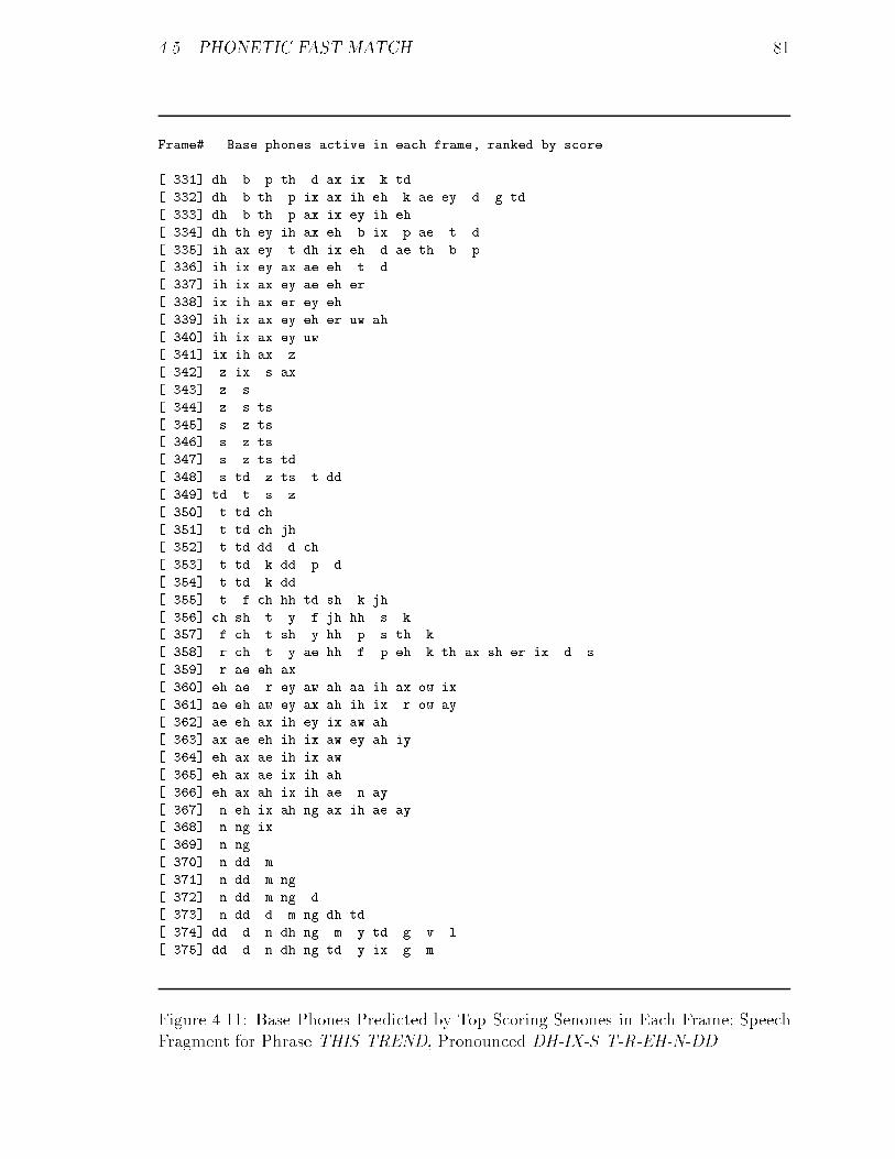
4.5. PHONETIC FAST MATCH 81
Frame# Base phones active in each frame, ranked by score
------ -----------------------------------------------------
[ 331] dh b p th d ax ix k td
[ 332] dh b th p ix ax ih eh k ae ey d g td
[ 333] dh b th p ax ix ey ih eh
[ 334] dh th ey ih ax eh b ix p ae t d
[ 335] ih ax ey t dh ix eh d ae th b p
[ 336] ih ix ey ax ae eh t d
[ 337] ih ix ax ey ae eh er
[ 338] ix ih ax er ey eh
[ 339] ih ix ax ey eh er uw ah
[ 340] ih ix ax ey uw
[ 341] ix ih ax z
[ 342] z ix s ax
[ 343] z s
[ 344] z s ts
[ 345] s z ts
[ 346] s z ts
[ 347] s z ts td
[ 348] s td z ts t dd
[ 349] td t s z
[ 350] t td ch
[ 351] t td ch jh
[ 352] t td dd d ch
[ 353] t td k dd p d
[ 354] t td k dd
[ 355] t f ch hh td sh k jh
[ 356] ch sh t y f jh hh s k
[ 357] f ch t sh y hh p s th k
[ 358] r ch t y ae hh f p eh k th ax sh er ix d s
[ 359] r ae eh ax
[ 360] eh ae r ey aw ah aa ih ax ow ix
[ 361] ae eh aw ey ax ah ih ix r ow ay
[ 362] ae eh ax ih ey ix aw ah
[ 363] ax ae eh ih ix aw ey ah iy
[ 364] eh ax ae ih ix aw
[ 365] eh ax ae ix ih ah
[ 366] eh ax ah ix ih ae n ay
[ 367] n eh ix ah ng ax ih ae ay
[ 368] n ng ix
[ 369] n ng
[ 370] n dd m
[ 371] n dd m ng
[ 372] n dd m ng d
[ 373] n dd d m ng dh td
[ 374] dd d n dh ng m y td g v l
[ 375] dd d n dh ng td y ix g m
Figure 4.11: Base Phones Predicted by Top Scoring Senones in Each Frame; SpeechFragment for Phrase THIS TREND, Pronounced DH-IX-S T-R-EH-N-DD.
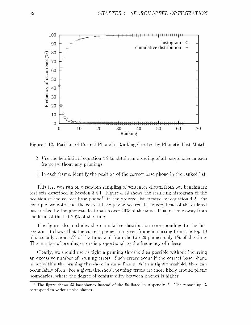
82 CHAPTER 4. SEARCH SPEED OPTIMIZATION
0
10
20
30
40
50
60
70
80
90
100
0 10 20 30 40 50 60 70
Freq
uenc
y of
occ
urre
nce(
%)
Ranking
histogramcumulative distribution
Figure 4.12: Position of Correct Phone in Ranking Created by Phonetic Fast Match.
2. Use the heuristic of equation 4.2 to obtain an ordering of all basephones in eachframe (without any pruning).
3. In each frame, identify the position of the correct base phone in the ranked list.
This test was run on a random sampling of sentences chosen from our benchmarktest sets described in Section 3.4.1. Figure 4.12 shows the resulting histogram of theposition of the correct base phone11 in the ordered list created by equation 4.2. Forexample, we note that the correct base phone occurs at the very head of the orderedlist created by the phonetic fast match over 40% of the time. It is just one away fromthe head of the list 20% of the time.
The �gure also includes the cumulative distribution corresponding to the his-togram. It shows that the correct phone in a given frame is missing from the top 10phones only about 5% of the time, and from the top 20 phones only 1% of the time.The number of pruning errors is proportional to the frequency of misses.
Clearly, we should use as tight a pruning threshold as possible without incurringan excessive number of pruning errors. Such errors occur if the correct base phoneis not within the pruning threshold in some frame. With a tight threshold, they canoccur fairly often. For a given threshold, pruning errors are more likely around phoneboundaries, where the degree of confusability between phones is higher.
11The �gure shows 63 basephones instead of the 50 listed in Appendix A. The remaining 13correspond to various noise phones.
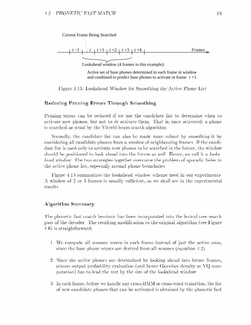
4.5. PHONETIC FAST MATCH 83
Current Frame Being Searched
Framest tt tt t−1 +2 +3 +4
Lookahead window (4 frames in this example):
Active set of base phones determined in each frame in windowand combined to predict base phones to activate in frame
+1
t +1.
Figure 4.13: Lookahead Window for Smoothing the Active Phone List.
Reducing Pruning Errors Through Smoothing
Pruning errors can be reduced if we use the candidate list to determine when toactivate new phones, but not to de-activate them. That is, once activated, a phoneis searched as usual by the Viterbi beam search algorithm.
Secondly, the candidate list can also be made more robust by smoothing it byconsidering all candidate phones from a window of neighbouring frames. If the candi-date list is used only to activate new phones to be searched in the future, the windowshould be positioned to look ahead into the future as well. Hence, we call it a looka-head window. The two strategies together overcome the problem of sporadic holes inthe active phone list, especially around phone boundaries.
Figure 4.13 summarizes the lookahead window scheme used in our experiments.A window of 2 or 3 frames is usually su�cient, as we shall see in the experimentalresults.
Algorithm Summary
The phonetic fast match heuristic has been incorporated into the lexical tree searchpass of the decoder. The resulting modi�cation to the original algorithm (see Figure4.6) is straightforward:
1. We compute all senones scores in each frame instead of just the active ones,since the base phone scores are derived from all senones (equation 4.2).
2. Since the active phones are determined by looking ahead into future frames,senone output probability evaluation (and hence Gaussian density or VQ com-putation) has to lead the rest by the size of the lookahead window.
3. In each frame, before we handle any cross-HMM or cross-word transition, the listof new candidate phones that can be activated is obtained by the phonetic fast
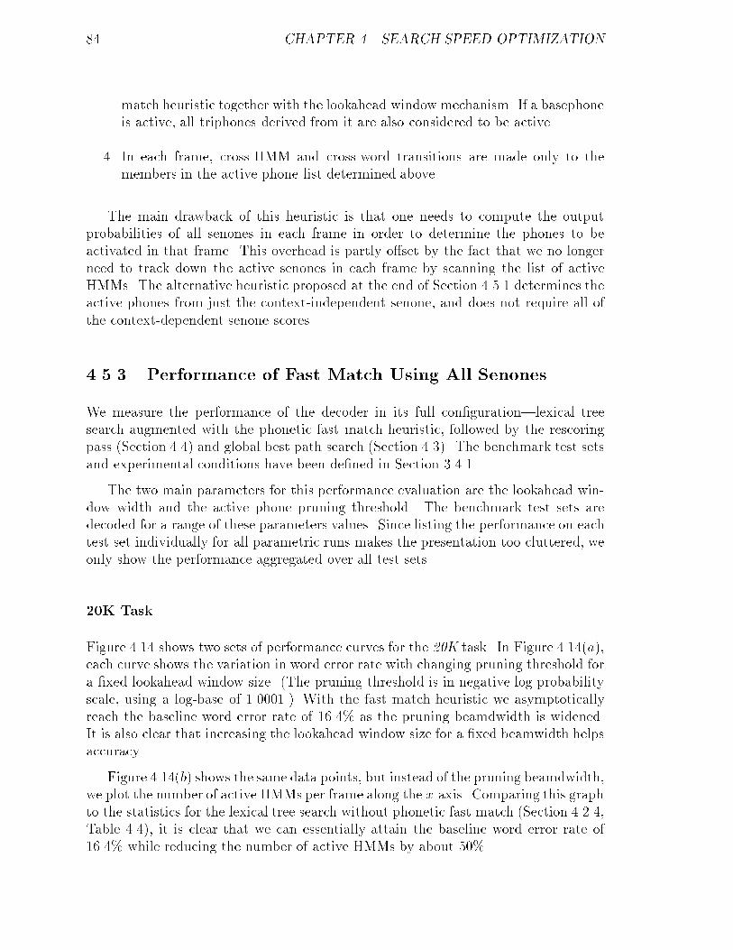
84 CHAPTER 4. SEARCH SPEED OPTIMIZATION
match heuristic together with the lookahead window mechanism. If a basephoneis active, all triphones derived from it are also considered to be active.
4. In each frame, cross-HMM and cross-word transitions are made only to themembers in the active phone list determined above.
The main drawback of this heuristic is that one needs to compute the outputprobabilities of all senones in each frame in order to determine the phones to beactivated in that frame. This overhead is partly o�set by the fact that we no longerneed to track down the active senones in each frame by scanning the list of activeHMMs. The alternative heuristic proposed at the end of Section 4.5.1 determines theactive phones from just the context-independent senone, and does not require all ofthe context-dependent senone scores.
4.5.3 Performance of Fast Match Using All Senones
We measure the performance of the decoder in its full con�guration|lexical treesearch augmented with the phonetic fast match heuristic, followed by the rescoringpass (Section 4.4) and global best path search (Section 4.3). The benchmark test setsand experimental conditions have been de�ned in Section 3.4.1.
The two main parameters for this performance evaluation are the lookahead win-dow width and the active phone pruning threshold. The benchmark test sets aredecoded for a range of these parameters values. Since listing the performance on eachtest set individually for all parametric runs makes the presentation too cluttered, weonly show the performance aggregated over all test sets.
20K Task
Figure 4.14 shows two sets of performance curves for the 20K task. In Figure 4.14(a),each curve shows the variation in word error rate with changing pruning threshold fora �xed lookahead window size. (The pruning threshold is in negative log-probabilityscale, using a log-base of 1.0001.) With the fast match heuristic we asymptoticallyreach the baseline word error rate of 16.4% as the pruning beamdwidth is widened.It is also clear that increasing the lookahead window size for a �xed beamwidth helpsaccuracy.
Figure 4.14(b) shows the same data points, but instead of the pruning beamdwidth,we plot the number of active HMMs per frame along the x-axis. Comparing this graphto the statistics for the lexical tree search without phonetic fast match (Section 4.2.4,Table 4.4), it is clear that we can essentially attain the baseline word error rate of16.4% while reducing the number of active HMMs by about 50%.
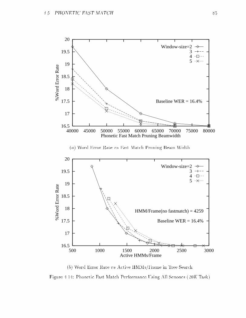
4.5. PHONETIC FAST MATCH 85
16.5
17
17.5
18
18.5
19
19.5
20
40000 45000 50000 55000 60000 65000 70000 75000 80000
%W
ord
Err
or R
ate
Phonetic Fast Match Pruning Beamwidth
Baseline WER = 16.4%
Window-size=2345
(a) Word Error Rate vs Fast Match Pruning Beam Width.
16.5
17
17.5
18
18.5
19
19.5
20
500 1000 1500 2000 2500 3000
%W
ord
Err
or R
ate
Active HMMs/Frame
Baseline WER = 16.4%
HMM/Frame(no fastmatch) = 4259
Window-size=2345
(b) Word Error Rate vs Active HMMs/Frame in Tree Search.
Figure 4.14: Phonetic Fast Match Performance Using All Senones (20K Task).
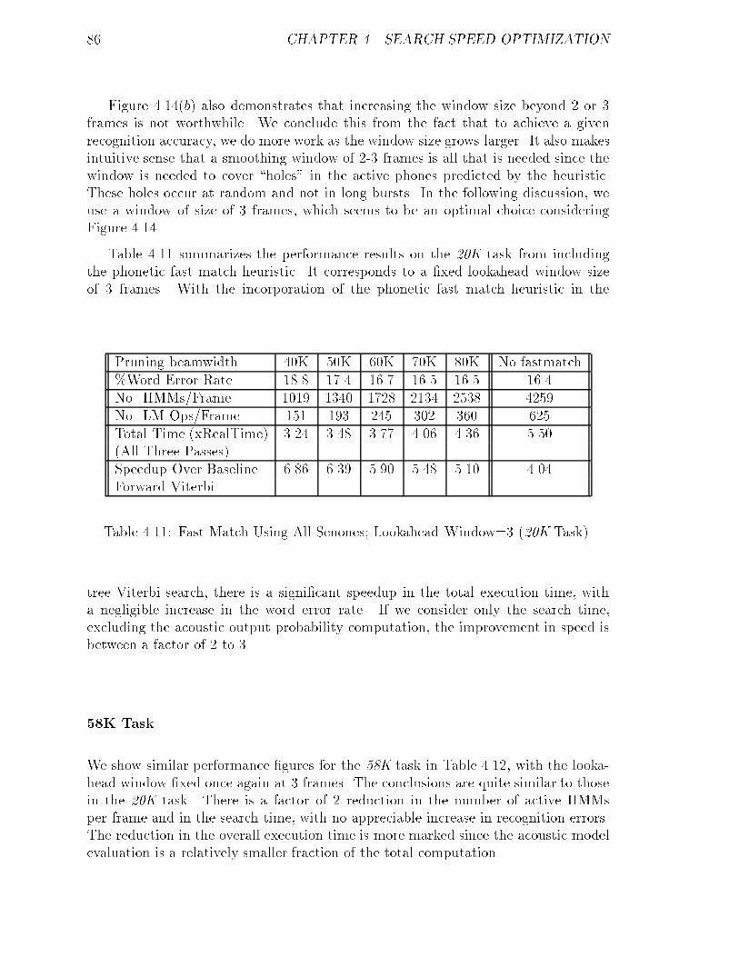
86 CHAPTER 4. SEARCH SPEED OPTIMIZATION
Figure 4.14(b) also demonstrates that increasing the window size beyond 2 or 3frames is not worthwhile. We conclude this from the fact that to achieve a givenrecognition accuracy, we do more work as the window size grows larger. It also makesintuitive sense that a smoothing window of 2-3 frames is all that is needed since thewindow is needed to cover \holes" in the active phones predicted by the heuristic.These holes occur at random and not in long bursts. In the following discussion, weuse a window of size of 3 frames, which seems to be an optimal choice consideringFigure 4.14.
Table 4.11 summarizes the performance results on the 20K task from includingthe phonetic fast match heuristic. It corresponds to a �xed lookahead window sizeof 3 frames. With the incorporation of the phonetic fast match heuristic in the
Pruning beamwidth 40K 50K 60K 70K 80K No fastmatch%Word Error Rate 18.8 17.4 16.7 16.5 16.5 16.4No. HMMs/Frame 1019 1340 1728 2134 2538 4259No. LM Ops/Frame 151 193 245 302 360 625Total Time (xRealTime) 3.24 3.48 3.77 4.06 4.36 5.50(All Three Passes)Speedup Over Baseline 6.86 6.39 5.90 5.48 5.10 4.04Forward Viterbi
Table 4.11: Fast Match Using All Senones; Lookahead Window=3 (20K Task).
tree Viterbi search, there is a signi�cant speedup in the total execution time, witha negligible increase in the word error rate. If we consider only the search time,excluding the acoustic output probability computation, the improvement in speed isbetween a factor of 2 to 3.
58K Task
We show similar performance �gures for the 58K task in Table 4.12, with the looka-head window �xed once again at 3 frames. The conclusions are quite similar to thosein the 20K task. There is a factor of 2 reduction in the number of active HMMsper frame and in the search time, with no appreciable increase in recognition errors.The reduction in the overall execution time is more marked since the acoustic modelevaluation is a relatively smaller fraction of the total computation.
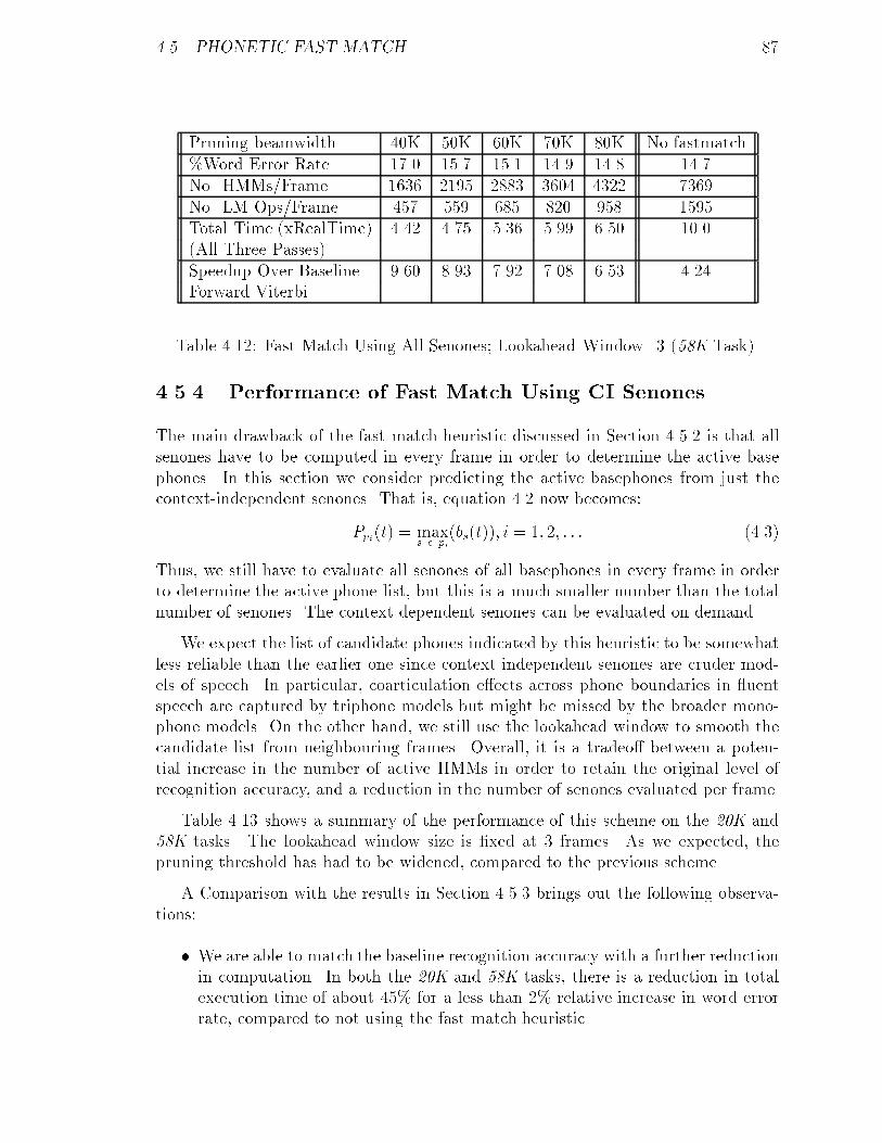
4.5. PHONETIC FAST MATCH 87
Pruning beamwidth 40K 50K 60K 70K 80K No fastmatch%Word Error Rate 17.0 15.7 15.1 14.9 14.8 14.7No. HMMs/Frame 1636 2195 2883 3604 4322 7369No. LM Ops/Frame 457 559 685 820 958 1595Total Time (xRealTime) 4.42 4.75 5.36 5.99 6.50 10.0(All Three Passes)Speedup Over Baseline 9.60 8.93 7.92 7.08 6.53 4.24Forward Viterbi
Table 4.12: Fast Match Using All Senones; Lookahead Window=3 (58K Task).
4.5.4 Performance of Fast Match Using CI Senones
The main drawback of the fast match heuristic discussed in Section 4.5.2 is that allsenones have to be computed in every frame in order to determine the active basephones. In this section we consider predicting the active basephones from just thecontext-independent senones. That is, equation 4.2 now becomes:
Ppi(t) = maxs � pi
(bs(t)); i = 1; 2; : : : (4.3)
Thus, we still have to evaluate all senones of all basephones in every frame in orderto determine the active phone list, but this is a much smaller number than the totalnumber of senones. The context dependent senones can be evaluated on demand.
We expect the list of candidate phones indicated by this heuristic to be somewhatless reliable than the earlier one since context independent senones are cruder mod-els of speech. In particular, coarticulation e�ects across phone boundaries in uentspeech are captured by triphone models but might be missed by the broader mono-phone models. On the other hand, we still use the lookahead window to smooth thecandidate list from neighbouring frames. Overall, it is a tradeo� between a poten-tial increase in the number of active HMMs in order to retain the original level ofrecognition accuracy, and a reduction in the number of senones evaluated per frame.
Table 4.13 shows a summary of the performance of this scheme on the 20K and58K tasks. The lookahead window size is �xed at 3 frames. As we expected, thepruning threshold has had to be widened, compared to the previous scheme.
A Comparison with the results in Section 4.5.3 brings out the following observa-tions:
� We are able to match the baseline recognition accuracy with a further reductionin computation. In both the 20K and 58K tasks, there is a reduction in totalexecution time of about 45% for a less than 2% relative increase in word errorrate, compared to not using the fast match heuristic.

88 CHAPTER 4. SEARCH SPEED OPTIMIZATION
Pruning beamwidth 65K 75K 85K 95K 105K No fastmatch%Word Error Rate 18.1 17.1 16.7 16.6 16.5 16.4No. HMMs/Frame 1402 1707 2016 2290 2580 4259Total Time (xRealTime) 2.41 2.72 3.02 3.29 3.55 5.50(All Three Passes)Speedup Over Baseline 9.23 8.18 7.36 6.76 6.26 4.04Forward Viterbi
(a) 20K Task.
Pruning beamwidth 65K 75K 85K 95K 105K No fastmatch%Word Error Rate 16.6 15.6 15.1 14.9 14.8 14.7No. HMMs/Frame 2334 2878 3430 3919 4438 7369Total Time (xRealTime) 4.20 4.82 5.45 5.84 6.58 10.0(All Three Passes)Speedup Over Baseline 10.1 8.80 7.79 7.27 6.45 4.24Forward Viterbi
(b) 58K Task.
Table 4.13: Fast Match Using CI Senones; Lookahead Window=3.
� There is some increase in the number of active HMMs needed to achieve thesame recognition accuracy, compared to the fast match based on all senones.But it is partially o�set by the reduction in the number of senones evaluated.The balance, of course, depends on the relative costs of the two.
� Using context independent senones for the fast match is more bene�cial to thesmaller vocabulary system. As vocabulary size increases, the increase in thenumber of active HMMs a�ects larger vocabulary systems more. The reductionin the cost of computing senone output probabilities is o�set by the need toscan the active HMMs to �nd the active senones in each frame.
4.5.5 Phonetic Fast Match Summary
The conclusion is that using the phonetic fast match heuristic, the speed of the lexicaltree decoder can be improved by almost a factor of two, with negligible increase inrecognition errors. The heuristic can be further tuned in ways that we have notexplored. For example, one can use basephone-speci�c pruning beamwidths. Thegraph in Figure 4.12 is averaged over all 50 phones in the Sphinx-II system. However,certain base phones, such as fricatives and long vowels, are predicted much betterthan others. It is possible to tighten the pruning threshold for these phones.

4.6. EXPLOITING CONCURRENCY 89
The phonetic fast match also has several other potential uses. These need to beexplored:
� The active base phones usually occur clustered in time. One can create a phonelattice in which each node is a phone that is active for some contiguous set offrames. Such a phoneme lattice could be searched very e�ciently for producinga candidate list of active words to be searched.
� A phone lattice such as described above can be used for word spotting. We mayconsider the word to be present if we can trace a sequence of nodes through thephone lattice corresponding to the word's pronunciation.
� Obtaining con�dence measures. Wherever the phone lattice is sparse, i.e., veryfew phones are identi�ed as being active, we can conclude that we have a highdegree of con�dence about which phones are active. If a region of frames hasmany phones active in it, on the other hand, it indicates a high degree of acousticconfusion in that region. The acoustic modelling in that segment is less reliable.
The technique of identifying active phones has been discussed in [22], however,only in the context of applying it to a fast match. They have reported a reductionin fast-match computation of about 50% with a slightly under 10% increase in errorrate. A similar technique using phone posterior probabilities has also been reportedin [56]. It is also in the phase of the fastmatch step that generates word candidatesand posterior probabilities to a stack-decoding algorithm. The phonetic HMM statesare modelled by neural network that directly estimate phone posterior probabilitiesthat are used to identify and deactivate inactive phones during the fast match step.They report an order of magnitude increase in search speed for a nearly real-timeperformance, while incurring a 7% relative increase in word error rate on a 20K task.Part of the large increase in speed in probably owing to the fact that the basic decoderis based on stack-decoding algorithm. They do not report frequency counts for thereduction in the number of active models per frame.
4.6 Exploiting Concurrency
Our main purpose in this section is to explore the potential for speeding up the recog-nition architecture via concurrency. It is relevant since modern commercial processorarchitectures are increasingly capable of multiprocessor operation and commercial op-erating systems support concurrency and multithreading within single applications.It is possible to take good advantage of this facility.
One of the early attempts at speeding up the Sphinx-II baseline system exploitedthe large degree of concurrency within its algorithmic steps [54]. In a parallel imple-mentation on the PLUS multiprocessor designed at CMU [13], a speed up of 3.9 was

90 CHAPTER 4. SEARCH SPEED OPTIMIZATION
obtained on a 5 node con�guration. The parallelization involved static partitioningof data and computation among multiple threads using the Mach C-threads facility[16]. Though the lexical tree decoder has signi�cant structural di�erences comparedto the baseline system, some of the parallelization techniques can still be applied toit. We explore this question in some detail in this section.
In parallelizing any application, there are two broad options: dynamic load bal-ancing using a central task queue model, or static load balancing based on somesuitable static data and computation partitioning. The former presumably achievesthe best (most even) load balance among the active threads. But it is more complexto implement, and harder to maintain and modify for experimentation purposes. Weconsider static partitioning schemes which are easier to manipulate in a coarse-grainedfashion on small-scale multiprocessors.
In the following discussion we assume a shared-memory multiprocessor con�gu-ration with an application running in a single address space shared by multiple con-current threads. The discussion is hypothetical. We have not actually implementeda parallel version of the tree search decoder. But we do address the relevant issues.
4.6.1 Multiple Levels of Concurrency
There are several levels of concurrency in the decoder as discussed so far, which canbe exploited individually and in combination. We review the main ones brie y.
Pipelining Between Search Passes
The lexical tree search and rescoring passes can be pipelined and executed concur-rently. If the latter is time synchronous, the only constraint is that it cannot proceedbeyond time t until the lexical tree search has completed emitting all its word latticeentries that correspond to a begin time of t or earlier. This is easily established bychecking the history information Hm
j in each active HMM (see Section 3.2.4). If allof them point to word lattice entries with end times greater than t, the rescoring passcan proceed beyond t12.
The potential speedup obviously depends on the relative costs of the two passes.In our benchmark system, the lexical tree search is the dominant pass. However, itcan be parallelized internally, so pipelining the later pass becomes useful.
The communication bandwidth between the two passes is minimal. It only involvesthe exchange of word lattice information, which consists of a few tens of words everyframe, on average. The two passes must also synchronize to ensure that the rescoringpass does not overtake the other.
12Actually, the rescoring pass treats the word segmentations in the tree search word lattice fuzzily,using a window, as described in Section 4.4.1. We must also allow for the window.

4.6. EXPLOITING CONCURRENCY 91
Pipelining Between Acoustic and HMM Evaluation in Tree Search
We can pipeline the VQ and senone output probability computation with the HMMsearch if there is no feedback from the latter to the former. That is the case if wedecide to evaluate all senones every frame, instead of computing just the active ones.The latter requires feedback from the active HMMs. The phonetic fast match heuristicpresented in Section 4.5.2 requires the evaluation of all senone output probabilitiesevery frame anyway. Hence this pipelining is suitable in that context.
Again, the potential speedup depends on the costs of the individual steps. Inour lexical tree search using semi-continuous acoustic models, the execution timesfor senone output probability computation and searching the active HMMs are fairlyeven for the 20K task. This is seen from Tables 4.3(a) and 4.11. Even otherwise,each component has a fair amount of internal parallelism which can be exploited tobalance the computation.
We consider the communication bandwidth between the two components. Thedata exchanged between the pipeline components consists of the senone output prob-abilities in each frame. In our system, it amounts to 10K 4-byte values in each frame,or about 4MB/sec, and it is not likely to be signi�cantly di�erent for most systems.This volume is well within the capabilities of modern memory-bus systems.
The two pipeline components have a producer-consumer relationship. The pro-ducer, senone evaluation, must stay ahead of the consumer, the search component.The execution time for the former is fairly constant from frame to frame, but thesearch cost can vary by an order of magnitude or more. Hence, for a proper balancein computation, the two cannot be simply run in lockstep. We need a queue of framesbetween the two to smooth out variations in execution times. However, the queuecannot be arbitrarily large since it has to contain 40KB of senone output probabilitydata per frame. We surmise that a queue depth of about 10 frames is su�cient tokeep the pipeline owing relatively smoothly without hiccups.
Partitioning Acoustic Output Probability Computation
The computation of senone output probabilities can be trivially partitioned in mostinstances. Basically, there is no dependency between the output probabilities ofdi�erent senones within a given frame. Every senone can be evaluated concurrentlywith the others.
Partitioning the senone output probability computation creates a multiple-producerand consumer relationship with the search module. Hence the latter must synchronizewith all of the producer partitions to ensure integrity.
92 CHAPTER 4. SEARCH SPEED OPTIMIZATION
Concurrency in Searching the Lexical Tree HMM Network
Parallelism inside the Viterbi tree search algorithm is the hardest to control andexploit e�ectively for several reasons:
� The beam search heuristic restricts the active HMMs to a small fraction of thetotal number. The actual identity of the active HMMs is time varying. It isnecessary to balance the computation among parallel components in spite ofthis variation.
� The amount of search computation varies by orders of magnitude from frameto frame.
� There is global dependency from one frame to the next. This follows fromthe time-synchronous nature of the Viterbi algorithm. For example, the wordlattice must be completely updated with new word entries in a given framebefore moving on to attempt cross-word transitions in that frame.
� The search component is the most memory intensive. The memory access pat-tern is highly unstructured since the set of active HMMs varies over time. Thememory bottleneck is probably the largest impediment to the e�ective paral-lelization of this component.
The most natural way to parallelize the lexical tree search is by partitioning thecollection of trees among concurrent threads. For example, the two trees in Figure4.2 can be assigned to separate threads. This approach has the following advantages:
� The computation within each thread is largely the same as in the sequentialalgorithm. It is important to retain the simplicity of structure o�ered by se-quential implementations for ease of modi�cation and experimentation. Themain di�erence is that threads need to synchronize with each other once ineach frame to exchange updates to the word lattice.
� Since the HMM data structures to be searched are partitioned, there is nocon ict during access to them, except for cross-word transition updates. Theseare handled by exchanging updates to the word lattice as mentioned above.
� The large number of trees o�er su�cient parallelism and scope for e�ectiveload balancing in spite of the level of activity within individual trees varyingsubstantially with time. In the 20K task, there are about 650 trees (see Table4.1).
It is important to distribute the trees with some care, in order to maintain aproper load balance among threads. The phonetic fast match heuristic restricts theactivity at the root nodes by allowing only the predicted phones to become active at
4.7. SUMMARY OF SEARCH SPEED OPTIMIZATION 93
a given point in time. Hence, it is advantageous to scatter trees with root nodes thathave the same parent basephone among di�erent threads. In general, it is desirableto spread trees with acoustically similar initial pre�xes among threads, ensuring amore even distribution of the computation load.
4.6.2 Parallelization Summary
We have reviewed the potential for speedup through parallelism at several levels.Even with a static partitioning of the task, the available concurrency can be e�ectivelyexploited on small-scale shared-memory multiprocessors.
It is possible to pipeline individual passes of the decoder with one another. Withinthe lexical tree search, we can exploit pipelining between the acoustic output prob-ability evaluation for senones and the HMM search algorithm. This is especiallyadvantageous since they are fairly evenly matched in our lexical tree decoder usingsemi-continuous models. Finally, both acoustic output probability computation andHMM search can be partitioned into concurrent threads. However, the latter requiresa careful static assignment of the overall search space to threads in order to balancethe computational load among them.
However, the e�ectiveness of a parallel implementation is limited by the availableprocessor-memory bandwidth. Since certain portions of the original sequential algo-rithm, especially HMM evaluation, are heavily memory bound, the actual speeduppossible through concurrency remains to be seen.
4.7 Summary of Search Speed Optimization
The contents of this chapter can be summarized by comparing the performances ofvarious approaches along two axes: word error rate vs recognition speed. Figure 4.15captures this information succinctly.
The �gure shows that we can very nearly attain the recognition accuracy of thebaseline system while speeding up the system by a factor of about 8. It also bringsout the relative contributions and costs of each technique. Appendix B contains asummary of the results of signi�cance tests on the di�erences between the recognitionaccuracies of the various systems.
We brie y review the results from this chapter:
� The lexical tree search algorithm is about 5 times faster than the baselineSphinx-II system. The search component alone, excluding the computation ofacoustic output probabilities of senones, is over 7 times faster than the baselinesystem.
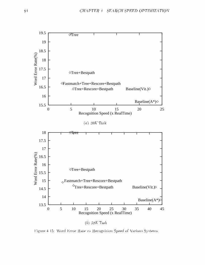
94 CHAPTER 4. SEARCH SPEED OPTIMIZATION
15.5
16
16.5
17
17.5
18
18.5
19
19.5
0 5 10 15 20 25
Wor
d E
rror
Rat
e(%
)
Recognition Speed (x RealTime)
Baseline(Vit.)
Baseline(A*)
Tree
Tree+Bestpath
Tree+Rescore+BestpathFastmatch+Tree+Rescore+Bestpath
(a) 20K Task.
13.5
14
14.5
15
15.5
16
16.5
17
17.5
18
0 5 10 15 20 25 30 35 40 45
Wor
d E
rror
Rat
e(%
)
Recognition Speed (x RealTime)
Baseline(Vit.)
Baseline(A*)
Tree
Tree+Bestpath
Tree+Rescore+Bestpath
Fastmatch+Tree+Rescore+Bestpath
(b) 58K Task.
Figure 4.15: Word Error Rate vs Recognition Speed of Various Systems.
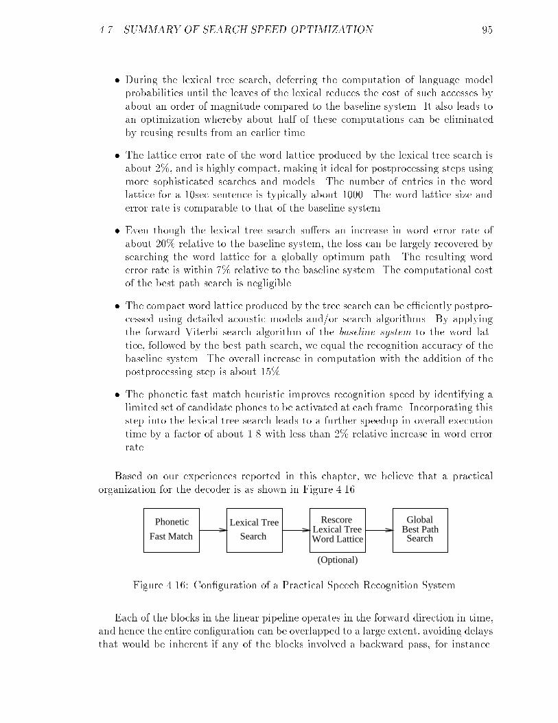
4.7. SUMMARY OF SEARCH SPEED OPTIMIZATION 95
� During the lexical tree search, deferring the computation of language modelprobabilities until the leaves of the lexical reduces the cost of such accesses byabout an order of magnitude compared to the baseline system. It also leads toan optimization whereby about half of these computations can be eliminatedby reusing results from an earlier time.
� The lattice error rate of the word lattice produced by the lexical tree search isabout 2%, and is highly compact, making it ideal for postprocessing steps usingmore sophisticated searches and models. The number of entries in the wordlattice for a 10sec sentence is typically about 1000. The word lattice size anderror rate is comparable to that of the baseline system.
� Even though the lexical tree search su�ers an increase in word error rate ofabout 20% relative to the baseline system, the loss can be largely recovered bysearching the word lattice for a globally optimum path. The resulting worderror rate is within 7% relative to the baseline system. The computational costof the best path search is negligible.
� The compact word lattice produced by the tree search can be e�ciently postpro-cessed using detailed acoustic models and/or search algorithms. By applyingthe forward Viterbi search algorithm of the baseline system to the word lat-tice, followed by the best path search, we equal the recognition accuracy of thebaseline system. The overall increase in computation with the addition of thepostprocessing step is about 15%.
� The phonetic fast match heuristic improves recognition speed by identifying alimited set of candidate phones to be activated at each frame. Incorporating thisstep into the lexical tree search leads to a further speedup in overall executiontime by a factor of about 1.8 with less than 2% relative increase in word errorrate.
Based on our experiences reported in this chapter, we believe that a practicalorganization for the decoder is as shown in Figure 4.16.
Phonetic
Fast Match
Lexical Tree
Search
RescoreLexical TreeWord Lattice
GlobalBest PathSearch
(Optional)
Figure 4.16: Con�guration of a Practical Speech Recognition System.
Each of the blocks in the linear pipeline operates in the forward direction in time,and hence the entire con�guration can be overlapped to a large extent, avoiding delaysthat would be inherent if any of the blocks involved a backward pass, for instance.
96 CHAPTER 4. SEARCH SPEED OPTIMIZATION
The lexical tree search module, using fairly detailed acoustic and grammar modelsbut simple enough to allow near real-time operation, produces a compact word latticewith a low lattice error rate. It is the key to the overall organization of a practicalspeech recognition system.
Additional improvements in speed can be obtained by exploiting parallelism be-tween and within the individual blocks in Figure 4.16. The pipelined organizationlends itself naturally to a parallel implementation, operating asynchronously in adata-driven fashion. There is also a large amount of parallelism within some of themodules. For example, the evaluation of acoustic models and the HMM networksearch can be performed in parallel, with very simple communication between them.One of the early work in this area was in parallelizing the forward Viterbi pass ofthe baseline Sphinx-II system on a 5-node shared-memory multiprocessor [14, 13] onthe 1000-word Resource Management task [51], which yielded a speedup of about 3.8[54]. Parallelizing the lexical tree search is a little di�erent, but the potential exists,nevertheless.

Chapter 5
Memory Size Reduction
The second important computational resource needed by modern speech recognitionsystems, after CPU power, is main memory size. Most research systems requirehundreds of megabytes of main memory that are only found on high-end workstations.Clearly, practical applications of speech recognition must be able to run on muchsmaller memory con�gurations.
The work reported in this chapter is once again in the context of the baselineSphinx-II system described in Chapter 3. It is typical of most other research systemsin use in the speech community. The two main candidates for memory usage inthe baseline Sphinx-II system are the acoustic and language models. The formeris dominated by the senone mixture weights (see Sections 2.1.2, 3.1.1, and 3.4.4).The latter primarily consists of the bigram and trigram data structures described inSection 3.4.4, Figure 3.8.
In this chapter we describe the approaches taken to reduce their sizes in the lexicaltree decoder. In Section 5.1 we discuss the reduction of acoustic model size and inSection 5.2 that of the language model. Some of the techniques presented here havealso been incorporated into the baseline decoder with similar results.
5.1 Senone Mixture Weights Compression
The main hypothesis in designing a scheme for reducing the memory size requirementof acoustic models is that the exact state score (or senone score) in each frame is not asimportant to the detailed search as is the relative ranking of the models. Furthermore,short-term �ne distinctions in the scores of states in a given frame are misleading,because of the inherent uncertainty in the statistical models underlying those states.These observations lead to the simple solution of clustering acoustic modelling valuesinto a small number of bins which can be indirectly addressed using a small numberof bits.
97
98 CHAPTER 5. MEMORY SIZE REDUCTION
This approach is applied to the Sphinx-II semi-continuous acoustic models in thecase of the senone weights. As we saw in Section 3.4.4, the senone mixture weightsor coe�cients account for about 40MB of memory usage, where each coe�cient is a4-byte value. These coe�cients are reduced to 1 byte by simply truncating their leastsigni�cant bits until the entire dynamic range can be �t into 8 bits. Thus, we obtaina 4-fold reduction in their memory requirement.
Most benchmark evaluations described in this thesis have been carried out withthis memory organization. The impact of this truncation on recognition accuracy isvirtually non-existent. More important, only about 1% of the individual sentenceshave di�erent recognition results in the two cases. In other words, the reduction inprecision makes little di�erence not just on average, but even in detail. In fact, theoverall recognition accuracy is actually slightly better after the truncation.
There is also an execution speed bene�t to this compaction. Equation 2.1 inSection 2.1.2 de�nes the expression for the output probability of a senone in a givenframe. In Sphinx-II, as in many other speech recognition systems, all probabilitycalculations are carried out in log-space, so that multiplication operations can bereduced to additions in log-space. But the summation term in equation 2.1 poses adi�culty. By truncating all log-probability values to 8-bits, however, the additionoperation can be achieved in log-space by simply implementing it as a table-lookupoperation. This optimization reduces the execution time for senone output probabilitycomputation by a factor of 2.
5.2 Disk-Based Language Models
In the case of the language model, a totally di�erent approach is necessary. It isindeed feasible to reduce the probability values and backo� weights to 8-bit valueswithout any e�ect on recognition accuracy. But in this case, the probability valueshave already been compacted to 16-bits as mentioned in Section 3.4.4. Hence, thepayo� in reducing them to 8 bits is less. Furthermore, there are other �elds in eachbigram and trigram, such as the word-id, which are much harder to compress further.
The observation in this case is that in decoding any given utterance, only a verysmall portion of the language model is actually used. Hence, we can consider main-taining the language model entirely on disk, and retrieving only the necessary pieces,on demand. One would expect the virtual memory system to e�ectively accomplishthis for free. But, as we noted in Section 3.4.4, the granularity of access to the bi-gram and trigram data structures is much smaller than a physical page size on mostmodern workstations. For example, the average number of bigrams per word in thecase of the 58K vocabulary is about 105. The average number of trigrams per wordpair is at least an order of magnitude smaller. Hence, the virtual memory system isrelatively ine�ective in managing the working set for these data structures.
5.2. DISK-BASED LANGUAGE MODELS 99
It is possible to maintain the language model on disk and explicitly load thenecessary bigrams and trigrams on demand. However, to avoid excessive delays dueto disk access, we must resort to some caching strategy. For this, we observe thatif we are required to compute a bigram probability P (wjjwi) during some frame, weare very likely to have to compute other bigram probabilities P (wkjwi); k 6= j, in thesame frame. We can make a similar case for trigram probabilities. The reason forthis phenomenon is that typically several words arrive at their ends in a given frame,and we need to compute each of their language model probabilities with respect toeach of some set of predecessor words.
The caching policy implemented in our system is quite straightforward:
� Since unigrams are a small portion of the large vocabulary language models,they are always kept in memory. Only bigrams and trigrams are read from disk,and they are cached in logical chunks. That is, all bigram followers of a wordor all trigram followers of a word pair are cached at a time.
� Whenever a bigram probability P (wjjwi) is needed, and it is not in memory, allbigram followers of wi are read from disk and cached into memory.
� Likewise, whenever a trigram probability P (wkjwi; wj) is needed, and it is not inmemory, all trigram followers of wi; wj are read and cached in memory. Further-more, all bigram followers of wi are also read from disk and cached in memory,if not already there.
� To avoid a continual growth in the amount of cached language model data, it isnecessary to garbage collect them periodically. Since the decoder processes inputspeech one sentence at a time (which are at the most a few tens of seconds long),the cached data are ushed as follows. At the end of each utterance, we simplyfree the memory space for those cached entries which were not accessed duringthe utterance. This ensures that we recycle the memory occupied by relativelyrare words, but retain copies of frequently occurring words such as functionwords (A, THE, IS, etc.). The \cache lines" associated with the functions wordsare also relatively large, and hence more expensive to read from disk.
All the benchmark evaluations with the lexical tree decoder have been carriedout using the disk-based language model with the above caching scheme. We havemeasured the number of bigrams and trigrams resident in memory during all of ourbenchmark evaluations. In both the 20K and 58K tasks, only about 15-25% of bigramsand about 2-5% of all trigrams are resident in memory on average, depending on theutterance.
The impact of the disk-based language model on elapsed time is minimal, implyingthat the caching scheme is highly e�ective in avoiding disk access latency. Measuringelapsed time is tricky because it is a�ected by factors beyond our control, such as other
100 CHAPTER 5. MEMORY SIZE REDUCTION
processes contending for the CPU, and network delays. However, on at least someexperimental runs on entire benchmark test sets, the di�erence between the CPUusage and elapsed time is no more than if the entire language model is completelymemory-resident. The elapsed time exceeds the CPU usage by less than 5%, and itis the existence proof for the e�ectiveness of the caching policy.
5.3 Summary of Experiments on Memory Size
We have presented two simple schemes for reducing the memory sizes of large acousticand language models, respectively. The former is compressed by simply truncatingthe representation from 32 to 8 bits. This granularity appears to be quite su�cientin terms of retaining the original recognition accuracy, sentence for sentence.
The memory-resident size of the language model is reduced by maintaining iton disk, with an e�ective caching policy for eliminating disk access latency. Thefraction of bigrams in memory is reduced by a factor of between 4 and 6, and that oftrigrams by a factor of almost 20-50. Clearly, there is no question of loss of recognitionaccuracy, since there is no change in the data representation.
We believe that several other implementations use 8-bit representations for acous-tic models, although the literature hasn't discussed their e�ect on recognition, toour knowledge. We do not know of any work dealing with the language model inthe way described here. Other approaches for reducing the size of language modelsinclude various forms of clustering, for example into class-based language models,and eliminating potentially useless bigrams and trigrams from the model [58]. Theseapproaches generally su�er from some loss of accuracy. The advantage of simple wordbigram and trigram grammars is that they are easy to generate from large volumesof training data.
Chapter 6
Small Vocabulary Systems
6.1 General Issues
Although we have mainly concentrated on large vocabulary speech recognition inthis thesis, it is interesting to consider how the techniques developed here extendto smaller vocabulary tasks. There are two cases: tiny vocabulary tasks of a fewtens to a hundred words, and medium vocabulary of a few thousands of words. Theformer are typical of command and control type applications with highly constrainedvocabularies. The latter are representative of applications in constrained domains,such as queries to a �nancial database system.
For a really small vocabulary of a few tens of words, search complexity is not amajor issue. In a Viterbi beam search implementation, at most a few hundred HMMsmay be active during each frame. Similarly there may be at most a few hundredcross-word transitions. (These are the two most prominent subcomponents of searchin large vocabulary recognition, and our main focus.) The acoustic output probabilitycomputation, and questions of recognition accuracy are much more dominant issuesin such small vocabulary tasks. The nature of the problem also allows the use of adhoc techniques, such as word HMM models for improving recognition accuracy. Thewide range of options in the extremely small vocabulary domain makes the e�ciencymeasures for large vocabulary recognition less relevant.
Secondly, as the vocabulary size decreases, words tend to have fewer commonpronunciation pre�xes. For example, the triphone lexical tree for the digits lexiconin Section 3.1.2 is not a tree at all. It is completely at. The tree structure is largelyirrelevant in such cases. We do not consider extremely small vocabulary tasks anyfurther.
Even when the vocabulary is increased to a few thousands of words, the cost ofsearch does not dominate as in the case of large vocabulary tasks. The computationof HMM state output probabilities is about equally costly. Hence, even an in�nite
101
102 CHAPTER 6. SMALL VOCABULARY SYSTEMS
speedup of the search algorithm produces an overall speedup of only a small factor.
In this chapter we compare the baseline Sphinx-II system and the lexical treesearch system on the speech recognition component of the ATIS (Airline Travel In-formation Service) task1 [45, 46], which has a vocabulary of about 3K words.
Section 6.2 contains the details of the performance of the baseline Sphinx-II systemand the lexical tree decoder on the ATIS task.
6.2 Performance on ATIS
6.2.1 Baseline System Performance
ATIS is a small-vocabulary task in which the utterances are mainly queries to anair travel database regarding ight and other travel-related information. The testconditions for the ATIS task are as follows:
� 3000 word vocabulary, including several compound words, such as I_WANT,WHAT_IS, etc.
� 10,000 senone semi-continuous acoustic models trained for ATIS from both thelarge vocabulary Wall Street Journal and ATIS data.
� Word bigram language model, with about 560,000 bigrams. It is a fairly con-strained grammar with a much lower perplexity than the large vocabulary ones.
� Test set consisting of 1001 sentences, 9075 words.
The style of speaking in ATIS is a little more conversational than in the large vocab-ulary test sets from the previous chapters.
The performance of the baseline Sphinx-II system on the ATIS task is summarizedin Table 6.1. The noteworthy aspects of this test are the following (we focus mainlyon the forward Viterbi pass):
� The cost of output probability computation (VQ and senone evaluation) isalmost half of the total execution time of the forward Viterbi search. Hencespeeding up the other half, i.e. search alone, by an order of magnitude hasmuch less impact on the overall speed.
� The number of HMMs evaluated per frame is still su�ciently large that it isnot worth while computing the senone output probabilities on demand. It isless expensive to compute all of them in each frame.
1The overall ATIS task has other components to it, such as natural language understanding ofthe spoken sentence. We ignore them in this discussion.
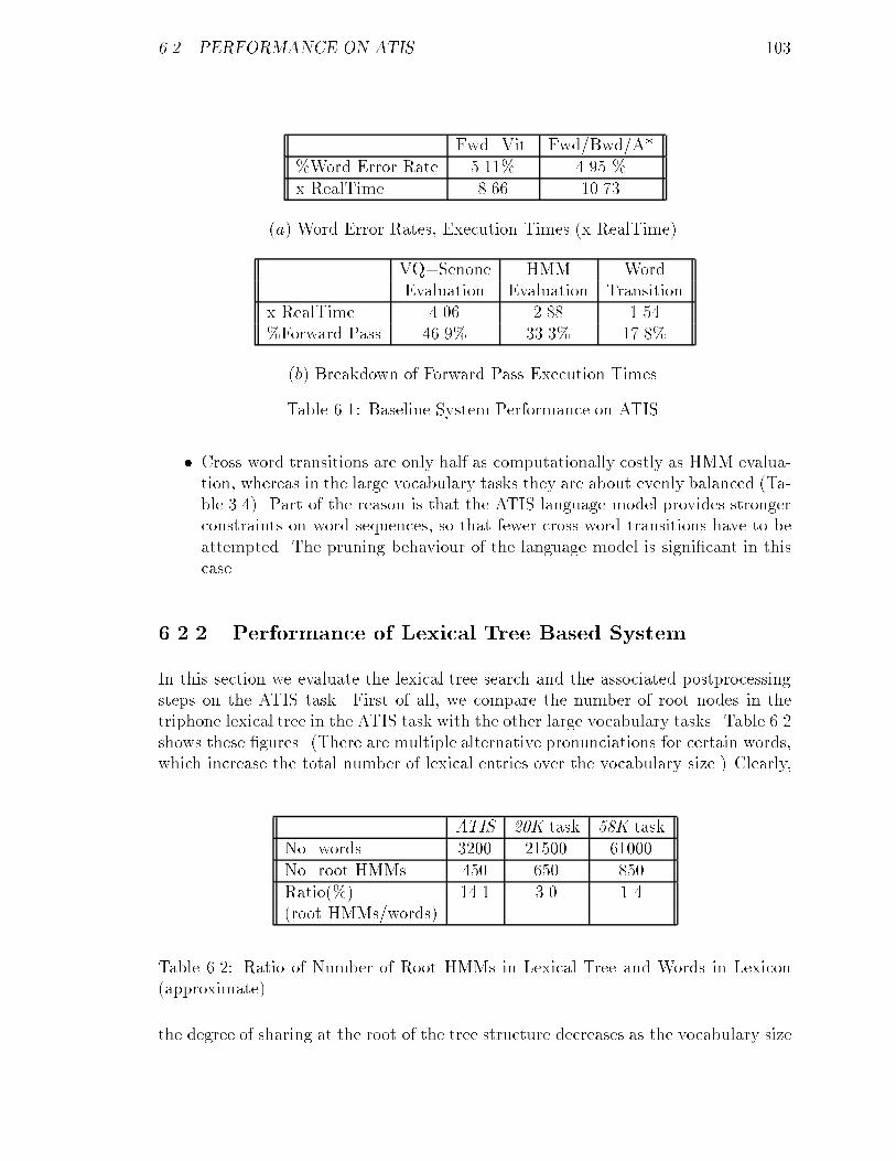
6.2. PERFORMANCE ON ATIS 103
Fwd. Vit. Fwd/Bwd/A*%Word Error Rate 5.11% 4.95 %x RealTime 8.66 10.73
(a) Word Error Rates, Execution Times (x RealTime).
VQ+Senone HMM WordEvaluation Evaluation Transition
x RealTime 4.06 2.88 1.54%Forward Pass 46.9% 33.3% 17.8%
(b) Breakdown of Forward Pass Execution Times.
Table 6.1: Baseline System Performance on ATIS.
� Cross word transitions are only half as computationally costly as HMM evalua-tion, whereas in the large vocabulary tasks they are about evenly balanced (Ta-ble 3.4). Part of the reason is that the ATIS language model provides strongerconstraints on word sequences, so that fewer cross-word transitions have to beattempted. The pruning behaviour of the language model is signi�cant in thiscase.
6.2.2 Performance of Lexical Tree Based System
In this section we evaluate the lexical tree search and the associated postprocessingsteps on the ATIS task. First of all, we compare the number of root nodes in thetriphone lexical tree in the ATIS task with the other large vocabulary tasks. Table 6.2shows these �gures. (There are multiple alternative pronunciations for certain words,which increase the total number of lexical entries over the vocabulary size.) Clearly,
ATIS 20K task 58K taskNo. words 3200 21500 61000No. root HMMs 450 650 850Ratio(%) 14.1 3.0 1.4(root HMMs/words)
Table 6.2: Ratio of Number of Root HMMs in Lexical Tree and Words in Lexicon(approximate).
the degree of sharing at the root of the tree structure decreases as the vocabulary size
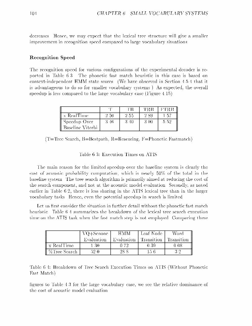
104 CHAPTER 6. SMALL VOCABULARY SYSTEMS
decreases. Hence, we may expect that the lexical tree structure will give a smallerimprovement in recognition speed compared to large vocabulary situations.
Recognition Speed
The recognition speed for various con�gurations of the experimental decoder is re-ported in Table 6.3. The phonetic fast match heuristic in this case is based oncontext-independent HMM state scores. (We have observed in Section 4.5.4 that itis advantageous to do so for smaller vocabulary systems.) As expected, the overallspeedup is less compared to the large vocabulary case (Figure 4.15).
T TB TRB FTRBx RealTime 2.50 2.55 2.89 1.57Speedup Over 3.46 3.40 3.00 5.52Baseline Viterbi
(T=Tree Search, B=Bestpath, R=Rescoring, F=Phonetic Fastmatch)
Table 6.3: Execution Times on ATIS.
The main reason for the limited speedup over the baseline system is clearly thecost of acoustic probability computation, which is nearly 50% of the total in thebaseline system. The tree search algorithm is primarily aimed at reducing the cost ofthe search component, and not at the acoustic model evaluation. Secondly, as notedearlier in Table 6.2, there is less sharing in the ATIS lexical tree than in the largervocabulary tasks. Hence, even the potential speedup in search is limited.
Let us �rst consider the situation in further detail without the phonetic fast matchheuristic. Table 6.4 summarizes the breakdown of the lexical tree search executiontime on the ATIS task when the fast match step is not employed. Comparing these
VQ+Senone HMM Leaf Node WordEvaluation Evaluation Transition Transition
x RealTime 1.30 0.72 0.39 0.08%Tree Search 52.0 28.8 15.6 3.2
Table 6.4: Breakdown of Tree Search Execution Times on ATIS (Without PhoneticFast Match).
�gures to Table 4.3 for the large vocabulary case, we see the relative dominance ofthe cost of acoustic model evaluation.
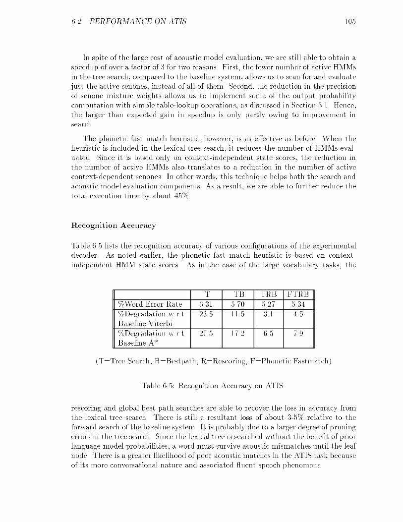
6.2. PERFORMANCE ON ATIS 105
In spite of the large cost of acoustic model evaluation, we are still able to obtain aspeedup of over a factor of 3 for two reasons. First, the fewer number of active HMMsin the tree search, compared to the baseline system, allows us to scan for and evaluatejust the active senones, instead of all of them. Second, the reduction in the precisionof senone mixture weights allows us to implement some of the output probabilitycomputation with simple table-lookup operations, as discussed in Section 5.1. Hence,the larger than expected gain in speedup is only partly owing to improvement insearch.
The phonetic fast match heuristic, however, is as e�ective as before. When theheuristic is included in the lexical tree search, it reduces the number of HMMs eval-uated. Since it is based only on context-independent state scores, the reduction inthe number of active HMMs also translates to a reduction in the number of activecontext-dependent senones. In other words, this technique helps both the search andacoustic model evaluation components. As a result, we are able to further reduce thetotal execution time by about 45%.
Recognition Accuracy
Table 6.5 lists the recognition accuracy of various con�gurations of the experimentaldecoder. As noted earlier, the phonetic fast match heuristic is based on context-independent HMM state scores. As in the case of the large vocabulary tasks, the
T TB TRB FTRB%Word Error Rate 6.31 5.70 5.27 5.34%Degradation w.r.t. 23.5 11.5 3.1 4.5Baseline Viterbi%Degradation w.r.t. 27.5 17.2 6.5 7.9Baseline A*
(T=Tree Search, B=Bestpath, R=Rescoring, F=Phonetic Fastmatch)
Table 6.5: Recognition Accuracy on ATIS.
rescoring and global best path searches are able to recover the loss in accuracy fromthe lexical tree search. There is still a resultant loss of about 3-5% relative to theforward search of the baseline system. It is probably due to a larger degree of pruningerrors in the tree search. Since the lexical tree is searched without the bene�t of priorlanguage model probabilities, a word must survive acoustic mismatches until the leafnode. There is a greater likelihood of poor acoustic matches in the ATIS task becauseof its more conversational nature and associated uent speech phenomena.
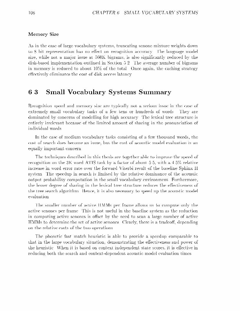
106 CHAPTER 6. SMALL VOCABULARY SYSTEMS
Memory Size
As in the case of large vocabulary systems, truncating senone mixture weights downto 8 bit representation has no e�ect on recognition accuracy. The language modelsize, while not a major issue at 560K bigrams, is also signi�cantly reduced by thedisk-based implementation outlined in Section 5.2. The average number of bigramsin memory is reduced to about 10% of the total. Once again, the caching strategye�ectively eliminates the cost of disk access latency.
6.3 Small Vocabulary Systems Summary
Recognition speed and memory size are typically not a serious issue in the case ofextremely small vocabulary tasks of a few tens or hundreds of words. They aredominated by concerns of modelling for high accuracy. The lexical tree structure isentirely irrelevant because of the limited amount of sharing in the pronunciation ofindividual words.
In the case of medium vocabulary tasks consisting of a few thousand words, thecost of search does become an issue, but the cost of acoustic model evaluation is anequally important concern.
The techniques described in this thesis are together able to improve the speed ofrecognition on the 3K word ATIS task by a factor of about 5.5, with a 4.5% relativeincrease in word error rate over the forward Viterbi result of the baseline Sphinx-IIsystem. The speedup in search is limited by the relative dominance of the acousticoutput probability computation in the small vocabulary environment. Furthermore,the lesser degree of sharing in the lexical tree structure reduces the e�ectiveness ofthe tree search algorithm. Hence, it is also necessary to speed up the acoustic modelevaluation.
The smaller number of active HMMs per frame allows us to compute only theactive senones per frame. This is not useful in the baseline system as the reductionin computing active senones is o�set by the need to scan a large number of activeHMMs to determine the set of active senones. Clearly, there is a tradeo�, dependingon the relative costs of the two operations.
The phonetic fast match heuristic is able to provide a speedup comparable tothat in the large vocabulary situation, demonstrating the e�ectiveness and power ofthe heuristic. When it is based on context-independent state scores, it is e�ective inreducing both the search and context-dependent acoustic model evaluation times.
Chapter 7
Conclusion
This thesis work has focussed on the problems relating to the computational e�ciencyof large vocabulary, continuous speech recognition. The foremost concern addressedin this thesis is that of dealing with the large search space associated with this task.This space is so large that brute force approaches can be several orders of magnitudeslower than real-time. The beam search heuristic is able to narrow down the searchspace dramatically by searching only the most likely states at any time. However,searching even this reduced space requires several tens of times real time on currentcomputers. A reduction in the computational load must come from algorithmic andheuristic improvements.
The second issue addressed in this thesis is e�ciency of memory usage. In partic-ular, the acoustic and language models are the largest contributors to memory sizein modern speech recognition systems.
In order to translate the gains made by research systems in recognition accuracyinto practical use, it is necessary to improve the computational and memory e�ciencyof speech recognition systems. It is relatively easy to improve recognition speedand reduce memory requirements while trading away some accuracy, for example byusing tighter beamwidths for most drastic pruning, and by using simpler or moreconstrained acoustic and language models. But it is much harder to improve boththe recognition speed and reduce main memory requirements while preserving theoriginal accuracy.
The main contributions of this thesis are an 8-fold speedup and a 4-fold reductionin the memory size of the CMU Sphinx-II system. We have used the Sphinx-II systemas a baseline for comparison purposes since it has been extensively used in the yearlyARPA evaluations. It is also one of the premier systems, in terms of recognitionaccuracy, of its kind. On large vocabulary tasks the system requires several tensof times real time and 100-200MB of main memory to perform its function. Theexperiments have been performend on several commonly used benchmark test setsand two di�erent vocabulary sizes of about 20K and 58K words.
107
108 CHAPTER 7. CONCLUSION
We �rst present a brief description of the lessons learnt from this work, followedby a summary of its contributions, concluding with some directions for future workbased on this research.
7.1 Summary of Results
The results in this thesis are based on benchmark tests carried out on theWall StreetJournal and North American Business News development and test sets from the Nov.1993 and Nov. 1994 ARPA evaluations. They consist of read speech in a cleanenvironment using high quality, close-talking microphones, and are widely used inthe ARPA speech community. The experiments are carried out using two di�erentvocabulary sizes, of 20,000 words and 58,000 words, respectively. We now summarizethe main results from this thesis below.
� The lexical tree search algorithm is about 5 times faster than the baselineSphinx-II system. The search component alone, excluding the computation ofacoustic output probabilities of senones, is over 7 times faster than the baselinesystem.
� During the lexical tree search, deferring the computation of language modelprobabilities until the leaves of the lexical reduces the cost of such accesses byabout an order of magnitude, compared to the baseline system. It also leads toan optimization whereby about half of these computations in a given frame canbe eliminated by reusing results from an earlier frame.
� The lattice error rate of the word lattice produced by the lexical tree search isabout 2% (excluding out of vocabulary words), and is highly compact. Thismakes it an ideal input for postprocessing steps using more detailed models andsearch algorithms. The number of entries in the word lattice for a 10sec sentenceis typically about 1000. The word lattice size and error rate are comparable tothat of the baseline system.
� Even though the lexical tree search su�ers an increase in word error rate ofabout 20% relative to the baseline system, the loss can be largely recoveredfrom the word lattice. The best path algorithm presented in this thesis �nds aglobally optimum path through the word lattice and brings the word error ratedown to within 7% relative to the baseline system. The computational cost ofthe best path search is negligible.
� The compact word lattice produced by the tree search can be e�ciently postpro-cessed using detailed acoustic models and/or search algorithms. By applyingthe forward Viterbi search algorithm of the baseline system to the word lat-tice, followed by the best path search, we equal the recognition accuracy of the
7.2. CONTRIBUTIONS 109
baseline system. The overall increase in computation with the addition of thepostprocessing step is about 15%.
� The phonetic fast match heuristic improves recognition speed by identifying alimited set of candidate phones to be activated at each frame. Incorporating thisstep into the lexical tree search leads to a further speedup in overall executiontime by a factor of about 1.8 with less than 2% relative increase in word errorrate.
� It is possible to reduce the precision of representation of the statistical databases,and thus reduce their memory requirement, with no signi�cant e�ect on recog-nition accuracy. Thus, a reduction in the precision of senone weight values from32 bits to 8 bits reduces the acoustic model size from about 40MB to about10MB. This result has also been observed by several other sites such as IBM,BBN and Microsoft.
� The compact representation of senone weights in 8 bits enables the computa-tion of senone output probabilities to be implemented by simple table look upoperations. This speeds up the computation by about a factor of 2.
� A disk-based language model, coupled with a simple software caching scheme toload bigrams and trigrams into memory on demand leads to a reduction in itsmemory requirements by over a factor of 5. The fraction of bigrams resident inmemory is reduced to around 15-25% of the total, and that of trigrams to 2-5%of the total number, on average. The caching scheme is e�ective in neutralizingthe cost of disk access latencies. Since there is no change in data representation,there is no loss of accuracy.
In summary, it is possible to reduce the computation time of the Sphinx-II recog-nizer by nearly an order of magnitude and the memory size requirements by a factorof about 4 for large vocabulary continuous speech recognition, with very little loss ofaccuracy. Appendix B contains a summary of the results of signi�cance tests on thedi�erences between the recognition accuracies of the various systems.
As an additional benchmark result, we note that the techniques described in thisthesis are su�ciently robust that the lexical tree based recognizer was used by CMUduring the Nov. 1995 ARPA evaluations.
7.2 Contributions
One of the main contributions of this thesis is in providing a comprehensive accountof the design of a high-performance speech recognition system in its various aspectsof accuracy, speed, and memory usage. One of the underlying questions concerning
110 CHAPTER 7. CONCLUSION
research systems that focus mainly on accuracy, and require large amounts of com-putational power is whether the approaches taken will ever be of practical use. Thiswork suggests that concerns of accuracy and e�ciency are indeed separable compo-nents of speech recognition technology, and lends validity to the ongoing e�ort inimproving accuracy.
The second major contribution of the thesis is the presentation an overall or-ganization of a speech recognition system for large vocabulary, continuous speechrecognition. We contend that a fast but detailed search, such as that provided bythe lexical tree search described in this thesis, is the key step in obtaining a highlycompact and accurate word lattice. The lattice can be searched using more detailedand sophisticated models and search algorithms e�ciently. The use of multi-passsystems is not new. Most current speech recognition systems are of that nature[41, 65, 5, 15, 19, 38]. Many reports cite the savings to be had by postprocessing aword lattice [65, 38] instead of the entire vocabulary. However, the task of actuallyproducing such lattices e�ciently has been relatively unexplored. This is necessaryfor the practical application of accurate, large vocabulary speech recognition and itis addressed in this thesis.
Technically, the thesis presents several other contributions:
� The design and implementation of search using lexical trees. It analyzes thetechnique of deferring the application of language model probabilities until theleaves of the lexical tree in an e�cient way, and reduces the cost of computingthese probabilities by an order of magnitude. Other tree-based searches [39,43, 65, 66, 40] attempt to overcome the problem by creating bigram copies ofthe search tree. This has three problems: the search space is increased, thecost of language model access is still substantial, and the physical memory sizerequirements also increase. Though the lexical tree search presented in thisthesis su�ers some loss of accuracy, the loss is recovered by postprocessing theword lattice output, which can be done e�ciently since the lattice is highlycompact.
� A best path search for global optimization of word lattices. This techniquesearches the word graph formed from word segmentations and scores producedby an earlier pass. It �nds a globally optimum path through the graph, whichcan be accomplished by any textbook shortest path algorithm. When applied tothe word lattice produced by the lexical tree search, it brings the �nal accuracymuch closer to that of the baseline system, largely overcoming the degradationin accuracy incurred by the lexical tree search. Furthermore, it operates in asmall fraction of real time and its cost is negligible. Word lattice searches havebeen proposed in [65, 39], for example, but they are directed more towards usingthe lattice for driving later search passes with more detailed models.
� Use of HMM state output probabilities as a fast match to produce candidate
7.3. FUTURE WORK ON EFFICIENT SPEECH RECOGNITION 111
list of active phones to be searched. This heuristic has the potential to reducethe active search space substantially, depending on the sharpness of the under-lying acoustic models. We have tried two di�erent approaches for determiningthe set of active phones: based on all HMM states, and based on only thecontext-independent states. The former leads to better phone prediction andmore e�ective search pruning, but incurs a �xed cost of evaluating all HMMstate probabilities. The latter does not have this limitation but is somewhatless accurate in predicting active phones. It is more appropriate for smallervocabularies since senone evaluation does not become a bottleneck.
� Precision of representation of statistical models is largely irrelevant for recogni-tion accuracy. Substantial savings in memory space can be obtained by quantiz-ing, clustering, or truncating probability values into few bits. When probabilityvalues are represented in this compact fashion, it is sometimes possible to imple-ment complex operations on them by means of simple table-lookup operations.The space reduction is not speci�c to the lexical tree search algorithm. It hasbeen implemented in the baseline Sphinx-II system as well, with similar results.
� Use of disk-based language models in reducing memory requirements. Bigramsand trigrams are read into memory on demand, but a simple software cachingpolicy e�ectively hides long disk access latencies. The technique is not speci�cto the lexical tree search algorithm. It has been implemented in the baselineSphinx-II system as well, and has proven to be as e�ective.
7.3 Future Work on E�cient Speech Recognition
The e�ciency of speech recognition is ultimately judged by the end application.Transforming today's laboratory versions of speech recognition systems into practicalapplications requires solutions to many other problems. The resource requirements ofcurrent systems|CPU power and memory|are still beyond the capabilities of com-monly available platforms for medium and large vocabulary applications. Further-more, the notion of \performance" extends beyond accuracy, speed and memory size.These factors include, for example, robustness in the presence of noise, adaptationto varying speaking styles and accents, design issues dealing with human-computerinterfaces that are appropriate for speech-based interaction, speech understanding,etc. We consider how research on the following might be useful in this respect.
Combining Word-Level Fast Match With Lexical Tree Search
The speed of recognition systems could be improved by a combination of a word-level fast match algorithm and a lexical tree search. The former typically reducesthe number of candidate words to be searched by at least an order of magnitude.
112 CHAPTER 7. CONCLUSION
Furthermore, the candidates produced at a given instant are likely to be phoneticallyclosely related, which can be exploited e�ectively by the lexical tree search algorithm.We do not know of any detailed report on a system that takes advantage of the twotogether. It is worthwhile studying this problem further. The results presented inthis thesis provide a baseline for comparison purposes.
Robustness to Noise Using Phone Lattices
Normal speech is often interrupted or overshadowed by noise, and recognition duringsuch periods is highly unreliable. The need for con�dence measures attached to recog-nition results has often been felt. The phone lattices produced by the phonetic fastmatch heuristic described in Section 4.5 could be adapted for this purpose. Duringclean speech, there is a distinct separation between the leading active phones andthe remaining inactive ones. Few phones fall within the beam and they are generallyclosely related or readily confusable. Also there is a good correlation between neigh-bouring frames. In the presence of noise, especially non-speech noise, the number ofactive phones within the beamwidth increases signi�cantly. The reason is that the un-derlying acoustic models are unable to classify the noisy speech with any con�dence.There is a much greater degree of confusability within a frame, and little correlationamong active phones between neighbouring frames. One could use these measures todetect regions where the recognition is potentially unreliable. The advantage of thisapproach is that it is inexpensive to compute.
Postprocessing Word Lattices Using Multiple Language Models
This technique pertains to good user interface design. Several practical applicationsof speech recognition deal with the handling of a number of well-de�ned but distincttasks. For example, in a dictation task text input through speech might be inter-spersed with spoken commands to manipulate the document being edited, such as\scroll-up", \previous paragraph", etc. However, it is cumbersome for the user toconstantly have to indicate to the system the type of command or speech that isforthcoming. It is desirable for the system to make that decision after the fact. Sucha task can be accomplished by searching the word lattice output of the lexical treesearch using multiple language models. The dictation task would use two languagemodels, a general purpose one, and a restricted one for editing commands. Initialspeech recognition is always carried out using the general purpose model. Once asentence is recognized and the word lattice is built, it can be searched again, thistime using the constrained language model. If a path through the word lattice isfound, the sentence can be interpreted as an editing command. The compact natureof the word lattice allows such searches to be carried out rapidly.

7.3. FUTURE WORK ON EFFICIENT SPEECH RECOGNITION 113
Rescoring Word Lattices Using Prosodic Models
Word lattices often contain alternative paths that are phonetically identical. Rescor-ing these using conventional acoustic models, however detailed, is unlikely to resolvethem. However, word or context-dependent prosodic models applied to longer unitssuch as syllables can help discriminate between the alternatives. Once again, the com-pact nature of the lattices enables such postprocessing to be performed e�ciently.
Disk-Based Acoustic Models
With the emergence of continuous HMMs for acoustic modelling, demands on CPUpower and memory capacities increase. The availability of compact lattices that canbe rescored with detailed acoustic models alleviates the CPU power problem. It alsoimplies that fewer HMM states are active at any given instant. Furthermore, oncea state becomes active, it remains active for a few more frames. Thus, it may bepossible to use disk-based acoustic models to reduce their memory requirements aswell. One needs to explore caching mechanisms and their e�ectiveness in overcomingdisk access latencies for this purpose.
Design of Scalable Systems
It is important to consider the problem of designing a speech application on a speci�cplatform with given resource constraints. The main criteria are that the applicationshould perform in real time within the CPU and memory capacities of the system.Therefore, it is generally necessary to make trade-o�s regarding the level of sophisti-cation of modelling and search that may be employed. The memory size problem canbe attacked by using less detailed models during the initial search to create a wordlattice, as well as using disk-based mechanisms. The cost of search can be reducedby increasing the degree of sharing in the lexical tree, for example, by using diphoneor even monophone models instead of triphones. The word lattice output may haveto be larger in order to provide an acceptably low lattice error rate, and hence thepostprocessing costs also increase. It is worth investigating the tradeo�s that arepossible in this respect.

114 CHAPTER 7. CONCLUSION
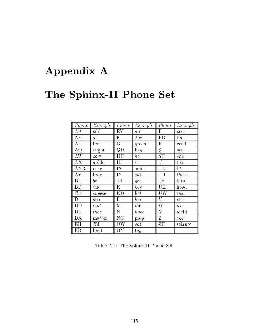
Appendix A
The Sphinx-II Phone Set
Phone Example Phone Example Phone Example
AA odd EY ate P peeAE at F fee PD lipAH hut G green R readAO ought GD bag S seaAW cow HH he SH sheAX abide IH it T teaAXR user IX acid TD litAY hide IY eat TH thetaB be JH gee TS bitsBD dub K key UH hoodCH cheese KD lick UW twoD dee L lee V veeDD dud M me W weDH thee N knee Y yieldDX matter NG ping Z zeeEH Ed OW oat ZH seizureER hurt OY toy
Table A.1: The Sphinx-II Phone Set.
115
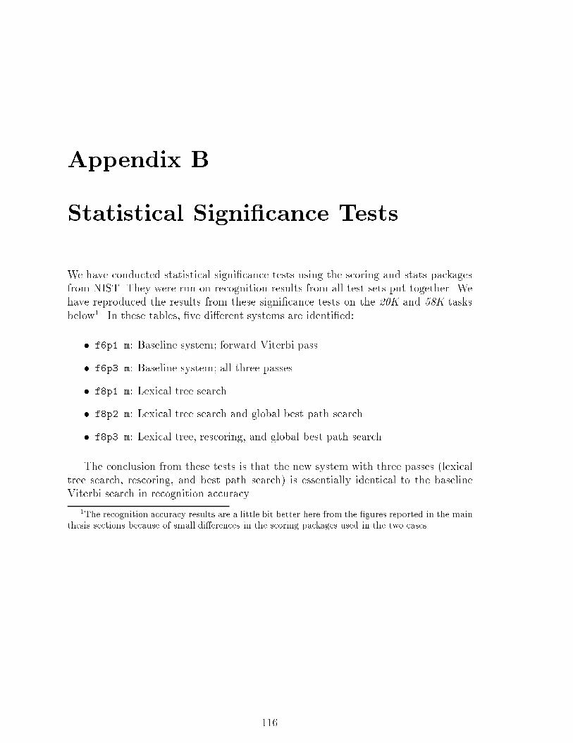
Appendix B
Statistical Signi�cance Tests
We have conducted statistical signi�cance tests using the scoring and stats packagesfrom NIST. They were run on recognition results from all test sets put together. Wehave reproduced the results from these signi�cance tests on the 20K and 58K tasksbelow1. In these tables, �ve di�erent systems are identi�ed:
� f6p1.m: Baseline system; forward Viterbi pass.
� f6p3.m: Baseline system; all three passes.
� f8p1.m: Lexical tree search.
� f8p2.m: Lexical tree search and global best path search.
� f8p3.m: Lexical tree, rescoring, and global best path search.
The conclusion from these tests is that the new system with three passes (lexicaltree search, rescoring, and best path search) is essentially identical to the baselineViterbi search in recognition accuracy.
1The recognition accuracy results are a little bit better here from the �gures reported in the mainthesis sections because of small di�erences in the scoring packages used in the two cases.
116
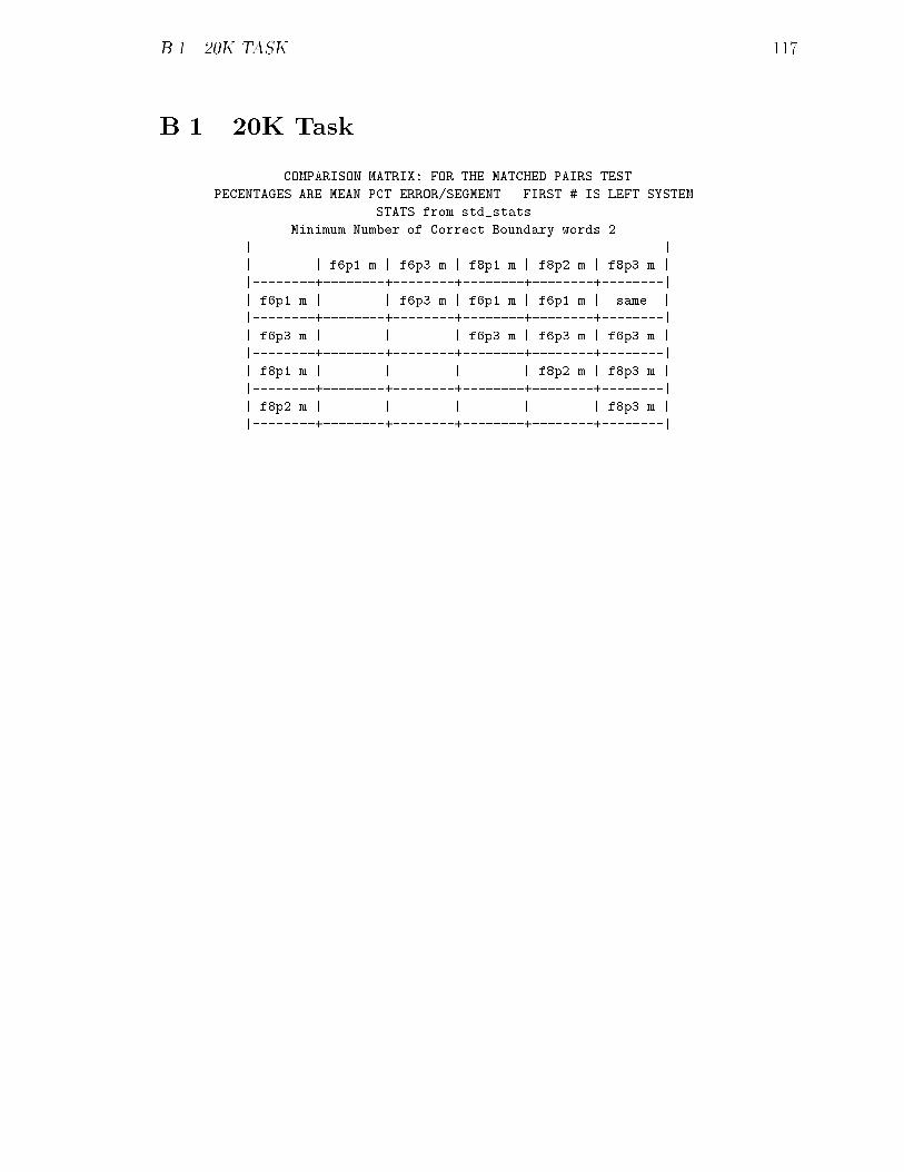
B.1. 20K TASK 117
B.1 20K Task
COMPARISON MATRIX: FOR THE MATCHED PAIRS TEST
PECENTAGES ARE MEAN PCT ERROR/SEGMENT. FIRST # IS LEFT SYSTEM
STATS from std_stats
Minimum Number of Correct Boundary words 2
|-----------------------------------------------------|
| | f6p1.m | f6p3.m | f8p1.m | f8p2.m | f8p3.m |
|--------+--------+--------+--------+--------+--------|
| f6p1.m | | f6p3.m | f6p1.m | f6p1.m | same |
|--------+--------+--------+--------+--------+--------|
| f6p3.m | | | f6p3.m | f6p3.m | f6p3.m |
|--------+--------+--------+--------+--------+--------|
| f8p1.m | | | | f8p2.m | f8p3.m |
|--------+--------+--------+--------+--------+--------|
| f8p2.m | | | | | f8p3.m |
|--------+--------+--------+--------+--------+--------|
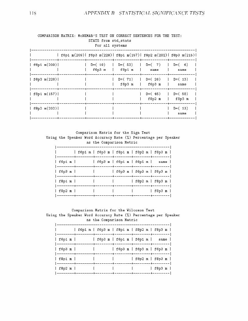
118 APPENDIX B. STATISTICAL SIGNIFICANCE TESTS
COMPARISON MATRIX: McNEMAR'S TEST ON CORRECT SENTENCES FOR THE TEST:
STATS from std_stats
For all systems
|-----------------------------------------------------------------------------|
| | f6p1.m(209)| f6p3.m(228)| f8p1.m(157)| f8p2.m(202)| f8p3.m(215)|
|------------+------------+------------+------------+------------+------------|
| f6p1.m(209)| | D=( 19) | D=( 52) | D=( 7) | D=( 6) |
| | | f6p3.m | f6p1.m | same | same |
|------------+------------+------------+------------+------------+------------|
| f6p3.m(228)| | | D=( 71) | D=( 26) | D=( 13) |
| | | | f6p3.m | f6p3.m | same |
|------------+------------+------------+------------+------------+------------|
| f8p1.m(157)| | | | D=( 45) | D=( 58) |
| | | | | f8p2.m | f8p3.m |
|------------+------------+------------+------------+------------+------------|
| f8p2.m(202)| | | | | D=( 13) |
| | | | | | same |
|------------+------------+------------+------------+------------+------------|
Comparison Matrix for the Sign Test
Using the Speaker Word Accuracy Rate (%) Percentage per Speaker
as the Comparison Metric
|-----------------------------------------------------|
| | f6p1.m | f6p3.m | f8p1.m | f8p2.m | f8p3.m |
|--------+--------+--------+--------+--------+--------|
| f6p1.m | | f6p3.m | f6p1.m | f6p1.m | same |
|--------+--------+--------+--------+--------+--------|
| f6p3.m | | | f6p3.m | f6p3.m | f6p3.m |
|--------+--------+--------+--------+--------+--------|
| f8p1.m | | | | f8p2.m | f8p3.m |
|--------+--------+--------+--------+--------+--------|
| f8p2.m | | | | | f8p3.m |
|--------+--------+--------+--------+--------+--------|
Comparison Matrix for the Wilcoxon Test
Using the Speaker Word Accuracy Rate (%) Percentage per Speaker
as the Comparison Metric
|-----------------------------------------------------|
| | f6p1.m | f6p3.m | f8p1.m | f8p2.m | f8p3.m |
|--------+--------+--------+--------+--------+--------|
| f6p1.m | | f6p3.m | f6p1.m | f6p1.m | same |
|--------+--------+--------+--------+--------+--------|
| f6p3.m | | | f6p3.m | f6p3.m | f6p3.m |
|--------+--------+--------+--------+--------+--------|
| f8p1.m | | | | f8p2.m | f8p3.m |
|--------+--------+--------+--------+--------+--------|
| f8p2.m | | | | | f8p3.m |
|--------+--------+--------+--------+--------+--------|
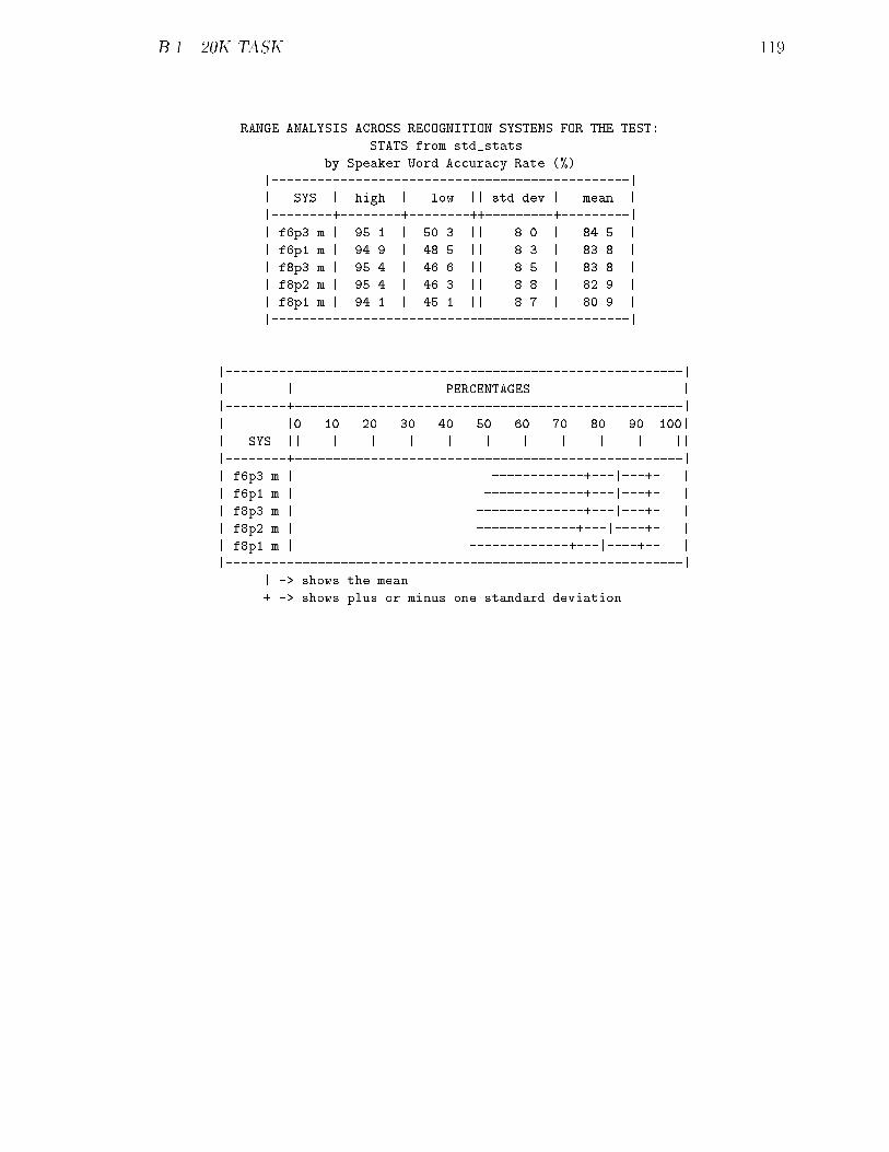
B.1. 20K TASK 119
RANGE ANALYSIS ACROSS RECOGNITION SYSTEMS FOR THE TEST:
STATS from std_stats
by Speaker Word Accuracy Rate (%)
|-----------------------------------------------|
| SYS | high | low || std dev | mean |
|--------+--------+--------++---------+---------|
| f6p3.m | 95.1 | 50.3 || 8.0 | 84.5 |
| f6p1.m | 94.9 | 48.5 || 8.3 | 83.8 |
| f8p3.m | 95.4 | 46.6 || 8.5 | 83.8 |
| f8p2.m | 95.4 | 46.3 || 8.8 | 82.9 |
| f8p1.m | 94.1 | 45.1 || 8.7 | 80.9 |
|-----------------------------------------------|
|------------------------------------------------------------|
| | PERCENTAGES |
|--------+---------------------------------------------------|
| |0 10 20 30 40 50 60 70 80 90 100|
| SYS || | | | | | | | | | ||
|--------+---------------------------------------------------|
| f6p3.m | ------------+---|---+- |
| f6p1.m | -------------+---|---+- |
| f8p3.m | --------------+---|---+- |
| f8p2.m | -------------+---|----+- |
| f8p1.m | -------------+---|----+-- |
|------------------------------------------------------------|
| -> shows the mean
+ -> shows plus or minus one standard deviation
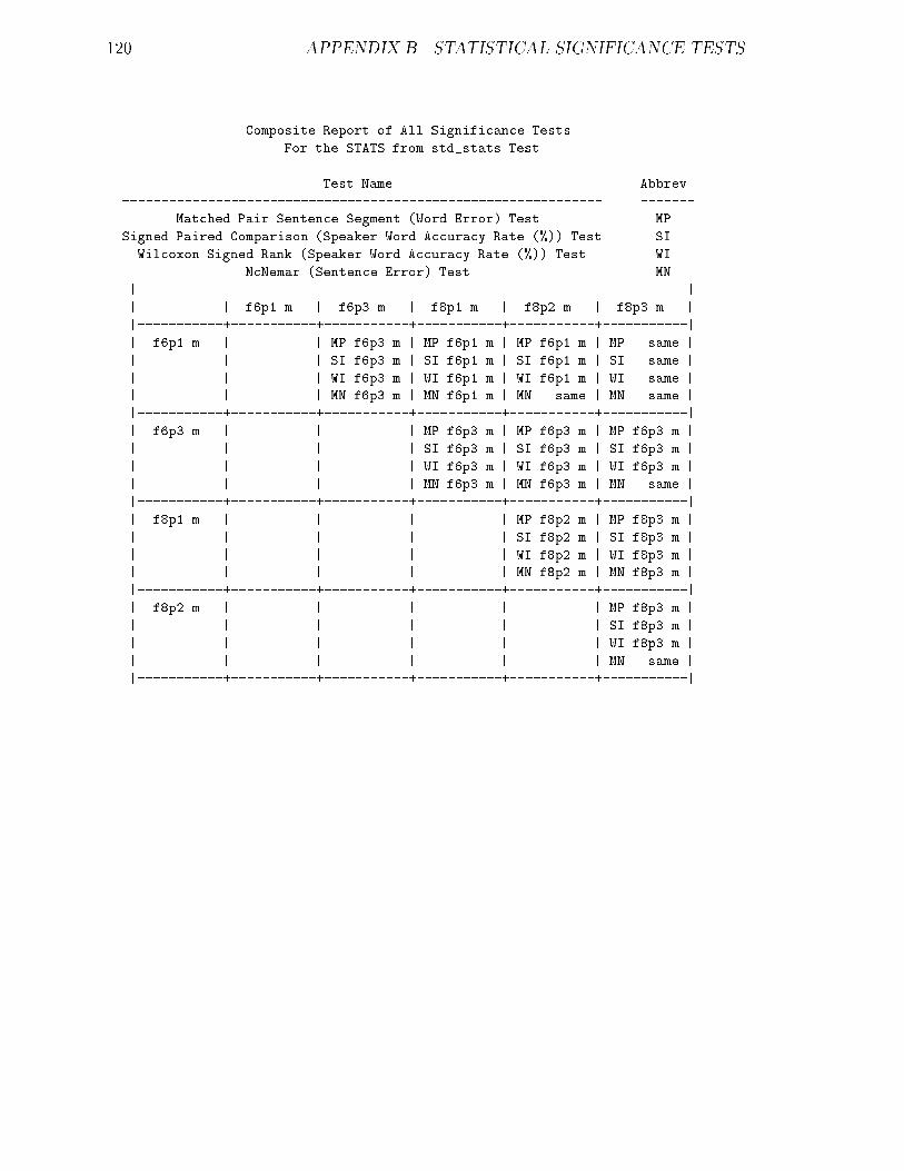
120 APPENDIX B. STATISTICAL SIGNIFICANCE TESTS
Composite Report of All Significance Tests
For the STATS from std_stats Test
Test Name Abbrev.
-------------------------------------------------------------- -------
Matched Pair Sentence Segment (Word Error) Test MP
Signed Paired Comparison (Speaker Word Accuracy Rate (%)) Test SI
Wilcoxon Signed Rank (Speaker Word Accuracy Rate (%)) Test WI
McNemar (Sentence Error) Test MN
|-----------------------------------------------------------------------|
| | f6p1.m | f6p3.m | f8p1.m | f8p2.m | f8p3.m |
|-----------+-----------+-----------+-----------+-----------+-----------|
| f6p1.m | | MP f6p3.m | MP f6p1.m | MP f6p1.m | MP same |
| | | SI f6p3.m | SI f6p1.m | SI f6p1.m | SI same |
| | | WI f6p3.m | WI f6p1.m | WI f6p1.m | WI same |
| | | MN f6p3.m | MN f6p1.m | MN same | MN same |
|-----------+-----------+-----------+-----------+-----------+-----------|
| f6p3.m | | | MP f6p3.m | MP f6p3.m | MP f6p3.m |
| | | | SI f6p3.m | SI f6p3.m | SI f6p3.m |
| | | | WI f6p3.m | WI f6p3.m | WI f6p3.m |
| | | | MN f6p3.m | MN f6p3.m | MN same |
|-----------+-----------+-----------+-----------+-----------+-----------|
| f8p1.m | | | | MP f8p2.m | MP f8p3.m |
| | | | | SI f8p2.m | SI f8p3.m |
| | | | | WI f8p2.m | WI f8p3.m |
| | | | | MN f8p2.m | MN f8p3.m |
|-----------+-----------+-----------+-----------+-----------+-----------|
| f8p2.m | | | | | MP f8p3.m |
| | | | | | SI f8p3.m |
| | | | | | WI f8p3.m |
| | | | | | MN same |
|-----------+-----------+-----------+-----------+-----------+-----------|
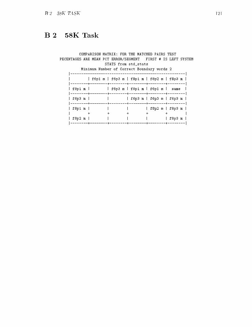
B.2. 58K TASK 121
B.2 58K Task
COMPARISON MATRIX: FOR THE MATCHED PAIRS TEST
PECENTAGES ARE MEAN PCT ERROR/SEGMENT. FIRST # IS LEFT SYSTEM
STATS from std_stats
Minimum Number of Correct Boundary words 2
|-----------------------------------------------------|
| | f6p1.m | f6p3.m | f8p1.m | f8p2.m | f8p3.m |
|--------+--------+--------+--------+--------+--------|
| f6p1.m | | f6p3.m | f6p1.m | f6p1.m | same |
|--------+--------+--------+--------+--------+--------|
| f6p3.m | | | f6p3.m | f6p3.m | f6p3.m |
|--------+--------+--------+--------+--------+--------|
| f8p1.m | | | | f8p2.m | f8p3.m |
|--------+--------+--------+--------+--------+--------|
| f8p2.m | | | | | f8p3.m |
|--------+--------+--------+--------+--------+--------|
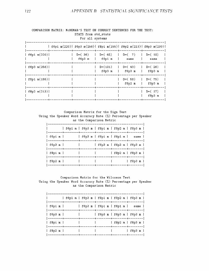
122 APPENDIX B. STATISTICAL SIGNIFICANCE TESTS
COMPARISON MATRIX: McNEMAR'S TEST ON CORRECT SENTENCES FOR THE TEST:
STATS from std_stats
For all systems
|-----------------------------------------------------------------------------|
| | f6p1.m(220)| f6p3.m(256)| f8p1.m(155)| f8p2.m(213)| f8p3.m(230)|
|------------+------------+------------+------------+------------+------------|
| f6p1.m(220)| | D=( 36) | D=( 65) | D=( 7) | D=( 10) |
| | | f6p3.m | f6p1.m | same | same |
|------------+------------+------------+------------+------------+------------|
| f6p3.m(256)| | | D=(101) | D=( 43) | D=( 26) |
| | | | f6p3.m | f6p3.m | f6p3.m |
|------------+------------+------------+------------+------------+------------|
| f8p1.m(155)| | | | D=( 58) | D=( 75) |
| | | | | f8p2.m | f8p3.m |
|------------+------------+------------+------------+------------+------------|
| f8p2.m(213)| | | | | D=( 17) |
| | | | | | f8p3.m |
|------------+------------+------------+------------+------------+------------|
Comparison Matrix for the Sign Test
Using the Speaker Word Accuracy Rate (%) Percentage per Speaker
as the Comparison Metric
|-----------------------------------------------------|
| | f6p1.m | f6p3.m | f8p1.m | f8p2.m | f8p3.m |
|--------+--------+--------+--------+--------+--------|
| f6p1.m | | f6p3.m | f6p1.m | f6p1.m | same |
|--------+--------+--------+--------+--------+--------|
| f6p3.m | | | f6p3.m | f6p3.m | f6p3.m |
|--------+--------+--------+--------+--------+--------|
| f8p1.m | | | | f8p2.m | f8p3.m |
|--------+--------+--------+--------+--------+--------|
| f8p2.m | | | | | f8p3.m |
|--------+--------+--------+--------+--------+--------|
Comparison Matrix for the Wilcoxon Test
Using the Speaker Word Accuracy Rate (%) Percentage per Speaker
as the Comparison Metric
|-----------------------------------------------------|
| | f6p1.m | f6p3.m | f8p1.m | f8p2.m | f8p3.m |
|--------+--------+--------+--------+--------+--------|
| f6p1.m | | f6p3.m | f6p1.m | f6p1.m | same |
|--------+--------+--------+--------+--------+--------|
| f6p3.m | | | f6p3.m | f6p3.m | f6p3.m |
|--------+--------+--------+--------+--------+--------|
| f8p1.m | | | | f8p2.m | f8p3.m |
|--------+--------+--------+--------+--------+--------|
| f8p2.m | | | | | f8p3.m |
|--------+--------+--------+--------+--------+--------|
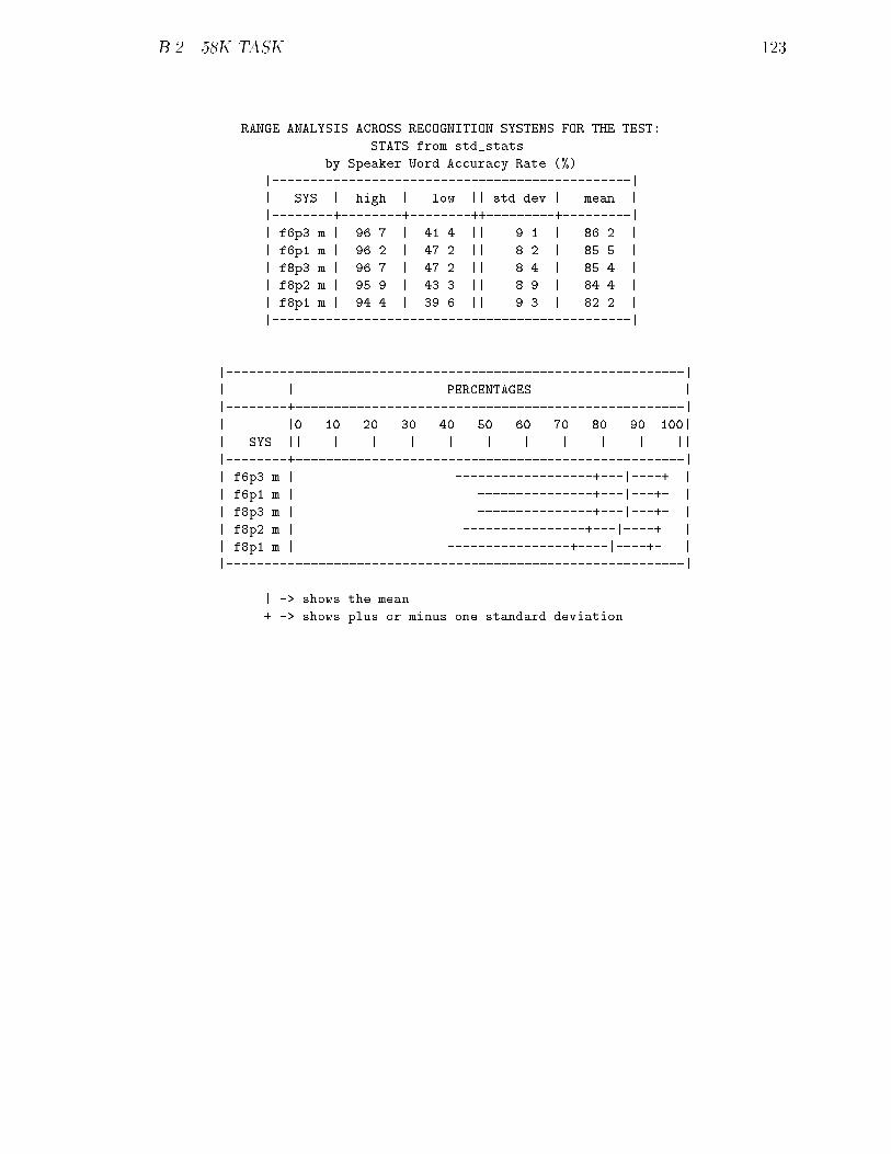
B.2. 58K TASK 123
RANGE ANALYSIS ACROSS RECOGNITION SYSTEMS FOR THE TEST:
STATS from std_stats
by Speaker Word Accuracy Rate (%)
|-----------------------------------------------|
| SYS | high | low || std dev | mean |
|--------+--------+--------++---------+---------|
| f6p3.m | 96.7 | 41.4 || 9.1 | 86.2 |
| f6p1.m | 96.2 | 47.2 || 8.2 | 85.5 |
| f8p3.m | 96.7 | 47.2 || 8.4 | 85.4 |
| f8p2.m | 95.9 | 43.3 || 8.9 | 84.4 |
| f8p1.m | 94.4 | 39.6 || 9.3 | 82.2 |
|-----------------------------------------------|
|------------------------------------------------------------|
| | PERCENTAGES |
|--------+---------------------------------------------------|
| |0 10 20 30 40 50 60 70 80 90 100|
| SYS || | | | | | | | | | ||
|--------+---------------------------------------------------|
| f6p3.m | ------------------+---|----+ |
| f6p1.m | ---------------+---|---+- |
| f8p3.m | ---------------+---|---+- |
| f8p2.m | ----------------+---|----+ |
| f8p1.m | ----------------+----|----+- |
|------------------------------------------------------------|
| -> shows the mean
+ -> shows plus or minus one standard deviation
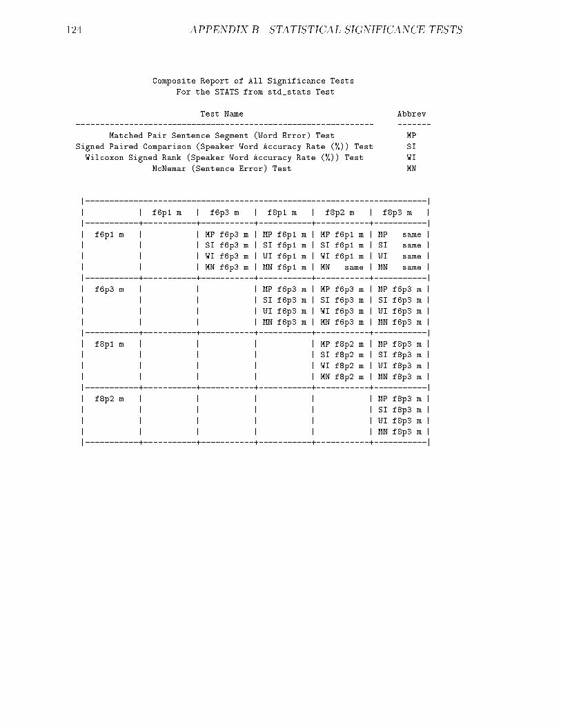
124 APPENDIX B. STATISTICAL SIGNIFICANCE TESTS
Composite Report of All Significance Tests
For the STATS from std_stats Test
Test Name Abbrev.
-------------------------------------------------------------- -------
Matched Pair Sentence Segment (Word Error) Test MP
Signed Paired Comparison (Speaker Word Accuracy Rate (%)) Test SI
Wilcoxon Signed Rank (Speaker Word Accuracy Rate (%)) Test WI
McNemar (Sentence Error) Test MN
|-----------------------------------------------------------------------|
| | f6p1.m | f6p3.m | f8p1.m | f8p2.m | f8p3.m |
|-----------+-----------+-----------+-----------+-----------+-----------|
| f6p1.m | | MP f6p3.m | MP f6p1.m | MP f6p1.m | MP same |
| | | SI f6p3.m | SI f6p1.m | SI f6p1.m | SI same |
| | | WI f6p3.m | WI f6p1.m | WI f6p1.m | WI same |
| | | MN f6p3.m | MN f6p1.m | MN same | MN same |
|-----------+-----------+-----------+-----------+-----------+-----------|
| f6p3.m | | | MP f6p3.m | MP f6p3.m | MP f6p3.m |
| | | | SI f6p3.m | SI f6p3.m | SI f6p3.m |
| | | | WI f6p3.m | WI f6p3.m | WI f6p3.m |
| | | | MN f6p3.m | MN f6p3.m | MN f6p3.m |
|-----------+-----------+-----------+-----------+-----------+-----------|
| f8p1.m | | | | MP f8p2.m | MP f8p3.m |
| | | | | SI f8p2.m | SI f8p3.m |
| | | | | WI f8p2.m | WI f8p3.m |
| | | | | MN f8p2.m | MN f8p3.m |
|-----------+-----------+-----------+-----------+-----------+-----------|
| f8p2.m | | | | | MP f8p3.m |
| | | | | | SI f8p3.m |
| | | | | | WI f8p3.m |
| | | | | | MN f8p3.m |
|-----------+-----------+-----------+-----------+-----------+-----------|

Bibliography
[1] Alleva, F., Hon, H., Hwang, M., Rosenfeld, R. and Weide, R. ApplyingSPHINX-II to the DARPA Wall Street Journal CSR Task. In Proceed-ings of Speech and Natural Language Workshop, Feb. 1992, pp393-398.
[2] Alleva, F., Huang, X., and Hwang, M. An Improved Search Algorithm forContinuous Speech Recognition. In IEEE International Conference on
Acoustics, Speech, and Signal Processing, 1993.
[3] Antoniol, G., Brugnara, F., Cettolo, M. and Federico, M. Language ModelRepresentation for Beam-Search Decoding. In IEEE International Con-
ference on Acoustics, Speech, and Signal Processing, May 1995, pp588-591.
[4] Bahl, L.R., Bakis, R., Cohen, P.S., Cole, A.G., Jelinek, F., Lewis, B.L. andMercer, R.L. Further Results on the Recognition of a Continuously ReadNatural Corpus. In IEEE International Conference on Acoustics,
Speech, and Signal Processing, Apr. 1980, pp 872-876.
[5] Bahl, L.R., Balakrishnan-Aiyer, S., Franz, M., Gopalakrishnan, P.S.,Gopinath, R., Novak, M., Padmanabhan, M. and Roukos, S. The IBMLarge Vocabulary Continuous Speech Recognition System for the ARPANAB News Task. In Proceedings of ARPA Spoken Language Sys-
tem Technology Workshop, Jan. 1995, pp 121-126.
[6] Bahl, L.R., Brown, P.F., DeSouza, P.V. and Mercer, R.L. Obtaining CandidateWords by Polling in a Large Vocabulary Speech Recognition System. InIEEE International Conference on Acoustics, Speech, and Signal
Processing, 1988.
[7] Bahl, L.R., De Gennaro, V., Gopalakrishnan, P.S. and Mercer, R.L.A Fast Ap-proximate Acoustic Match for Large Vocabulary Speech Recognition. IEEETransactions on Speech and Audio Processing, Vol. 1, No. 1, Jan1993, pp 59-67.
125
126 Bibliography
[8] Bahl, L.R., DeSouza, P.V., Gopalakrishnan, P.S., Nahamoo, D. and Pich-eney, M.A Fast Match for Continuous Speech Recognition Using AllophonicModels. In IEEE International Conference on Acoustics, Speech,
and Signal Processing, 1992, vol.I, pp. I-17 { I-21.
[9] Bahl, L.R., Jelinek, F. and Mercer, R. A Maximum Likelihood Approachto Continuous Speech Recognition. In IEEE Transactions on Pattern
Analysis and Machine Intelligence, Vol. PAMI-5, No. 2, Mar. 1983,pp. 179-190.
[10] Baker, J.K. The DRAGON System{An Overview. In IEEE Transactions on
Acoustics, Speech, and Signal Processing, ASSP-23(1), Feb. 1975,pp. 24-29.
[11] Baum, L.E. An Inequality and Associated Maximization Technique in Statis-tical Estimation of Probabilistic Functions of Markov Processes. Inequal-ities 3:1-8, 1972.
[12] Bellegarda, J. and Nahamoo, D. Tied Mixture Continuous Parameter Modelingfor Speech Recognition. In IEEE Transactions on Acoustics, Speech,
and Signal Processing, Dec. 1990, pp 2033-2045.
[13] Bisiani, R. and Ravishankar, M PLUS: A Distributed Shared-Memory System.17th International Symposium on Computer Architecture, May 1990, pp.115-124.
[14] Bisiani, R. and Ravishankar, M Design and Implementation of the PLUS Mul-tiprocessor Internal report, School of Computer Science, Carnegie MellonUniversity, Pittsburgh, Jan. 1991.
[15] Chase, L., Rosenfeld, R., Hauptmann, A., Ravishankar, M., Thayer, E., Place-way, P., Weide, R. and Lu, C. Improvements in Language, Lexical, andPhonetic Modeling in Sphinx-II. InProceedings of ARPA Spoken Lan-
guage Systems Technology Workshop, Jan. 1995, pp. 60-65.
[16] Cooper, E.C. and Draves, R.P. C Threads. Technical Report, School of Com-puter Science, Carnegie Mellon University, Nov. 1990.
[17] Coremen, T.H., Leiserson, C.E. and Rivest, R.L. Introduction to Algo-
rithms, The MIT Press, Cambridge, Massachusetts, 1992.
[18] Gauvain, J.L., Lamel, L.F., Adda, G., and Adda-Decker, M. The LIMSI Nov93WSJ System. In Proceedings of ARPA Speech and Natural Lan-
guage Workshop, Mar. 1994, pp 125-128.
Bibliography 127
[19] Gauvain, J.L., Lamel, L. and Adda-Decker, M. Developments in Large Vo-cabulary Dictation: The LIMSI Nov94 NAB System. In Proceedings
of ARPA Spoken Language Systems Technology Workshop, Jan.1995, pp. 131-138.
[20] Gillick, L.S. and Roth, R. A Rapid Match Algorithm for Continuous SpeechRecognition. In Proceedings of DARPA Speech and Natural Lan-
guage Workshop, Jun. 1990, pp. 170-172.
[21] Gopalakrishnan, P.S., Bahl, L.R., and Mercer, R.L. A Tree Search Strategyfor Large-Vocabulary Continuous Speech Recognition. In IEEE Interna-
tional Conference on Acoustics, Speech, and Signal Processing,May 1995, pp 572-575.
[22] Gopalakrishnan, P.S., Nahamoo, D., Padmanabhan, M. and Picheny, M.A. AChannel-Bank-Based Phone Detection Strategy. In IEEE International
Conference on Acoustics, Speech, and Signal Processing, April1994, Vol II, pp 161-164.
[23] Gopinath, R. et al. The IBM continuous speech recognition system on demon-stration. ARPA Spoken Language Systems Technology Workshop,Jan. 1995.
[24] Hauptmann, A. et al. The News-on-Demand demonstration. In ARPA
Speech Recognition Workshop, Feb. 1996.
[25] Huang, X., Acero, A., Alleva, F., Beeferman, D., Hwang, M. and Mahajan,M. From CMU Sphinx-II to Microsoft Whisper{Making Speech RecognitionUsable. In Automatic Speech and Speaker Recognition{Advanced
Topics, Lee, Paliwal, and Soong, editors, Kluwer Publishers, 1994.
[26] Huang, X., Acero, A., Alleva, F., Hwang, M., Jiang, L. and Mahajan, M. Mi-crosoft Windows Highly Intelligent Speech Recognizer: Whisper. In IEEEInternational Conference on Acoustics, Speech, and Signal Pro-
cessing, May 1995, Vol. 1, pp. 93-96.
[27] Hwang, Mei-Yuh. Subphonetic Acoustic Modeling for Speaker-IndependentContinuous Speech Recognition. Ph.D. thesis, Tech Report No. CMU-CS-93-230, Computer Science Department, Carnegie Mellon University, Dec.1993.
[28] Hwang, M. and Huang X. Shared-Distribution Hidden Markov Models forSpeech Recognition. In IEEE Transactions on Speech and Audio Pro-
cessing, Oct. 1993, pp 414-420.
128 Bibliography
[29] Jelinek, F. Continuous Speech Recognition by Statistical Methods. InProceed-ings of the IEEE, Vol. 64, No. 4, Apr. 1976, pp. 532-556.
[30] Katz, S.M. Estimation of Probabilities from Sparse Data for the LanguageModel Component of a Speech Recognizer. In IEEE Transactions on
Acoustics, Speech and Signal Processing, vol. ASSP-35, Mar. 87, pp.400-401.
[31] Kershaw, D.J., Robinson, A.J., and Renals, S.J. The 1995 ABBOT Hy-brid Connectionist-HMM Large-Vocabulary Recognition System. In ARPASpeech Recognition Workshop, Feb. 1996.
[32] Lee, K. Large Vocabulary Speaker-Independent Continuous Speech Recogni-tion: The SPHINX System. Ph.D. thesis, Computer Science Department,Carnegie Mellon University, April 1988.
[33] Lee, K. Context-Dependent Phonetic Hidden Markov Models for ContinuousSpeech Recognition. In IEEE Transactions on Acoustics, Speech, and
Signal Processing, Apr. 1990, pp 599-609.
[34] Lee, K. Context-Dependent Phonetic Hidden Markov Models for Speaker-Independent Continuous Speech Recognition. In Readings in Speech
Recognition, ed. Waibel, A. and Lee, K. Morgan Kaufmann Publishers,San Mateo, CA, 1990, pp. 347-365.
[35] Lee, K., Hon, H., and Reddy, R. An Overview of the SPHINX Speech Recogni-tion System. In IEEE Transactions on Acoustics, Speech, and Signal
Processing, Jan 1990, pp 35-45.
[36] Ljolje, A., Riley, M., Hindle, D. and Pereira, F. The AT&T 60,000 WordSpeech-To-Text System. In Proceedings of ARPA Spoken Language
System Technology Workshop, Jan. 1995, pp. 162-165.
[37] Lowerre, B. The Harpy Speech Understanding System. Ph.D. thesis, ComputerScience Department, Carnegie Mellon University, Apr 1976.
[38] Murveit, H., Butzberger, J., Digalakis, V. and Weintraub, M. Large-Vocabulary Dictation Using SRI's Decipher Speech Recognition System:Progressive Search Techniques. In IEEE International Conference on
Acoustics, Speech, and Signal Processing, Apr. 1993, vol.II, pp. II-319 { II-322.
[39] Murveit, H., Monaco, P., Digalakis, V. and Butzberger, J. Techniques toAchieve an Accurate Real-Time Large-Vocabulary Speech Recognition Sys-tem. InProceedings of ARPA Human Language Technology Work-
shop, Mar. 1994, pp 368-373.
Bibliography 129
[40] Ney, H., Haeb-Umbach, R. and Tran, B.-H. Improvements in Beam Searchfor 10000-Word Continuous Speech Recognition. In IEEE International
Conference on Acoustics, Speech, and Signal Processing, Mar.1992, vol.I, pp. I-9 { I-12.
[41] Nguyen, L., Anastasakos, T., Kubala, F., LaPre, C., Makhoul, J., Schwartz,R., Yuan, N., Zavaliagkos, G. and Zhao, Y. The 1994 BBN/BYBLOSSpeech Recognition System. In Proceedings of ARPA Spoken Lan-
guage Systems Technology Workshop, Jan. 1995, pp. 77-81.
[42] Nilsson, N.J. Problem Solving Methods in Arti�cial Intelligence. McGraw-Hill,New York, 1971.
[43] Normandin, Y., Bowness, D., Cardin, R., Drouin, C., Lacouture, R. andLazarides, A. CRIM's November 94 Continuous Speech Recognition Sys-tem. In Proceedings of ARPA Speech and Natural Language
Workshop, Jan. 1995, pp 153-155.
[44] Odell, J.J., Valtchev, V., Woodland, P.C. and Young, S.J. A One Pass De-coder Design for Large Vocabulary Recognition. InProceedings of ARPAHuman Language Technology Workshop, Princeton, 1994.
[45] Pallett, D.S., Fiscus, J.G., Fisher, W.M., Garofolo, J.S., Lund, B.A., andPrzybocki, M.A. 1993 Benchmark Tests for the ARPA Spoken LanguageProgram. In Proceedings of ARPA Speech and Natural Language
Workshop, Mar. 1994, pp 15-40.
[46] Pallett, D.S., Fiscus, J.G., Fisher, W.M., Garofolo, J.S., Lund, B.A., Martin,A. and Przybocki, M.A. 1994 Benchmark Tests for the ARPA Spoken Lan-guage Program. In Proceedings of ARPA Spoken Language Systems
Technology Workshop, Jan. 1995, pp 5-38.
[47] Pallett, D.S., Fiscus, J.G., Fisher, W.M., Garofolo, J.S., Martin, A. and Przy-bocki, M.A. 1995 HUB-3 NIST Multiple Microphone Corpus BenchmarkTests. In ARPA Speech Recognition Workshop, Feb. 1996.
[48] Pallett, D.S., Fiscus, J.G., Garofolo, J.S., and Przybocki, M.A. 1995 Hub-4 \Dry Run" Broadcast Materials Benchmark Tests. In ARPA Speech
Recognition Workshop, Feb. 1996.
[49] Patel, S. A Lower-Complexity Viterbi Algorithm. In IEEE International
Conference on Acoustics, Speech, and Signal Processing, May1995, Vol. 1, pp. 592-595.
130 Bibliography
[50] Paul, Douglas B. An E�cient A* Stack Decoder Algorithm for ContinuousSpeech Recognition with a Stochastic Language Model. In Proceedings ofDARPA Speech and Natural Language Workshop, Feb. 1992, pp405-409.
[51] Price, P., Fisher, W.M., Bernstein, J. and Pallet, D.S. The DARPA 1000-Word Resource Management Database for Continuous Speech Recognition.In IEEE International Conference on Acoustics, Speech, and Sig-
nal Processing, 1988.
[52] Rabiner, L.R. A Tutorial on Hidden Markov Models and Selected Applicationsin Speech Recognition. In Readings in Speech Recognition, ed.Waibel,A. and Lee, K. Morgan Kaufmann Publishers, San Mateo, CA, 1990, pp.267-296.
[53] Rabiner, L.R. Applications of Voice Processing to Telecommunications. InProceedings of the IEEE, Vol. 82, No. 2, Feb. 1994, pp. 199-228.
[54] Ravishankar, M. Parallel Implementation of Fast Beam Search for Speaker-Independent Continuous Speech Recognition. Technical report submitted toComputer Science and Automation, Indian Institute of Science, Bangalore,India, Apr. 1993.
[55] Ravishankar, M. et al. The CMU continuous speech recognition system demon-stration. ARPA Spoken Language Technology Workshop, Mar.1994.
[56] Renals, S. and Hochberg, M. E�cient Search Using Posterior Phone Prob-ability Estimates. In IEEE International Conference on Acoustics,
Speech, and Signal Processing, May 1995, pp 596-599.
[57] Rosenfeld, R. Adaptive Statistical Language Modeling: A Maximum EntropyApproach. Ph.D. thesis, School of Computer Science, Carnegie Mellon Uni-versity, 1994.
[58] Rosenfeld, R. and Seymore, K. Personal communication. School of ComputerScience, Carnegie Mellon University, Mar. 1996.
[59] Schwartz, R. and Chow, Y.L. The Optimal N-Best Algorithm: An E�cientProcedure for Finding Multiple Sentence Hypotheses. In IEEE Interna-
tional Conference on Acoustics, Speech, and Signal Processing,Apr. 1990.
[60] Schwartz, R.M. et al. The BBN continuous speech recognition system demon-stration. ARPA Spoken Language Technology Workshop, Mar.1994.
Bibliography 131
[61] Sites, R.L., editor. Alpha Architecture Reference Manual. Digital Press, 1992.
[62] Viterbi, A.J. Error Bounds for Convolutional Codes and an AsymptoticallyOptimum Decoding Algorithm. In IEEE Transactions on Information
Theory, vol. IT-13, Apr. 1967, pp. 260-269.
[63] Weide, R. Personal communication. School of Computer Science, CarnegieMellon University.
[64] Woodland, P.C., Gales, M.J.F., Pye, D., and Valtchev, V. The HTK Large Vo-cabulary Recognition System for the 1995 ARPA H3 Task. ARPA Speech
Recognition Workshop, Feb. 1996.
[65] Woodland, P.C. Leggetter, C.J., Odell, J.J., Valtchev, V. and Young, S.J.The Development of the 1994 HTK Large Vocabulary Speech RecognitionSystem. In Proceedings of ARPA Spoken Language System Tech-
nology Workshop, Jan. 1995, pp 104-109.
[66] Woodland, P.C., Odell, J.J., Valtchev, V. and Young, S.J. The HTK LargeVocabulary Continuous Speech Recognition System: An Overview. In Pro-ceedings of ARPA Speech and Natural Language Workshop, Mar.1994, pp 98-101.

132 Bibliography