efficient and effective aggregate keyword search on
TRANSCRIPT
EFFICIENT AND EFFECTIVE AGGREGATE
KEYWORD SEARCH ON RELATIONAL DATABASES
by
Luping Li
B.Eng., Renmin University, 2009
a Thesis submitted in partial fulfillment
of the requirements for the degree of
MASTER OF SCIENCE
in the
School of Computing Science
Faculty of Applied Sciences
c© Luping Li 2012
SIMON FRASER UNIVERSITY
Spring 2012
All rights reserved.
However, in accordance with the Copyright Act of Canada, this work may be
reproduced without authorization under the conditions for “Fair Dealing.”
Therefore, limited reproduction of this work for the purposes of private study,
research, criticism, review and news reporting is likely to be in accordance
with the law, particularly if cited appropriately.
APPROVAL
Name: Luping Li
Degree: MASTER OF SCIENCE
Title of Thesis: Efficient and Effective Aggregate Keyword Search on Re-
lational DataBases
Examining Committee: Dr. Jiangchuan Liu, Professor, School of Computing Sci-
ence
Simon Fraser University
Chair
Dr. Jian Pei, Professor, School of Computing Science
Simon Fraser University
Senior Supervisor
Dr. Wo-Shun Luk, Professor, School of Computing
Science
Simon Fraser University
Co-Supervisor
Stephen Petschulat, Software Architect, SAP Busi-
ness Objects
Co-Supervisor
Dr. Ke Wang, Professor, School of Computing Science
Simon Fraser University
Examiner
Date Approved: January 6, 2012
ii

Partial Copyright Licence
Abstract
Keyword search on relational databases is useful and popular for many users without
technical background. Recently, aggregate keyword search on relational databases was
proposed and has attracted interest from both academia and industry. However, two
important problems still remain. First, aggregate keyword search can be very costly on
large relational databases, partly due to the lack of efficient indexes. Second, finding
the top-k answers to an aggregate keyword query has not been addressed systematically,
including both the ranking model and the efficient evaluation methods.
In this thesis, we tackle the above two problems to improve the efficiency and effec-
tiveness of aggregate keyword search on large relational databases. We design indexes
efficient both in size and in constructing time. We propose a general ranking model
and an efficient ranking algorithm. We also report a systematic performance evaluation
using real data sets.
iii

To whomever whoever reads this!
iv

“Don’t worry, Gromit. Everything’s under control!”
— The Wrong Trousers, Aardman Animations, 1993
v

Acknowledgments
I would like to express my deep gratitude to my master thesis senior supervisor, Dr.
Jian Pei. I have learned many things since I became Dr. Pei’s student. He spends lots
of time instructing me and I really appreciate his kind help. Dr. Pei is a hard-working
professor and I believe his academic achievements will continue to increase.
I am also grateful to Dr. Ke Wang, Dr. Wo-shun Luk and Stephen Petschulat
spending time read this thesis and providing useful suggestions about this thesis.
My thanks must also go to Guanting Tang and Bin Zhou, who provide me so much
help in my thesis work.
It is lucky for me to meet some friends who inspirit my effort to overcome difficulties.
These friends are Yi Cui, Xiao Meng, Guangtong Zhou, Xiao Liu and Bin Jiang.
Finally, I would like to thank my family and friends for all their invaluable support.
vi
Contents
Approval ii
Abstract iii
Dedication iv
Quotation v
Acknowledgments vi
Contents vii
List of Tables ix
List of Figures xi
1 Introduction 1
2 Problem Definition and Related Work 4
2.1 Preliminaries . . . . . . . . . . . . . . . . . . . . . . . . . . . . . . . . . 4
2.2 Problem Statement and Solution . . . . . . . . . . . . . . . . . . . . . . 8
2.2.1 Indexing . . . . . . . . . . . . . . . . . . . . . . . . . . . . . . . . 8
2.2.2 Ranking . . . . . . . . . . . . . . . . . . . . . . . . . . . . . . . . 9
2.3 Related Work . . . . . . . . . . . . . . . . . . . . . . . . . . . . . . . . . 9
2.3.1 Keyword Search on Relational Databases . . . . . . . . . . . . . 9
2.3.2 Keyword-based search in data cube . . . . . . . . . . . . . . . . . 12
3 The Efficient Index 19
3.1 Introduction . . . . . . . . . . . . . . . . . . . . . . . . . . . . . . . . . . 19
vii
3.2 The new index . . . . . . . . . . . . . . . . . . . . . . . . . . . . . . . . 20
3.2.1 Definitions . . . . . . . . . . . . . . . . . . . . . . . . . . . . . . 20
3.2.2 How to use the new index? . . . . . . . . . . . . . . . . . . . . . 23
3.2.3 Index Construction Algorithm . . . . . . . . . . . . . . . . . . . 25
3.2.4 Advantages of the new index . . . . . . . . . . . . . . . . . . . . 26
3.2.5 Query-answering using IPJ and using the keyword graph index . 27
4 The Top-k Algorithm 29
4.1 Scoring Function . . . . . . . . . . . . . . . . . . . . . . . . . . . . . . . 29
4.1.1 Density Score . . . . . . . . . . . . . . . . . . . . . . . . . . . . . 29
4.1.2 Dedication Score . . . . . . . . . . . . . . . . . . . . . . . . . . . 31
4.1.3 Structure Degree . . . . . . . . . . . . . . . . . . . . . . . . . . . 33
4.1.4 The Overall Scoring Function . . . . . . . . . . . . . . . . . . . . 35
4.2 Query Processing . . . . . . . . . . . . . . . . . . . . . . . . . . . . . . . 35
4.2.1 The Bounding Step . . . . . . . . . . . . . . . . . . . . . . . . . . 37
4.2.2 The Pruning Step . . . . . . . . . . . . . . . . . . . . . . . . . . 44
5 Experimental Results 52
5.1 Environments and Data Sets . . . . . . . . . . . . . . . . . . . . . . . . 52
5.2 User Study . . . . . . . . . . . . . . . . . . . . . . . . . . . . . . . . . . 54
5.3 Effectiveness of the Bounding Step and the Pruning Step . . . . . . . . 58
5.4 The Top-k Query Answering Method . . . . . . . . . . . . . . . . . . . . 60
5.5 The Effect of k . . . . . . . . . . . . . . . . . . . . . . . . . . . . . . . . 63
6 Conclusions and Future Work 65
Appendix A 66
A.1 The proof of Equation 4.8 in Chapter 4 . . . . . . . . . . . . . . . . . . 66
A.2 The proof of Equation 4.9 in Chapter 4 . . . . . . . . . . . . . . . . . . 69
Bibliography 74
viii
List of Tables
1.1 An example of the laptop database . . . . . . . . . . . . . . . . . . . . . 2
1.2 Construction time and space consumption of the keyword graph index
[26] for each dataset . . . . . . . . . . . . . . . . . . . . . . . . . . . . . 3
2.1 An example of table T . . . . . . . . . . . . . . . . . . . . . . . . . . . . 7
3.1 An example of table T . . . . . . . . . . . . . . . . . . . . . . . . . . . . 21
3.2 IPJ of table T . . . . . . . . . . . . . . . . . . . . . . . . . . . . . . . . 22
3.3 Number of group-bys in different indexes . . . . . . . . . . . . . . . . . 23
3.4 Construction time of the Keyword Graph Index (KGI) and IPJ . . . . 27
3.5 Runtime of query-answering on the e-Fashion dataset using Keyword
Graph Index (KGI) and using IPJ . . . . . . . . . . . . . . . . . . . . 28
3.6 Runtime of query-answering on the SuperstoreSales dataset using key-
word graph index and using IPJ . . . . . . . . . . . . . . . . . . . . . . 28
4.1 Symbols and formulas used in Section 4 . . . . . . . . . . . . . . . . . . 30
4.2 Query Keywords in the e-Fashion Database . . . . . . . . . . . . . . . . 33
5.1 Dimensions of the e-Fashion database . . . . . . . . . . . . . . . . . . . 53
5.2 Dimensions of the SuperstoreSales database . . . . . . . . . . . . . . . . 53
5.3 Tested Queries 1 . . . . . . . . . . . . . . . . . . . . . . . . . . . . . . . 55
5.4 One good result for the query (D, C, Austin, Boston, Washington ) . 55
5.5 Tested Queries 2 . . . . . . . . . . . . . . . . . . . . . . . . . . . . . . . 56
5.6 One good result for the query (D, C, php, html, ajax ) . . . . . . . . 56
5.7 Tested Queries 3 . . . . . . . . . . . . . . . . . . . . . . . . . . . . . . . 57
5.8 One good result for the query (D, C, roy, matt, collins ) . . . . . . . 57
5.9 The user study results 1 . . . . . . . . . . . . . . . . . . . . . . . . . . . 57
ix

5.10 The user study results 2 . . . . . . . . . . . . . . . . . . . . . . . . . . . 58
x

List of Figures
2.1 The Keyword Graph Index . . . . . . . . . . . . . . . . . . . . . . . . . 7
2.2 The Query Keyword Graph . . . . . . . . . . . . . . . . . . . . . . . . . 8
2.3 The DBLP schema graph [2] . . . . . . . . . . . . . . . . . . . . . . . . 11
2.4 A subset of the DBLP graph [2] . . . . . . . . . . . . . . . . . . . . . . 11
2.5 Keyword-based interactive exploration in TEXplorer [25] . . . . . . . . 17
3.1 An example of the Query Keyword Graph . . . . . . . . . . . . . . . . . 23
3.2 An example of the Query Keyword Graph after pruning non-minimal
answers . . . . . . . . . . . . . . . . . . . . . . . . . . . . . . . . . . . . 24
4.1 A query-answering example . . . . . . . . . . . . . . . . . . . . . . . . . 32
4.2 An example of Query Keyword Graph in Chapter 4 . . . . . . . . . . . 36
4.3 12 max-join operations . . . . . . . . . . . . . . . . . . . . . . . . . . . 37
4.4 10 max-join operations . . . . . . . . . . . . . . . . . . . . . . . . . . . 37
4.5 6 max-join operations . . . . . . . . . . . . . . . . . . . . . . . . . . . . 38
4.6 Sort the nodes for each edge . . . . . . . . . . . . . . . . . . . . . . . . 39
4.7 Detect white nodes for edge(w2, w3) . . . . . . . . . . . . . . . . . . . . 39
4.8 Detect white nodes for edge (w1, w2) . . . . . . . . . . . . . . . . . . . 40
4.9 An example when the upper bounds are reached . . . . . . . . . . . . . 41
4.10 Define two types of scores for each node . . . . . . . . . . . . . . . . . . 44
4.11 Detect white nodes for edge(w2, w3) . . . . . . . . . . . . . . . . . . . . 50
4.12 Detect white nodes for edge(w2, w3) . . . . . . . . . . . . . . . . . . . . 51
5.1 Effectiveness of the bounding step and the pruning step on the e-Fashion
dataset . . . . . . . . . . . . . . . . . . . . . . . . . . . . . . . . . . . . 59
5.2 Effectiveness of the bounding step and the pruning step on the Super-
storeSales dataset . . . . . . . . . . . . . . . . . . . . . . . . . . . . . . 59
xi
5.3 Efficiency of theTop-k query answering method and the complete query
answering method on the e-Fashion dataset under various number of tuples 61
5.4 Efficiency of theTop-k query answering method and the complete query
answering method on the SuperstoreSales dataset under various number
of tuples . . . . . . . . . . . . . . . . . . . . . . . . . . . . . . . . . . . . 61
5.5 Efficiency of theTop-k query answering method and the complete query
answering method on the e-Fashion dataset under various number of di-
mensions . . . . . . . . . . . . . . . . . . . . . . . . . . . . . . . . . . . . 62
5.6 Efficiency of theTop-k query answering method and the complete query
answering method on the SuperstoreSales dataset under various number
of dimensions . . . . . . . . . . . . . . . . . . . . . . . . . . . . . . . . . 62
5.7 Effect of the parameter k on the e-Fashion and the SuperstoreSales datasets 63
xii
Chapter 1
Introduction
More and more relational databases contain textual data and thus keyword search on re-
lational databases becomes popular. Although many users are not familiar with the SQL
language or the Database schemas, they still require searching in relational Databases
(RDBs). These users can easily retrieve information from text-rich attributes using
keyword search on RDBs.
Aggregate keyword search [26] was recently applied on relational databases to address
the following search problem: given a set of keywords, find a set of aggregates such that
each aggregate is a group-by covering all query keywords.
Aggregate keyword search on relational databases has attracted a lot of attention
from academia [26, 7, 25, 6, 15, 5, 16]. A few critical challenges have been identified,
such as how to develop efficient approaches for finding all minimal group-bys [26] or
top-k relevant cells [7, 6] to a user given keyword query. Moreover, aggregate keyword
search is useful in many applications and thus attracted interest from industry. For
example, our work on aggregate keyword search has been supported by SAP Business
Object and a prototype has been implemented to help find useful information in their
business datasets.
For aggregate keyword search, each group-by that covers all query keywords is an
answer. In our work, if a group-by is an answer and one of its descendants (the definition
is in Section 2.1) is also an answer, this group-by is not a minimal answer. Our search
engine only returns minimal answers.
Generally, aggregate keyword search can be viewed as the integration of online ana-
lytical processing (OLAP) and keyword search, since conceptually the aggregate keyword
search methods conduct keyword search in a data cube. [26]
1
2
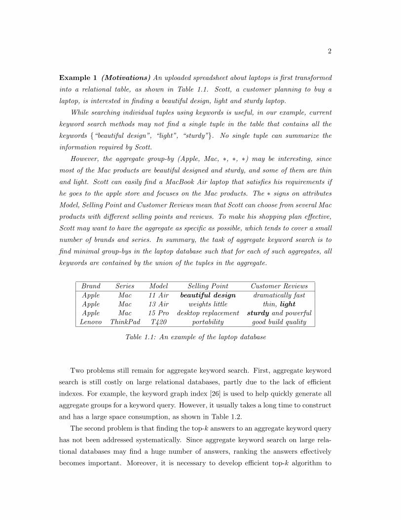
Example 1 (Motivations) An uploaded spreadsheet about laptops is first transformed
into a relational table, as shown in Table 1.1. Scott, a customer planning to buy a
laptop, is interested in finding a beautiful design, light and sturdy laptop.
While searching individual tuples using keywords is useful, in our example, current
keyword search methods may not find a single tuple in the table that contains all the
keywords “beautiful design”, “light”, “sturdy”. No single tuple can summarize the
information required by Scott.
However, the aggregate group-by (Apple, Mac, ∗, ∗, ∗) may be interesting, since
most of the Mac products are beautiful designed and sturdy, and some of them are thin
and light. Scott can easily find a MacBook Air laptop that satisfies his requirements if
he goes to the apple store and focuses on the Mac products. The ∗ signs on attributes
Model, Selling Point and Customer Reviews mean that Scott can choose from several Mac
products with different selling points and reviews. To make his shopping plan effective,
Scott may want to have the aggregate as specific as possible, which tends to cover a small
number of brands and series. In summary, the task of aggregate keyword search is to
find minimal group-bys in the laptop database such that for each of such aggregates, all
keywords are contained by the union of the tuples in the aggregate.
Brand Series Model Selling Point Customer Reviews
Apple Mac 11 Air beautiful design dramatically fastApple Mac 13 Air weights little thin, lightApple Mac 15 Pro desktop replacement sturdy and powerful
Lenovo ThinkPad T420 portability good build quality
Table 1.1: An example of the laptop database
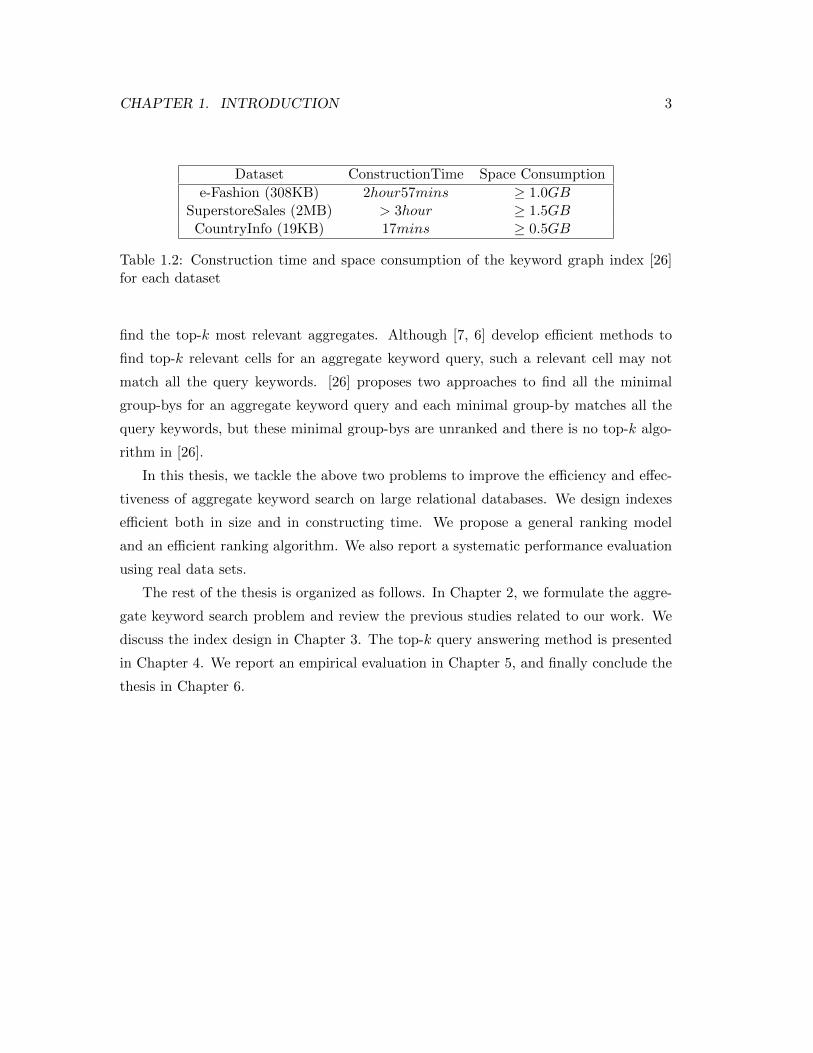
Two problems still remain for aggregate keyword search. First, aggregate keyword
search is still costly on large relational databases, partly due to the lack of efficient
indexes. For example, the keyword graph index [26] is used to help quickly generate all
aggregate groups for a keyword query. However, it usually takes a long time to construct
and has a large space consumption, as shown in Table 1.2.
The second problem is that finding the top-k answers to an aggregate keyword query
has not been addressed systematically. Since aggregate keyword search on large rela-
tional databases may find a huge number of answers, ranking the answers effectively
becomes important. Moreover, it is necessary to develop efficient top-k algorithm to
CHAPTER 1. INTRODUCTION 3
Dataset ConstructionTime Space Consumption
e-Fashion (308KB) 2hour57mins ≥ 1.0GBSuperstoreSales (2MB) > 3hour ≥ 1.5GB
CountryInfo (19KB) 17mins ≥ 0.5GB
Table 1.2: Construction time and space consumption of the keyword graph index [26]for each dataset
find the top-k most relevant aggregates. Although [7, 6] develop efficient methods to
find top-k relevant cells for an aggregate keyword query, such a relevant cell may not
match all the query keywords. [26] proposes two approaches to find all the minimal
group-bys for an aggregate keyword query and each minimal group-by matches all the
query keywords, but these minimal group-bys are unranked and there is no top-k algo-
rithm in [26].
In this thesis, we tackle the above two problems to improve the efficiency and effec-
tiveness of aggregate keyword search on large relational databases. We design indexes
efficient both in size and in constructing time. We propose a general ranking model
and an efficient ranking algorithm. We also report a systematic performance evaluation
using real data sets.
The rest of the thesis is organized as follows. In Chapter 2, we formulate the aggre-
gate keyword search problem and review the previous studies related to our work. We
discuss the index design in Chapter 3. The top-k query answering method is presented
in Chapter 4. We report an empirical evaluation in Chapter 5, and finally conclude the
thesis in Chapter 6.
Chapter 2
Problem Definition and Related
Work
For the sake of simplicity, we follow the terminology in [26] throughout the thesis. We
first review some basic concepts used in our aggregate keyword search model in Section
2.1, then formally state the problem in Section 2.2 and analyze the related works in
Section 2.3.
2.1 Preliminaries
We first review some definitions introduced in [26].
Definition 1 (Group-by, Cover, Base group-by, Ancestor and Descendant
[26]) Let T = (A1, · · · , An) be a relational table. A group-by on table T is a tuple
c = (x1, · · · , xn) where xi ∈ Ai or xi = ∗ (1 ≤ i ≤ n), and ∗ is a meta symbol meaning
that the attribute is generalized. The cover of group-by c is the set of tuples in T that
have the same values as c on those non-∗ attributes, that is, Cov(c) = (v1, · · · , vn) ∈T |vi = xi if xi 6= ∗, 1 ≤ i ≤ n .
A base group-by is a group-by which takes a non-∗ value on every attribute.
For two group-bys c1 = (x1, · · · , xn) and c2 = (y1, · · · , yn), c1 is an ancestor of c2,
and c2 a descendant of c1, denoted by c1 c2, if xi = yi for each xi 6= ∗(1 ≤ i ≤ n),
and there exists k(1 ≤ k ≤ n) such that xk = ∗ but yk 6= ∗.
The query model of aggregate keyword search on relational database in [26] is defined
as follows:
4
CHAPTER 2. PROBLEM DEFINITION AND RELATED WORK 5
Definition 2 (Aggregate keyword query) [26] Given a table T , an aggregate
keyword query is a 3-tuple Q = (D,C,W ), where D is a subset of attributes in table
T , C is a subset of text-rich attributes in T , and W is a set of keywords. We call D
the aggregate space and each attribute A ∈ D a dimension. We call C the set of
text attributes of Q. D and C do not have to be exclusive to each other.
In this thesis, we only consider short queries. So, we assume that the number of
keywords in each aggregate keyword query is small.
Definition 3 (Minimal Answer) [26] A group-by c is a minimal answer to an
aggregate keyword query Q if c is an answer to Q and every descendant of c is not an
answer to Q.
As mentioned in Chapter 1, users may prefer specific information, so our method
needs to guarantee that every returned group-by is minimal.
Definition 4 (Max-join) [26] For a set of tuples t1 and t2 in table T , the max-join
of t1 and t2 is a tuple t = “t1 ∨ t2” such that for any attribute A in T , t[A] = t1[A] if
t1[A] = t2[A], otherwise t[A] = ∗. We call (∗, ∗, · · · , ∗) a trivial answer.
Lemma 1 (Max-join on answers) [26] If t is a minimal answer to aggregate key-
word query Q = (D,C, w1, · · · , wm), then there exists minimal answers t1 and t2 to
queries (D,C, w1,w2) and (D,C, w2,· · · , wm), respectively, such that t = t1 ∨ t2.
According to Lemma 1, if we already know answers Ans1 for (D,C, w1, w2)and answers Ans2 for (D,C, w2, · · · , wm), we can generate answers for query Q =
(D,C, w1, · · · , wm) by performing max-join on Ans1 and Ans2. For example, if
t1 ∈ Ans1 and t2 ∈ Ans2, we can get an answer t = t1 ∨ t2 for query Q.
The retrieval model of aggregate keyword search on relational databases in [26] :
given an aggregate query Q=(D,C, w1, · · · ,wm), it first performs max-join on each
pair of rows in the database to get a set of answers Ans1,Ans2, . . . , Ansm−1 for
(D,C, w1,w2), (D,C, w2,w3), . . . , (D,C, wm−1, wm); using Lemma 1 repeatedly,
answers for query Q can then be generated by performing max-join on Ans1,Ans2, . . . ,
Ansm−1.
Proof 1 [26] Since t is a minimal answer, there must exist one group-by (based on t)
that has tuples matching w1, w2, · · · , wm. This group-by also matches w1, w2 and
2.1. PRELIMINARIES 6
w2, · · · , wm as well. Thus, there must exist minimal answers t1 and t2 for queries
w1, w2 and w2, · · · , wm, and t1 and t2 may be equal to t, or t1 and t2 may be a
descendant of t. So t1 ∨ t2 could be equal to t, or t1 ∨ t2 could be a descendant of t. The
latter one is not possible, since t is a minimal answer (because t1 ∨ t2 is also an answer
to w1, w2, · · · , wm).
Property 1 [26] To answer query Q = (D,C, w1, · · · , wm), using Lemma 1 repeat-
edly, we only need to check m− 1 edges covering all keywords w1, · · · , wm in the clique.
Each edge is associated with the set of minimal answers to a query on a pair of keywords.
The weight of the edge is the size of the answer set. In order to reduce the total cost of
the joins, heuristically, we can find a spanning tree connecting the m keywords such that
the product of the weights on the edges is minimized.
Definition 5 (Keyword Graph Index) [26] Given a table T , a keyword graph
index is an undirected graph G(T ) = (V,E) such that 1) V is the set of keywords in
the table T ; and 2) (u, v) ∈ E is an edge if there exists a non-trivial answer to query
Quv = (D,C, u, v). Edge (u, v) is associated with the set of minimal answers to query
Quv.
Zhou and Pei [26] proved that 1) if there exists a nontrivial answer to an aggre-
gate keyword query Q, the keyword graph index exists a clique on all keywords of Q
(Theorem 3 in [26]).
We define the query keyword graph as follows.
Definition 6 (Query Keyword Graph) Given a table T , a query keyword graph
for the aggregate keyword query Q is an undirected graph G(T,Q) = (V , E) such that
1) V is the set of query keywords in Q =(D,C,w1,· · · ,wm) ; and 2) (wi, wj) ∈ E is
an edge if there exists a non-trivial answer to query (D,C, wi, wj), Edge (wi, wj) is
associated with the set of minimal answers to query (D,C,wi, wj), 1 ≤ i, j ≤ m.
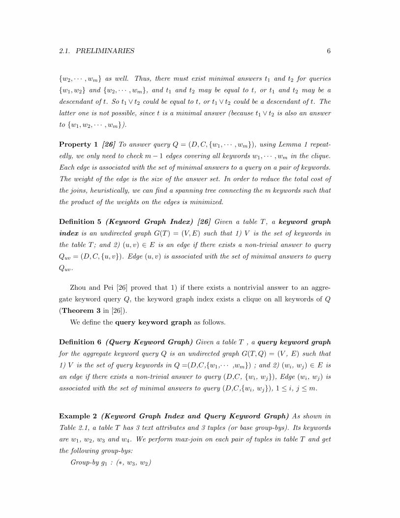
Example 2 (Keyword Graph Index and Query Keyword Graph) As shown in
Table 2.1, a table T has 3 text attributes and 3 tuples (or base group-bys). Its keywords
are w1, w2, w3 and w4. We perform max-join on each pair of tuples in table T and get
the following group-bys:
Group-by g1 : (∗, w3, w2)
CHAPTER 2. PROBLEM DEFINITION AND RELATED WORK 7
RowID TextAttri1 TextAttri2 TextAttri3r1 w1 w3 w2
r2 w4 w3 w2
r3 w1 w3 w4
Table 2.1: An example of table T
Group-by g2 : (w1, w3, ∗)Group-by g3 : (∗, w3, ∗)Base Group-by r1 : (w1, w3, w2)
Base Group-by r2: (w4, w3, w2)
Base Group-by r3: (w1, w3, w4)
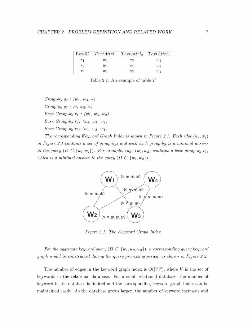
The corresponding Keyword Graph Index is shown in Figure 2.1. Each edge (wi, wj)
in Figure 2.1 contains a set of group-bys and each such group-by is a minimal answer
to the query (D,C, wi, wj). For example, edge (w1, w2) contains a base group-by r1,
which is a minimal answer to the query (D,C, w1, w2).
Figure 2.1: The Keyword Graph Index
For the aggregate keyword query (D,C, w1, w2, w3), a corresponding query keyword
graph would be constructed during the query processing period, as shown in Figure 2.2.
The number of edges in the keyword graph index is O(|V |2), where V is the set of
keywords in the relational database. For a small relational database, the number of
keyword in the database is limited and the corresponding keyword graph index can be
maintained easily. As the database grows larger, the number of keyword increases and

2.2. PROBLEM STATEMENT AND SOLUTION 8
Figure 2.2: The Query Keyword Graph
the keyword graph index becomes less efficient.
The difference between the query keyword graph and the keyword graph index is
that vertices of the former are keywords in the query Q and vertices of the latter are
keywords in the database.
Since the number of keywords in a query is much smaller than the number of key-
words in a relational database, the query keyword graph is much smaller than the
keyword graph index [26] and can be constructed quickly.
Theorem 1 (Query Keyword Graph) For an aggregate keyword query Q , there
exists a non-trivial answer to Q in table T only if in the query keyword graph G(T,Q)
is a clique.
Proof 2 Let c be a non-trivial answer to Q = (D,C,W ). Then, for any u, v ∈ W , c
must be a non-trivial answer to query Qu,v = (D,C, u, v). That is, (u, v) is an edge
in G(T,Q).
2.2 Problem Statement and Solution
2.2.1 Indexing
As discussed in Section 2.1, the number of edges in the keyword graph index on a
relational database is O(|V |2), where V is the set of keywords in the database. As the
database grows larger, the number of keyword increases and the keyword graph index
becomes less efficient. Table 1.2 shows the sizes, as well as the constructing times of
three keyword graph indexes on different datasets.
CHAPTER 2. PROBLEM DEFINITION AND RELATED WORK 9
Our solution is to build a new index, such that its stored information can be used
to construct a query keyword graph during the query-processing period. The aggregate
information in the query keyword graph is then used to generate minimal answers. If
the query contains m keywords, to construct the query keyword graph, we need build
m− 1 edges. The construction time of the query keyword graph grows linearly with the
number of keywords in the query. Since we assume that the number of keywords in a
query is small, the query keyword graph is very small and can be constructed quickly.
Our complete query-answering method successfully uses the new index to generate
all the minimal answers to a keyword query.
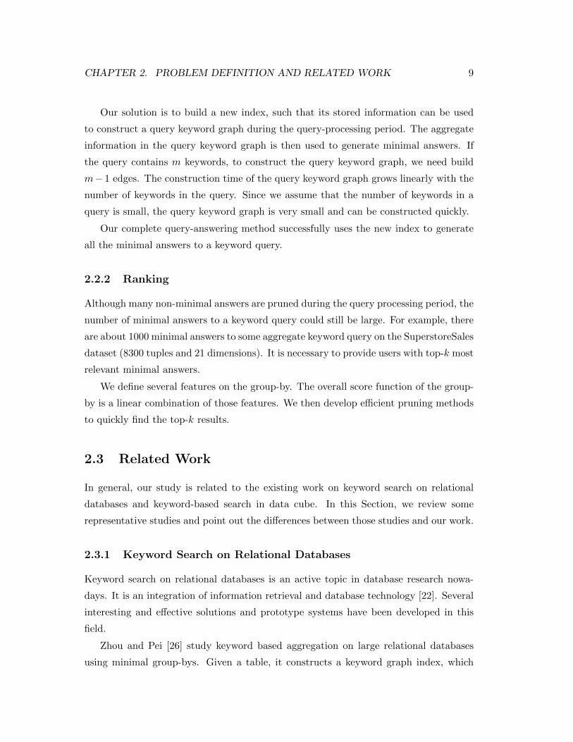
2.2.2 Ranking
Although many non-minimal answers are pruned during the query processing period, the
number of minimal answers to a keyword query could still be large. For example, there
are about 1000 minimal answers to some aggregate keyword query on the SuperstoreSales
dataset (8300 tuples and 21 dimensions). It is necessary to provide users with top-k most
relevant minimal answers.
We define several features on the group-by. The overall score function of the group-
by is a linear combination of those features. We then develop efficient pruning methods
to quickly find the top-k results.
2.3 Related Work
In general, our study is related to the existing work on keyword search on relational
databases and keyword-based search in data cube. In this Section, we review some
representative studies and point out the differences between those studies and our work.
2.3.1 Keyword Search on Relational Databases
Keyword search on relational databases is an active topic in database research nowa-
days. It is an integration of information retrieval and database technology [22]. Several
interesting and effective solutions and prototype systems have been developed in this
field.
Zhou and Pei [26] study keyword based aggregation on large relational databases
using minimal group-bys. Given a table, it constructs a keyword graph index, which
2.3. RELATED WORK 10
would be used during the online query processing period to generate all minimal answers
that contain all the user given keywords. Each edge in the keyword graph index is
corresponding to a pair of keywords. Minimal answers to every pair of keywords are
pre-calculated and stored in the keyword graph index. To answer an aggregate keyword
query Q, it first scans the keyword graph index to check if there exists a clique on all
the query keywords. If so, it then performs max-join repeatedly on |Q| − 1 edges in
that clique and finds nontrivial minimal answers from the max-join results. If not, there
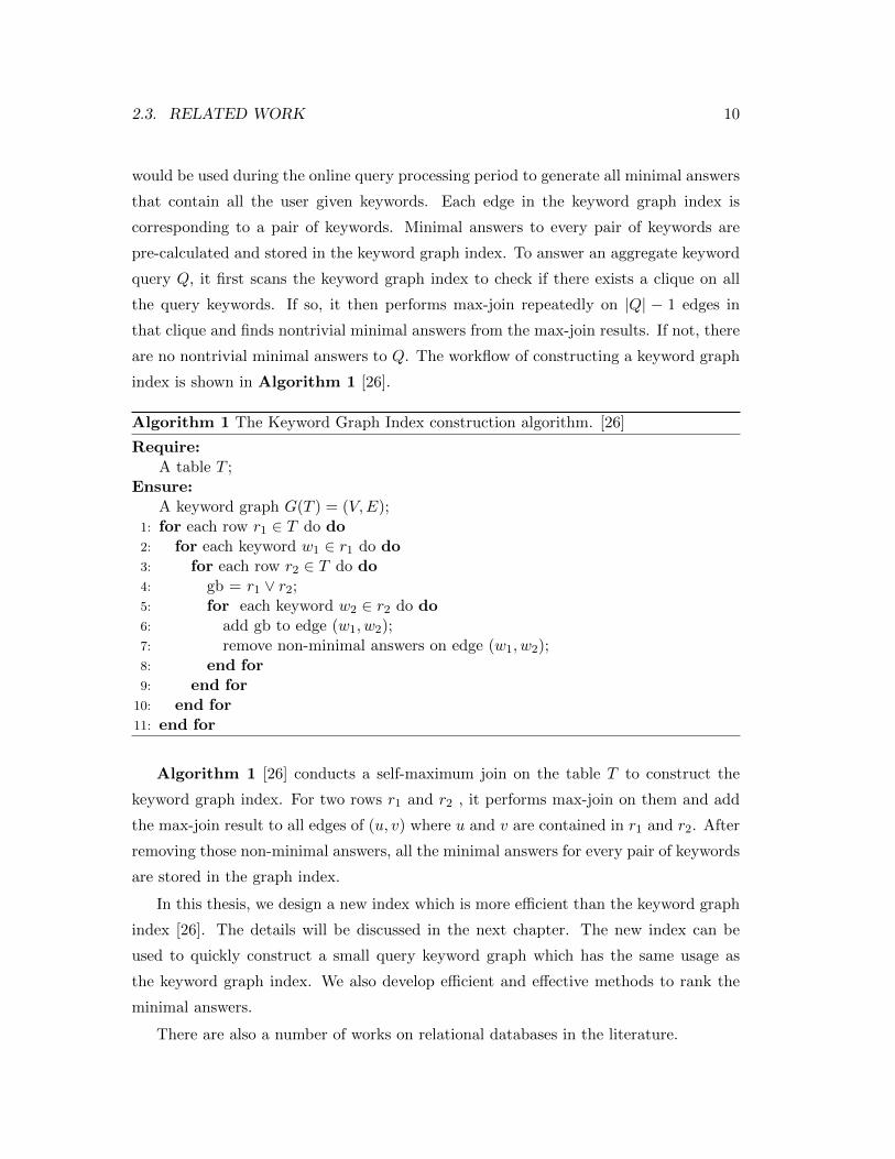
are no nontrivial minimal answers to Q. The workflow of constructing a keyword graph
index is shown in Algorithm 1 [26].
Algorithm 1 The Keyword Graph Index construction algorithm. [26]
Require:A table T ;
Ensure:A keyword graph G(T ) = (V,E);
1: for each row r1 ∈ T do do2: for each keyword w1 ∈ r1 do do3: for each row r2 ∈ T do do4: gb = r1 ∨ r2;5: for each keyword w2 ∈ r2 do do6: add gb to edge (w1, w2);7: remove non-minimal answers on edge (w1, w2);8: end for9: end for
10: end for11: end for
Algorithm 1 [26] conducts a self-maximum join on the table T to construct the
keyword graph index. For two rows r1 and r2 , it performs max-join on them and add
the max-join result to all edges of (u, v) where u and v are contained in r1 and r2. After
removing those non-minimal answers, all the minimal answers for every pair of keywords
are stored in the graph index.
In this thesis, we design a new index which is more efficient than the keyword graph
index [26]. The details will be discussed in the next chapter. The new index can be
used to quickly construct a small query keyword graph which has the same usage as
the keyword graph index. We also develop efficient and effective methods to rank the
minimal answers.
There are also a number of works on relational databases in the literature.

CHAPTER 2. PROBLEM DEFINITION AND RELATED WORK 11
Balmin et al. [2] treat the database as a labeled graph. It builds a labeled graph
index which has a natural flow of authority. For example, to generate a labeled graph
index on the DBLP database, 1) it extracts some labels (conference, year, paper and
author) from the DBLP database; 2) a schema graph is built based on the relationships
of these labels, as shown in Figure 2.3; and 3) the labeled graph index is obtained
by annotating the schema graph, Figure 2.4 shows a subset of the labeled graph on the
DBLP database. Given a keyword query, Balmin et al. [2] applies a PageRank algorithm
to find nodes (in the labels graph) that have high authority with respect to all query
keywords.
Figure 2.3: The DBLP schema graph [2]
Figure 2.4: A subset of the DBLP graph [2]
The index in Hristidis et al. [12] is combined of a set of joining networks, each
2.3. RELATED WORK 12
represents a row that could be generated by joining rows in multiple tables using primary
and foreign keys. Given a keyword query, it scans the index to find relevant joining
networks such that each relevant joining network contains all the query keywords.
Agrawal et al. [1] implements a keyword-based search system (DBXplorer) on a
commercial database. Such a system returns relevant rows as answers such that each
relevant row contains all the query keywords. Its index contains a symbol table which
can help to quickly locate the query keywords in the relational database.
Bhalotia et al. [4] designs a graph index on the database. Each node represents a
row and each edge represents an application-oriented relationship of two rows. Given a
keyword query, it scans the index to find Steiner trees [11] that contain all the query
keywords.
These previous studies [2, 12, 1, 4] focus on finding relevant tuples instead of aggre-
gate cells, so their indexes, score functions and top-k algorithms can hardly be extended
to solve our problems.
2.3.2 Keyword-based search in data cube
In data cubes built on top of databases, B. Ding et al. [7, 6] find the top-k most
relevant cells for a keyword query, while B. Zhao itet al. [25] and Wu et al. [24] support
interactive exploration of data using keyword search.
B. Ding et al. [7, 6] study the keyword search problem on data cube with text-rich
dimensions, which is the work most relevant to ours. They rank cells within the data
cube of a database according to their relevance for the query q. The relevance score
of a cell Ccell is defined as a function rel(q, Ccell) of the cell document Ccell[Dcell] and
the query q. In their work, a base group-by is treated as a document and documents
covered by a cell Ccell is treated as a “big document” (also called cell document of Ccell,
represented by Ccell[Dcell]). The relevance score of the cell Ccell is the relevance of this
big document with respect to q. In summary, they use an IR style model to design the
score function of a cell.
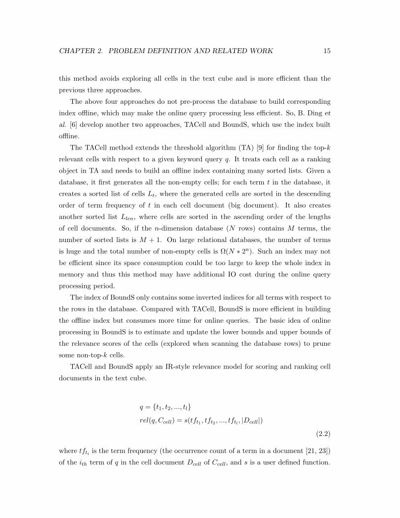
The score function used in [7] is as follows:
rel(q, Ccell) =∑t∈q
lnN − dft + 0.5
dft + 0.5
(k1 + 1)tft,Dcell
k1((1− b) + b dlDavdl ) + tft,Dcell
(k3 + 1)qtft,qk3 + qtft,q
(2.1)
CHAPTER 2. PROBLEM DEFINITION AND RELATED WORK 13
where N is the number of rows in the database, Dcell is the big document of Ccell,
tft,Dcellis the term frequency of term t ∈ q in Dcell , dft is the number of documents in
the database containing t, dlD represents the length of Dcell, avdl is the average length
of documents covered by Ccell, qtft,q is the number of times t appearing in q, and k1,b,
k3 are the parameters used in Okapi BM25 [20, 19].
Since the parameters of Okapi BM25 are query- and collection (cell) -dependent, this
score function may suffer from the problem of tuning parameters.
To find the top-k relevant cells, B. Ding proposes four approaches in [7]: inverted-
index one-scan, document sorted-scan, bottom-up dynamic programming, and search-
space ordering. In [6], another two approaches are proposed: TACell and BoundS.
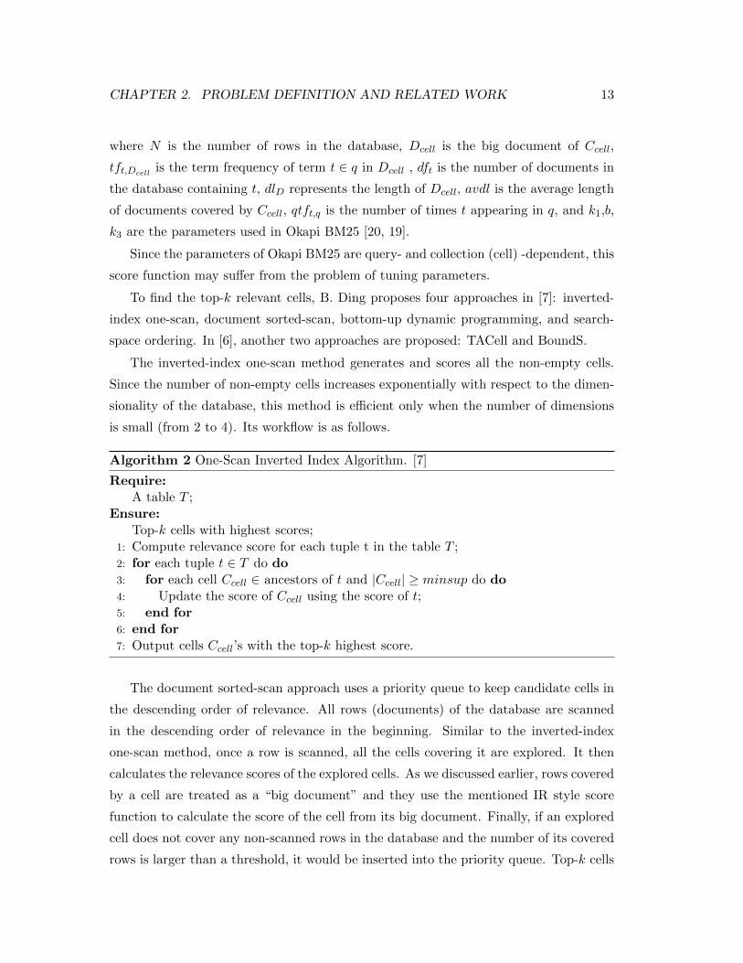
The inverted-index one-scan method generates and scores all the non-empty cells.
Since the number of non-empty cells increases exponentially with respect to the dimen-
sionality of the database, this method is efficient only when the number of dimensions
is small (from 2 to 4). Its workflow is as follows.
Algorithm 2 One-Scan Inverted Index Algorithm. [7]
Require:A table T ;
Ensure:Top-k cells with highest scores;
1: Compute relevance score for each tuple t in the table T ;2: for each tuple t ∈ T do do3: for each cell Ccell ∈ ancestors of t and |Ccell| ≥ minsup do do4: Update the score of Ccell using the score of t;5: end for6: end for7: Output cells Ccell’s with the top-k highest score.
The document sorted-scan approach uses a priority queue to keep candidate cells in
the descending order of relevance. All rows (documents) of the database are scanned
in the descending order of relevance in the beginning. Similar to the inverted-index
one-scan method, once a row is scanned, all the cells covering it are explored. It then
calculates the relevance scores of the explored cells. As we discussed earlier, rows covered
by a cell are treated as a “big document” and they use the mentioned IR style score
function to calculate the score of the cell from its big document. Finally, if an explored
cell does not cover any non-scanned rows in the database and the number of its covered
rows is larger than a threshold, it would be inserted into the priority queue. Top-k cells
2.3. RELATED WORK 14
are selected from the priority queue. For this method, once a row is scanned, 2n cells
are explored in a n-dimension cube. So the numbers of candidate cells and explored
cells increase very quickly. Although the complexity of this method is worse than the
inverted-index one-scan, it may terminate earlier before scanning all rows.
Different from the above one-scan and sorted-scan approaches which compute the
relevance score of a cell from rows in the database, the bottom-up approach and the
search-space ordering approach compute the score of a cell from its children cells in a
dynamic-programming manner. The following example shows the relationship of a cell
Ccell and its children cells.
Example 3 Given a database with 3 dimensions, suppose the first dimension only con-
tains 2 unique values “x1” and “x2” in the database, if Ccell = (∗, ∗, x3), C1 = (x1, ∗, x3)and C2 = (x2, ∗, x3) (C1 and C2 are the children of Ccell), we can quickly find out that
Cov(Ccell) = Cov(C1) + Cov(C2). So, we have two properties:
Property 2 The score of cell Ccell can be easily computed from the scores of C1 and
C2.
Property 3 For any non-base cell Ccell in text cube and any query q, there exists two
children Ci and Cj of Ccell such that rel(q, Ci) ≤ rel(q, Ccell) ≤ rel(q, Cj). The proof is
given in Section 3 of [7].
The bottom-up approach is based on a dynamic programming algorithm which di-
rectly utilizes property 2. The algorithm first computes the relevance scores rel(q, Ccell)
for all rows (n-dimension base cells). By using property 2, it then computes the rele-
vance scores from the base cells to higher levels. Finally, after the relevance scores of
all cells are obtained, it outputs the top-k relevant ones with supports no less than a
threshold. Since the score of a cell on a certain level can be quickly calculated from its
children cells on the lower level, which is faster than computing from cells on the base
level, the bottom-up is more efficient than the previous two approaches. However, the
bottom-up method still needs to calculate the scores of all the cells, so it’s efficient only
when the number of dimensions is small.
The search-space ordering method carries out cell-based search and explores as small
number of cells in the cube as possible to find the top-k answers. Property 2 and property
3 are utilized in this method. Since the search space can be pruned using property 3,
CHAPTER 2. PROBLEM DEFINITION AND RELATED WORK 15
this method avoids exploring all cells in the text cube and is more efficient than the
previous three approaches.
The above four approaches do not pre-process the database to build corresponding
index offline, which may make the online query processing less efficient. So, B. Ding et
al. [6] develop another two approaches, TACell and BoundS, which use the index built
offline.
The TACell method extends the threshold algorithm (TA) [9] for finding the top-k
relevant cells with respect to a given keyword query q. It treats each cell as a ranking
object in TA and needs to build an offline index containing many sorted lists. Given a
database, it first generates all the non-empty cells; for each term t in the database, it
creates a sorted list of cells Lt, where the generated cells are sorted in the descending
order of term frequency of t in each cell document (big document). It also creates
another sorted list Llen, where cells are sorted in the ascending order of the lengths
of cell documents. So, if the n-dimension database (N rows) contains M terms, the
number of sorted lists is M + 1. On large relational databases, the number of terms
is huge and the total number of non-empty cells is Ω(N ∗ 2n). Such an index may not
be efficient since its space consumption could be too large to keep the whole index in
memory and thus this method may have additional IO cost during the online query
processing period.
The index of BoundS only contains some inverted indices for all terms with respect to
the rows in the database. Compared with TACell, BoundS is more efficient in building
the offline index but consumes more time for online queries. The basic idea of online
processing in BoundS is to estimate and update the lower bounds and upper bounds of
the relevance scores of the cells (explored when scanning the database rows) to prune
some non-top-k cells.
TACell and BoundS apply an IR-style relevance model for scoring and ranking cell
documents in the text cube.
q = t1, t2, ..., tl
rel(q, Ccell) = s(tft1 , tft2 , ..., tftl , |Dcell|)
(2.2)
where tfti is the term frequency (the occurrence count of a term in a document [21, 23])
of the ith term of q in the cell document Dcell of Ccell, and s is a user defined function.

2.3. RELATED WORK 16
The score function s() needs to be monotone to ensure the correctness of TACell and
BoundS. B. Ding et al. [6] use a simple monotone function which considers the term
frequency and document length (terminology in IR). If more IR features (such as dft
and qtft,q) are considered in the score function, 1) more sorted lists need to be created
in TACell and thus its index would have an even larger space consumption; and 2) the
upper bounds and lower bounds defined in BoundS may no longer be applicable.
In BoundS, B. Ding et al. [6] assume that the length of each cell’s big document
(document length) is precomputed, so B. Ding et al. [6] only need to consider the
term frequency when estimating the lower bounds and upper bounds of the relevance
scores of the cells. In such a case, if more rows are scanned, the number of times a
query term appear in a cell’s big document will possibly increase. Then, bounds can
be estimated since the score function is monotonically increasing with respect to the
term frequency. If more IR features are considered in the score function, the score of
a cell may decrease when more rows are scanned. Moreover, if the score function only
considers term frequency and document length, the query processing time may be short
but the quality of the top-k cells may not be guaranteed.
Wu et al. [24] propose a system (KDAP) which supports interactive exploration of
data using keyword search. Given a keyword query, the system first generates the candi-
date subspaces in an OLAP database such that each subspace essentially corresponds to
a possible join path between the dimensions and the facts. It then ranks the subspaces
and asks users to select one subspace. Finally, it computes the group-by aggregates over
some predefined measure using qualified fact points in the selected subspace and finds
the top-k group-by attributes to partition the subspace.
B. Zhao et al. [25] propose a similar keyword-based interactive exploration frame-
work called TEXplorer. Different from the work in [26, 7, 6], whose goal is to return a
ranked list of the cells directly, TEXplorer guides users to find their interested informa-
tion step by step.
Given a keyword query q and a table T , TEXplorer first calculates the significance of
each dimension of the table T using a novel significance measure. A user then determine
which dimension to drill down. Once the user drill down a certain dimension, cells in the
corresponding cuboid are ranked by using the following equation. The user can select
an interested cell Ccell from a list of ranked cells in that cuboid.

CHAPTER 2. PROBLEM DEFINITION AND RELATED WORK 17
Rel(q, Ccell) =1
|Dcell|∑
d∈Dcell
rel(q, d)
rel(q, d) =∑w∈q
IDFw ∗ TFWw,dQTWw,q
(2.3)
where Dcell represents the cell documents (terminology in [7, 6]) of cell Ccell , rel(q, d)
is the relevance of a document d (a row is treated as a document ) with respect to q,
IDFw is the inverted document frequency factor of term w ∈ q, TFWw,d represents the
term frequency factor of w in document d, and QTWw,q is the query term frequency
factor of w in q.
In the second stage of TEXplorer, the rest dimensions and cells in each dimension
are re-ranked based on the selected cell Ccell. Users can repeat to drill down another
dimension and select a cell (a child of cell Ccell) in the corresponding cuboid. Figure 2.5
is a running example of TEXplorer in [25]. It shows how a user uses the TEXplorer to
find a powerful laptop suitable for gaming step by step.
Figure 2.5: Keyword-based interactive exploration in TEXplorer [25]
In TEXplorer, the significance of a dimension Ai is measured by CVAi and IDVAi ,
as shown in Equation 2.4. The CV function measures how much the relevance of each
of Ccell’s Ai-children deviates from the relevance of Ccell. For instance, in [25], given
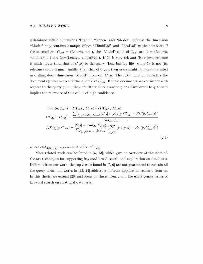
2.3. RELATED WORK 18
a database with 3 dimensions “Brand”, “Screen” and “Model”, suppose the dimension
“Model” only contains 2 unique values “ThinkPad” and “IdeaPad” in the database. If
the selected cell Ccell = (Lenovo, ∗,∗ ), the “Model”-child of Ccell are C1= (Lenovo,
∗,ThinkPad ) and C2=(Lenovo, ∗,IdeaPad ). If C1 is very relevant (its relevance score
is much larger than that of Ccell) to the query “long battery life” while C2 is not (its
relevance score is much smaller than that of Ccell), then users might be more interested
in drilling down dimension “Model” from cell Ccell. The IDV function considers the
documents (rows) in each of the Ai-child of Ccell. If these documents are consistent with
respect to the query q, i.e., they are either all relevant to q or all irrelevant to q, then it
implies the relevance of this cell is of high confidence.
SigAi(q, Ccell) = CVAi(q, Ccell) ∗ IDVAi(q, Ccell)
CVAi(q, Ccell) =
∑C′
cell∈chdAi(Ccell)
|C ′D| ∗ (Rel(q, C ′cell)−Rel(q, Ccell))2
|chdAi(Ccell)| − 1
IDVAi(q, Ccell) =|CD| − |chdAi(Ccell)|∑
C′cell∈chd(Ai)
(Ccell)(∑d∈C′
D
(rel(q, d)−Rel(q, C ′cell))2)
(2.4)
where chdAi(Ccell) represents Ai-child of Ccell.
More related work can be found in [5, 13], which give an overview of the state-of-
the-art techniques for supporting keyword-based search and exploration on databases.
Different from our work, the top-k cells found in [7, 6] are not guaranteed to contain all
the query terms and works in [25, 24] address a different application scenario from us.
In this thesis, we extend [26] and focus on the efficiency and the effectiveness issues of
keyword search on relational databases.
Chapter 3
The Efficient Index
Without building any index on a relational database, we need to scan the whole database
online to generate all the minimal group-bys for an aggregate keyword query. There is
no problem if the queries are very long. However, as mentioned in Chapter 2, we only
consider short queries. In such a case, building index can make the aggregate keyword
search more efficient.
As the relational database grows larger, the keyword graph index [26] may a high
space consumption and thus requires additional IO operations when memory is not
large enough during the query processing period. To make aggregate keyword search
more efficient on large relational databases, we design a new index, which is smaller and
faster to construct. The new index can be used to correctly generate the same minimal
aggregates as the keyword graph index [26]. We test the new index in the complete
query answering method.
3.1 Introduction
As discussed in Chapter 2, Zhou and Pei [26] materialized a keyword graph index for
fast answering of keyword queries on relational databases.
To help quickly generate minimal answers for a keyword query, minimal answers to
every pair of keywords are pre-calculated and stored in the keyword graph index. In
other words, for any query that contains only two keywords w1 and w2, the minimal
answers can be found directly from edge (w1, w2) since the answers are materialized on
the edge. If the query involves more than 2 keywords and there exists a clique on all
the query keywords in the keyword graph index, the minimal answers can be computed
19
3.2. THE NEW INDEX 20
by performing maximum joins on the sets of minimal answers associated with the edges
in the clique. So, storing all the minimal answers for each pair of keywords is useful for
fast answering of keyword search on relational databases. However, the disadvantage is
that it leads to an increase in the space consumption of the keyword graph index.
The number of edges in the keyword graph index is proportional to the square of the
number of keywords in the relational database. If the database grows larger or becomes
text-richer, the keyword graph index could contain huge number of edges and thus has
a high space consumption.
Example 4 (Space Consumption of the Keyword Graph Index) Given a table
T with m = 104 unique keywords and n = 10 dimensions, the number of edges in
the corresponding keyword graph index is n1 = m×(m−1)2 = 0.5 × 10⁸. If the average
number of minimal answers on each edge is p = 5, the keyword graph index contains
n2 = n1 × p = 2.5× 10⁸ minimal answers. If we use an integer (4 bytes) to represent a
dimension value, the size of a minimal answer is p′ = n × 4 = 40 bytes, so the size of
the keyword graph index is p′ × n2 = 1010 bytes, which is about 10 GB.
Although the size of the keyword graph index can be decreased if we store all gen-
erated group-bys in a set (to prune duplicated group-bys) and replace each group-by in
the graph with its position in this set, the space consumption is still a bottleneck and
we need to design more efficient index for large relational databases. Such a new index
should have less space consumption and can still help quickly generate minimal answers
for a keyword query.
3.2 The new index
Our new index is called Inverted Pair-wise Joins (IPJ), which is designed based on the
following idea:
The index only needs to store necessary information that can be used to quickly
generate the same clique as is used in the keyword graph index [26] during the query
processing period.
3.2.1 Definitions
Definition 7 Given a table T , an index is constructed such that:
CHAPTER 3. THE EFFICIENT INDEX 21
• The Pair-wise Joins of a keyword w PJ [w]= gb | gb is a group-by such that
gb = ri ∨ rj, where w is a keyword in T , (ri, rj) is a pair of rows in T , w ∈ ri or
w ∈ rj
• The Inverted Pair-wise Joins IPJ= (w,PJ [w]) | w is a keyword in the table
T
For each keyword w in the table, the inverted pair-wise joins IPJ records the cor-
responding pair-wise joins of w (PJ [w]). PJ [w] stores without redundancy all relevant
group-bys (non-trivial) such that each relevant group-by is generated by performing
max-join operation on a certain pair of rows (at least one row contains the keyword w).
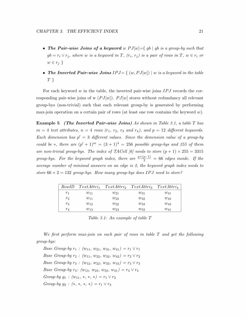
Example 5 (The Inverted Pair-wise Joins) As shown in Table 3.1, a table T has
m = 4 text attributes, n = 4 rows (r1, r2, r3 and r4), and p = 12 different keywords.
Each dimension has p′ = 3 different values. Since the dimension value of a group-by
could be ∗, there are (p′ + 1)m = (3 + 1)4 = 256 possible group-bys and 255 of them
are non-trivial group-bys. The index of TACell [6] needs to store (p + 1) × 255 = 3315
group-bys. For the keyword graph index, there are p×(p−1)2 = 66 edges inside. If the
average number of minimal answers on an edge is 2, the keyword graph index needs to
store 66× 2 = 132 group-bys. How many group-bys does IPJ need to store?
RowID TextAttri1 TextAttri2 TextAttri3 TextAttri4r1 w11 w21 w31 w41
r2 w11 w22 w32 w42
r3 w12 w22 w33 w43
r4 w13 w23 w33 w41
Table 3.1: An example of table T
We first perform max-join on each pair of rows in table T and get the following
group-bys:
Base Group-by r1 : (w11, w21, w31, w41) = r1 ∨ r1Base Group-by r2 : (w11, w22, w32, w42) = r2 ∨ r2Base Group-by r3 : (w12, w22, w33, w43) = r3 ∨ r3Base Group-by r4: (w13, w23, w33, w41) = r4 ∨ r4Group-by g1 : (w11, ∗, ∗, ∗) = r1 ∨ r2Group-by g2 : (∗, ∗, ∗, ∗) = r1 ∨ r3
3.2. THE NEW INDEX 22
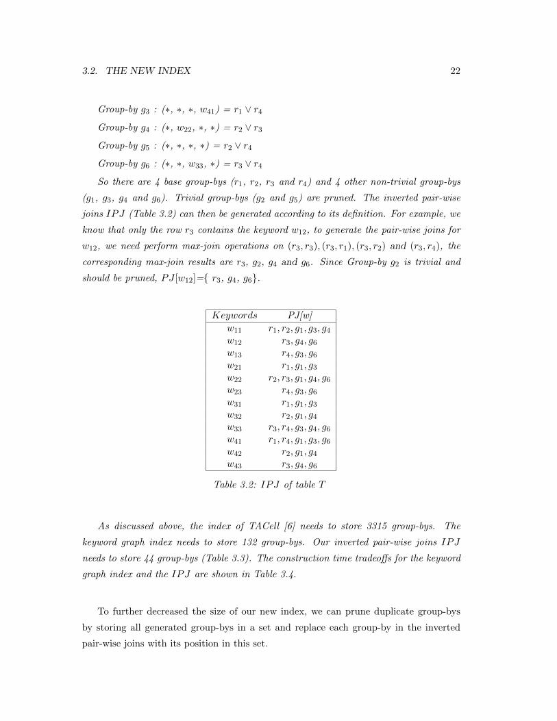
Group-by g3 : (∗, ∗, ∗, w41) = r1 ∨ r4Group-by g4 : (∗, w22, ∗, ∗) = r2 ∨ r3Group-by g5 : (∗, ∗, ∗, ∗) = r2 ∨ r4Group-by g6 : (∗, ∗, w33, ∗) = r3 ∨ r4So there are 4 base group-bys (r1, r2, r3 and r4) and 4 other non-trivial group-bys
(g1, g3, g4 and g6). Trivial group-bys (g2 and g5) are pruned. The inverted pair-wise
joins IPJ (Table 3.2) can then be generated according to its definition. For example, we
know that only the row r3 contains the keyword w12, to generate the pair-wise joins for
w12, we need perform max-join operations on (r3, r3), (r3, r1), (r3, r2) and (r3, r4), the
corresponding max-join results are r3, g2, g4 and g6. Since Group-by g2 is trivial and
should be pruned, PJ [w12]= r3, g4, g6.
Keywords PJ[w]
w11 r1, r2, g1, g3, g4w12 r3, g4, g6w13 r4, g3, g6w21 r1, g1, g3w22 r2, r3, g1, g4, g6w23 r4, g3, g6w31 r1, g1, g3w32 r2, g1, g4w33 r3, r4, g3, g4, g6w41 r1, r4, g1, g3, g6w42 r2, g1, g4w43 r3, g4, g6
Table 3.2: IPJ of table T
As discussed above, the index of TACell [6] needs to store 3315 group-bys. The
keyword graph index needs to store 132 group-bys. Our inverted pair-wise joins IPJ
needs to store 44 group-bys (Table 3.3). The construction time tradeoffs for the keyword
graph index and the IPJ are shown in Table 3.4.
To further decreased the size of our new index, we can prune duplicate group-bys
by storing all generated group-bys in a set and replace each group-by in the inverted
pair-wise joins with its position in this set.
CHAPTER 3. THE EFFICIENT INDEX 23
TACell Index [6] KeywordGraphIndex [26] IPJ
3315 132 44
Table 3.3: Number of group-bys in different indexes
3.2.2 How to use the new index?
To capture our intuition, we define the inverted pair-wise joins and test it in our complete
query-answering method.
To answer the query q = (D,C, w1, · · · , wh), the complete query-answering method
first constructs a query keyword graph (Section 2.1) by using our new index.
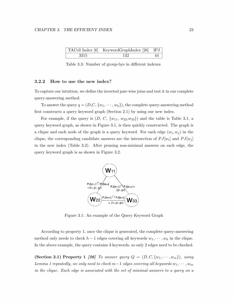
For example, if the query is (D, C, w11, w22,w33) and the table is Table 3.1, a
query keyword graph, as shown in Figure 3.1, is then quickly constructed. The graph is
a clique and each node of the graph is a query keyword. For each edge (wi, wj) in the
clique, the corresponding candidate answers are the intersection of PJ [wi] and PJ [wj ]
in the new index (Table 3.2). After pruning non-minimal answers on each edge, the
query keyword graph is as shown in Figure 3.2.
Figure 3.1: An example of the Query Keyword Graph
According to property 1, once the clique is generated, the complete query-answering
method only needs to check h− 1 edges covering all keywords w1, · · · , wh in the clique.
In the above example, the query contains 3 keywords, so only 2 edges need to be checked.
(Section 2.1) Property 1 [26] To answer query Q = (D,C, w1, · · · , wm), using
Lemma 1 repeatedly, we only need to check m−1 edges covering all keywords w1, · · · , wm
in the clique. Each edge is associated with the set of minimal answers to a query on a
3.2. THE NEW INDEX 24
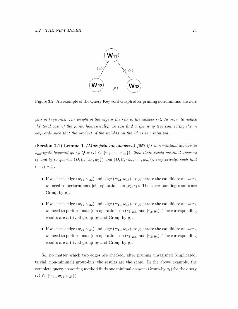
Figure 3.2: An example of the Query Keyword Graph after pruning non-minimal answers
pair of keywords. The weight of the edge is the size of the answer set. In order to reduce
the total cost of the joins, heuristically, we can find a spanning tree connecting the m
keywords such that the product of the weights on the edges is minimized.
(Section 2.1) Lemma 1 (Max-join on answers) [26] If t is a minimal answer to
aggregate keyword query Q = (D,C, w1, · · · , wm), then there exists minimal answers
t1 and t2 to queries (D,C, w1, w2) and (D,C, we, · · · , wm), respectively, such that
t = t1 ∨ t2.
• If we check edge (w11, w22) and edge (w22, w33), to generate the candidate answers,
we need to perform max-join operations on (r2, r3). The corresponding results are
Group-by g4.
• If we check edge (w11, w22) and edge (w11, w33), to generate the candidate answers,
we need to perform max-join operations on (r2, g3) and (r2, g4). The corresponding
results are a trivial group-by and Group-by g4.
• If we check edge (w22, w33) and edge (w11, w33), to generate the candidate answers,
we need to perform max-join operations on (r3, g3) and (r3, g4). The corresponding
results are a trivial group-by and Group-by g4.
So, no matter which two edges are checked, after pruning unsatisfied (duplicated,
trivial, non-minimal) group-bys, the results are the same. In the above example, the
complete query-answering method finds one minimal answer (Group-by g4) for the query
(D,C, w11, w22, w33).
CHAPTER 3. THE EFFICIENT INDEX 25
Suppose there are m rows in the database, if a keyword w appears only in one row of
the database, the size of PJ [w] will be less than m since one row only performs max-join
with all rows in the database and there may exist duplicated max-join results.
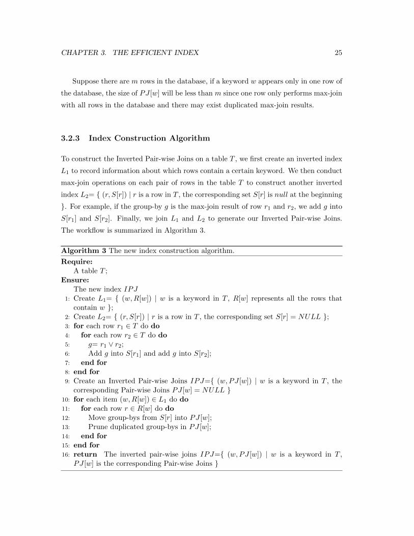
3.2.3 Index Construction Algorithm
To construct the Inverted Pair-wise Joins on a table T , we first create an inverted index
L1 to record information about which rows contain a certain keyword. We then conduct
max-join operations on each pair of rows in the table T to construct another inverted
index L2= (r, S[r]) | r is a row in T , the corresponding set S[r] is null at the beginning
. For example, if the group-by g is the max-join result of row r1 and r2, we add g into
S[r1] and S[r2]. Finally, we join L1 and L2 to generate our Inverted Pair-wise Joins.
The workflow is summarized in Algorithm 3.
Algorithm 3 The new index construction algorithm.
Require:A table T ;
Ensure:The new index IPJ
1: Create L1= (w,R[w]) | w is a keyword in T , R[w] represents all the rows thatcontain w ;
2: Create L2= (r, S[r]) | r is a row in T , the corresponding set S[r] = NULL ;3: for each row r1 ∈ T do do4: for each row r2 ∈ T do do5: g= r1 ∨ r2;6: Add g into S[r1] and add g into S[r2];7: end for8: end for9: Create an Inverted Pair-wise Joins IPJ= (w,PJ [w]) | w is a keyword in T , the
corresponding Pair-wise Joins PJ [w] = NULL 10: for each item (w,R[w]) ∈ L1 do do11: for each row r ∈ R[w] do do12: Move group-bys from S[r] into PJ [w];13: Prune duplicated group-bys in PJ [w];14: end for15: end for16: return The inverted pair-wise joins IPJ= (w,PJ [w]) | w is a keyword in T ,
PJ [w] is the corresponding Pair-wise Joins
3.2. THE NEW INDEX 26
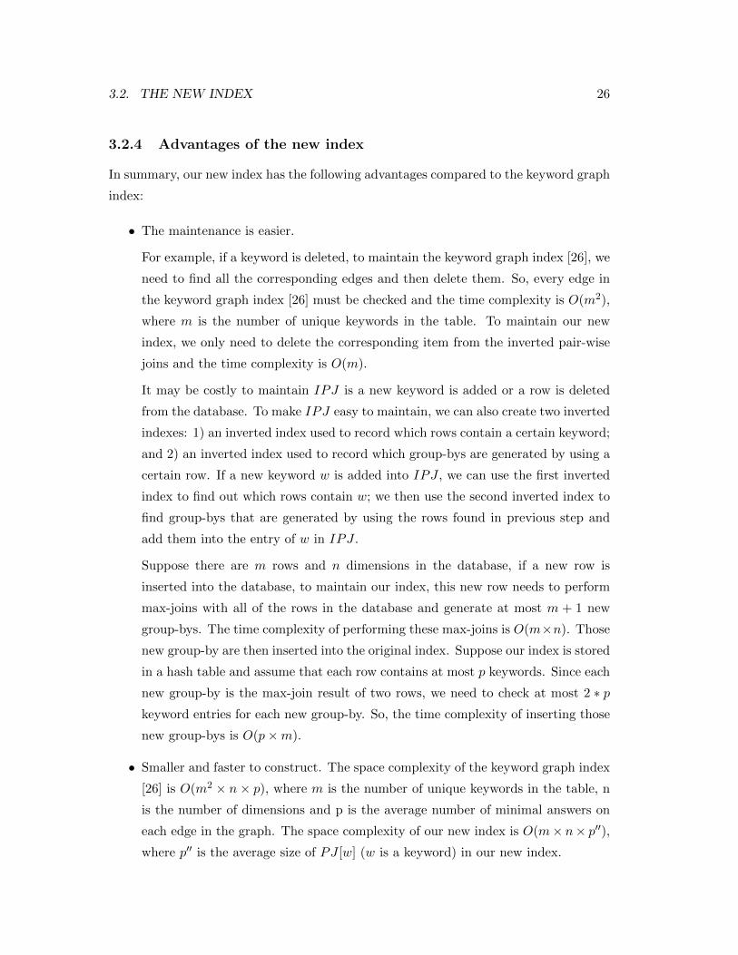
3.2.4 Advantages of the new index
In summary, our new index has the following advantages compared to the keyword graph
index:
• The maintenance is easier.
For example, if a keyword is deleted, to maintain the keyword graph index [26], we
need to find all the corresponding edges and then delete them. So, every edge in
the keyword graph index [26] must be checked and the time complexity is O(m2),
where m is the number of unique keywords in the table. To maintain our new
index, we only need to delete the corresponding item from the inverted pair-wise
joins and the time complexity is O(m).
It may be costly to maintain IPJ is a new keyword is added or a row is deleted
from the database. To make IPJ easy to maintain, we can also create two inverted
indexes: 1) an inverted index used to record which rows contain a certain keyword;
and 2) an inverted index used to record which group-bys are generated by using a
certain row. If a new keyword w is added into IPJ , we can use the first inverted
index to find out which rows contain w; we then use the second inverted index to
find group-bys that are generated by using the rows found in previous step and
add them into the entry of w in IPJ .
Suppose there are m rows and n dimensions in the database, if a new row is
inserted into the database, to maintain our index, this new row needs to perform
max-joins with all of the rows in the database and generate at most m + 1 new
group-bys. The time complexity of performing these max-joins is O(m×n). Those
new group-by are then inserted into the original index. Suppose our index is stored
in a hash table and assume that each row contains at most p keywords. Since each
new group-by is the max-join result of two rows, we need to check at most 2 ∗ pkeyword entries for each new group-by. So, the time complexity of inserting those
new group-bys is O(p×m).
• Smaller and faster to construct. The space complexity of the keyword graph index
[26] is O(m2 × n× p), where m is the number of unique keywords in the table, n
is the number of dimensions and p is the average number of minimal answers on
each edge in the graph. The space complexity of our new index is O(m× n× p′′),where p′′ is the average size of PJ [w] (w is a keyword) in our new index.
CHAPTER 3. THE EFFICIENT INDEX 27
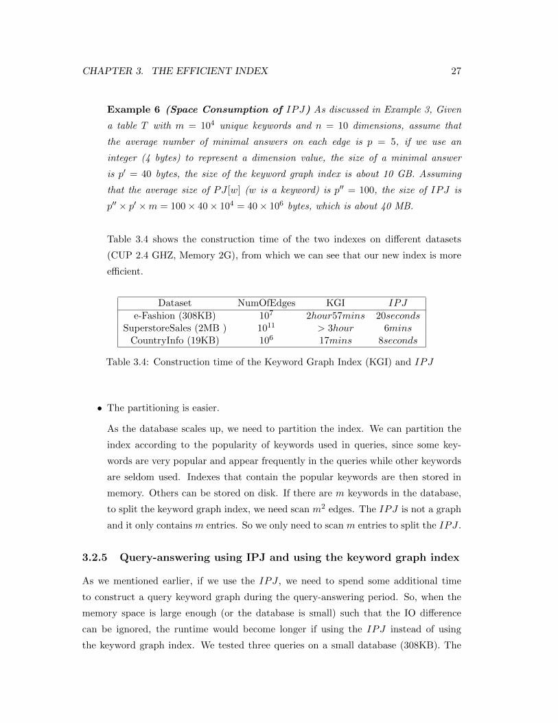
Example 6 (Space Consumption of IPJ) As discussed in Example 3, Given
a table T with m = 104 unique keywords and n = 10 dimensions, assume that
the average number of minimal answers on each edge is p = 5, if we use an
integer (4 bytes) to represent a dimension value, the size of a minimal answer
is p′ = 40 bytes, the size of the keyword graph index is about 10 GB. Assuming
that the average size of PJ [w] (w is a keyword) is p′′ = 100, the size of IPJ is
p′′ × p′ ×m = 100× 40× 104 = 40× 106 bytes, which is about 40 MB.
Table 3.4 shows the construction time of the two indexes on different datasets
(CUP 2.4 GHZ, Memory 2G), from which we can see that our new index is more
efficient.
Dataset NumOfEdges KGI IPJ
e-Fashion (308KB) 107 2hour57mins 20secondsSuperstoreSales (2MB ) 1011 > 3hour 6mins
CountryInfo (19KB) 106 17mins 8seconds
Table 3.4: Construction time of the Keyword Graph Index (KGI) and IPJ
• The partitioning is easier.
As the database scales up, we need to partition the index. We can partition the
index according to the popularity of keywords used in queries, since some key-
words are very popular and appear frequently in the queries while other keywords
are seldom used. Indexes that contain the popular keywords are then stored in
memory. Others can be stored on disk. If there are m keywords in the database,
to split the keyword graph index, we need scan m2 edges. The IPJ is not a graph
and it only contains m entries. So we only need to scan m entries to split the IPJ .
3.2.5 Query-answering using IPJ and using the keyword graph index
As we mentioned earlier, if we use the IPJ , we need to spend some additional time
to construct a query keyword graph during the query-answering period. So, when the
memory space is large enough (or the database is small) such that the IO difference
can be ignored, the runtime would become longer if using the IPJ instead of using
the keyword graph index. We tested three queries on a small database (308KB). The

3.2. THE NEW INDEX 28
memory size in the experiments is 1GB, which is large enough for storing all the data.
The results are shown in Table 3.5.
If the memory is not large enough or the database becomes larger, using the keyword
graph index would become less efficient because of the additional IO costs. We tested
three other queries on a larger database (2MB). The memory size is still 1GB. The
results are shown in Table 3.6. In summary, IPJ can help to improve the efficiency for
aggregate keyword search on large relational databases.
Dataset Query keywords KGI (msec) IPJ(msec)
e-Fashion Jackets Leather Sweaters 2001 599 751e-Fashion Jackets Leather Sweaters 591 656e-Fashion 2001 2002 2003 Jackets 1797 2668
Table 3.5: Runtime of query-answering on the e-Fashion dataset using Keyword GraphIndex (KGI) and using IPJ
Dataset Query keywords KGI (msec) IPJ(msec)
SuperstoreSales Paper Envelopes Tables 45855 32468SuperstoreSales Roy Matt Collins 13402 1810SuperstoreSales Tracy Truck Box 317118 308757
Table 3.6: Runtime of query-answering on the SuperstoreSales dataset using keywordgraph index and using IPJ

Chapter 4
The Top-k Algorithm
Zhou and Pei [26] return all the minimal answers (unranked) for an aggregate keyword
query. As the relational database grows larger, there could be many minimal answers
for an individual query. In such a case, finding all the minimal answers without ranking
may overwhelm users.
We propose a general ranking model and an efficient ranking algorithm. Our top-
k query answering method provides users with top-k answers in a short time than
computing all minimal answers. It works in two steps, the bounding step and the
pruning step, to generate top-k results. The two steps can help to prune unnecessary
max-join operations and save the query processing time.
In this section, we present the scoring function and top-k query answering method.
4.1 Scoring Function
We define three scoring functions on a group-by: the density score, the dedication score
and the structure degree. The overall score of a group-by is a linear combination of
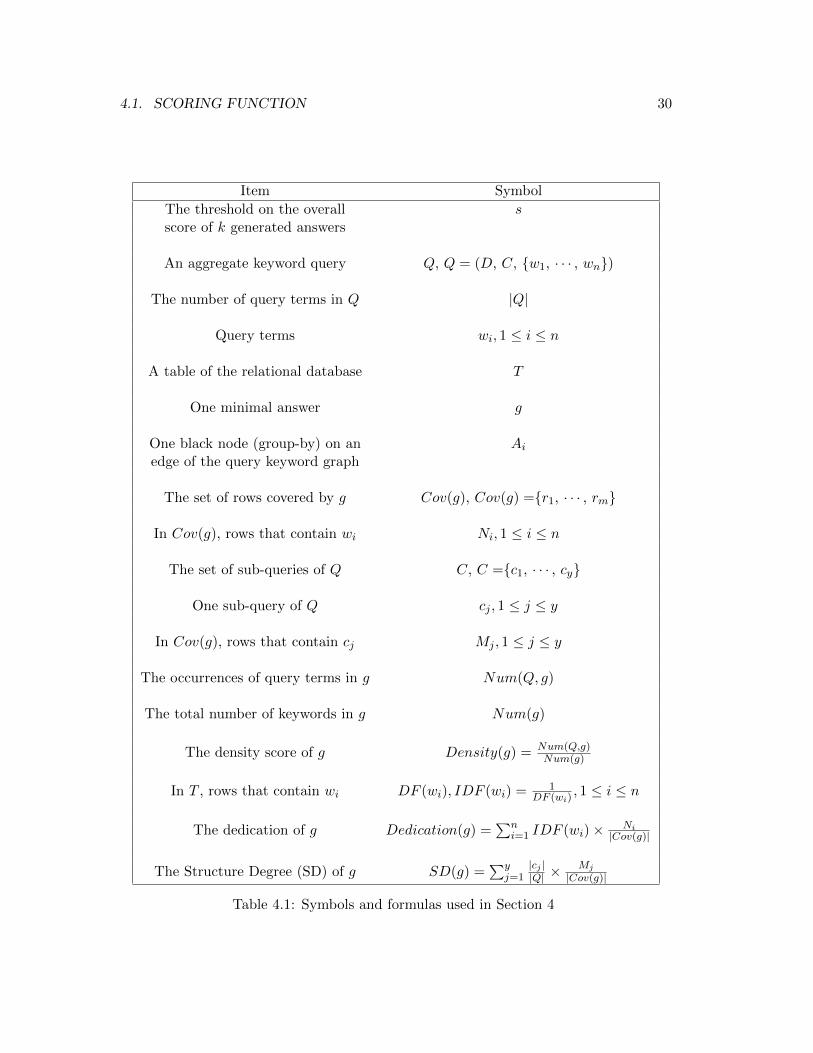
these three scores. Table 4.1 presents the symbols and formulas used in this section.
4.1.1 Density Score
We use a density score to measure whether the query keywords appear frequently in the
minimal answers. If a group-by has a high density score, it means that query keywords
appear frequently in this group-by, and thus this group-by should be ranked high in the
search engine.
29
4.1. SCORING FUNCTION 30
Item Symbol
The threshold on the overall sscore of k generated answers
An aggregate keyword query Q, Q = (D, C, w1, · · · , wn)
The number of query terms in Q |Q|
Query terms wi, 1 ≤ i ≤ n
A table of the relational database T
One minimal answer g
One black node (group-by) on an Ai
edge of the query keyword graph
The set of rows covered by g Cov(g), Cov(g) =r1, · · · , rm
In Cov(g), rows that contain wi Ni, 1 ≤ i ≤ n
The set of sub-queries of Q C, C =c1, · · · , cy
One sub-query of Q cj , 1 ≤ j ≤ y
In Cov(g), rows that contain cj Mj , 1 ≤ j ≤ y
The occurrences of query terms in g Num(Q, g)
The total number of keywords in g Num(g)
The density score of g Density(g) = Num(Q,g)Num(g)
In T , rows that contain wi DF (wi), IDF (wi) = 1DF (wi)
, 1 ≤ i ≤ n
The dedication of g Dedication(g) =∑n
i=1 IDF (wi)× Ni|Cov(g)|
The Structure Degree (SD) of g SD(g) =∑y
j=1|cj ||Q| ×
Mj
|Cov(g)|
Table 4.1: Symbols and formulas used in Section 4
CHAPTER 4. THE TOP-K ALGORITHM 31
The feature of term frequency is often used in IR technologies [21, 23]. Since each
group-by covers a set of rows in the table T , we can treat these covered rows as a
document and similarly consider the query term frequency in these covered rows.
Definition 8 (Density Score) Given an aggregate query Q, the density score of a
group-by g is defined as
Density(g) = Density(Cov(g)) =Num(Q, g)
Num(g)(4.1)
where Num(Q, g) is the total number of occurrences of query terms in the group-by
g, Num(g) represents the total number of keywords in g, and Cov(g) represents rows
covered by g.
We calculate the density score of a group-by g by using information in its covered
rows (Cov(g)). Therefore, in this thesis, Density(g) and Density(Cov(g)) are the same.
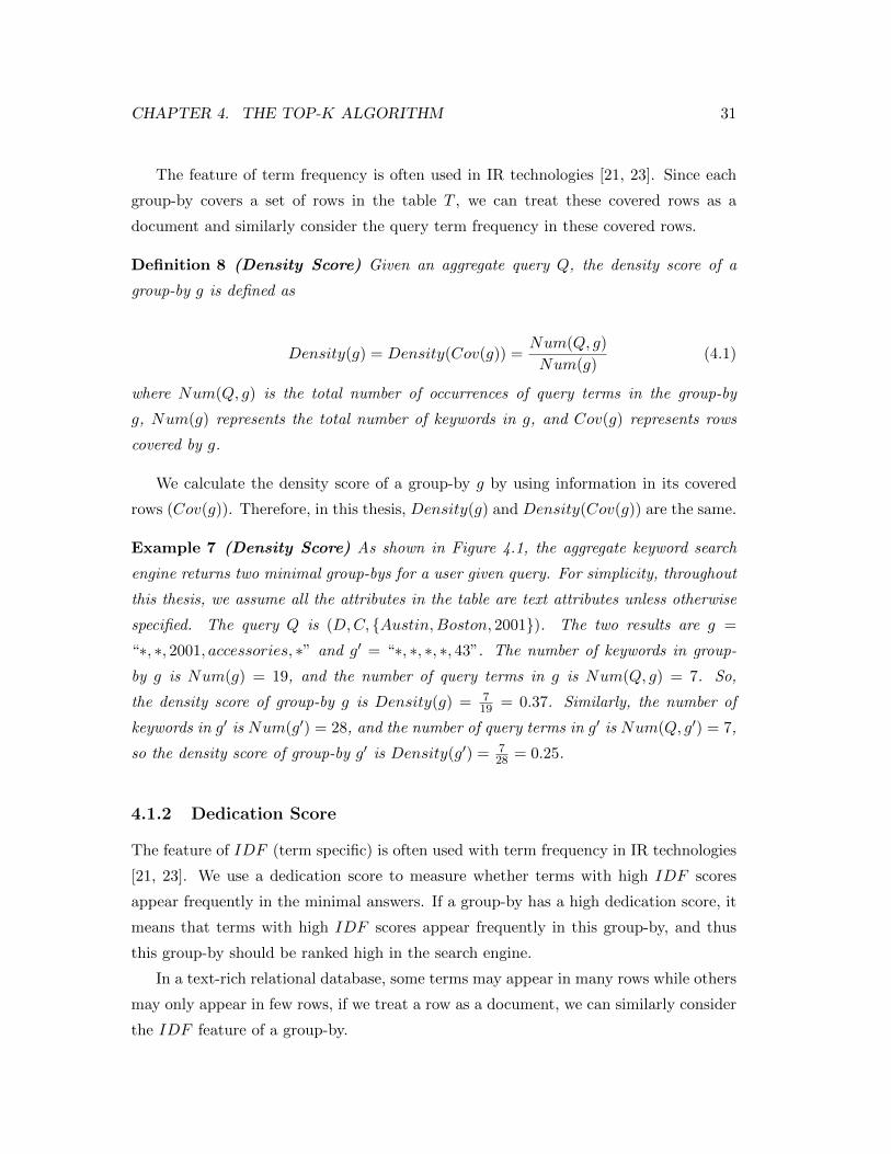
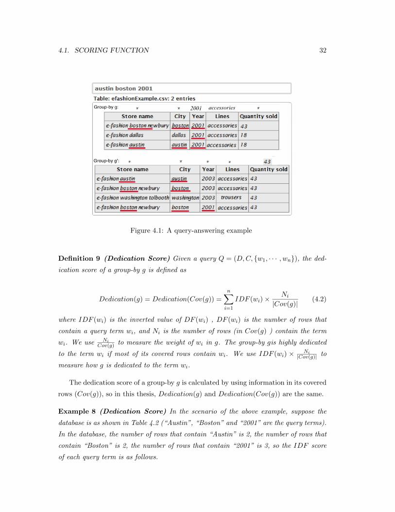
Example 7 (Density Score) As shown in Figure 4.1, the aggregate keyword search
engine returns two minimal group-bys for a user given query. For simplicity, throughout
this thesis, we assume all the attributes in the table are text attributes unless otherwise
specified. The query Q is (D,C, Austin,Boston, 2001). The two results are g =
“∗, ∗, 2001, accessories, ∗” and g′ = “∗, ∗, ∗, ∗, 43”. The number of keywords in group-
by g is Num(g) = 19, and the number of query terms in g is Num(Q, g) = 7. So,
the density score of group-by g is Density(g) = 719 = 0.37. Similarly, the number of
keywords in g′ is Num(g′) = 28, and the number of query terms in g′ is Num(Q, g′) = 7,
so the density score of group-by g′ is Density(g′) = 728 = 0.25.
4.1.2 Dedication Score
The feature of IDF (term specific) is often used with term frequency in IR technologies
[21, 23]. We use a dedication score to measure whether terms with high IDF scores
appear frequently in the minimal answers. If a group-by has a high dedication score, it
means that terms with high IDF scores appear frequently in this group-by, and thus
this group-by should be ranked high in the search engine.
In a text-rich relational database, some terms may appear in many rows while others
may only appear in few rows, if we treat a row as a document, we can similarly consider
the IDF feature of a group-by.
4.1. SCORING FUNCTION 32
Figure 4.1: A query-answering example
Definition 9 (Dedication Score) Given a query Q = (D,C, w1, · · · , wn), the ded-
ication score of a group-by g is defined as
Dedication(g) = Dedication(Cov(g)) =n∑
i=1
IDF (wi)×Ni
|Cov(g)|(4.2)
where IDF (wi) is the inverted value of DF (wi) , DF (wi) is the number of rows that
contain a query term wi, and Ni is the number of rows (in Cov(g) ) contain the term
wi. We use NiCov(g) to measure the weight of wi in g. The group-by gis highly dedicated
to the term wi if most of its covered rows contain wi. We use IDF (wi) × Ni|Cov(g)| to
measure how g is dedicated to the term wi.
The dedication score of a group-by g is calculated by using information in its covered
rows (Cov(g)), so in this thesis, Dedication(g) and Dedication(Cov(g)) are the same.
Example 8 (Dedication Score) In the scenario of the above example, suppose the
database is as shown in Table 4.2 (“Austin”, “Boston” and “2001” are the query terms).
In the database, the number of rows that contain “Austin” is 2, the number of rows that
contain “Boston” is 2, the number of rows that contain “2001” is 3, so the IDF score
of each query term is as follows.

CHAPTER 4. THE TOP-K ALGORITHM 33
IDF (“Austin”) = 12 = 0.5
IDF (“Boston”) = 12 = 0.5
IDF (“2001”) = 13 = 0.33
In Figure 4.1, the number of rows covered by group-by g = “∗, ∗, 2001, accessories, ∗”is |Cov(g)| = 3, the number of rows in Cov(g) that contain “Austin” is N1 = 1, the
number of rows in Cov(g) that contain “Boston” is N2 = 1 and the number of rows
in Cov(g) that contain “2001” is N3 = 3. So, the dedication score of group-by g is
Dedication(g) = 0.5 × 13 + 0.5 × 1
3 + 0.33 × 33 = 0.66. Similarly, the number of rows
covered by group-by g′ = “∗, ∗, ∗, ∗, 43” is |Cov(g′)| = 4, the number of rows in Cov(g′)
that contain “Austin” is N1 = 1, the number of rows in Cov(g′) that contain “Boston”
is N2 = 2 and the number of rows in Cov(g′) that contain “2001” is N3 = 1. So, the
dedication score of group-by g′ is Dedication(g′) = 0.5× 14 + 0.5× 2
4 + 0.33× 14 = 0.46.
StoreName City Year Lines QuantitySold
e-Fashion Austin Austin 2003 accsesories 43e-Fashion Boston Newbury Boston 2003 accessories 43
e-Fashion Washington Tolbooth Washington 2003 trousers 43e-Fashion Boston Newbury Boston 2001 accessories 43
e-Fashion Dallas Dallas 2001 accessories 18e-Fashion Washington Tolbooth Washington 2002 trousers 18e-Fashion Washington Tolbooth Washington 2003 dresses 18
e-Fashion Austin Austin 2001 accessories 18
Table 4.2: Query Keywords in the e-Fashion Database
4.1.3 Structure Degree
If a keyword query Q = (D,C, w1, · · · , wn), there exists 2n sub-queries (including
the empty sub-query). Each row in the database matches one of these sub-queries
(if a row has no query keyword inside, it matches the empty sub-query). Different
sub-queries may have different importance and we assume that longer sub-queries are
more important than shorter ones. A group-by is good if its covered rows match many
important sub-queries.
We use a structure degree to measure whether important sub-queries (structures)
appear frequently in the minimal answers. If a group-by has a high structure degree, it

4.1. SCORING FUNCTION 34
means that important sub-queries (structures) appear frequently in this group-by, and
thus this group-by should be ranked high in the search engine.
Definition 10 (Structure Degree) Given a query Q, the sub-queries of Q are c1,
· · · , cy, the structure degree of a group-by g is defined as
StructureDegree(g) = StructureDegree(Cov(g)) =
y∑j=1
|cj ||Q|× Mj
|Cov(g)|(4.3)
where Mj is the number of rows in Cov(g) that contain the sub-query cj.
Since we assume that longer sub-queries are more important than shorter ones ,
we can use|cj ||Q| to measure the importance of a sub-query cj . Also, we use
Mj
|Cov(g)| to
measure the weight of cj in the group-by g, thus the score of cj in group-by g can be
measured by using|cj ||Q| ×
Mj
|Cov(g)| .
The structure degree of a group-by g is calculated by using information in its covered
rows (Cov(g)), so in this thesis, StructureDegree(g) and StructureDegree(Cov(g)) are
the same.
Example 9 (Structure Degree) In the scenario of the above two examples, the search
engine returns two group-bys ( g and g′ ) for the query (D,C, Austin,Boston, 2001).For group-by g = “∗, ∗, 2001, accessories, ∗”, its covered rows match the following sub-
queries:
(D,C, Boston, 2001), (D,C, Austin, 2001), (D,C, 2001)For group-by g′ = “∗, ∗, ∗, ∗, 43”, its covered rows match the following sub-queries:
(D,C, Boston, 2001), (D,C, Austin), (D,C, Boston)In Figure 4.1, the number of rows covered by group-by g is |Cov(g)| = 3, the
number of rows in Cov(g) that match (D,C, Boston, 2001) is M1 = 1, the num-
ber of rows in Cov(g) that match (D,C, Austin, 2001) is M2 = 1 and the num-
ber of rows in Cov(g) that match (D,C, 2001) is M3 = 1. So, the structure de-
gree of group-by g is StructureDegree(g) = 23 ×
13 + 1
3 ×13 + 2
3 ×13 = 0.56. Sim-
ilarly, the number of rows covered by group-by g′ is |Cov(g′)| = 4, the number of
rows in Cov(g′) that match (D,C, Boston, 2001) is M1 = 1, the number of rows
in Cov(g′) that match (D,C, Austin) is M2 = 1 and the number of rows in Cov(g′)
that match (D,C, Boston) is M3 = 1. So, the structure degree of group-by g′ is
StructureDegree(g′) = 13 ×
14 + 1
3 ×14 + 2
3 ×14 = 0.33.
CHAPTER 4. THE TOP-K ALGORITHM 35
4.1.4 The Overall Scoring Function
In this thesis, assuming that the max-join result of group-by g1 and group-by g2 is g,
the scores of group-by g can be calculated by using information in Cov(g1)⋃Cov(g2).
The overall score of group-by g is the linear combination of its density score, dedication
score and structure degree, which is shown in the following equation.
Score(g)
= Score(Cov(g1)⋃Cov(g2))
= e1 ×Density(g) + e2 ×Dedication(g) + (1− e1 − e2)× StructureDegree(g)
(4.4)
where e1, e2 are two coefficients, 0 ≤ e1, e2 ≤ 1.
4.2 Query Processing
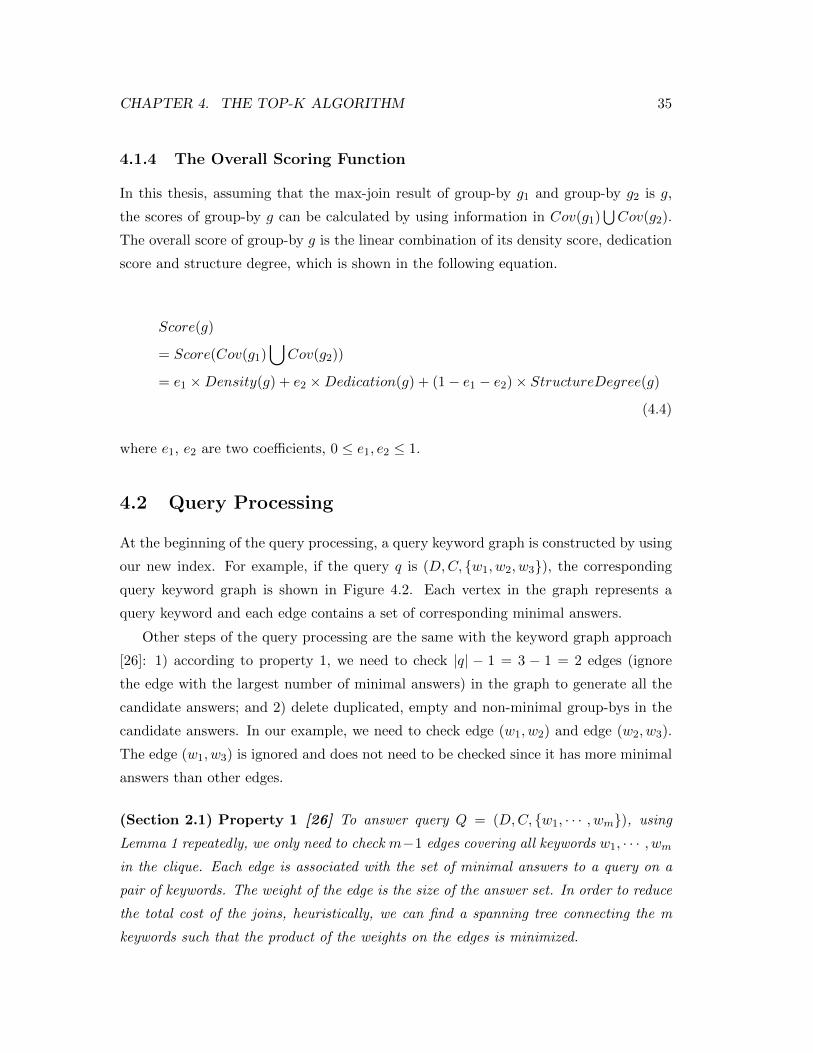
At the beginning of the query processing, a query keyword graph is constructed by using
our new index. For example, if the query q is (D,C, w1, w2, w3), the corresponding
query keyword graph is shown in Figure 4.2. Each vertex in the graph represents a
query keyword and each edge contains a set of corresponding minimal answers.
Other steps of the query processing are the same with the keyword graph approach
[26]: 1) according to property 1, we need to check |q| − 1 = 3 − 1 = 2 edges (ignore
the edge with the largest number of minimal answers) in the graph to generate all the
candidate answers; and 2) delete duplicated, empty and non-minimal group-bys in the
candidate answers. In our example, we need to check edge (w1, w2) and edge (w2, w3).
The edge (w1, w3) is ignored and does not need to be checked since it has more minimal
answers than other edges.
(Section 2.1) Property 1 [26] To answer query Q = (D,C, w1, · · · , wm), using
Lemma 1 repeatedly, we only need to check m−1 edges covering all keywords w1, · · · , wm
in the clique. Each edge is associated with the set of minimal answers to a query on a
pair of keywords. The weight of the edge is the size of the answer set. In order to reduce
the total cost of the joins, heuristically, we can find a spanning tree connecting the m
keywords such that the product of the weights on the edges is minimized.

4.2. QUERY PROCESSING 36
Figure 4.2: An example of Query Keyword Graph in Chapter 4
(Section 2.1) Lemma 1 (Max-join on answers) [26] If t is a minimal answer to
aggregate keyword query Q = (D,C, w1, · · · , wm), then there exists minimal answers
t1 and t2 to queries (D,C, w1, w2) and (D,C, we, · · · , wm), respectively, such that
t = t1 ∨ t2.
Definition 11 (node, back node, line and white node) In the query keyword graph,
each edge is associated with a set of minimal answers. We use a node to represent
a minimal answer of the corresponding edge, as shown in Figure 4.2. All nodes are
black nodes at the beginning. As shown in Figure 4.3, each line represents a max-join
operation on two black nodes. The max-join result is a candidate answer. We need to
perform 12 max-join operations in order to generate all the candidate answers. Our top-
k method detects some black nodes as white nodes (Figure 4.4), such that if max-joins
are all on white nodes, the corresponding max-join results are not top-k answers.
We have to do many max-join operations if generating all minimal answers. Since
we only need top-k answers, some unnecessary max-join operations can be pruned.
We develop a two-step (the bounding step and the pruning step) pruning method to
prune unnecessary max-join operations. In Figure 4.3, each node represents a minimal
answer in the corresponding edge. All these nodes are black at the beginning. To
prune unnecessary joins, the bounding step detects some black nodes as white nodes
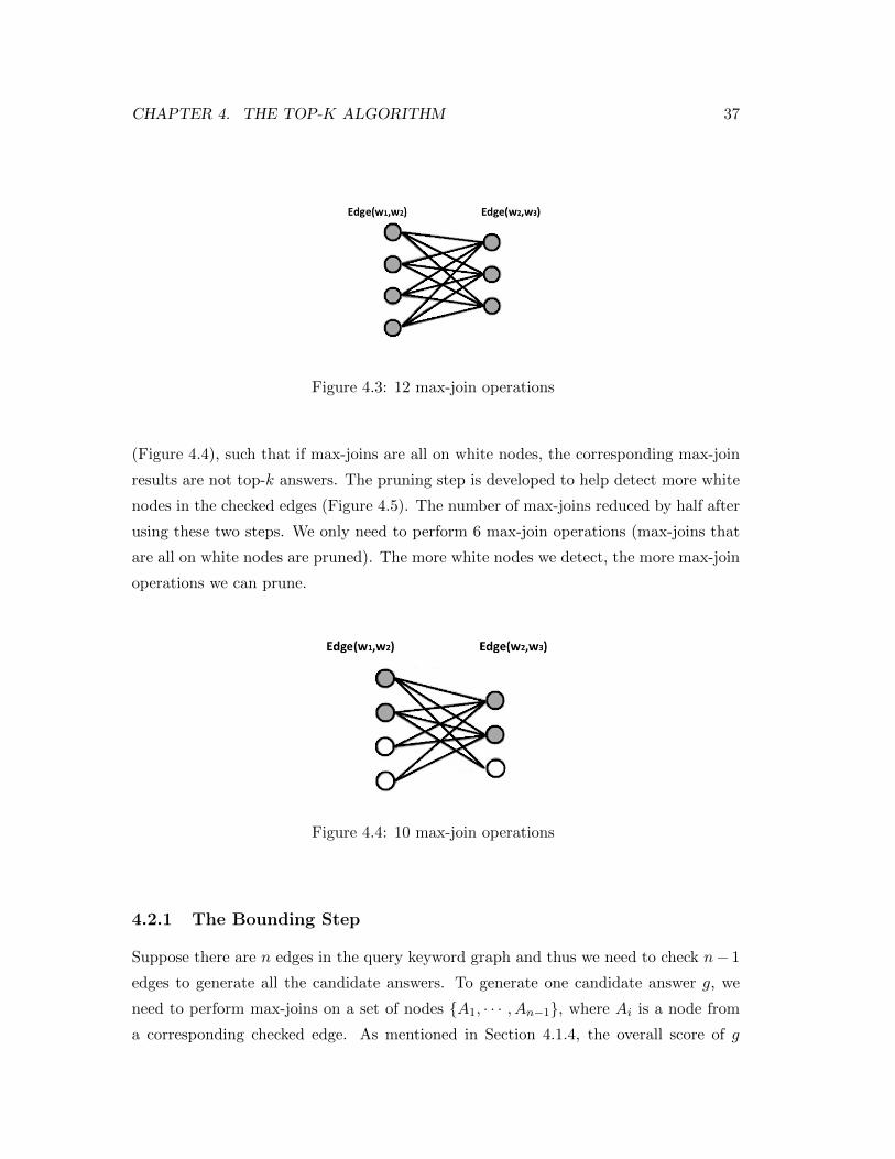
CHAPTER 4. THE TOP-K ALGORITHM 37
Figure 4.3: 12 max-join operations
(Figure 4.4), such that if max-joins are all on white nodes, the corresponding max-join
results are not top-k answers. The pruning step is developed to help detect more white
nodes in the checked edges (Figure 4.5). The number of max-joins reduced by half after
using these two steps. We only need to perform 6 max-join operations (max-joins that
are all on white nodes are pruned). The more white nodes we detect, the more max-join
operations we can prune.
Figure 4.4: 10 max-join operations
4.2.1 The Bounding Step
Suppose there are n edges in the query keyword graph and thus we need to check n− 1
edges to generate all the candidate answers. To generate one candidate answer g, we
need to perform max-joins on a set of nodes A1, · · · , An−1, where Ai is a node from
a corresponding checked edge. As mentioned in Section 4.1.4, the overall score of g
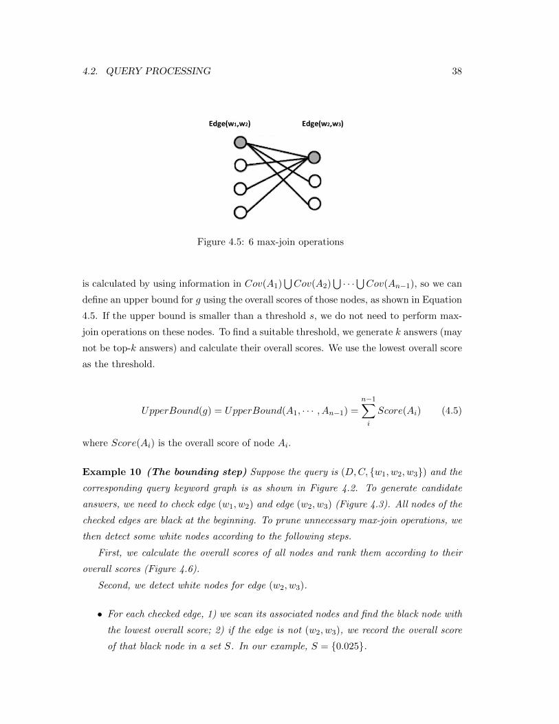
4.2. QUERY PROCESSING 38
Figure 4.5: 6 max-join operations
is calculated by using information in Cov(A1)⋃Cov(A2)
⋃· · ·⋃Cov(An−1), so we can
define an upper bound for g using the overall scores of those nodes, as shown in Equation
4.5. If the upper bound is smaller than a threshold s, we do not need to perform max-
join operations on these nodes. To find a suitable threshold, we generate k answers (may
not be top-k answers) and calculate their overall scores. We use the lowest overall score
as the threshold.
UpperBound(g) = UpperBound(A1, · · · , An−1) =
n−1∑i
Score(Ai) (4.5)
where Score(Ai) is the overall score of node Ai.
Example 10 (The bounding step) Suppose the query is (D,C, w1, w2, w3) and the
corresponding query keyword graph is as shown in Figure 4.2. To generate candidate
answers, we need to check edge (w1, w2) and edge (w2, w3) (Figure 4.3). All nodes of the
checked edges are black at the beginning. To prune unnecessary max-join operations, we
then detect some white nodes according to the following steps.
First, we calculate the overall scores of all nodes and rank them according to their
overall scores (Figure 4.6).
Second, we detect white nodes for edge (w2, w3).
• For each checked edge, 1) we scan its associated nodes and find the black node with
the lowest overall score; 2) if the edge is not (w2, w3), we record the overall score
of that black node in a set S. In our example, S = 0.025.
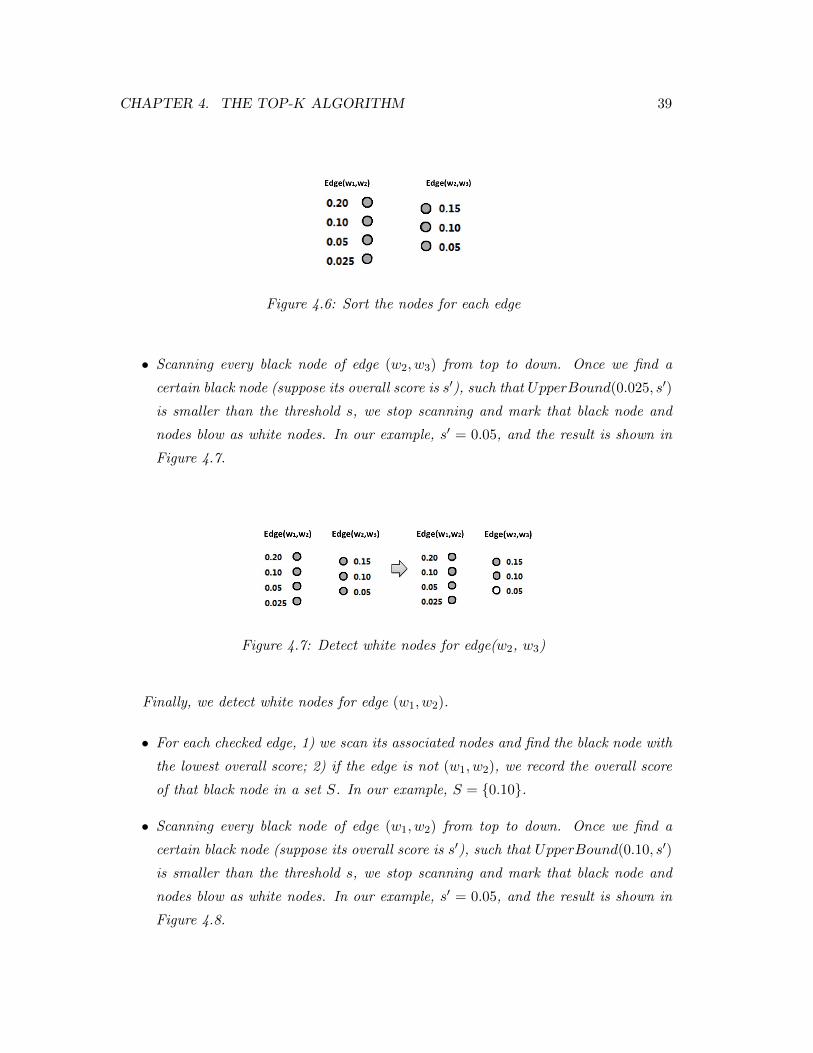
CHAPTER 4. THE TOP-K ALGORITHM 39
Figure 4.6: Sort the nodes for each edge
• Scanning every black node of edge (w2, w3) from top to down. Once we find a
certain black node (suppose its overall score is s′), such that UpperBound(0.025, s′)
is smaller than the threshold s, we stop scanning and mark that black node and
nodes blow as white nodes. In our example, s′ = 0.05, and the result is shown in
Figure 4.7.
Figure 4.7: Detect white nodes for edge(w2, w3)
Finally, we detect white nodes for edge (w1, w2).
• For each checked edge, 1) we scan its associated nodes and find the black node with
the lowest overall score; 2) if the edge is not (w1, w2), we record the overall score
of that black node in a set S. In our example, S = 0.10.
• Scanning every black node of edge (w1, w2) from top to down. Once we find a
certain black node (suppose its overall score is s′), such that UpperBound(0.10, s′)
is smaller than the threshold s, we stop scanning and mark that black node and
nodes blow as white nodes. In our example, s′ = 0.05, and the result is shown in
Figure 4.8.
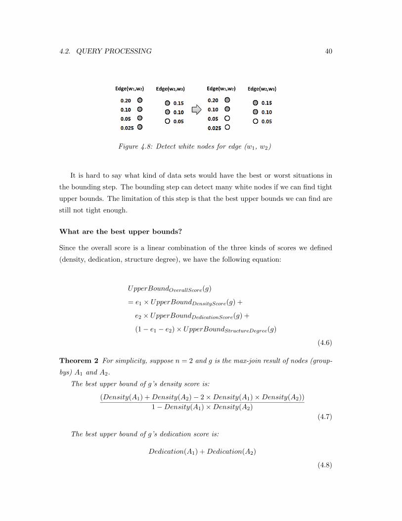
4.2. QUERY PROCESSING 40
Figure 4.8: Detect white nodes for edge (w1, w2)
It is hard to say what kind of data sets would have the best or worst situations in
the bounding step. The bounding step can detect many white nodes if we can find tight
upper bounds. The limitation of this step is that the best upper bounds we can find are
still not tight enough.
What are the best upper bounds?
Since the overall score is a linear combination of the three kinds of scores we defined
(density, dedication, structure degree), we have the following equation:
UpperBoundOverallScore(g)
= e1 × UpperBoundDensityScore(g) +
e2 × UpperBoundDedicationScore(g) +
(1− e1 − e2)× UpperBoundStructureDegree(g)
(4.6)
Theorem 2 For simplicity, suppose n = 2 and g is the max-join result of nodes (group-
bys) A1 and A2.
The best upper bound of g’s density score is:
(Density(A1) +Density(A2)− 2×Density(A1)×Density(A2))
1−Density(A1)×Density(A2)
(4.7)
The best upper bound of g’s dedication score is:
Dedication(A1) +Dedication(A2)
(4.8)
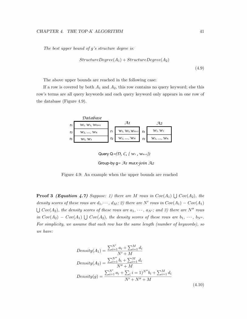
CHAPTER 4. THE TOP-K ALGORITHM 41
The best upper bound of g’s structure degree is:
StructureDegree(A1) + StructureDegree(A2)
(4.9)
The above upper bounds are reached in the following case:
If a row is covered by both A1 and A2, this row contains no query keyword; else this
row’s terms are all query keywords and each query keyword only appears in one row of
the database (Figure 4.9).
Figure 4.9: An example when the upper bounds are reached
Proof 3 (Equation 4.7) Suppose: 1) there are M rows in Cov(A1)⋃Cov(A2), the
density scores of these rows are d1,· · · , dM ; 2) there are N ′ rows in Cov(A1) − Cov(A1)⋃Cov(A2), the density scores of these rows are a1, · · · , aN ′; and 3) there are N ′′ rows
in Cov(A2) − Cov(A1)⋃Cov(A2), the density scores of these rows are b1, · · · , bN ′′.
For simplicity, we assume that each row has the same length (number of keywords), so
we have:
Density(A1) =
∑N ′
i=1 ai +∑M
i=1 diN ′ +M
Density(A2) =
∑N ′′
i=1 bi +∑M
i=1 diN ′′ +M
Density(g) =
∑N ′
i=1 ai +∑
( i = 1)N′′bi +
∑Mi=1 di
N ′ +N ′′ +M(4.10)
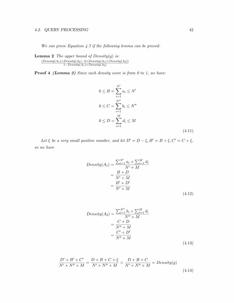
4.2. QUERY PROCESSING 42
We can prove Equation 4.7 if the following lemma can be proved:
Lemma 2 The upper bound of Density(g) is:(Density(A1)+Density(A2)−2×Density(A1)×Density(A2))
1−Density(A1)×Density(A2)
Proof 4 (Lemma 2) Since each density score is from 0 to 1, we have:
0 ≤ B =N ′∑i=1
ai ≤ N ′
0 ≤ C =
N ′′∑i=1
bi ≤ N ′′
0 ≤ D =M∑i=1
di ≤M
(4.11)
Let ξ be a very small positive number, and let D′ = D − ξ,B′ = B + ξ, C ′ = C + ξ,
so we have
Density(A1) =
∑N ′
i=1 ai +∑M
i=1 diN ′ +M
=B +D
N ′ +M
=B′ +D′
N ′ +M(4.12)
Density(A2) =
∑N ′′
i=1 bi +∑M
i=1 diN ′′ +M
=C +D
N ′′ +M
=C ′ +D′
N ′′ +M(4.13)
D′ +B′ + C ′
N ′ +N ′′ +M=D +B + C + ξ
N ′ +N ′′ +M>
D +B + C
N ′ +N ′′ +M= Density(g)
(4.14)
CHAPTER 4. THE TOP-K ALGORITHM 43
If D becomes smaller (or B and C become larger), Density(g) would become larger.
So, if the upper bound of Density(g) is reached, D must be 0, which means rows covered
by both A1 and A2 contain no query keywords.
Since D is 0, we have:
Density(g) =B + C
N ′ +N ′′ +M
Density(A1) =B
N ′ +M
Density(A2) =C
N ′′ +M(4.15)
Let M ′ = M + ξ,N ′1 = N ′ − ξ,N ′′1 = N ′′ − ξ, so we have:
B + C
N ′1 +N ′′1 +M ′=
B + C
N ′ +N ′′ +M − ξ>
B + C
N ′ +N ′′ +M= Density(g)
(4.16)
0 ≤ B =N ′∑i=1
ai ≤ N ′
0 ≤ C =N ′′∑i=1
bi ≤ N ′′
(4.17)
If N ′ and N ′′ become smaller(or M becomes larger), Density(g) would become larger.
So, if the upper bound of Density(g) is reached, N ′ must be B and N ′′ must be C, which
means a1 = · · · = aN ′ = 1 and b1 = · · · = bN ′′ = 1.
So, the upper bound of Density(g) is reached if D = 0, B = N ′ and C = N ′′. In
such a case, the upper bound of Density(g) is:
(Density(A1) +Density(A2)− 2×Density(A1)×Density(A2))
1−Density(A1)×Density(A2)
(4.18)
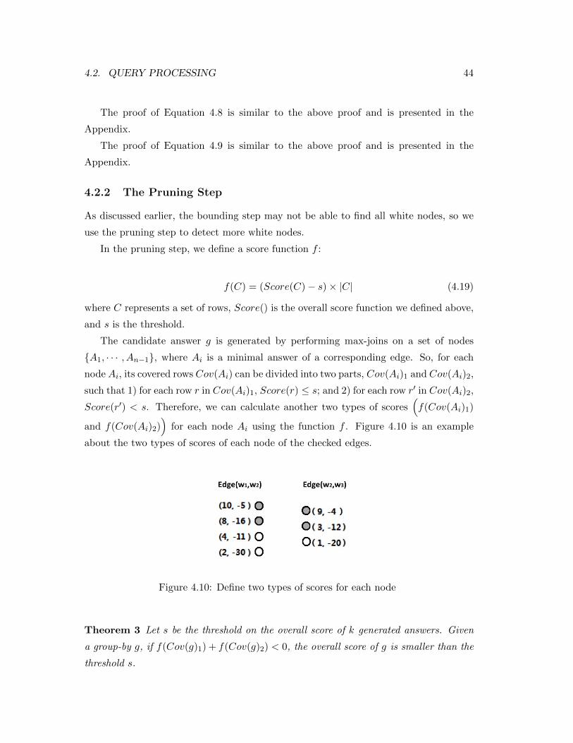
4.2. QUERY PROCESSING 44
The proof of Equation 4.8 is similar to the above proof and is presented in the
Appendix.
The proof of Equation 4.9 is similar to the above proof and is presented in the
Appendix.
4.2.2 The Pruning Step
As discussed earlier, the bounding step may not be able to find all white nodes, so we
use the pruning step to detect more white nodes.
In the pruning step, we define a score function f :
f(C) = (Score(C)− s)× |C| (4.19)
where C represents a set of rows, Score() is the overall score function we defined above,
and s is the threshold.
The candidate answer g is generated by performing max-joins on a set of nodes
A1, · · · , An−1, where Ai is a minimal answer of a corresponding edge. So, for each
node Ai, its covered rows Cov(Ai) can be divided into two parts, Cov(Ai)1 and Cov(Ai)2,
such that 1) for each row r in Cov(Ai)1, Score(r) ≤ s; and 2) for each row r′ in Cov(Ai)2,
Score(r′) < s. Therefore, we can calculate another two types of scores(f(Cov(Ai)1)
and f(Cov(Ai)2))
for each node Ai using the function f . Figure 4.10 is an example
about the two types of scores of each node of the checked edges.
Figure 4.10: Define two types of scores for each node
Theorem 3 Let s be the threshold on the overall score of k generated answers. Given
a group-by g, if f(Cov(g)1) + f(Cov(g)2) < 0, the overall score of g is smaller than the
threshold s.
CHAPTER 4. THE TOP-K ALGORITHM 45
Corollary 1 Let s be the threshold on the overall score of k generated answers. Suppose
the candidate answer g is generated by performing max-joins on a set of nodes (minimal
answers) A1, · · · , An−1, where Ai is a minimal answer of a corresponding checked
edge in the query keyword graph. If the following inequality is satisfied, the overall score
of g is smaller than the threshold s.
n−1∑i=1
f(Cov(Ai)1) + minf(Cov(A1)2), · · · , f(Cov(An−1)2) < 0
Proof 5 (Theorem 3) We need to prove that given a group-by g, if f(Cov(g)1) +
f(Cov(g)2) < 0, the overall score of g is smaller than the threshold s.
Proof:
According to the definition of function f , we have:
f(Cov(g)1) = (Score(Cov(g)1)− s)× |Cov(g)1|
f(Cov(g)2) = (Score(Cov(g)2)− s)× |Cov(g)2|
(4.20)
We already know that f(Cov(g)1) + f(Cov(g)2) < 0, so we have:
0 >
f(Cov(g)1) + f(Cov(g)2)
= (Score(Cov(g)1)− s)× |Cov(g)1)|+ (Score(Cov(g)2)− s)× |Cov(g)2|
= Score(Cov(g)1)× |Cov(g)1|+ Score(Cov(g)2)× |Cov(g)2|
−s× (|Cov(g)1|+ |Cov(g)2|)
= Score(Cov(g)1)× |Cov(g)1|+ Score(Cov(g)2)× |Cov(g)2| − s× |Cov(g)|
(4.21)
s× |Cov(g)| > Score(Cov(g)1)× |Cov(g)1|+ Score(Cov(g)2)× |Cov(g)2|
s >Score(Cov(g)1)× |Cov(g)1|+ Score(Cov(g)2)× |Cov(g)2|
|Cov(g)|(4.22)
So we only need to prove the following equation:
4.2. QUERY PROCESSING 46
Score(Cov(g)) =Score(Cov(g)1)× |Cov(g)1|+ Score(Cov(g)2)× |Cov(g)2|
|Cov(g)|(4.23)
For simplicity, we assume that each row has the same length l (number of keywords),
and we have:
Density(Cov(g))
=Density(Cov(g)1)×Num(Cov(g)1) +Density(Cov(g)2)×Num(Cov(g)2)
Num(Cov(g))
=Density(Cov(g)1)× |Cov(g)1| × l +Density(Cov(g)2)× |Cov(g)2| × l
|Cov(g)| × l
=Density(Cov(g)1)× |Cov(g)1|+Density(Cov(g)2)× |Cov(g)2|
|Cov(g)|(4.24)
Dedication(Cov(g))
=n∑
i=1
IDF (wi)×Ni
|Cov(g)|
=
∑ni=1 IDF (wi)×Ni
|Cov(g)|
=
∑ni=1 IDF (wi)× (N ′i +N ′′i )
|Cov(g)|
=
∑ni=1 IDF (wi)×N ′i + sumn
i=1IDF (wi)×N ′′i|Cov(g)|
=|Cov(g)1| ×
∑ni=1 IDF (wi)×
N ′i
|Cov(g)1| + |Cov(g)2| × sumni=1IDF (wi)×
N ′′i
|Cov(g)2|
|Cov(g)|
=|Cov(g)1| ×Dedication(Cov(g)1) + |Cov(g)2| ×Dedication(Cov(g)2)
|Cov(g)|(4.25)
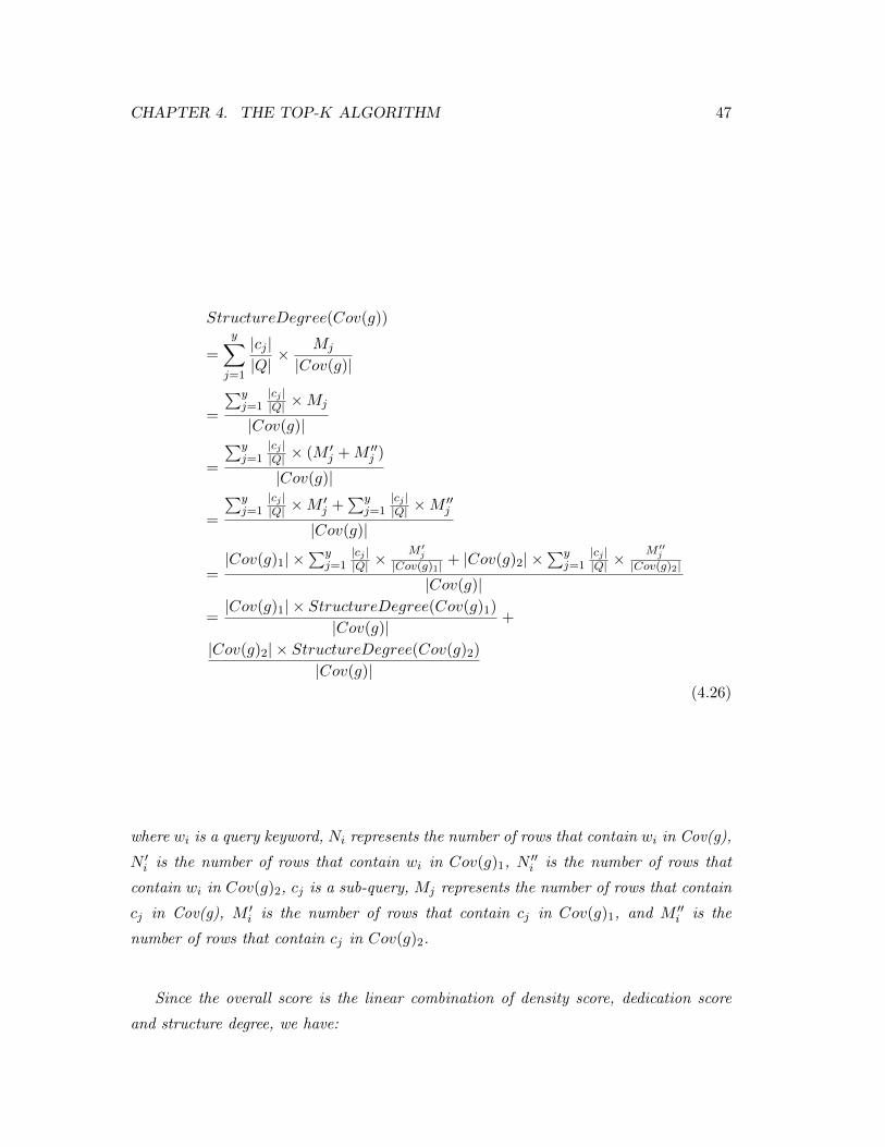
CHAPTER 4. THE TOP-K ALGORITHM 47
StructureDegree(Cov(g))
=
y∑j=1
|cj ||Q|× Mj
|Cov(g)|
=
∑yj=1
|cj ||Q| ×Mj
|Cov(g)|
=
∑yj=1
|cj ||Q| × (M ′j +M ′′j )
|Cov(g)|
=
∑yj=1
|cj ||Q| ×M
′j +
∑yj=1
|cj ||Q| ×M
′′j
|Cov(g)|
=|Cov(g)1| ×
∑yj=1
|cj ||Q| ×
M ′j
|Cov(g)1| + |Cov(g)2| ×∑y
j=1|cj ||Q| ×
M ′′j
|Cov(g)2|
|Cov(g)|
=|Cov(g)1| × StructureDegree(Cov(g)1)
|Cov(g)|+
|Cov(g)2| × StructureDegree(Cov(g)2)
|Cov(g)|(4.26)
where wi is a query keyword, Ni represents the number of rows that contain wi in Cov(g),
N ′i is the number of rows that contain wi in Cov(g)1, N ′′i is the number of rows that
contain wi in Cov(g)2, cj is a sub-query, Mj represents the number of rows that contain
cj in Cov(g), M ′i is the number of rows that contain cj in Cov(g)1, and M ′′i is the
number of rows that contain cj in Cov(g)2.
Since the overall score is the linear combination of density score, dedication score
and structure degree, we have:
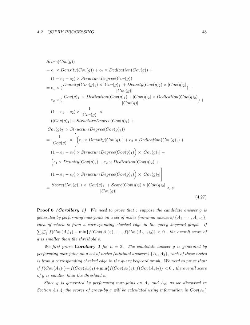
4.2. QUERY PROCESSING 48
Score(Cov(g))
= e1 ×Density(Cov(g)) + e2 ×Dedication(Cov(g)) +
(1− e1 − e2)× StructureDegree(Cov(g))
= e1 × (Density(Cov(g)1)× |Cov(g)1|+Density(Cov(g)2)× |Cov(g)2|
|Cov(g)|) +
e2 × (|Cov(g)1| ×Dedication(Cov(g)1) + |Cov(g)2| ×Dedication(Cov(g)2)
|Cov(g)|) +
(1− e1 − e2)×1
|Cov(g)|×
(|Cov(g)1| × StructureDegree(Cov(g)1) +
|Cov(g)2| × StructureDegree(Cov(g)2))
=1
|Cov(g)|×
[(e1 ×Density(Cov(g)1) + e2 ×Dedication(Cov(g)1) +
(1− e1 − e2)× StructureDegree(Cov(g)1))× |Cov(g)1|+(
e1 ×Density(Cov(g)2) + e2 ×Dedication(Cov(g)2) +
(1− e1 − e2)× StructureDegree(Cov(g)2))× |Cov(g)2|
]
=Score(Cov(g)1)× |Cov(g)1|+ Score(Cov(g)2)× |Cov(g)2|
|Cov(g)|< s
(4.27)
Proof 6 (Corollary 1) We need to prove that : suppose the candidate answer g is
generated by performing max-joins on a set of nodes (minimal answers) A1, · · · , An−1,each of which is from a corresponding checked edge in the query keyword graph. If∑n−1
i=1 f(Cov(Ai)1) + minf(Cov(A1)2), · · · , f(Cov(An−1)2) < 0 , the overall score of
g is smaller than the threshold s.
We first prove Corollary 1 for n = 3. The candidate answer g is generated by
performing max-joins on a set of nodes (minimal answers) A1, A2, each of these nodes
is from a corresponding checked edge in the query keyword graph. We need to prove that:
if f(Cov(A1)1)+f(Cov(A2)1)+minf(Cov(A1)2), f(Cov(A2)2) < 0 , the overall score
of g is smaller than the threshold s.
Since g is generated by performing max-joins on A1 and A2, as we discussed in
Section 4.1.4, the scores of group-by g will be calculated using information in Cov(A1)
CHAPTER 4. THE TOP-K ALGORITHM 49
⋃Cov(A2). So we have:
f(Cov(g)1) = f(Cov(A1)1⋃Cov(A2)1) ≤ f(Cov(A1)1) + f(Cov(A2)1)
f(Cov(g)2) = f(Cov(A1)2⋃Cov(A2)2) ≤ minCov(A1)2, Cov(A2)2
(4.28)
So we have:
f(Cov(g)1) + f(Cov(g)2)
≤ f(Cov(A1)1) + f(Cov(A2)1) +minCov(A1)2, Cov(A2)2 < 0
(4.29)
According to Theorem 3, we proved that the overall score of g is smaller than the
threshold s. Similarly, we can prove Corollary 1 for n ≥ 4:
f(Cov(g)1) = f(Cov(A1)1⋃· · ·⋃Cov(A2)1) ≤ f(Cov(A1)1) + · · ·+ f(Cov(A2)1)
f(Cov(g)2) = f(Cov(A1)2⋃· · ·⋃Cov(A2)2) ≤ minCov(A1)2, · · · , Cov(A2)2
(4.30)
f(Cov(g)1) + f(Cov(g)2)
≤ f(Cov(A1)1) + · · ·+ f(Cov(A2)1) +minCov(A1)2, · · · , Cov(A2)2 < 0
(4.31)
Example 11 (The pruning step) In the scenario of the above example, two white
nodes of edge (w1, w2) and one white node of edge (w2, w3) are detected in the bounding
step (Figure 4.8). In the pruning step, more white nodes can be detected using Corollary
1.
First, we detect more white nodes for edge (w2, w3).
• Create two sets, S1 and S2.
• For each checked edge, if the edge is not (w2, w3) and suppose its associated
white nodes are B1, · · · , Bh, 1) we scan these white nodes and record max
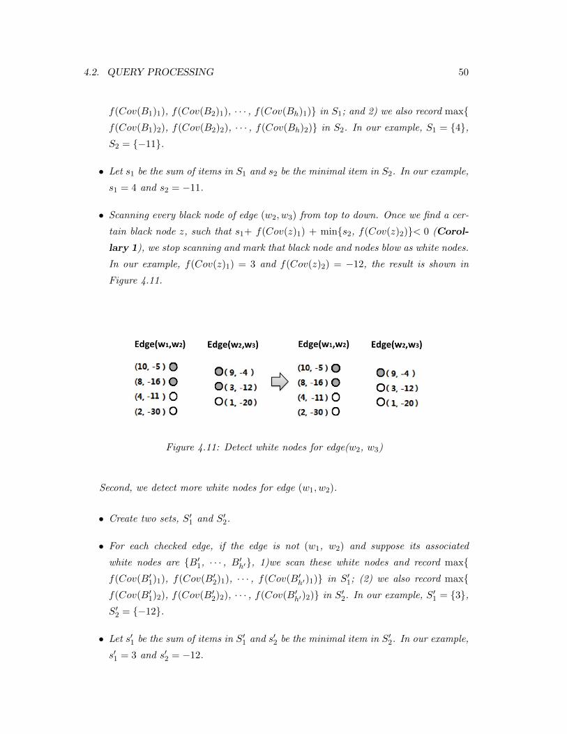
4.2. QUERY PROCESSING 50
f(Cov(B1)1), f(Cov(B2)1), · · · , f(Cov(Bh)1) in S1; and 2) we also record maxf(Cov(B1)2), f(Cov(B2)2), · · · , f(Cov(Bh)2) in S2. In our example, S1 = 4,S2 = −11.
• Let s1 be the sum of items in S1 and s2 be the minimal item in S2. In our example,
s1 = 4 and s2 = −11.
• Scanning every black node of edge (w2, w3) from top to down. Once we find a cer-
tain black node z, such that s1+ f(Cov(z)1) + mins2, f(Cov(z)2)< 0 (Corol-
lary 1), we stop scanning and mark that black node and nodes blow as white nodes.
In our example, f(Cov(z)1) = 3 and f(Cov(z)2) = −12, the result is shown in
Figure 4.11.
Figure 4.11: Detect white nodes for edge(w2, w3)
Second, we detect more white nodes for edge (w1, w2).
• Create two sets, S′1 and S′2.
• For each checked edge, if the edge is not (w1, w2) and suppose its associated
white nodes are B′1, · · · , B′h′, 1)we scan these white nodes and record maxf(Cov(B′1)1), f(Cov(B′2)1), · · · , f(Cov(B′h′)1) in S′1; (2) we also record maxf(Cov(B′1)2), f(Cov(B′2)2), · · · , f(Cov(B′h′)2) in S′2. In our example, S′1 = 3,S′2 = −12.
• Let s′1 be the sum of items in S′1 and s′2 be the minimal item in S′2. In our example,
s′1 = 3 and s′2 = −12.
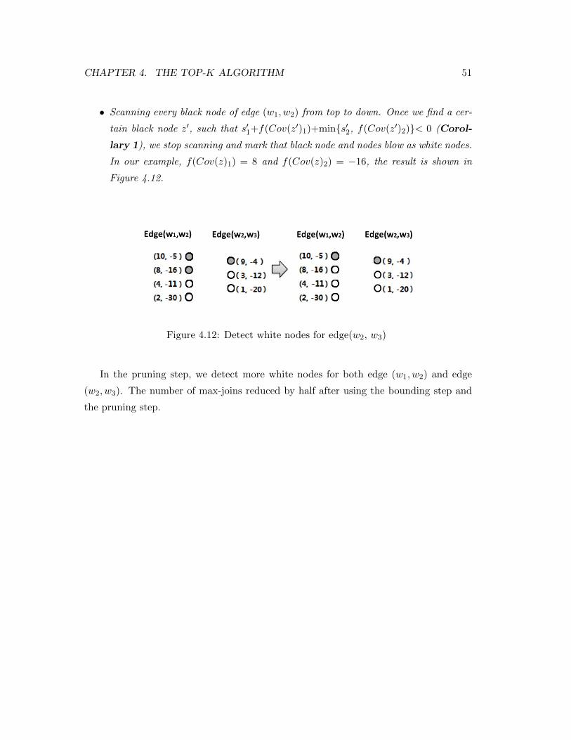
CHAPTER 4. THE TOP-K ALGORITHM 51
• Scanning every black node of edge (w1, w2) from top to down. Once we find a cer-
tain black node z′, such that s′1+f(Cov(z′)1)+mins′2, f(Cov(z′)2)< 0 (Corol-
lary 1), we stop scanning and mark that black node and nodes blow as white nodes.
In our example, f(Cov(z)1) = 8 and f(Cov(z)2) = −16, the result is shown in
Figure 4.12.
Figure 4.12: Detect white nodes for edge(w2, w3)
In the pruning step, we detect more white nodes for both edge (w1, w2) and edge
(w2, w3). The number of max-joins reduced by half after using the bounding step and
the pruning step.
Chapter 5
Experimental Results
In this section, we report an empirical study of our top-k query answering method on
two real data sets. We first describe the user study which is used to learn the coefficients
for the overall scoring function. Then, we report the effectiveness of the bounding step
and the pruning step. Finally, we evaluate the top-k query answering method and the
complete query answering method under various number of tuples and dimensions.
5.1 Environments and Data Sets
All the experiments were conducted on a PC computer running the Microsoft Windows
7 Professional Edition operating system, with a 2.4 GHz CPU, 2.0 GB main memory,
and a 250 GB hard disk. The programs were implemented in JAVA (JDK 1.6) and were
compiled using eclipse 3.7.0.
The e-Fashion dataset and the SuperstoreSales dataset have been used in example
projects of SAP on keyword search on relational databases. Since our project is sup-
ported by SAP, we use these two datasets to empirically evaluate our aggregate keyword
search methods. The dimensions of the e-Fashion dataset are shown in Table 5.1. There
are 9 dimensions, 4300 tuples and 4000 unique keywords in the e-Fashion dataset. The
SuperstoreSales dataset has 21 dimensions, 8339 tuples and 0.35 million unique key-
words. Table 5.2 shows the dimensions in the SuperstoreSales dataset. To keep our
discussion simple, we assume all the database fields are text attributes. In data rep-
resentation, we adopted the popular packing technique [3]. A value on a dimension is
mapped to an integer. The star value on a dimension is mapped to 0. We also map
keywords to integers.
52
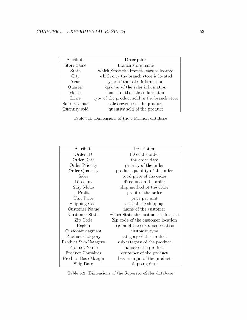
CHAPTER 5. EXPERIMENTAL RESULTS 53
Attribute Description
Store name branch store nameState which State the branch store is locatedCity which city the branch store is locatedYear year of the sales information
Quarter quarter of the sales informationMonth month of the sales informationLines type of the product sold in the branch store
Sales revenue sales revenue of the productQuantity sold quantity sold of the product
Table 5.1: Dimensions of the e-Fashion database
Attribute Description
Order ID ID of the orderOrder Date the order date
Order Priority priority of the orderOrder Quantity product quantity of the order
Sales total price of the orderDiscount discount on the order
Ship Mode ship method of the orderProfit profit of the order
Unit Price price per unitShipping Cost cost of the shipping
Customer Name name of the customerCustomer State which State the customer is located
Zip Code Zip code of the customer locationRegion region of the customer location
Customer Segment customer typeProduct Category category of the product
Product Sub-Category sub-category of the productProduct Name name of the product
Product Container container of the productProduct Base Margin base margin of the product
Ship Date shipping date
Table 5.2: Dimensions of the SuperstoreSales database

5.2. USER STUDY 54
5.2 User Study
We use the traditional linear regression model [10, 8] to learn the ranking function. A
user study is then performed to calculate the coefficients of the overall scoring function.
For each tested query, we randomly select 5 answers for users to evaluate. For each
selected answer xi, its density score (xi1), dedication score (xi2) and structure degree
(xi3) are pre-calculated. Let yi be the score evaluated by users for the answer xi, we
have the following linear regression model:
f(xi) = e1 × xi1 + e2 × xi2 + (1− e1 − e2)× xi3
(5.1)
The minimum sum of squares (SSE, the error sum of squares) we used in the learning
model is:
SSE =
m∑i=1
(yi − f(xi))2
(5.2)
where m is the total number of selected answers evaluated by users.
In the user study, we designed three types of tested queries, each of which represents
a possible search intension. For example, given a query Q = (D,C, w1, w2, w3), it may
have the following search intensions:
1) “w1 or w2 or w3” (Table 5.3)
2) “w1 and w2 and w3” (Table 5.5)
3) Others, i.e. “w1 and w2 OR w1 and w3” (Table 5.7)
For each type of query, we test 10 instance queries. We have 10 people participating
in the studies. We get 10 sets of results, each of which is from a single user and can be
used to calculate a set of values of the coefficients. We also mix all the results from the
users and get another set of values of the coefficients. So, we have 11 sets of values of
the coefficients, as shown in Table 5.9 and Table 5.10.
The learning results may not be the best, since there are only 10 people in the user
study and we only select 5 answers randomly for each tested query. We will get better
coefficients if we have larger samples and more people.
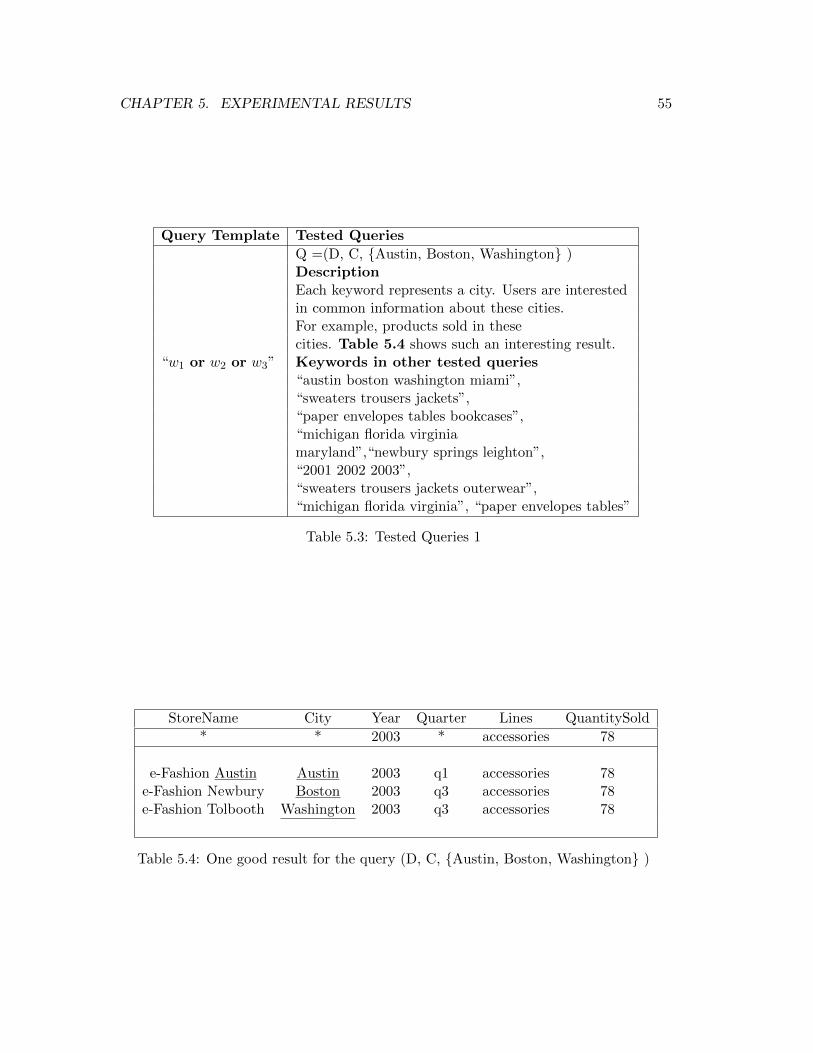
CHAPTER 5. EXPERIMENTAL RESULTS 55
Query Template Tested Queries
Q =(D, C, Austin, Boston, Washington )DescriptionEach keyword represents a city. Users are interestedin common information about these cities.For example, products sold in thesecities. Table 5.4 shows such an interesting result.
“w1 or w2 or w3” Keywords in other tested queries“austin boston washington miami”,“sweaters trousers jackets”,“paper envelopes tables bookcases”,“michigan florida virginiamaryland”,“newbury springs leighton”,“2001 2002 2003”,“sweaters trousers jackets outerwear”,“michigan florida virginia”, “paper envelopes tables”
Table 5.3: Tested Queries 1
StoreName City Year Quarter Lines QuantitySold
* * 2003 * accessories 78
e-Fashion Austin Austin 2003 q1 accessories 78e-Fashion Newbury Boston 2003 q3 accessories 78e-Fashion Tolbooth Washington 2003 q3 accessories 78
Table 5.4: One good result for the query (D, C, Austin, Boston, Washington )
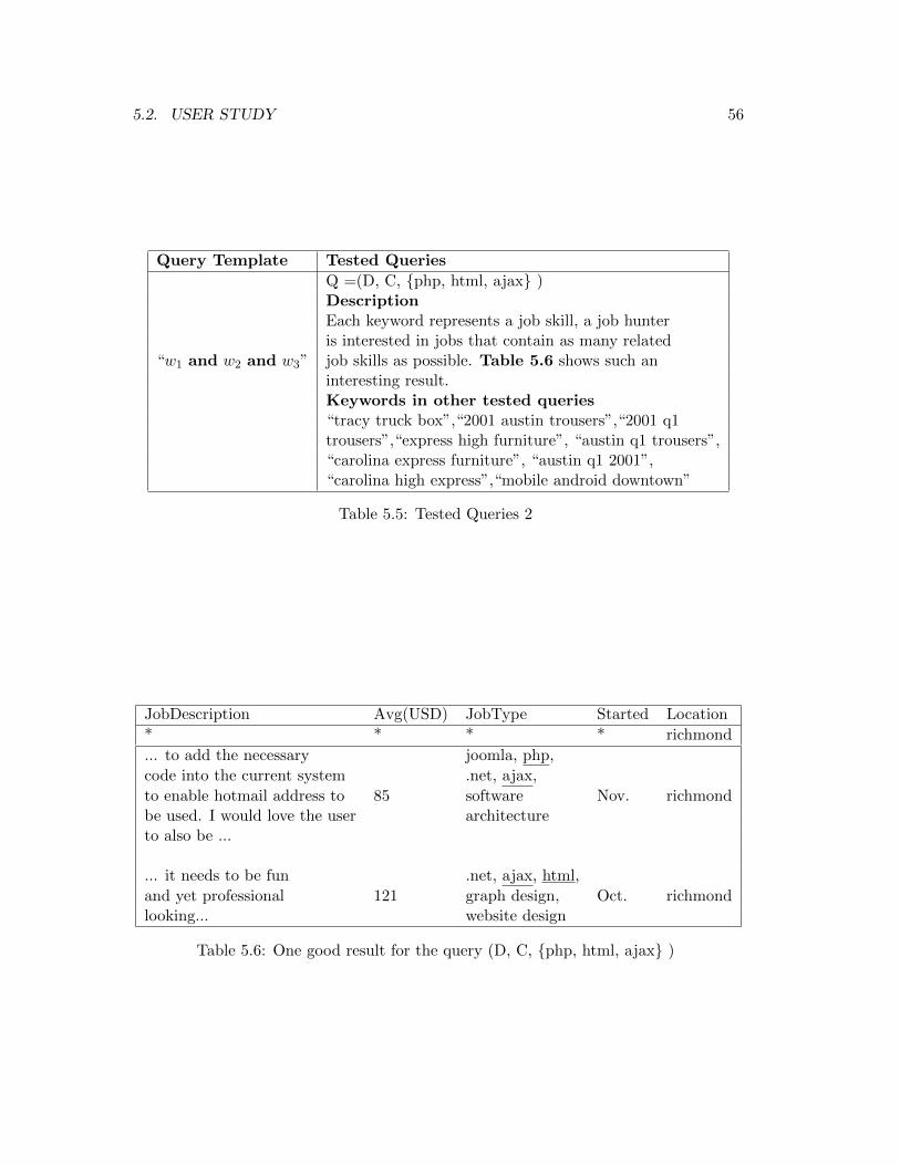
5.2. USER STUDY 56
Query Template Tested Queries
Q =(D, C, php, html, ajax )DescriptionEach keyword represents a job skill, a job hunteris interested in jobs that contain as many related
“w1 and w2 and w3” job skills as possible. Table 5.6 shows such aninteresting result.Keywords in other tested queries“tracy truck box”,“2001 austin trousers”,“2001 q1trousers”,“express high furniture”, “austin q1 trousers”,“carolina express furniture”, “austin q1 2001”,“carolina high express”,“mobile android downtown”
Table 5.5: Tested Queries 2
JobDescription Avg(USD) JobType Started Location
* * * * richmond
... to add the necessary joomla, php,
code into the current system .net, ajax,
to enable hotmail address to 85 software Nov. richmondbe used. I would love the user architectureto also be ...
... it needs to be fun .net, ajax, html,
and yet professional 121 graph design, Oct. richmondlooking... website design
Table 5.6: One good result for the query (D, C, php, html, ajax )
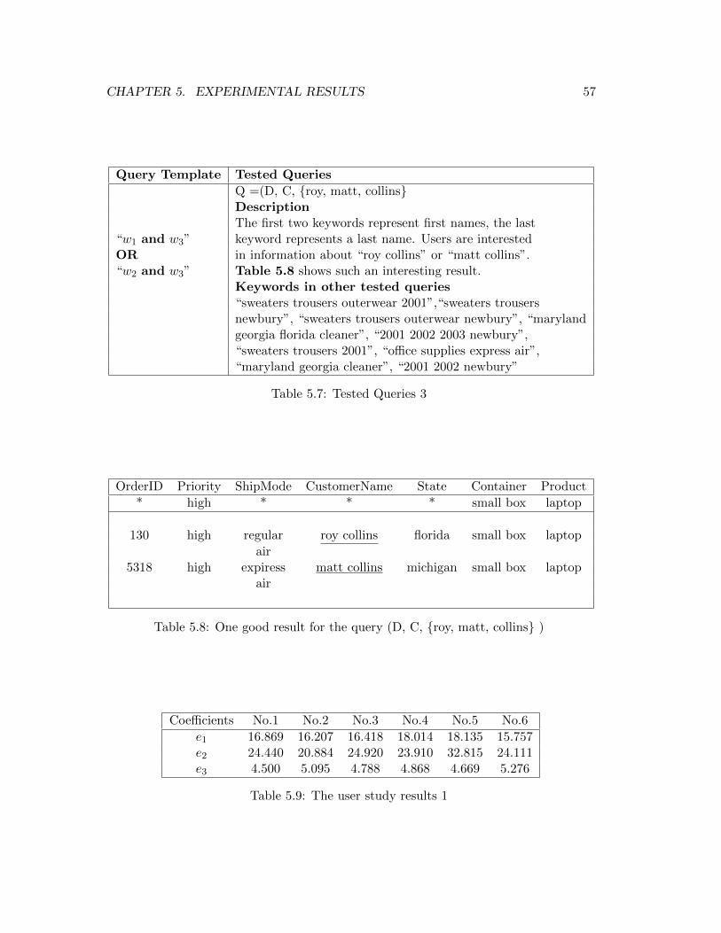
CHAPTER 5. EXPERIMENTAL RESULTS 57
Query Template Tested Queries
Q =(D, C, roy, matt, collinsDescriptionThe first two keywords represent first names, the last
“w1 and w3” keyword represents a last name. Users are interestedOR in information about “roy collins” or “matt collins”.“w2 and w3” Table 5.8 shows such an interesting result.
Keywords in other tested queries“sweaters trousers outerwear 2001”,“sweaters trousersnewbury”, “sweaters trousers outerwear newbury”, “marylandgeorgia florida cleaner”, “2001 2002 2003 newbury”,“sweaters trousers 2001”, “office supplies express air”,“maryland georgia cleaner”, “2001 2002 newbury”
Table 5.7: Tested Queries 3
OrderID Priority ShipMode CustomerName State Container Product
* high * * * small box laptop
130 high regular roy collins florida small box laptop
air5318 high expiress matt collins michigan small box laptop
air
Table 5.8: One good result for the query (D, C, roy, matt, collins )
Coefficients No.1 No.2 No.3 No.4 No.5 No.6
e1 16.869 16.207 16.418 18.014 18.135 15.757e2 24.440 20.884 24.920 23.910 32.815 24.111e3 4.500 5.095 4.788 4.868 4.669 5.276
Table 5.9: The user study results 1
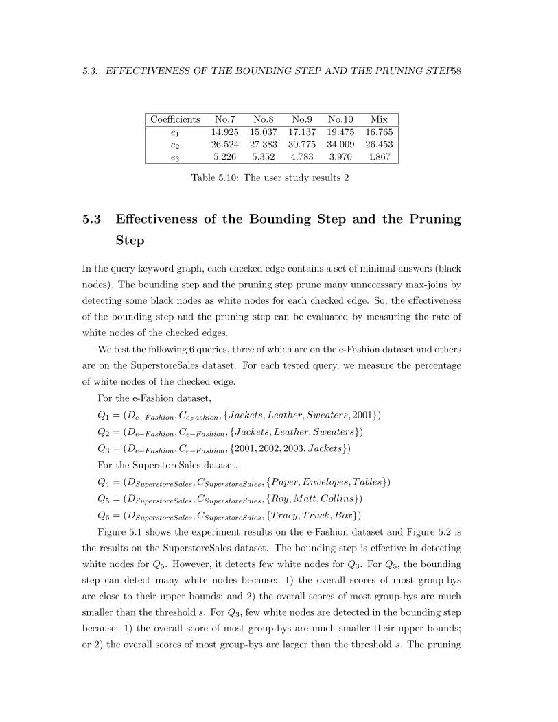
5.3. EFFECTIVENESS OF THE BOUNDING STEP AND THE PRUNING STEP58
Coefficients No.7 No.8 No.9 No.10 Mix
e1 14.925 15.037 17.137 19.475 16.765e2 26.524 27.383 30.775 34.009 26.453e3 5.226 5.352 4.783 3.970 4.867
Table 5.10: The user study results 2
5.3 Effectiveness of the Bounding Step and the Pruning
Step
In the query keyword graph, each checked edge contains a set of minimal answers (black
nodes). The bounding step and the pruning step prune many unnecessary max-joins by
detecting some black nodes as white nodes for each checked edge. So, the effectiveness
of the bounding step and the pruning step can be evaluated by measuring the rate of
white nodes of the checked edges.
We test the following 6 queries, three of which are on the e-Fashion dataset and others
are on the SuperstoreSales dataset. For each tested query, we measure the percentage
of white nodes of the checked edge.
For the e-Fashion dataset,
Q1 = (De−Fashion, CeF ashion, Jackets, Leather, Sweaters, 2001)Q2 = (De−Fashion, Ce−Fashion, Jackets, Leather, Sweaters)Q3 = (De−Fashion, Ce−Fashion, 2001, 2002, 2003, Jackets)For the SuperstoreSales dataset,
Q4 = (DSuperstoreSales, CSuperstoreSales, Paper,Envelopes, Tables)Q5 = (DSuperstoreSales, CSuperstoreSales, Roy,Matt, Collins)Q6 = (DSuperstoreSales, CSuperstoreSales, Tracy, Truck,Box)Figure 5.1 shows the experiment results on the e-Fashion dataset and Figure 5.2 is
the results on the SuperstoreSales dataset. The bounding step is effective in detecting
white nodes for Q5. However, it detects few white nodes for Q3. For Q5, the bounding
step can detect many white nodes because: 1) the overall scores of most group-bys
are close to their upper bounds; and 2) the overall scores of most group-bys are much
smaller than the threshold s. For Q3, few white nodes are detected in the bounding step
because: 1) the overall score of most group-bys are much smaller their upper bounds;
or 2) the overall scores of most group-bys are larger than the threshold s. The pruning

CHAPTER 5. EXPERIMENTAL RESULTS 59
Figure 5.1: Effectiveness of the bounding step and the pruning step on the e-Fashiondataset
Figure 5.2: Effectiveness of the bounding step and the pruning step on the Superstore-Sales dataset
5.4. THE TOP-K QUERY ANSWERING METHOD 60
step is designed to detect more white nodes for each checked edge. After using the
pruning step, we get better results. The pruning step detects many white nodes for all
tested queries. For Q3, about 90% of the nodes are detected as white nodes after the
pruning step. For Q2, although there is no big improvement after the pruning step, the
result is still better than previous. In the pruning step, each group-by’s covered tuples
are divides into two types: 1) tuples with overall scores smaller than the threshold s
and 2) tuples with overall scores not smaller than s. Such information can help better
predicting if the overall score of a group-by is smaller than the threshold s.
5.4 The Top-k Query Answering Method
We use the e-Fashion dataset and the SuperstoreSales dataset to study the efficiency
of the top-k query answering method. To study the scalability of our algorithm, we
measure the query answering time of our method under various number of tuples and
dimensions in the datasets.
We conduct two query answering experiments on the datasets. In our experiments,
the top-k query answering method returns top-10 answers. In the first experiment, we
change the number of tuples in the datasets. The corresponding results are shown in
Figure 5.3 and Figure 5.4. For the complete query answering method, increasing the
number of tuples results in a fairly linear increase in the runtime. One reason is that the
number of max-join operations increases with the number of tuples. Another reason is
that there could be more answers if the datasets contains more tuples. The top-k query
answering method is also sensitive to the number of tuples in the datasets, but it is faster
than the complete query answering method. The reason is that many unnecessary max-
join operations in the top-k query answering method are pruned after the bounding step
and the pruning step. As the number of tuples increases, more unnecessary joins are
pruned and the top-k query answering method performs better than the complete query
answering method.
In the second experiment, we change the number of dimensions in the datasets. The
corresponding results are shown in Figure 5.5 and Figure 5.6. The result of the second
experiment is similar with that of the first experiment. When the number of dimensions
increases, both the top-k query answering method and the complete query answering
method spend longer time to find the answers. One reason is that when there are more
dimensions in the datasets, the number of max-join operations does not increase but it
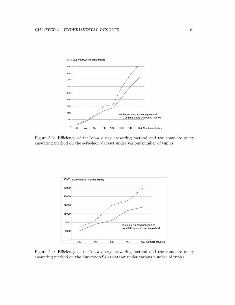
CHAPTER 5. EXPERIMENTAL RESULTS 61
Figure 5.3: Efficiency of theTop-k query answering method and the complete queryanswering method on the e-Fashion dataset under various number of tuples
Figure 5.4: Efficiency of theTop-k query answering method and the complete queryanswering method on the SuperstoreSales dataset under various number of tuples

5.4. THE TOP-K QUERY ANSWERING METHOD 62
Figure 5.5: Efficiency of theTop-k query answering method and the complete queryanswering method on the e-Fashion dataset under various number of dimensions
Figure 5.6: Efficiency of theTop-k query answering method and the complete queryanswering method on the SuperstoreSales dataset under various number of dimensions
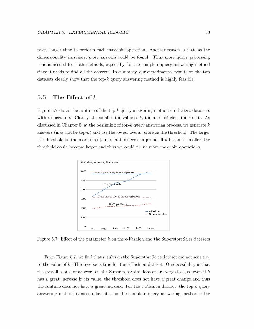
CHAPTER 5. EXPERIMENTAL RESULTS 63
takes longer time to perform each max-join operation. Another reason is that, as the
dimensionality increases, more answers could be found. Thus more query processing
time is needed for both methods, especially for the complete query answering method
since it needs to find all the answers. In summary, our experimental results on the two
datasets clearly show that the top-k query answering method is highly feasible.
5.5 The Effect of k
Figure 5.7 shows the runtime of the top-k query answering method on the two data sets
with respect to k. Clearly, the smaller the value of k, the more efficient the results. As
discussed in Chapter 5, at the beginning of top-k query answering process, we generate k
answers (may not be top-k) and use the lowest overall score as the threshold. The larger
the threshold is, the more max-join operations we can prune. If k becomes smaller, the
threshold could become larger and thus we could prune more max-join operations.
Figure 5.7: Effect of the parameter k on the e-Fashion and the SuperstoreSales datasets
From Figure 5.7, we find that results on the SuperstoreSales dataset are not sensitive
to the value of k. The reverse is true for the e-Fashion dataset. One possibility is that
the overall scores of answers on the SuperstoreSales dataset are very close, so even if k
has a great increase in its value, the threshold does not have a great change and thus
the runtime does not have a great increase. For the e-Fashion dataset, the top-k query
answering method is more efficient than the complete query answering method if the

5.5. THE EFFECT OF K 64
value of k is small (< 80). For the SuperstoreSales dataset, the top-k query answering
method is more efficient than the complete query answering method for most values of
k.
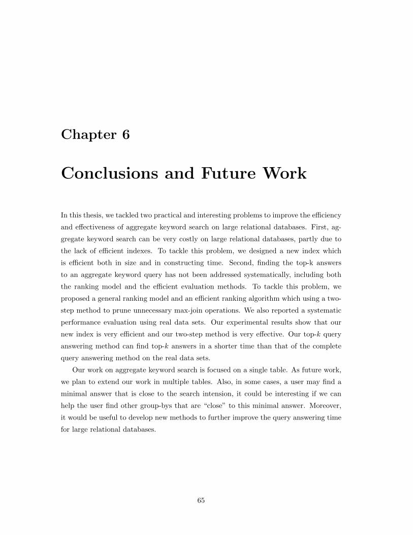
Chapter 6
Conclusions and Future Work
In this thesis, we tackled two practical and interesting problems to improve the efficiency
and effectiveness of aggregate keyword search on large relational databases. First, ag-
gregate keyword search can be very costly on large relational databases, partly due to
the lack of efficient indexes. To tackle this problem, we designed a new index which
is efficient both in size and in constructing time. Second, finding the top-k answers
to an aggregate keyword query has not been addressed systematically, including both
the ranking model and the efficient evaluation methods. To tackle this problem, we
proposed a general ranking model and an efficient ranking algorithm which using a two-
step method to prune unnecessary max-join operations. We also reported a systematic
performance evaluation using real data sets. Our experimental results show that our
new index is very efficient and our two-step method is very effective. Our top-k query
answering method can find top-k answers in a shorter time than that of the complete
query answering method on the real data sets.
Our work on aggregate keyword search is focused on a single table. As future work,
we plan to extend our work in multiple tables. Also, in some cases, a user may find a
minimal answer that is close to the search intension, it could be interesting if we can
help the user find other group-bys that are “close” to this minimal answer. Moreover,
it would be useful to develop new methods to further improve the query answering time
for large relational databases.
65

Appendix A
A.1 The proof of Equation 4.8 in Chapter 4
Suppose there are n edges in the query keyword graph and thus we need to check n− 1
edges to generate all the candidate answers. To generate one candidate answer g, we
need to perform max-joins on a set of nodes A1, · · · , An−1, where Ai is a node from a
corresponding checked edge. For simplicity, suppose n = 2 and g is the max-join result
of nodes (group-bys) A1 and A2. The best upper bound of g’s dedication score is:
Dedication(A1) +Dedication(A2) (4.8)
Proof 7 (Equation 4.8) Suppose: 1) there are M rows in Cov(A1)⋃Cov(A2), the
dedication scores of these rows are d1, · · · , dM ; 2) there are N ′ rows in Cov(A1) −Cov(A1)
⋃Cov(A2), the dedication scores of these rows are a1, · · · , aN ′; and 3) there
are N ′′ rows in Cov(A2)− Cov(A1)⋃Cov(A2), the dedication scores of these rows are
b1, · · · , bN ′′. So we have:
66
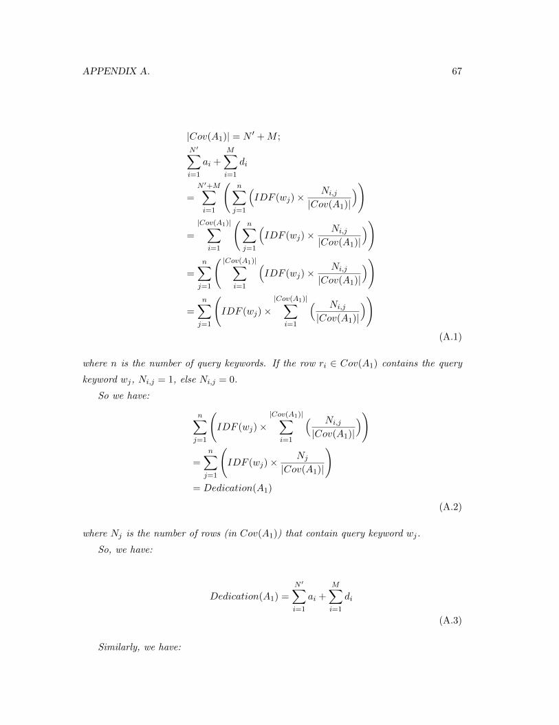
APPENDIX A. 67
|Cov(A1)| = N ′ +M ;
N ′∑i=1
ai +M∑i=1
di
=N ′+M∑i=1
(n∑
j=1
(IDF (wj)×
Ni,j
|Cov(A1)|
))
=
|Cov(A1)|∑i=1
(n∑
j=1
(IDF (wj)×
Ni,j
|Cov(A1)|
))
=
n∑j=1
( |Cov(A1)|∑i=1
(IDF (wj)×
Ni,j
|Cov(A1)|
))
=n∑
j=1
(IDF (wj)×
|Cov(A1)|∑i=1
( Ni,j
|Cov(A1)|
))(A.1)
where n is the number of query keywords. If the row ri ∈ Cov(A1) contains the query
keyword wj, Ni,j = 1, else Ni,j = 0.
So we have:
n∑j=1
(IDF (wj)×
|Cov(A1)|∑i=1
( Ni,j
|Cov(A1)|
))
=n∑
j=1
(IDF (wj)×
Nj
|Cov(A1)|
)= Dedication(A1)
(A.2)
where Nj is the number of rows (in Cov(A1)) that contain query keyword wj.
So, we have:
Dedication(A1) =
N ′∑i=1
ai +
M∑i=1
di
(A.3)
Similarly, we have:
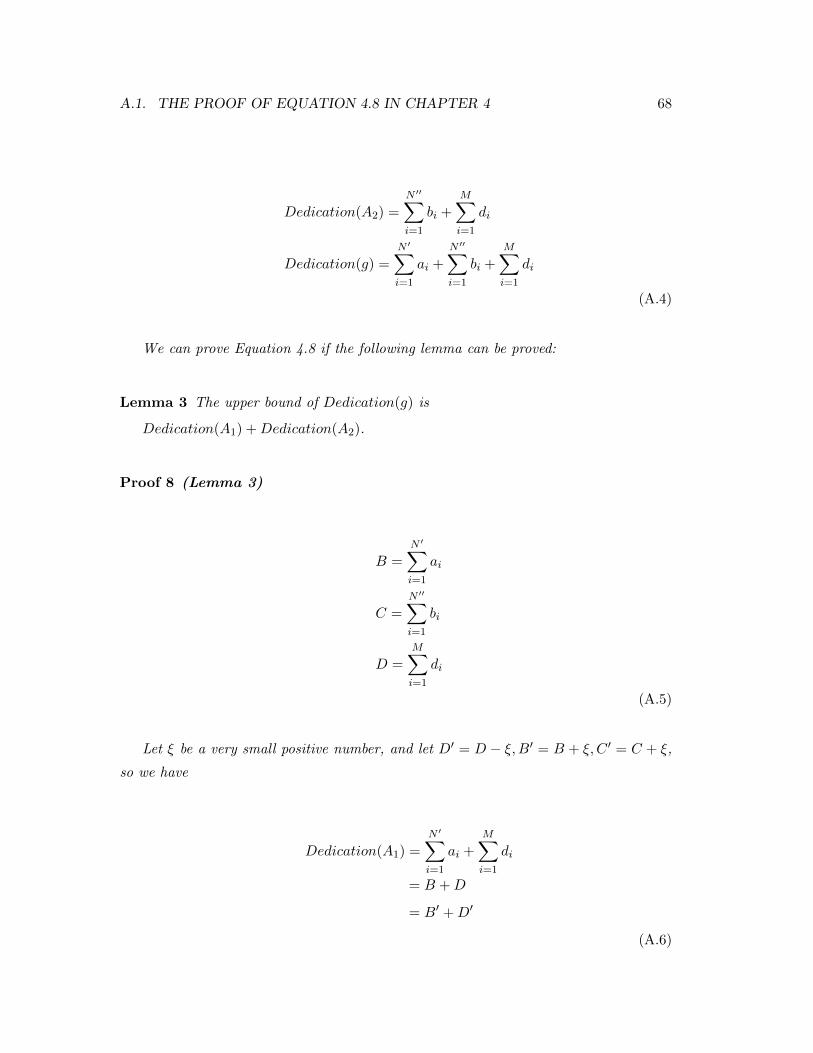
A.1. THE PROOF OF EQUATION 4.8 IN CHAPTER 4 68
Dedication(A2) =N ′′∑i=1
bi +M∑i=1
di
Dedication(g) =
N ′∑i=1
ai +
N ′′∑i=1
bi +
M∑i=1
di
(A.4)
We can prove Equation 4.8 if the following lemma can be proved:
Lemma 3 The upper bound of Dedication(g) is
Dedication(A1) +Dedication(A2).
Proof 8 (Lemma 3)
B =N ′∑i=1
ai
C =
N ′′∑i=1
bi
D =M∑i=1
di
(A.5)
Let ξ be a very small positive number, and let D′ = D − ξ,B′ = B + ξ, C ′ = C + ξ,
so we have
Dedication(A1) =N ′∑i=1
ai +M∑i=1
di
= B +D
= B′ +D′
(A.6)
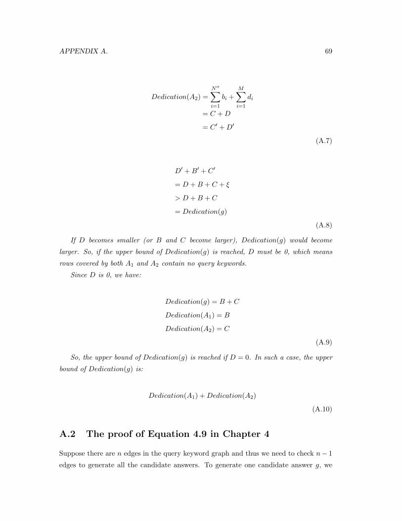
APPENDIX A. 69
Dedication(A2) =N ′′∑i=1
bi +M∑i=1
di
= C +D
= C ′ +D′
(A.7)
D′ +B′ + C ′
= D +B + C + ξ
> D +B + C
= Dedication(g)
(A.8)
If D becomes smaller (or B and C become larger), Dedication(g) would become
larger. So, if the upper bound of Dedication(g) is reached, D must be 0, which means
rows covered by both A1 and A2 contain no query keywords.
Since D is 0, we have:
Dedication(g) = B + C
Dedication(A1) = B
Dedication(A2) = C
(A.9)
So, the upper bound of Dedication(g) is reached if D = 0. In such a case, the upper
bound of Dedication(g) is:
Dedication(A1) +Dedication(A2)
(A.10)
A.2 The proof of Equation 4.9 in Chapter 4
Suppose there are n edges in the query keyword graph and thus we need to check n− 1
edges to generate all the candidate answers. To generate one candidate answer g, we
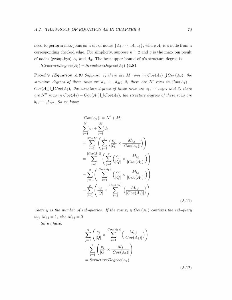
A.2. THE PROOF OF EQUATION 4.9 IN CHAPTER 4 70
need to perform max-joins on a set of nodes A1, · · · , An−1, where Ai is a node from a
corresponding checked edge. For simplicity, suppose n = 2 and g is the max-join result
of nodes (group-bys) A1 and A2. The best upper bound of g’s structure degree is:
StructureDegree(A1) + StructureDegree(A2) (4.8)
Proof 9 (Equation 4.9) Suppose: 1) there are M rows in Cov(A1)⋃Cov(A2), the
structure degrees of these rows are d1, · · · , dM ; 2) there are N ′ rows in Cov(A1) −Cov(A1)
⋃Cov(A2), the structure degrees of these rows are a1, · · · , aN ′; and 3) there
are N ′′ rows in Cov(A2)− Cov(A1)⋃Cov(A2), the structure degrees of these rows are
b1, · · · , bN ′′. So we have:
|Cov(A1)| = N ′ +M ;
N ′∑i=1
ai +M∑i=1
di
=N ′+M∑i=1
(y∑
j=1
( cj|Q|× Mi,j
|Cov(A1)|
))
=
|Cov(A1)|∑i=1
(y∑
j=1
( cj|Q|× Mi,j
|Cov(A1)|
))
=
y∑j=1
( |Cov(A1)|∑i=1
( cj|Q|× Mi,j
|Cov(A1)|
))
=
y∑j=1
(cj|Q|×|Cov(A1)|∑
i=1
( Mi,j
|Cov(A1)|
))(A.11)
where y is the number of sub-queries. If the row ri ∈ Cov(A1) contains the sub-query
wj, Mi,j = 1, else Mi,j = 0.
So we have:
y∑j=1
(cj|Q|×|Cov(A1)|∑
i=1
( Mi,j
|Cov(A1)|
))
=
y∑j=1
(cj|Q|× Mj
|Cov(A1)|
)= StructureDegree(A1)
(A.12)
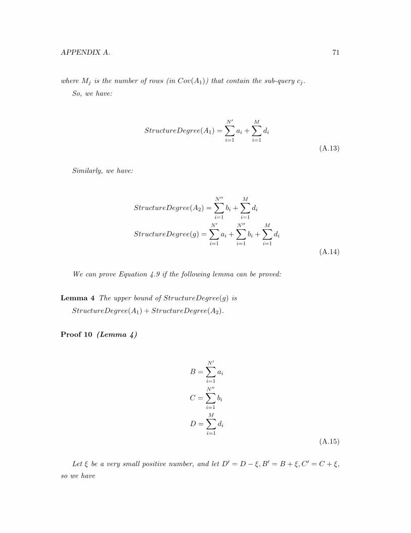
APPENDIX A. 71
where Mj is the number of rows (in Cov(A1)) that contain the sub-query cj.
So, we have:
StructureDegree(A1) =
N ′∑i=1
ai +
M∑i=1
di
(A.13)
Similarly, we have:
StructureDegree(A2) =N ′′∑i=1
bi +M∑i=1
di
StructureDegree(g) =N ′∑i=1
ai +N ′′∑i=1
bi +M∑i=1
di
(A.14)
We can prove Equation 4.9 if the following lemma can be proved:
Lemma 4 The upper bound of StructureDegree(g) is
StructureDegree(A1) + StructureDegree(A2).
Proof 10 (Lemma 4)
B =N ′∑i=1
ai
C =
N ′′∑i=1
bi
D =
M∑i=1
di
(A.15)
Let ξ be a very small positive number, and let D′ = D − ξ,B′ = B + ξ, C ′ = C + ξ,
so we have
A.2. THE PROOF OF EQUATION 4.9 IN CHAPTER 4 72
StructureDegree(A1) =N ′∑i=1
ai +M∑i=1
di
= B +D
= B′ +D′
(A.16)
StructureDegree(A2) =N ′′∑i=1
bi +M∑i=1
di
= C +D
= C ′ +D′
(A.17)
D′ +B′ + C ′
= D +B + C + ξ
> D +B + C
= StructureDegree(g)
(A.18)
If D becomes smaller (or B and C become larger), StructureDegree(g) would become
larger. So, if the upper bound of StructureDegree(g) is reached, D must be 0, which
means rows covered by both A1 and A2 contain no query keywords.
Since D is 0, we have:
StructureDegree(g) = B + C
StructureDegree(A1) = B
StructureDegree(A2) = C
(A.19)
So, the upper bound of StructureDegree(g) is reached if D = 0. In such a case, the
upper bound of StructureDegree(g) is:

APPENDIX A. 73
StructureDegree(A1) + StructureDegree(A2)
(A.20)

Bibliography
[1] Sanjay Agrawal, Surajit Chaudhuri, and Gautam Das. Dbxplorer: A system forkeyword-based search over relational databases. In Proceedings of the 18th Interna-tional Conference on Data Engineering, ICDE 2002, 26 February - 1 March 2002,San Jose, CA, pages 5–16. IEEE Computer Society, 2002.
[2] Andrey Balmin, Vagelis Hristidis, and Yannis Papakonstantinou. Objectrank:Authority-based keyword search in databases. In Proceedings of the Thirtieth In-ternational Conference on Very Large Data Bases, VLDB 2004, Toronto, Canada,August 31 - September 3 2004, pages 564–575. Morgan Kaufmann, 2004.
[3] Kevin S. Beyer and Raghu Ramakrishnan. Bottom-up computation of sparse andiceberg cubes. In Proceedings ACM SIGMOD International Conference on Manage-ment of Data, SIGMOD 1999, June 1-3, 1999, Philadelphia, Pennsylvania, USA,pages 359–370. ACM Press, 1999.
[4] Gaurav Bhalotia, Arvind Hulgeri, Charuta Nakhe, Soumen Chakrabarti, and S. Su-darshan. Keyword searching and browsing in databases using banks. In Proceedingsof the 18th International Conference on Data Engineering, ICDE 2002, 26 February- 1 March 2002, San Jose, CA, pages 431–440. IEEE Computer Society, 2002.
[5] Yi Chen, Wei Wang, and Ziyang Liu. Keyword-based search and exploration ondatabases. In Proceedings of the 27th International Conference on Data Engineer-ing, ICDE 2011, April 11-16, 2011, Hannover, Germany, pages 1380–1383. IEEEComputer Society, 2011.
[6] Bolin Ding, Yintao Yu, Bo Zhao, Cindy Xide Lin, Jiawei Han, and ChengxiangZhai. Keyword search in text cube: Finding top-k aggregated cell documents. InProceedings of the 2010 Conference on Intelligent Data Understanding, CIDU 2010,October 5-6, 2010, Mountain View, California, USA, pages 145–159. NASA AmesResearch Center, 2010.
[7] Bolin Ding, Bo Zhao, Cindy Xide Lin, Jiawei Han, and Chengxiang Zhai. Topcells:Keyword-based search of top-k aggregated documents in text cube. In Proceedingsof the 26th International Conference on Data Engineering, ICDE 2010, March 1-6,2010, Long Beach, California, USA, pages 381–384. IEEE, 2010.
74

BIBLIOGRAPHY 75
[8] Norman R. Draper and Harry Smith. Applied regression analysis (2. ed.). Wileyseries in probability and mathematical statistics. Wiley, 1981.
[9] Ronald Fagin, Amnon Lotem, and Moni Naor. Optimal aggregation algorithms formiddleware. J. Comput. Syst. Sci., 66(4):614–656, 2003.
[10] Jane Fedorowicz. Database evaluation using multiple regression techniques. InProceedings of Annual Meeting, SIGMOD 1984, Boston, Massachusetts, June 18-21, 1984, pages 70–76. ACM Press, 1984.
[11] S. L. Hakimi. Steiner’s problem in graphs and its implications. Wiley Periodicals,Inc., 1(2):113–133, 1971.
[12] Vagelis Hristidis and Yannis Papakonstantinou. Discover: Keyword search in re-lational databases. In Proceedings of 28th International Conference on Very LargeData Bases, VLDB 2002, August 20-23, 2002, Hong Kong, China, pages 670–681.Morgan Kaufmann, 2002.
[13] Ihab F. Ilyas, George Beskales, and Mohamed A. Soliman. A survey of top-k queryprocessing techniques in relational database systems. ACM Comput. Surv., 40(4),2008.
[14] Marie Jacob and Zachary G. Ives. Sharing work in keyword search over databases.In Proceedings of the ACM SIGMOD International Conference on Management ofData, SIGMOD 2011, Athens, Greece, June 12-16, 2011, pages 577–588. ACM,2011.
[15] Jonathan Koren, Yi Zhang, and Xue Liu. Personalized interactive faceted search.In Proceedings of the 17th International Conference on World Wide Web, WWW2008, Beijing, China, April 21-25, 2008, pages 477–486. ACM, 2008.
[16] Zhicheng Li, Hu Xu, Yansheng Lu, and Aling Qian. Aggregate nearest keywordsearch in spatial databases. In Advances in Web Technologies and Applications,Proceedings of the 12th Asia-Pacific Web Conference, APWeb 2010, Busan, Korea,6-8 April 2010, pages 15–21. IEEE Computer Society, 2010.
[17] Lu Qin, Jeffrey Xu Yu, and Lijun Chang. Keyword search in databases: the powerof rdbms. In Proceedings of the ACM SIGMOD International Conference on Man-agement of Data, SIGMOD 2009, Providence, Rhode Island, USA, June 29 - July2, 2009, pages 681–694. ACM, 2009.
[18] Lu Qin, Jeffrey Xu Yu, and Lijun Chang. Computing structural statistics by key-words in databases. In Proceedings of the 27th International Conference on DataEngineering, ICDE 2011, April 11-16, 2011, Hannover, Germany, pages 363–374.IEEE Computer Society, 2011.
[19] Stephen E. Robertson, Steve Walker, and Micheline Hancock-Beaulieu. Okapi attrec-7: Automatic ad hoc, filtering, vlc and interactive. In Text REtrieval Confer-ence (TREC), pages 199–210, 1998.

BIBLIOGRAPHY 76
[20] Stephen E. Robertson, Steve Walker, Susan Jones, Micheline Hancock-Beaulieu,and Mike Gatford. Okapi at trec-3. In Text REtrieval Conference (TREC), pages0–, 1994.
[21] Gerard Salton and Chris Buckley. Term-weighting approaches in automatic textretrieval. Inf. Process. Manage., 24(5):513–523, 1988.
[22] Gerhard Weikum. Db&ir: both sides now. In Proceedings of the ACM SIGMODInternational Conference on Management of Data, Beijing, China, June 12-14,2007, pages 25–30. ACM, 2007.
[23] Ho Chung Wu, Robert Wing Pong Luk, Kam-Fai Wong, and Kui-Lam Kwok. Inter-preting tf-idf term weights as making relevance decisions. ACM Trans. Inf. Syst.,26(3), 2008.
[24] Ping Wu, Yannis Sismanis, and Berthold Reinwald. Towards keyword-driven ana-lytical processing. In Proceedings of the ACM SIGMOD International Conferenceon Management of Data, Beijing, China, June 12-14, 2007, pages 617–628. ACM,2007.
[25] Bo Zhao, Cindy Xide Lin, Bolin Ding, and Jiawei Han. Texplorer: keyword-basedobject search and exploration in multidimensional text databases. In Proceedingsof the 20th ACM Conference on Information and Knowledge Management, CIKM2011, Glasgow, United Kingdom, October 24-28, 2011, pages 1709–1718. ACM,2011.
[26] Bin Zhou and Jian Pei. Answering aggregate keyword queries on relationaldatabases using minimal group-bys. In Proceedings of the 12th International Confer-ence on Extending Database Technology: Advances in Database Technology, EDBT2009, Saint Petersburg, Russia, March 24-26, 2009, pages 108–119. ACM, 2009.