EFFICIENT CONVERSION BETWEENTEMPORAL GRANULARITIES

HONG LIN

July 8, 1997

TR-19

A TIMECENTER Technical Report

Title EFFICIENT CONVERSION BETWEEN TEMPORAL GRANULARI-TIES

Copyright c� 1997 HONG LIN. All rights reserved.

Author�s� HONG LIN

Publication History None

TIMECENTERParticipants

Aalborg University, DenmarkChristian S. Jensen (codirector)Michael H. B̈ohlenRenato BusattoHeidi GregersenKristian Torp

University of Arizona, USARichard T. Snodgrass (codirector)Anindya DattaSudha Ram

Individual participantsCurtis E. Dyreson, James Cook University, AustraliaKwang W. Nam, Chungbuk National University, KoreaKeun H. Ryu, Chungbuk National University, KoreaMichael D. Soo, University of South Florida, USAAndreas Steiner, ETH Zurich, SwitzerlandVassilis Tsotras, Polytechnic University, New York, USAJef Wijsen, Vrije Universiteit Brussel, Belgium

Any software made available viaTIMECENTERis provided “as is” and without anyexpress or implied warranties, including, without limitation, the implied warrantyof merchantability and fitness for a particular purpose.

The TIMECENTERicon on the cover combines two “arrows.” These “arrows” areletters in the so-calledRunealphabet used one millennium ago by the Vikings, aswell as by their precedessors and successors. The Rune alphabet (second phase)has 16 letters, all of which have angular shapes and lack horizontal lines becausethe primary storage medium was wood. Runes may also be found on jewelry, tools,and weapons and were perceived by many as having magic, hidden powers.

The two Rune arrows in the icon denote “T” and “C,” respectively.

EFFICIENT CONVERSION BETWEEN TEMPORALGRANULARITIES

HONG LIN, M.S.The University of Arizona, 1997

Director:

A temporal granularityis a unit of measuring time, e.g., second, day, week. Agranularity graph is a directedgraph showing the relationship among the granularities. Efficiently and correctly converting time values withinthe granularity graph is critical for supporting multiple time granularities in an application program or a databasemanagement system. The research involves finding an optimally efficient path in the granularity graph for any pairof granularities and developing an algorithm to perform the conversion operation between the two granularities foranchored time related values, to correctly convert a granule from a specified granularity to another granularity. Theresearch also evaluates several strategies to improve the performance of temporal operations at mixed granularities.

1

3

STATEMENT BY AUTHOR

This thesis has been submitted in partial fulfillment of requirements for an advanced degree at TheUniversity of Arizona and is deposited in the University Library to be made available to borrowers underrules of the Library.

Brief quotations from this thesis are allowable without special permission, provided that accurateacknowledgment of source is made. Requests for permission for extended quotation from or reproductionof this manuscript in whole or in part may be granted by the head of the major department or the Dean ofthe Graduate College when in his or her judgment the proposed use of the material is in the interests ofscholarship. In all other instances, however, permission must be obtained from the author.

SIGNED:

3

4

ACKNOWLEDGMENTS

I would like to express my deepest gratitude to my advisor and mentor, Professor Richard Snodgrass, forhis persistent inspiration, guidance and support. Without his encouragement and endless patience, I couldnot have written this thesis. I wish to thank Professor William Evans and Professor John Hartman for theirvaluable comments and advice, and Professor Curtis Dyreson and Kristian Torp for their constant help.

Special thanks go to my parents for their continuing encouragement and support, and to my husband,Xiaoguang, and son, Daniel, for their understanding, sacrifice and patience.

4

Contents

1 INTRODUCTION 1

2 RELATED WORK 2

3 THE GRANULARITY MODULE INTERFACE 6

4 DETERMINING THE OPTIMAL PATH 84.1 The Correct Paths� � � � � � � � � � � � � � � � � � � � � � � � � � � � � � � � � � � � � � 84.2 Extending TheDag-Shortest-PathsAlgorithm � � � � � � � � � � � � � � � � � � � � � � � � 104.3 A Dynamic Programming Algorithm� � � � � � � � � � � � � � � � � � � � � � � � � � � � � 12

5 THE Cast OPERATION 185.1 Computing The Anchor Offset� � � � � � � � � � � � � � � � � � � � � � � � � � � � � � � � 185.2 TheCastAlgorithm � � � � � � � � � � � � � � � � � � � � � � � � � � � � � � � � � � � � � 195.3 Proof Of Termination � � � � � � � � � � � � � � � � � � � � � � � � � � � � � � � � � � � � 21

6 PERFORMANCE 24

7 SUMMARY 29

A THE EXTERNAL INTERFACE 30

B THE INTERNAL DATA STRUCTURE 39

5

List of Figures

2.1 A multicalendar granularity graph� � � � � � � � � � � � � � � � � � � � � � � � � � � � � � 5

4.1 A simple granularity graph with two V-paths� � � � � � � � � � � � � � � � � � � � � � � � � 94.2 The time-lines at granularities�, �, �, � and� � � � � � � � � � � � � � � � � � � � � � � � 104.3 TheSearchPathAlgorithm � � � � � � � � � � � � � � � � � � � � � � � � � � � � � � � � � 114.4 AlgorithmFind Path � � � � � � � � � � � � � � � � � � � � � � � � � � � � � � � � � � � � 144.5 AlgorithmDo Close � � � � � � � � � � � � � � � � � � � � � � � � � � � � � � � � � � � � � 144.6 Updating the path-determining variables for theFind Path algorithm � � � � � � � � � � � 15

5.1 A granularity graph with nontermination problem� � � � � � � � � � � � � � � � � � � � � � 195.2 TheCast algorithm � � � � � � � � � � � � � � � � � � � � � � � � � � � � � � � � � � � � � 205.3 (a) A simple granularity graph. (b) The corresponding bipartite graph.� � � � � � � � � � � 22

6.1 The V-cost versus Sequence Length.� � � � � � � � � � � � � � � � � � � � � � � � � � � � � 266.2 The V-cost versus Sequence Length.� � � � � � � � � � � � � � � � � � � � � � � � � � � � � 266.3 The V-cost versus Sequence Length for DP-S.� � � � � � � � � � � � � � � � � � � � � � � � 276.4 The V-cost versus Sequence Length with Randomness=8 for EDSP-SC.� � � � � � � � � � � 286.5 The V-cost versus Degree of Randomness with Sequence Length=256 for EDSP-SC.� � � � 28

6

Abstract

A temporal granularityis a unit of measuring time, e.g., second, day, week. Agranularity graph is a directedgraph showing the relationship among the granularities. Efficiently and correctly converting time values withinthe granularity graph is critical for supporting multiple time granularities in an application program or a databasemanagement system. The research involves finding an optimally efficient path in the granularity graph for any pairof granularities and developing an algorithm to perform the conversion operation between the two granularities foranchored time related values, to correctly convert a granule from a specified granularity to another granularity. Theresearch also evaluates several strategies to improve the performance of temporal operations at mixed granularities.

Chapter 1

INTRODUCTION

Supportingmultiple calendars in database applications is a highly desirable feature. Currently, the Gregoriancalendar (with a fixed number of granularities: year, month, day, hour, and second) is the single calendaravailable in SQL-92 (Structured Query Language) for representing and manipulating time-related data. Inthe real world, there are many applications that require a wide variety of calendar support. The usageof a calendar depends on the cultural, legal and business aspects of the user. For example, the Easternworld commonly uses a lunar calendar, the US government uses a business calendar with the financial yearstarting in October, and universities generally use an academic calendar with years consisting of semestersor quarters. Today’s database systems must support conversion among these calendars.

There has been considerable research in incorporating multiple calendars into a database system. Butmost of the previous research has focused on theoretical aspects. For mixed granularities in multiplecalendars, no practical algorithm has been proposed that allows mappings to be composed automatically.

Based on the architecture first devised by Curtis Dyreson and Richard Snodgrass, with initial codingby Marshall Freiman, our work develops an efficient algorithm and provides a software module to supportconversion operations for mixed granularities, i.e., converting a granule in one granularity to a granule inanother granularity. The objective of this work is to provide an efficient and correct algorithm for supportingmultiple time granularities within an application program or a database.

This thesis is organized as follows. Chapter Two gives an overview of the related work on the mixedgranularities, including introducing the granularity graph and the initial model of converting time valuesfrom one granularity to another granularity. Chapter Three covers the granularity module interface andshows how to integrate different calendars into a single granularity graph. This chapter also points out whatthe interface needs to check to ensure the granularities declared by the user are properly defined. We examinethe paths for granule conversion in Chapter Four. We then present two recursive algorithms for finding anoptimal path and prove their correctness. We begin by giving an example to illustrate non-termination inconversion operation. We then propose a reasonable constraint to ensure termination. Finally, we present thealgorithm for the conversionoperation is presented. Chapter Six providesan empirical performance analysis,and examine the efficiency of path caching and the granularity origin offsets caching. We summarize ourwork in Chapter Seven. We include the external data structures and the detailed description of the functionsprovided by the external module in Appendix A. In addition, Appendix B gives the internal data structures.

1

Chapter 2

RELATED WORK

Since the very early days of computers, applications have had a need to represent times in stored data and tomanipulate the information. But there is no standard; every computer system invented its own convention tohandle time related data. This is clearly unacceptable. There have been several languages fully implementedto support the time related data available on commercial database management systems (DBMSs). The bestknown of these is SQL. SQL was first designed and implemented at IBM Corporation as the interface for anexperimental relational database system called system R. SQL was first standardized in 1986 and was revisedsignificantly to form the standard SQL-92 [Melton & Simon 1993]. SQL-92 includes date and time datatypes, and supports a single calendar, the Gregorian calendar. Recently, the Object Database ManagementGroup defined the ODMG-93 standard for object database management to provide for object databases whatSQL has provided for relational database [Cattell 1994]. But the time support in ODMG-93 is similar toSQL-92. Generally, the existing database software has ignored the issue of the mixed granularities or haveassumed the use of a single calendar.

Anderson [Anderson 1982] first pointed out the need to support mixed granularities. Clifford and Rao[Clifford & Rao 1987] then proposed a theoretical model of complete ordering of granularities. Wiederhold,Jajodia and Litwin [Wiederhold et al. 1991] further developed this model by adding a specific semantics fortemporal comparisons.

Temporal granularities, e.g., seconds, days, weeks, months, were initially formalized as partitions ofsome base time lines composed of indivisible time units, calledchronons(usually denoted as�), e.g.,microseconds. We slightly generalize Wang et. al.’s definition of time unit [Wang et al. 1993] to thefollowing.

Definition 2.1 A granularity� is a set of nonoverlapping and contiguous granules. Each granule has aninteger index, with the ordering of integers. We use an integer subscripted with the granularity to identifythe granule. The granularity contains�� termed anchor. Here,

� � f� � ������ ��� ��� � � �g.

The granularity chronons (�) is the smallest granularity. Each granule at a granularity corresponds toan contiguous set of chronons. To distinguish between a granule (an integer) and the sequence of chrononsthat comprise a granule, we useCHR to represent the set of chronons in a given granule.

Definition 2.2 CHR�i�� � fc�jc� is in i�g , wherei� is theith granule in granularity� andc� is achronon.

The above definitions imply the following properties.

2

3

� for chrononsc�, c��

and granulesi�, j�, c� � CHR�i��, c�� � CHR�j�� andc� � c��

impliesi� � j�.

� for chrononsc�, c�� andc���, c� � c�� � c��� , c� � CHR�i�� andc��� � CHR�i�� implies c�� �CHR�i�� .

� For granulesi� andj� , i� �� j� impliesCHR�i�� � CHR�j�� � .

The first property says that chronons and granules are totally ordered. The second one requires that a granulecontains a contiguous set of chronons and the third one ensures that the different granules do not overlap.We differ from Wang’s definition in not requiring�� � CHR���� (Business calendar has an anchor inGregorian date October 1, 1990), and in allowing gaps, i.e., some chronons may not map to any granule ofa particular granularity, e.g., semesters with no summer coverage.

Cast, which converts a granule of one granularity to a granule of another granularity, is the basicoperation on granule. Other operations (for example,Scale, Plus) generally can be defined in terms of theCast. Following is the formal definition for theCast.

Definition 2.3 Cast�i�� �� �� j� , where� and� are granularities,i� is theith granule in� andj� isthejth granule in�.

Given the definition of granularity, clearly, there is a “finer than” relation between granularities. Forexample, days is finer than months, months is finer than years, etc. Note that months is not a furtherpartitioning of weeks, or vice-versa.A complete latticeis a partially ordered set in which every pair ofelements have a unique least upper bound and a unique greatest lower bound [Vinogradov et al. 1988]. Ithas been shown that a collection of granularities (or time units) can form a complete lattice with respectto a “finer than” relationship [Wang et al. 1993]. By relating an arbitrary time unit (i.e., granularity) to thesmallest time unit (i.e., chronons), theCastoperation is easily definable (the latter because the existence ofa bottom in the lattice ensures that there is a path from a granularity to all other granularities, and the factthat the granule-chronon mapping is invertible). This model is sufficient from a mathematical point of view,but does not present a practical solution. First, most calendar users do not know what the smallest timeunit it is; they usually build a new calendar based on a well-known calendar. Second, given leap secondsand various arbitrary aspects of human-designed calendars, the mapping functions from granularities to thesmallest time unit are generally complex. Third, if a set of granularities do not form a complete lattice,one or more artificial granularities have to be added in order to form a complete lattice. These extragranularities “may sometimes be very hard to compute and counter-intuitive to real-life concepts of timeunits” [Wang et al. 1993]. Finally, this model has not considered the anchor difference between a pair ofgranularities. It assumes that all granularities have a same anchor. In reality, this assumption is impractical.At the physical level, time values are stored in fixed-size data structures called timestamps. For example, ifwe pick midnight, January 1, A.D. 1 as the anchor-point for all granularities, then representing a time valuefor Business day (starting on the Gregorian date October 1, 1990) would require many storage bits. Usingdifferent anchors can significantly reduce the storage requirement.

Although Wang’s model provides a mathematical framework for mixed granularities, they do notpresent calendars. Recently, Kraus et al. propose a very interesting approach to represent time in a calendar[Kraus et al. 1996]. Most theoretical models including Wang’s model reference time with respect to integers(granules), however, human being, as well as many applications specify time, not as integers, but as “dates”to a particular calendar (i.e., Monday, Tuesday, January in the Gregorian calendar). Referring to thismismatch between the theory and application, Kraus et al. provide a new definition of a calendar. Theydefine a time unit as a time-value set with a linear order. For example, the time unitmonth consists ofthe 12 months of the year, i.e., January, February etc. In this model, they present time instances and time

3

4

intervals in terms of constraints with respect to a given calendar. In case of multiple calendars, they alsoshow how to integrate those calendars into a single, unified calendar. This framework offers the advantagethat the user can work with his own calendar representation of time, which is more nature than representingtime as integers. This work relates to ours because they introduce a new way to represent time and providea new technique to integrate calendars. On the other hand, they do not discuss the conversions between thetime units, nor do they cover the conversions among calendars.

Kraus et al. is not the only group trying to solve the mismatch of time representations between internaldata structure and the external calendar specification. Dershowitz and Reingold [Dershowitz et al. 1990]provide Lisp functions for converting time points between the specifications in different calendars, namelythe Gregorian, Julian, Islamic, Hebrew, and ISO (International organization for Standardization) calendars,and integers. Later, Reingold, Dershowitz and Clamen add the Mayan, French Revolutionary, and OldHindu calendars [Reingold et al. 1993]. With this approach, a time point specified in one of the abovecalendar can easily be converted to an integer and an integer can also be converted back to a desired calendarrepresentation. This approach also makes the internal conversion among the calendars possible.

TSQL2 (Temporal Structured Query Language) [Snodgrass 1995] which is a temporal extension to SQL-92 provides many capabilities not available in SQL-92. In particular, TSQL2 supports mixed granularitiesand multiple calendars. Although TSQL2 also chooses integers to represent time points,by taking Reingold’sapproach, it provides a nice Input/Output interface for converting between the internal form of a timestamp(i.e. integer), and various external forms, mainly character strings in a specific underlying calendars[Dyreson & Snodgrass 1994B]. With the I/O interface, each user can define his own calendar and deal withhis calendar representation of time; at physical level, communication among those calendars is actuallygoing on via the timestamp representation. TSQL2 supports conversion between a pair of granularitiesonly if the user provides the direct mapping function for the conversions. As we stated before, most of themapping functions are complex; in addition, in a large multicalendar system, it is impossible to provide allmapping functions for every pair of granularities. Based on the general architecture of the multicalendarsystem in TSQL2, our research tries to realize TSQL2 by providing an practical algorithm to allow thesystem to perform the conversions dynamically.

Dyreson and Snodgrass [Dyreson & Snodgrass 1994A] present a model for granularities in temporaloperations which offers a practical solution to convert time values between a pair of granularities. Theyobserve that the interactions between most granularities, e.g.,hours andminutes, days andweeks,are regular: one is a further partitioning of the other, and so a granule represented by an integer canbe converted to another by a simple multiply or divide, with an anchor adjustment. They defined thegranularity graph explicitly, as mappings between granularities. Each node in the graph is a granularity, andeach edge represents a relationship between a pair of granularities. An arrow fromg to h indicates thatgis finer granularity thanh. The graph in Figure 2.1 [Dyreson & Snodgrass 1994A] shows a multicalendargranularity graph comprised of the Gregorian, Business, and Astronomy calendars. Mappings can beregularmappings, e.g., betweenhours andminutes, with a conversion constant,irregular mappings(granulescan not be converted by a simple multiply or divide), e.g., betweenmonths anddays, or congruentmappings(granularities with identical granules, but perhaps different anchors), e.g., between Gregoriandays and Businessdays. In the granularity graph, a directed thin line is a regular mapping while adirected thick line is an irregular mapping. A congruent mapping is denoted by an undirected line labeledwith a conversion constant 1. Irregular mappings are associated with two C functions provided by thegranularity designers: one is for mapping “upward” (from finer to coarser granularity), the other is formapping “downward” (from coarser to finer granularity). For a system supporting multiple calendars, therewill be hundreds of granularities. However, without the immediate functional mappings from granules tochronons, the system must perform aCastto do conversion among granularities. Dyreson and Snodgrassproposed a method to perform aCastoperation. The first step is to find a correct path, then execute eachportion of the path applying the appropriate mapping. They conjecture that allV-pathsdown to a common

4

5

1000

60

24

360

4

90

12

10

864

100

100 2

7

1

seconds

Chronons

minutes

hours

days

weeks

fortnights

decades

years

months

business_years

business_quartersastronomy_centuries

astronomy_years

astronomy_days

astronomy_day_hundredths

business_days

business_weeks

Figure 2.1: A multicalendar granularity graph

ancestor then back up (due to the shape, these paths are termed V-paths) yield equivalent results, but pathsdiffer in computation cost, in terms of the number of user-defined functions that must be invoked.

The proposed work is to implement this model and provide an efficient and correct module to supportboth temporal DBMSs and application programs that handle anchored time values.

5

Chapter 3

THE GRANULARITY MODULEINTERFACE

This chapter summarizes the module interface provided to perform the conversion operations for mixedgranularities. The SQL-92 standard only supports a single calendar, the Gregorian calendar. Our moduleremains consistent with SQL-92 and also provides support for multicalendar system.

In this research, our goal is efficient and correct conversions between temporal granularities. Forexample, to convert a time in Gregorian days to the same time in Chinese lunar days, the user is unlikelyto provide functions to do the conversion; instead, the database must be able to convert Gregorian days tolunar days dynamically from the user-supplied relationships.

Calendars define granularities. We envision that the DBMS vendor will provide some common calendars(for example, Gregorian calendar), and the database user can define his own calendars (for example, acompany’s business calendar). Different calendars are woven together to form the granularity graph.The user can declare many granularities (consider fiscal years, academic semesters, and lunar years andmonths etc.), each with a calendar-id which identifies the calendar that supports this granularity. An anchorgranularity and an anchor point must be given for each granularity. For the granularities in the user-definedcalendar, the user also needs to give the conversion constants for regular mappings and define the C functionsfor irregular mappings.

The user can integrate the calendars by simply declaring a mapping between a pair of granulari-ties from different calendars. An example is the congruent mapping between Gregoriandays and thebusiness days in Figure 2.1. In addition, the mapping between Gregorianseconds and Astronomyastronomy day hundredths is an example of weaving different calendars by regular mapping.

Our module also allows the database administrator (DBA) to define additional mapping functionsto improve performance. For example, in Figure 2.1, the mapping between thebusiness days andGregorianseconds is an additional mapping. Gregorian calendar and Business calendar originally arelinked by a congruent mapping between Gregoriandays and thebusiness days. If the DBA knowsthat casting from Businessbusiness days to Gregorianseconds will be performed repeatedly, thena direct link can be added into the granularity graph. In casting a granule from thebusiness days toGregorianseconds, the direct link will be used instead of the composition ofbusiness days todays,days to hours, hours to minutes, andminutes toseconds.

A determinatetimestamp records an instant located sometime during a particular granule. However,if the exact granule the instant is located is unknown, anindeterminatetimestamp is used to represent theinstant [Dyreson & Snodgrass 1993]. The basic operations at mixed granularities areCastandScale. InTSQL2, aCastoperation always produces a determinate timestamp by returning the first granule in theresult, while aScaleoperation may produce an indeterminate timestamp. Converting a granule from coarser

6

7

to finer granularity produces an indeterminate result. For example, converting the day 01/01/1997 tohoursyields 01/01/1997 00 - 01/01/1997 23, which is the correct scaling result. But the correct casting resultfor the above conversion is 01/01/1997 00 by taking the first granule. Chapter Five will describe theCastoperation in detail. Other operations in SQL-92 generally can be defined in terms of theCast. Our modulesupports theCastand theScalebasic operations, along with other standard operations in SQL-92. Thismodule interface provides 20 different functions and has total 3000 lines of C code. The external datastructures and the functions provided in the module are listed in Appendix A.

The hardest part of the module is to ensure that the granularity graph declared by the user is properlyformed. In other words, when all granularities and mappings are defined, the module must respond if thegranularities are ill-specified.

One possible problem is a circularity in the granularity graph. The granularity graph must be acyclic.The “finer than” relation cannot be defined if there is a cycle in the granularity graph. The module needs tomake sure this will not happen.

Another problem is caused by the non-termination in theCastalgorithm. Upon further investigatingtheCastalgorithm, we notice that calculating the anchor offset is non-trivial. Since the anchors may beexpressed using different granularities, computing the anchor offset involves recursiveCast operations.Chapter 5.1 gives an example illustrating the non-termination in theCastalgorithm. We state in Chapter5.1 that in order to ensure the algorithm terminates, the user is limited to define the anchor of a granularityin a previously defined finer granularity. In order to avoid the non-termination in theCastalgorithm, whenthe user finishes the declaration, the module has to check if the anchor of every granularity is defined withrespect to a finer granularity.

One more aspect to check is if there exists a unique bottom in the granularity graph. Without a uniquebottom in the granularity graph, we can not guarantee a V-path for every pair of granularities. Notice thata granularity graph is not constrained to a complete lattice in the module, so no artificial granularities areintroduced.

Our module provides a function calledDeclareDone. When the users have finished the declarations,they call this function to check the above three requirements. The module returns an error report if any oneof above requirements is not satisfied.

7

Chapter 4

DETERMINING THE OPTIMAL PATH

When performing theCastoperation, if the mapping from a source granularity to a destination granularityhas not been given explicitly by the user or the DBA, the relationship between the source and destinationgranularities must be computed as the composition of the existing mappings in the granularity graph. Inthis chapter, we first examine the paths between a pair of granularities and identify the correct paths forthe conversion. Then, we introduce an algorithm to find the optimal path to improve the performance andprovide the proof of correctness.

4.1 The Correct Paths

Not all paths between a pair of granularities are suitable for the conversion. Because astraight-up path(casting a granule from a finer to a coarser granularity) loses information, any path going up then goingdown may yield an incorrect result. For example, to cast 02/01/1997 at granularitydays to granularitymonths, if we choose the path:days up toyears (with result 1997), thenyears down tomonths,we will get the result of 01/1997 instead of 02/1997 at granularitymonths. It is easier to see thatstraight-down paths(from coarser to finer granularity), without losing any information, always produces the correctcasting results. Considering a V-path as a straight-down path followed by a straight-up path, although thestraight-up path losses information, we still get the correct casting result [Dyreson & Snodgrass 1994A].To ensure that the least amount of information is lost during theCast, we add the constraint that the pathcan either be astraight-line path(straight-down path or straight-up path) or a V-path. In Figure 2.1, thepath betweenyears andhours (years to months to days) is a straight-line path; the path betweenyears andweeks (years to months, months to days anddays to weeks) is a V-path. To finda correct path between a source granularity� to a destination granularity�, the basic idea is to identify acommon ancestor (CA). To find a CA, we traverse the granularity graph from both the source and destinationgranularities. The common granularities encountered are the CAs. For example, in Figure 2.1, the commonancestor of source granularityyears and destination granularityweeks is granularitydays. The pathcomposes steps from� to the CA, and then from the CA to�. A straight-line path is a special V-path sinceit’s CA is the finer granularity. From now on, we will use the term V-paths to represent both straight-linepaths and V-paths. For a properly formed granularity graph, the existing unique bottom in the granularitygraph guarantees at least one V-path between any pair of granularities. In the case of more than one CA, weprove that all V-paths will yield the same result.

Before we prove that all V-paths yield the same result, we first need to introduce the formal definition forthe “finer” relationship by using Definition 2.1, 2.1 in Chapter Two. Second, we need to explicitly describethe mechanism of theCast.

Definition 4.1.1 (“finer” relationship)

8

9

α β

γ

path 2

path 1

ζ

Figure 4.1: A simple granularity graph with two V-paths

If granularity� is a further partition of granularity�, i.e., if �j � , �i� CHR�j�� CHR�i��, thengranularity� is finer than granularity�, expressed as� � �.

The relation “�” is a partial order. For example,weeks andmonths are incomparable:weeks isnot finer thanmonths, andmonths is not finer thanweeks. Furthermore, it is easily seen that the “�”relation is transitive due to transitivity ofsubseteq .

With the definition of the finer relation of granularities, we can describe the mechanism used to castfiner mappings and coarser mappings respectively for theCastoperation.

If � � � then Cast�i�� �� �� j� such that min(CHR�i��� � min(CHR�j��) .If � � � then Cast�i�� �� �� j� such that CHR�i�� CHR�j�� .

Now we can prove that all V-paths yield the same casting result.

Theorem 4.1.2 All V-paths from a source granularity to a destination granularity yield the same castingresult.

Proof: As shown in Figure 4.1, let� and� be any two granularities, and path1 and path2 be any two V-paths

between� and� with different CAs:� and�. Let’s assume thatj� andj �� are the results of castingi� from� to� along path1 and path2 respectively. We must show thatj� � j�� .

We begin from theCastdefinition:For path 1:

Cast�i�� �� �� � Cast�Cast�i�� �� ��� �� �� � Cast�m� � �� �� � j� .

For path 2:

Cast�i�� �� �� � Cast�Cast�i�� �� ��� �� �� � Cast�n� � �� �� � j�� .

First, let’s look at the first half of the V-paths (� to the CAs) in the granularity graph. The finerCastoperation always returns the first granule in the granularity. Moreover, as� and� are finer granularities of�, the granulesi�, m� , n� are aligned, as shown in Figure 4.2. According to the transitivity of�, we have,

min(CHR�i��� � min(CHR�m��� � min(CHR�n��� .

9

10

iα

nζ

mγ

jβ

α

ζ

β

γ

Figure 4.2: The time-lines at granularities�, �, �, � and�

Now, let’s turn to the second half of the V-paths (the CAs to�). Since the paths from the CAs to� arecoarser paths, the source granules (m� andn�) may not align with the resulting granules, as shown in Figure4.2. But from the coarserCastmechanism,min(CHR�i��� must be in the resulting granules in granularity�. According to the transitivity of , we have,

min(CHR�i��� � min(CHR�m��� � CHR�j�� .min(CHR�i��� � min(CHR�n��� � CHR�j��� .

Since chronons is the partition of all granularities and granules in a granularity do not overlap, obviouslywe have:

j� � j��

The paths we examined are arbitrary V-paths, thus we conclude that all V-paths yield the same castingresult. �

If more than one CA exists, we choose the one that can be computed most efficiently. The choice ofthe paths is based on the computation cost: we assume that regular mappings are cheaper than irregularmappings because each irregular mapping in the path requires invoking a potentially costly user-definedfunction. Therefore, we choose the path with fewest irregular mappings. Of those with an equal number ofirregular mappings, we choose the path with the fewest steps.

Finding the optimal path between a pair of granularities is a shortest path problem in an acyclic graphwith the edge weights being 1 for irregular mappings and 0 for regular mappings in the granularity graph.But existing shortest path algorithms cannot be used directly to solve the problem because of the addedconstraint that the path must be a V-path. We have developed two algorithms to find the optimal V-path fora pair of granularities. In the next two sections, we first present an extension to a common shortest pathalgorithm to find the optimal V-path for a single pair of granularities. We then give a detailed analysis of adynamic programming approach to solve the all pairs optimal V-paths problem.

4.2 Extending The Dag-Shortest-Paths Algorithm

There are various ways to compute the optimal path for a single pair of granularities. The algorithm wehave developed is a simple extension to theDag-Shortest-Pathsalgorithm [Cormen et al. 1990], which,

10

11

Algorithm 4.2.1 Search Path�G��� ��Input: A granularity graphG, the source granularity�, and

the destination granularity�.Output: The optimal V-path for� and�./* Initialize the variables */Dag-Shortest-Paths�G��� d� �� p� �;for all v � V do

d��v� � d�v� � p��v� � p�v� ;Dag-Shortest-Paths�G��� d� �� p� ��/* compute the CA for the optimal V-path */ca� � min��;for each v � V do

if �d��v� � d�v�� � min thenmin � d��v� � d�v�;ca � v

/* compute the optimal V-path usingp��ca� andp�ca� */return � � � � ca � � � �;

Figure 4.3: TheSearchPathAlgorithm

given a weighteddag(directed acyclic graph)G � �V�E�, computes shortest paths from a single source inO�jV j� jEj� time. Here,V is the set of nodes in the graph andE is the set of edges.

TheDag-Shortest-Pathstopologically sorts the dag from the source vertex to get a linear ordering onthe vertices. If an edge points from a vertexx to vertexy, thenx precedesy in the topological sort. TheDag-Shortest-Pathsalgorithm then makes one pass over the vertices in the sorted order to compute theshortest paths from the source vertex.

The intuition for the extended algorithm is that every V-path is built up from two directed paths thatmeet at a granularity (CA). Since a granularity graph is a weighted dag with edges directed from coarserto finer granularities, we run theDag-Shortest-Pathsalgorithm for the source (�) and the destination (�)granularities respectively to compute the shortest directed paths from� and� to all finer granularities. For aparticular vertexv, we claim that the V-path (� v �), i.e., the combination of the two directed shortestpaths (� to v and� to v) is the shortest V-path between� and� going throughv. If the V-path is not theshortest V-path going throughv, then there must exist a shorter path either from� to v or � to v. Thiscontradicts with the results of theDag-Shortest-Pathsalgorithm. The optimal V-path for� and� is thencomputed by comparing all V-paths for differentv and selecting the shortest one.

The algorithm maintains the variabled�v� for each granularityv, which is the weight of the shortest pathfrom� to v. For each granularity in the graph, a predecessorp�x� that is either another granularity or Nil, isused to present the path. Figure 4.2 shows a pseudo code version of this algorithm calledSearchPath. Thealgorithm finds shortest paths from� to all vertices (granularities) and from� to all vertices. It then findsthe vertex whose shortest paths from� and from� have shortest total length.

The running time of theDag-Shortest-Pathsalgorithm isO�jV j� jEj�. In theSearchPathalgorithm,we run theDag-Shortest-Pathsalgorithm twice and the computation of CAs is actually done in the secondrun ofDag-Shortest-Paths. Computing the optimal CA takes O(|V|) time, since there are at most |V| of CAsin the graph. Thus, the total running time of the extended algorithm isO�jV j� jEj�.

11

12

4.3 A Dynamic Programming Algorithm

The SearchPath algorithm can compute the optimal V-path between a single pair of granularities. Analternative is to compute all optimal paths at DBMS generation time and cache the results. This approachis quite appealing for large DBMSs. However, for an application program dealing with only a small subsetof the granularities, computing the path as needed certainly provides better performance. Our approach isto allow the user to request the precomputation. For application programs, we use a lazy caching strategy(compute the optimal V-path as demanded and cache the result) to avoid recomputation.

The algorithm described in last section finds the optimal V-path for a single pair of granularities. Fordatabase applications, we have developed an algorithm to satisfy the V-path constraint and use the top-downdynamic programming method to solve the all-pairs optimal V-paths for a granularity graph. This algorithmcan be used to compute the optimal path for a single pair of granularities as needed or can be used at DBMSgeneration time to determinate all-pair optimal V-path. Next, we will give a detail analysis of our approachand describe the algorithm, then we will argue that the algorithm can be extended to solve all-pairs optimalV-paths for a granularity graph. Finally, we will prove the correctness of the algorithm.

Dynamic programming is applicable if subproblems share subproblems. The intuition behind ouralgorithm is that every V-path is formed by a smaller V-path. We observe that the optimal V-path for asingle pair of granularities can be solved by combining the optimal solutions to subproblems. (The formalproof is given later in this section.) Given a pair of granularities� and�, if we consider the optimal pathsfrom � to all one step finer granularities of� as the subproblems, then the optimal V-path for� and� canbe found by comparing all V-paths composed of the optimal V-paths from the subproblems and the one stepfiner paths. Thus, to find the optimal V-path, we traverse down the granularity graph from the source andthe destination granularities respectively to solve the subproblems first. The V-path constraint is achievedby traversing the graph following the finer paths recursively. Each subproblem is computed just once andthe solution is stored to avoid traversing the graph multiple times.

First, let’s introduce the 2-dimensional variables (all are integer arrays) used to define a path. Forconvenience, we call these variablespath-determiningvariables.

first������ The first granularity encountered in the V-path from source granularity� to destination granu-larity �.

icost������ The number of irregular mappings in the V-path from source granularity� to destinationgranularity�.

tag������ Enumerated type, with disjoint tags:

tag c Indicates that the path from� to � is a coarse(“c”) path (all edges in the path from finer tocoarser granularities).

tag f Indicates that the path from� to � is a finer (“f ”) path (all edges in the path from coarser tofiner granularities).

tag b Indicates that the path from� to� is a V shape path. We use the bottom granularity to representthe finest granularity encountered in the path, so the “b” stands for “bottom”.

tag s Indicates that the path from� to� is a congruent path. The “s” stands for “same” to distinguishfrom the coarser path.

tag u tag�x��x� � tag u marks the granularityx as unvisited (“u”). Note that this tag is only usedfor diagonal entries.

12

13

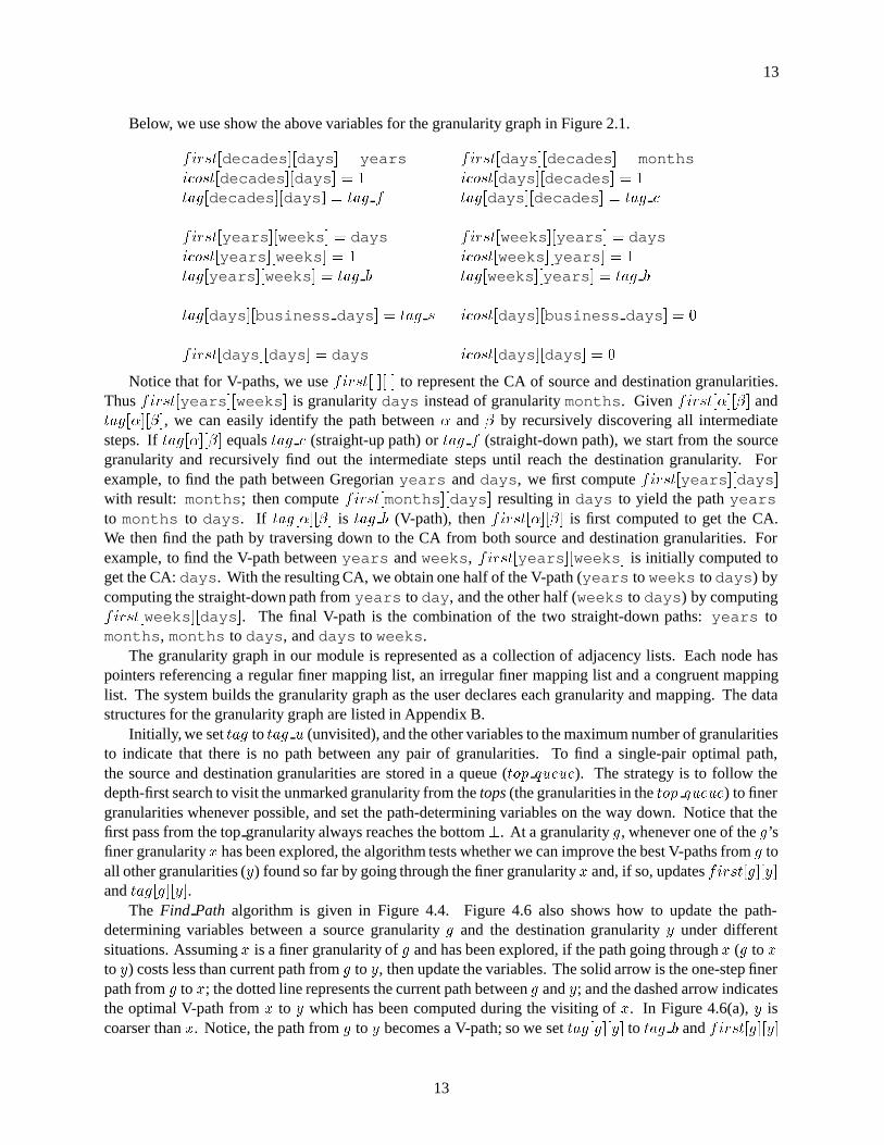
Below, we use show the above variables for the granularity graph in Figure 2.1.

first�decades��days� � years first�days��decades� � monthsicost�decades��days� � � icost�days��decades� � �tag�decades��days] � tag f tag�days��decades� � tag c

first�years��weeks� � days first�weeks��years� � daysicost�years��weeks� � � icost�weeks��years� � �tag�years��weeks� � tag b tag�weeks��years� � tag b

tag�days��business days� � tag s icost�days��business days� � �

first�days��days� � days icost�days��days� � �

Notice that for V-paths, we usefirst� �� � to represent the CA of source and destination granularities.Thusfirst�years��weeks� is granularitydays instead of granularitymonths. Givenfirst������ andtag������, we can easily identify the path between� and� by recursively discovering all intermediatesteps. Iftag������ equalstag c (straight-up path) ortag f (straight-down path), we start from the sourcegranularity and recursively find out the intermediate steps until reach the destination granularity. Forexample, to find the path between Gregorianyears anddays, we first computefirst�years��days�with result: months; then computefirst�months��days� resulting indays to yield the pathyearsto months to days. If tag������ is tag b (V-path), thenfirst������ is first computed to get the CA.We then find the path by traversing down to the CA from both source and destination granularities. Forexample, to find the V-path betweenyears andweeks, first�years��weeks� is initially computed toget the CA:days. With the resulting CA, we obtain one half of the V-path (years toweeks todays) bycomputing the straight-down path fromyears today, and the other half (weeks to days) by computingfirst�weeks��days�. The final V-path is the combination of the two straight-down paths:years tomonths, months to days, anddays to weeks.

The granularity graph in our module is represented as a collection of adjacency lists. Each node haspointers referencing a regular finer mapping list, an irregular finer mapping list and a congruent mappinglist. The system builds the granularity graph as the user declares each granularity and mapping. The datastructures for the granularity graph are listed in Appendix B.

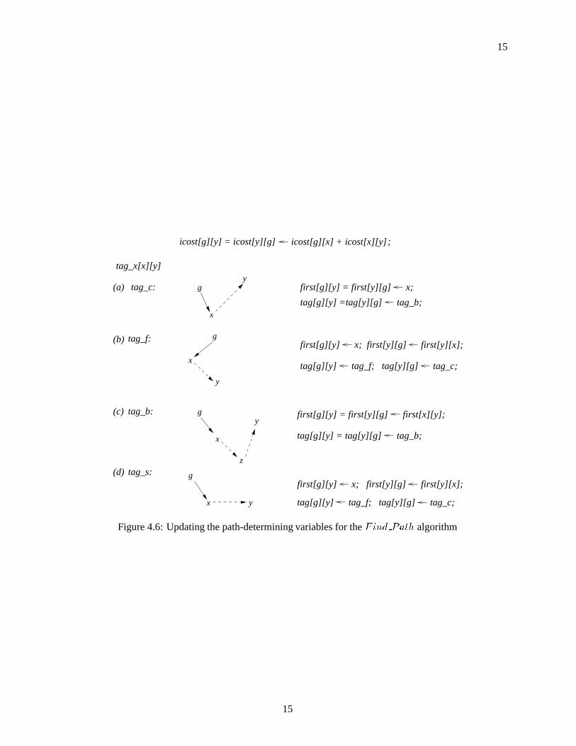
Initially, we settag to tag u (unvisited), and the other variables to the maximum number of granularitiesto indicate that there is no path between any pair of granularities. To find a single-pair optimal path,the source and destination granularities are stored in a queue (top queue). The strategy is to follow thedepth-first search to visit the unmarked granularity from thetops(the granularities in thetop queue) to finergranularities whenever possible, and set the path-determining variables on the way down. Notice that thefirst pass from the topgranularity always reaches the bottom�. At a granularityg, whenever one of theg’sfiner granularityx has been explored, the algorithm tests whether we can improve the best V-paths fromg toall other granularities (y) found so far by going through the finer granularityx and, if so, updatesfirst�g��y�andtag�g��y�.

The Find Path algorithm is given in Figure 4.4. Figure 4.6 also shows how to update the path-determining variables between a source granularityg and the destination granularityy under differentsituations. Assumingx is a finer granularity ofg and has been explored, if the path going throughx (g toxto y) costs less than current path fromg to y, then update the variables. The solid arrow is the one-step finerpath fromg tox; the dotted line represents the current path betweeng andy; and the dashed arrow indicatesthe optimal V-path fromx to y which has been computed during the visiting ofx. In Figure 4.6(a),y iscoarser thanx. Notice, the path fromg to y becomes a V-path; so we settag�g��y� to tag b andfirst�g��y�

13

14

Algorithm 4.3.1 Find Path�G�Input: A granularity graphOutput: first������/* Initialize the variables */for each � and� � G do

assignmax gran num to first������, andicost������;tag������� tag u;

build thetop queue;for each granularityg � top queue do

Do Close�g�;

Figure 4.4: AlgorithmFind Path

Algorithm 4.3.2 Do Close�g�Input: A granularitygOutput: A portion offirst������/* Traverse down the tree by followingg’s finer lists */for each x � g�s finer lists�reg finer list� irreg finer list and congruent list� do

first�g��x�� x� first�x��g�� cg�tag�g��x�� tag f � tag�x��g�� tag c�if x � irreg finer list then icost�g��x�� � else icost�g��x�� ��if tag�x��x� � tag u then Do Close�x��for each y � G and y �� g do

if the cost ofg x y � the cost ofg y

/* Update the variables */Assign new values tofirst�g��y�� first�y��g�� tag�g��y�, andtag�g��y�,and updateicost as shown in Figure 4.6, according to values oftag�x��y�.

Figure 4.5: AlgorithmDo Close

to x. In Figure 4.6(b), y is finer thanx. In Figure 4.6(c), there is a V-path betweenx andy so the updatedpath fromg to x to y is also a V-path. In the final graph 4.6(d), y is congruent withx. The updatedicostis same for all cases and equals the sum of theicosts of the pathsg to x andx to g, where theicost of theone-step finer path (g to x) is 1 for irregular mapping and 0 for regular and congruent mappings.

The algorithm always traverses down following the finer path, this guarantees the V-path constraint.This approach examines all the possible V-paths between a pair of granularities and picks the cheaper patheach time it encounters a new V-path between a pair of granularities, so the final results infirst������ arethe optimal results. In the following we give a formal proof that this algorithm is correct and does indeedcompute the optimal paths.

Lemma 4.3.1 The updated paths represented by the variable first are V-paths.

Proof: Initially, each entry offirst contains the maximum number of granularities to indicate that there is

no path between any pair of granularities. Considering AlgorithmDo Close, the values of thefirst arrayare updated only in following two cases:

1. Traversing down a one-step finer path (fromg to x)

14

15

tag_b;

tag_b;

first[g][y] = first[y][g]

tag[g][y] =tag[y][g]

x;

first[y][x];x; first[y][g]

tag_c;tag_f; tag[y][g]

first[x][y];

x; first[y][g] first[y][x];

tag_c;tag_f; tag[y][g]

icost[g][x] + icost[x][y] ;icost[g][y] = icost[y][g]

first[g][y] = first[y][g]

tag[g][y] = tag[y][g]

first[g][y]

tag[g][y]

first[g][y]

tag[g][y]

x

y(c) g

x y

(d) g

z

x

y(a) g

x

y

(b) g

tag_c:

tag_f:

tag_b:

tag_s:

tag_x[x][y]

Figure 4.6: Updating the path-determining variables for theFind Path algorithm

15

16

first�g��x� � x; first�x��g� � g

The path betweeng andx is obviously a V-path (a straight-up, a straight-down path or a congruentpath).

2. Updating the path betweeng andy through finer granularityx.

This is a recursive graph problem. Due to the existence of an unique bottom in the graph, the first passover the graph always reaches the bottom. The following passes traverse the graph from a granularitydown to the finest unvisited granularity (CA) to build the smallest V-paths, as shown in Figure 4.6(a).The larger V-paths then can be built using the smaller ones as shown in Figure 4.6(c). If granularityy

is finer or congruent withx, then the resulting path is a straight down path fromg to y or a straight uppath fromy to g as in Figure 4.6(b) and (d). Depending on the relationship betweenx andy, whichis built recursively as in Figure 4.6, the new path fromg to y through finer granularityx can only bea straight-down path or a V-path.

We conclude that the updated paths represented by the variablefirst are V-paths. In other words, the finalpaths are V-paths. �

Theorem 4.3.2 If we run AlgorithmFind Path on a pair of granularities, then at termination, the pathsrepresented byfirst�x��y� are the optimal V-paths.

Proof: By Lemma 4.3.1, the paths represented byfirst are V-paths when we run the algorithm. We claim

that our algorithm is basically a top-down, dynamic-programmingalgorithm (namedMemoization) to find the optimal V-path between a pair of granularities. We examine

two key ingredients that must exist to ensure an optimal solution [Cormen et al. 1990].

1. The optimal substructure of the optimal V-path problem.

We say a problem exhibitsoptimal substructureif an optimal solution to the problem contains withinit optimal solutions to subproblems. We use the same notation in AlgorithmDo Closeto illustrate theoptimal substructure in this problem.

Assuming the path (g to x to z to y) is the optimal V-path between granularitiesg andy (here,xis a one-step finer granularity ofg andz is the bottom), then the subpath (x to z to y) must be theoptimal path forx andy. We can proof this by contradiction. If there were a better V-path forx andy, substituting the path ing andy would produce another optimal V-path whose cost was lower thanthe original path: contradiction. Using the same argument, we claim that, for an optimal straight path,assumingg is the coarser granularity, then the subpath (x to y) is the optimal path forx andy. Thus,an optimal solution to an instance of the optimal V-path problem contains within it optimal solutionsto subproblem instances. Note that we always traverse down from the coarser granularity. If we reachbottomz, then the optimal subpath of the straight-path (z to y) is the path: the finer granularity ofyto z.

2. A recursive solution

The second step is to define the value of an optimal solution recursively in terms of an optimalsolutions to subproblems.

Let V icost�g� y� be the number of irregular mappings in the optimal V-path fromg to y, andI icost�g� y� be the number of irregular mappings in straight path from coarser to finer, we candefineV icost�g� y� andI icost�g� y� recursively as follows. Ifg � y, there is no cost. To compute

16

17

V icost�g� y� andI icost�g� y�wheng �� y, we take advantage of the structure of an optimal solutionfrom step 1. Let’s assume that the optimal path forg andy is throughx which is finer than andadjacent tog in the granularity graph. We have

V icost�g� y� � V icost�x� y� � I icost�g� x� , and

I icost�g� y� � I icost�x� y� � I icost�g� x� .

Where,

I icost�g� x� �

�� for irregular mapping

� for regular mapping

The above recursive equation assumes that we know which finer granularity (x) to form the optimalV-path, which we don’t. Sincex is not the only finer granularity ofg and the optimal V-path must beconstructed by going through one of the finer granularities, we need to check them all to find the bestV-path. Thus, the recursive definition for the minimum cost of the optimal V-Path becomes

V icost�g� y� � min

�����

I icost�g� y�I icost�y� g�

minx � g�s finer lists

fV icost�x� y� � I icost�g� x�g

I icost�g� y� �

�� if g finer than y

minx � g�s finer lists

fI icost�x� y� � I icost�g� x�g

Algorithm Find Path is a top-down algorithm based on the above recurrence to compute the optimalV-path. This algorithm is one of the ways to calculate the tables defined above. Combining with Lemma4.3.1, we conclude that the final results infirst array are the optimal V-paths. �

If we search for all top-granularities (granularities with no coarser but some finer or congruent gran-ularities) in the granularity graph and store them instead of the source and destination granularities in thetop queue, the algorithm is extended to solve the all-pairs optimal V-paths for the granularity graph. Thisis easy to see because if we traverse down from top-granularities, each subproblem will be encountered tosolve the optimal V-paths for the entire graph.

What is the running time of the above algorithm? If there arejV j granularities andjEj number ofmappings (edges) in the granularity graphG�V�E�, building the top queue takes timesO�jV j�. Eachgranularity is visited at most once, and procedureDo Close is called exactly once for each granularityin G. During the execution ofDo Close, the loop for the one-step finer granularities ofg is executedjfiner granularities�g�j (the number of one-step finer granularities ofg) times. Since

Pcg�G

jfiner granularities�g�j� O�jEj�,

and there is a testing loop at each granularity, the total running time of AlgorithmFind Path isO�jV j� �O�jV jjEj�, orO�jV jjEj�.

17

Chapter 5

THE Cast OPERATION

TheCast operation is performed to correctly convert time from the source to the destination granularity.Given the optimal path, theCastalgorithm needs to convert a time value from one granularity to anotherin each step of the path. For an irregular mapping step, the algorithm simply invokes the user-definedC functions to convert the granule. For a regular mapping or a congruent mapping, the granule can beconverted by multiplying or dividing by the conversion constant with an anchor adjustment.

For example, to cast an instant, theith granule, from granularity� to granularity�, assuming a regularmapping with conversion constantC, then

Cast�i�� �� �� � i� � C� anchoroffset

We defined in Chapter Two that an anchor is the�th granule of a granularity. In the specification of agranularity graph, the anchor may be defined in terms of a granularity that also needs to be converted. Theuser declares granularities, each with an anchor, the latter in an anchor granularity. As stated in ChapterTwo, we don’t want to require the user to use chronons for the anchor granularity; in other words, we wantto allow non-chronon anchor granularities. For example, a student wishes to design a special calendar forhis academic activities with year origin defined as the first year he was in this department. He knows theorigin is Fall,1995 (the anchor of his special calendar which is defined on the Gregorian years), but mostlikely, he has no idea which chronon that is. We also don’t want to use a same anchor for all granularitiesas we stated in Chapter two.

In this Chapter, we will first describe the problem caused by computing the anchor offset, and thesolution we come up with, then we present the algorithm for theCastoperation and provide the proof ofcorrectness.

5.1 Computing The Anchor Offset

To compute the anchor offset, we need to call theCast algorithm recursively. Unfortunately, this willsometimes cause the algorithm to never halt if the granularity graph declared by the user is not properlyformed. We give the following example to illustrate the termination problem.

Figure 5.1 is a granularity graph with three user-declared granularities (�, �, �) as well as the bottomgranularity (chronons). In this particular example,� and� anchors on chronons and� anchors on�. Notethat� is a coarser granularity than�. When we say�’s anchor is the 4th granule of�, we really mean that�’s anchor is the first chronon in the 4th granule of�. The problem is that the software has no informationabout what�’s anchor is in chronons. Suppose we are to cast theith granule from� to �, we need to knowthe anchor offset of� and�. The following are the steps needed to compute the anchor offset.

18

19

(anchor assumed)

(anchor = 0th granule in Chronons)

(anchor = 5th granule in Chronons)

(anchor = 4th granule in α )

α

β

γ

chronons

Figure 5.1: A granularity graph with nontermination problem

1. We need to calculate anchor of� expressed on granule of�.

2. Given the anchor of� on� (the fourth granule of�), we need to call theCastfunction to cast the 4thgranule from� to �.

Cast�i�� �� �� � i� � C � Cast��� �� ��

The only path we can have in the granularity graph is:� � �

3. Convert the fourth granule in� to granule in�. The result is obviously the 0th granule in�.

4. Then convert the 0th granule in� to �, and we go back to step 1.

This example shows that a user, when defining granularities and anchors, can indeed get into trouble,even when the granularity graph is clearly acyclic. To avoid this problem, we will require that the anchorgranularity be finer than the granularity being defined. This is a reasonable constraint. It will be checkedat DBMS generation time; the module will report an error if this constraint is not satisfied. Given theconstraint, we can prove that theCastalgorithm always terminates. We call the computation of anchoroffset as “anchoring” to differentiate it from the realCastoperation. In the next two sections, we firstpresent theCastalgorithm, then prove the algorithm terminates.

5.2 The Cast Algorithm

Suppose we are to cast a granuleg� from granularity� to � and a granuleg� from granularity� to �.Assuming that� is coarser than�,

Cast�g�� �� �� � bg� � C��� ���c

Cast�g�� �� �� � bg� � C��� ��� � C���c

where,

C��� � �

C��� is the conversion constant from� to�, and�

� is the anchor of� expressed in granule of a finer granularity�.To compute�

� , we use�� , which is�’s anchor defined in the finer granularity�. Then,

19

20

Algorithm 5.2.1 Cast�g� from� to�Input: The granule to be converted (g), the source granularity (from), and

the destination granularity (to).Output: The granule in the destination granularity (result).if from � to then return g;/*find the path between the source and the destination granularities */path� Find Path�from� to�;result� g;while (path is not null)

switch �path�mapping type�case irreg finer mapping:

result� firregular finer mapping�result� path�from� path�to�;case irreg coarser mapping �

result� firregular coarser mapping�result� path�from� path�to�;case reg finer mapping or congruent mapping �

anchor v is the anchor value of (path�from);anchor granularity is the anchor granularity of (path�from);result� bresult � �path�C� �

Cast�anchor v� anchor granularity� path�to�c;case reg coarser mapping �

anchor v is the anchor value of (path�to);anchor granularity is the anchor granularity of (path�to);result� bresult � �path�C� �

Cast�anchor v� anchor granularity� path�from�� path�Cc;path� path�next;

return result;

Figure 5.2: TheCast algorithm

�� � Cast��

� � �� ��

Note that for congruent mapping, either one of the aboveCasts can be used to compute the anchor offset.To perform theCastoperation from a source to a destination granularities, we need to find the optimal

path. The optimal path is stored in a linked list namedpath, of steps. The structure also contains the source(from) and the destination (to) granularities, the mapping types (mapping type), and for regular mapping,the conversion constant (C), for irregular mapping, two pointers pointing to the user-defined C mappingfunctions. Figure 5.2 gives theCastalgorithm.

TheCastalgorithm in Figure 5.2 actually does the path finding and recursive anchoring operation ateach step of the conversion. This is considered inefficient for both the application programs and databasesapplications. In either case, the previously computed optimal V-paths and anchor offsets are cached to avoidthe recomputation. This will be further discussed in next chapter. Recalling that we do not consider therecursive anchor offset computing when we derive theFind Path algorithm, the main reason of ignoringthe anchor offsets is that an anchor offset is computed only when it is first encountered. The computedanchor offset is stored so the value is simply looked up each subsequent time it appears. With the cachingstrategy, the anchor offset computing won’t affect the choice of an optimal V-path.

Notice that in Algorithm 5.2.1, for any determinate instance, theCastalways returns a determinateresult. For any anchored indeterminate instance, the start and the end of the instance are cast separately toget the indeterminate result. Our module provides functions to perform all the standard SQL-92 operations

20

21

for a multicalendar system. The functions are listed in Appendix A.

5.3 Proof Of Termination

The proof of termination involves constructing a bipartite graph for theCastoperation, and using a partialorder to argue the nonexistence of cycles in the graph.

The directed bipartite graph (Gb) is constructed based on the granularity graph (Gg). To distinguish thebipartite graph and the granularity graph, we use the subscriptb to indicate the bipartite graph.

LetGb � �Vb� Eb� Ub� be the bipartite graph. The vertices are partitioned into two disjoint subsets (V b

andUb) such that there is no edge connecting two vertices from the same subset.Vb is a set of anchor offsets needed to be computed in the granularity graphGg. A vertex inVb is denoted

byxy , wherex is a coarser or a congruent granularity ofy inGg and the mapping betweenx andy is either

regular or congruent. Remember there is no need to compute the anchor offset for an irregular mapping.Ub is the other set of vertices in which each vertex represents an one-step mapping in the granularity

graph. A vertex inUb is denoted by�x� y� to indicate the one-step mapping betweenx andy in the granularitygraph.

Eb is a set of directed edges connecting vertices betweenUb andVb. The edges are constructed byfollowing the processes taken to compute an anchor offset. An edge points from a vertexub � �x� y� in thesetUb to a vertexvb � x

y in the setVb if the mapping (x� y) requires computing the anchor offsetxy . Note

that only regular and congruent mappings require to compute the anchor offsets; for an irregular mapping,there is no edge coming out of the node inUb. Given the anchor ofx is in�, the pathp from� toy is neededto compute the anchor offset (x

y). An edge points from an vertexvb � xy in Vb to a vertexub in Ub if the

one-step path inub is contained in the corresponding pathp.Figure 5.3 shows a simple granularity graphGg and the corresponding bipartite graphGb. In the

granularity graph, the anchor of� is in �, the anchors of�, � and are in the chronons� and the anchorof is in . Note that the mapping between� and is an irregular mapping and the mapping between�

and is a congruent mapping. Let’s follow the anchor offset computation of�� to construct the edges for

the bipartite graph. Given�’s anchor in�, the casting path is� �. Since this is a coarser mapping,the required anchor offset is�

� . The anchor of� is defined in�, so to compute�� , the needed path is

� �. Since the path is composed of two steps, there are two edges from�� , pointing to (�� ) and

(� �). Following the anchor offset computation of�� will give us the rest of edges in the bipartite graph.

For this particular example, starting from�� and�

� yields the complete bipartite graph. Note that there isno edge coming out of�

�in Vb and��� �� in Ub. The former is because the anchor offset is given for the

granularity graph; the latter is because the mapping between� and� is irregular. Since theCastalgorithmeffectively follows the edges in the graph, if there is an cycle in the graphGb, theCastalgorithm will notterminate.

To ensure the termination of theCastalgorithm, we add the constraint that the anchor of a granularityshould be defined in a finer granularity. We claim that theCast algorithm will always terminate for agranularity graph satisfying the above constraint. Before we give the formal proof of the claim, let’s definea partial order for the vertices (the one-step paths) in setUb. We use a subscriptp on this partial order todistinguish the coarser relation for the one step paths inU b from the coarser relation for granularities.

21

22

�

�

�

�

�

�

(b)Gb

���

���

���

���

���

����

���I

�

�

�HHHHHHHHHHHHHj

ZZZZZZZZZZZZZ��

�

�XXXXXXXXXXXXz

XXXXXXXXXXXXz

��

���...........

...............

IXXXXXXXXXXXXz

�

(a)Gg

Vb Ub

��� ��

��� ��

��� ��

�����

��� ��

��� ��

Figure 5.3: (a) A simple granularity graph. (b) The corresponding bipartite graph.

Definition 5.3.1 coarser (“�p”) relationshipGiven two vertices in setUb in the bipartite graph:u� � �x�� y�� andu� � �x�� y��,u� �p u� iff

(1) �max�x�� y�� � max�x�� y��� �(2) ��x� � y� � x�� � �y� � x��� �(3) ��x� � y� � y�� � �x� � y���

In above definition,max returns the coarser granularity and chooses an arbitrary granularity if the twogranularities are congruent. The first condition in Definition 5.3.1 is straight forward: the path inU b withthe coarser granularity is the coarser path. The second and third conditions are for special cases: we definea congruent pathu� to be coarser than a path composed of a granularity congruent with granularities inu�and a finer granularity. Applying the definition on Figure 5.3(b), we have

��� �� �p ��� �� �p ��� ��p ��� ��p ���� and

��� ��p ��� �� �p ��� ��p ��� ��p ���� .

Since the definition of the “�p” is based on the relation between granularities, as in the finer relation forgranularities, the “�p” is a partial order. In Figure 5.3(b),��� �� is not coarser than��� ��, and��� �� is notcoarser than��� ��. The “�p” also has the following two properties, which follow from its definition:

� Transitivity: if ui �p uj anduj �p uk thenui �p uk .

� Inreflexivity: ui ��p ui .

22

23

With Definition 5.3.1 and the assumption about the finer anchor granularity, we argue that starting fromany vertex in theGp built on a granularity graph satisfying the constraint about the finer anchor granularity,and following the direction of edges to compute an anchor offset, the encountered vertices in the setU arein descending order with respect to the “�p” relation.

Lemma 5.3.2 Given a granularity graph, if the anchor of each granularity is defined in a finer granularity,then following an arbitrary edge in the corresponding bipartite graph, for any two consecutive verticesu i

andui�� in Ub, we haveui �p ui�� :

Proof: Let ui be an arbitrary one-step path (�� �) in Ub and�’s anchor is in�. Assuming� is finer than�,

an edge in the bipartite graph points fromui to �� . The outward edges from�

� should point to each stepof the pathp from � to� in order to compute the anchor offset. The pathp must be either a straight-up path,a straight-down path or a V shape path in the granularity graph. Letui�� be any consecutive vertex in thebipartite graph, then the pathp can be expressed as� � � � �.

1. For a straight-up path, due to the transitivity of granularities, we have

� � � � � � � .

Along with the assumption that� � �, it’s straight forward to see that all granularities in the pathp

is finer than�. By Definition 5.3.1 (1), we prove thatui �p ui�� .

2. For a straight-down path,

� � � � � � � .

Given� � � from the constraint about the finer anchor granularity, as in step 1, all granularities inthe pathp are finer than� resulting inui � ui�� .

3. For a V shape path, theCA is finer than� and� by theCA definition. From step 1 and step 2, weimmediately haveui �p ui�� .

If � is congruent with�, because of the assumption of the finer anchor granularity, the pathp from � to� can only be a straight-up path or a V-path. Applying step 1 and step 3, and plus Definition 5.3.1 (2) and(3), we also findui �p ui��. Combining the all steps, we have proved the Lemma. �

Now we can further prove that given the constraint, theCastalgorithm terminates.

Theorem 5.3.3 Given a granularity graph, if the anchor of each granularity is defined in a finer granularity, then the Cast algorithm on any pair of granularities always terminates.

Proof: This is proved by contradiction.

Suppose the algorithm does not terminate. Since each step of theCastalgorithm traverses an edge ofGb, and since there are finite number of nodes in this graph, there must be a cycle in the bipartite graphGb.The cycle contains two verticesui anduj in Ub such that

ui � � � uj � � � ui .Then according to Lemma 5.3.2 and the transitivity of “�p”, we haveui �p ui .

This is in contradiction with the inreflexivity of “�p”, so we have proved Theorem 5.3.3. �

23

Chapter 6

PERFORMANCE

Performance is an important issue. Our goal is to provide a package to support the multiple time granularitieswithin both application programs and databases. A scalable solution, capable of handling hundreds ofgranularities, is desired. We use several strategies to improve the performance.

The first strategy is to compose the path for regular mappings and congruent mappings with the sameanchor. We defineacost as the cost of the anchor adjustments in the path. For V-paths between a pairof granularities, theicost (the number of irregular mappings) is the major factor to choose which path isbetter. If two granularities have the same anchor and the same anchor offset, then theacost of these twogranularities is zero. In the case of the sameicost, the path with smalleracost will be selected. Theacostis also used to improve the performance further. For a straight-line path (either finer or coarser path), iftheacost is zero in each step, and there is no irregular mapping in the path, then the path can be combinedinto a single step with a new conversion constant to reduce the mappings. For example, in Figure 2.1,the mappings fromdays hours minutes can be combined asdays minutes with a newconversion constant 1440.

Since the number of the anchor offsets needed to be computed in a granularity graph is a fixed number,the number of edges, we use a lazy caching strategy to improve the performance. An anchor offset iscomputed on demand and stored in the front of the cache, which is a linked list. Each subsequent time thisanchor offset is encountered, the value in the list is used and the anchor offset is moved to the front of thelist. When the cache is full, the values at the back of the list are freed to give space for the newly computedanchor offsets. We envision that if there aren’t a great many edges, the cache can be made large enough tohold all anchores.

The performance of computing the optimal V-paths is more complicated. We emphasize that our moduleis designed to support both application programs and databases. As we stated in Chapter 4.3, for databaseapplications, during the graph specification the optimal V-paths computation can be very slow, but theCastmust be fast at query-time. If the set of granularities is small, the optimal V-path between any two pair ofgranularities can be determined at DBMS generation time, as the declaration is done. However, as thereareO�jV j�� optimal V-paths in a given granularity graphG�V�E�, for many application programs that castand scale between a small subset of granularities, computing all optimal V-paths is overkill. Our solutionis to allow precomputation optionally, as a separate user command. This would be appropriate for databaseapplications. For application programs, we use the lazy caching approach: the optimal V-path is calculatedon demand and cached after the computation.

To quantify the actual cost of computing an optimal V-path, we ran a series of tests on the multicalendargranularity graph shown in Figure 2.1, with 18 granularities and 20 edges. We start with a sequence of pairsof randomly selected granularities. As the length of the sequence increases, we expect that the average costper optimal V-paths (termed theV-cost) will drop for the lazy caching approach. We then vary the degree

24

25

of randomness and the cache size to determine the effect of the lazy caching strategy. To precisely measurethe V-cost, we ran the tests on a DEC 2000/233 workstation (with an Alpha 21064 processor running at233MHz) and use the atom tool [SE94] to measure the number of cycles spent in computing an optimal path.Each test is repeated 50 times (each time with a random sequence of pairs) to get the average results. TheV-cost is computed by dividing the total cost of searching the paths by��� sequence length. The followingis the parameters used in the tests:

AlgorithmsThe algorithms used to compute the optimal V-paths:

DP-ALLThe dynamic programming approach (DP), using Algorithm 4.3.1 toprecompute the variablefirst for the all-pairs (ALL) optimal V-paths.

DP-SThe dynamic programming approach (DP), using Algorithm 4.3.1 to compute the variablefirst as needed for a single (S) pair of granularities .

EDSP-SThe extendedDag-Shortest-PathsAlgorithm (EDSP), to compute the optimal V-path asneeded for a single pair (S) of granularities without caching.

EDSP-SCThe extendedDag-Shortest-PathsAlgorithm (EDSP), to compute the optimal V-path asneeded for a single pair (S) of granularities with the lazy caching strategy (C).

Sequence LengthThe length of the call sequences with values 1, 2, 4, 8, 16, 32, 64, 128 and 256.

Cache SizeThe cache size for EDSP-SC with values 1KB, 2KB, 3KB, 4KB, 5KB, 6KB, 7KB and 8KB.

Degree of RandomnessThe number of the unique pairs of granularities needed to compute the optimalV-paths, with values 1, 2, 4, 8, 16, 32, 64, 128 and 256. Forn unique pairs of granularities, thepairs are generated randomly, then pairs are randomly chosen to form a series of calls. A value of 1specifies all pairs are identical; a values of 256 results in a totally random sequence of pairs.

Figure 6.1 shows the V-cost versus sequence length with randomly generated sequences for differentalgorithms. We choose the cache size 1KB for EDSP-SC to match the size of the variables (first, tag andcost) in Algorithms DP-ALL and DP-S. For DP-ALL, precomputing thefirst variable costs 156555 cycles.Figure 6.1 shows the V-cost with the precomputation and without the precomputation. As one would expect,the V-cost for EDSP-S (16684 cycles) is much higher (8 times higher) than that for DP-ALL (2331 cycles notincluding the precomputation). As shown in the graph, for EDSP-SC, the 1KB cache has no effect on the costbecause of the randomly generated sequences. Figure 6.2 is a log scaled version of Figure 6.1. We observethat for shorter sequences (sequence length� ), the V-costs for DP-ALL (including the precomputation)and DP-S are higher than those for EDSP-SC and EDSP-S. This makes sense — Algorithm DP-ALL andDP-S use a dynamic programming approach, thus computing the optimal V-paths for subproblems. Forlonger sequences, the V-costs for DP-ALL and DP-S reduce quickly below the cost for EDSP-S since thepreviously computed optimal V-paths are simply looked up in thefirst variable. Note that, for longersequences, the cost for DP-ALL drops even faster than that for DP-S.

Figure 6.3 gives the result for different degrees of randomness for the DP-S approach. The curvesshow that a lower degree of randomness yields a smaller V-cost. The interesting point is that the V-costfor different randomness are not dramatically different. At longer sequences, the costs are quite similar fordifferent randomness.

Figure 6.4 and Figure 6.5 show the performance for Algorithm EDSP-SC. We wish to determinate theright cache size for different randomness. In Figure 6.4, we measure the V-cost versus sequence length witha fixed degree of randomness of 8 for different cache sizes. As shown in the figure, clearly, the 2KB cache issufficient for the sequences with 8 unique pairs. The V-cost drops rapidly as the sequence length increases.

25

26

0

5000

10000

15000

20000

25000

30000

35000

40000

45000

50000

0 50 100 150 200 250 300

Ave

rage

tim

e pe

r op

timal

V-p

ath

(cyc

les)

Sequence Length

DP-ALL without precomputationDP-ALL with precomputation

DP-SEDSP-SC with 1KB cache

EDSP-S

Figure 6.1: The V-cost versus Sequence Length.

2000

5000

10000

20000

30000

40000

5000060000700008000090000

100000

150000

1 2 4 8 16 32 64 128 256

Ave

rage

tim

e (lo

g) p

er o

ptim

al V

-pat

h (c

ycle

s)

Sequence Length (log)

DP-ALL without precomputationDP-ALL with precomputation

DP-SEDSP-S

Figure 6.2: The V-cost versus Sequence Length.

26

27

0

5000

10000

15000

20000

25000

30000

35000

40000

45000

1 2 4 8 16 32 64 128 256

Ave

rage

tim

e pe

r op

timal

V-p

ath

(cyc

les)

Sequence Length (log)

Randomness=1Randomness=2Randomness=4Randomness=8

Randomness=16Randomness=32Randomness=64

Randomness=128Randomness=256

Figure 6.3: The V-cost versus Sequence Length for DP-S.

For sequences longer than 64 pairs, the V-cost drops below that (2331 cycles) for DP-ALL in Figure 6.1,which shows that for a degree of randomness of 8 and a sequence length� �, EDSP-SC provides the bestperformance.

To further evaluate the effect of the lazy caching strategy, we ran further tests with different randomnessfor EDSP-SC. Figure 6.5 shows the results. This figure indicates which cache size is sufficient for differentdegree of randomness. For example, 3KB is enough for Randomness=16 and 5KB for Randomness=32.Surprisingly, we find that with 3KB cache, Algorithm EDSP-SC can achieve the best performance (the costper optimal V-path is less than 500 cycles comparing with 2231 cycles for DP-ALL) for sequences up to 16unique pairs.

These analysis shows that different algorithms do affect the cost of theCastoperations. Althoughthe tests ware done only on one granularity graph, that of Figure 2.1, the results suggest that for a user,performing theCasts with higher degree of randomness and shorter sequence length, EDSP-S works fine;for lower degree of randomness (� ��), EDSP-SC with small cache size (about 3KB for this particulargraph) provides surprisingly good results; for higher degree of randomness and longer sequence length,precomputation (DP-ALL and DP-S) are the best choices.

27

28

0

2000

4000

6000

8000

10000

12000

8 16 32 64 128 256

Ave

rage

tim

e pe

r op

timal

V-p

ath

(cyc

les)

Sequence Length (log)

cache=1KBcache=2KBcache=3KBcache=4KB

Figure 6.4: The V-cost versus Sequence Length with Randomness=8 for EDSP-SC.

0

2000

4000

6000

8000

10000

12000

14000

16000

18000

1 2 4 8 16 32 64 128 256

Ave

rage

tim

e pe

r op

timal

V-p

ath

(cyc

les)

Degree of Randomness

cache=1KBcache=2KBcache=3KBcache=4KBcache=5KBcache=6KBcache=7KBcache=8KB

Figure 6.5: The V-cost versus Degree of Randomness with Sequence Length=256 for EDSP-SC.

28

Chapter 7

SUMMARY

This thesis involves elaborating a software architecture for supporting multiple time granularities within anapplication program or a database. First, we described a granularity as partitioning of the time-line, andthe mapping relationship for a pair of granularities, which may be either a regular mapping, an irregularmapping or a congruent mapping. We showed how to weave granularities from different calendars into asingle granularity graph. In Chapter Three we also pointed out the three requirements for a properly formedgranularity graph. When the graph is declared, the module will check the graph and report any errors. Wedescribed why the V-paths are the correct paths to perform theCastoperation and proved that all V-pathsyield the same result. We then extended the shortest path algorithm to compute the optimal path for a singlepair of granularities and also presented an dynamic programming algorithm to solve the all-pairs optimalV-paths. We pointed out the nontermination problem in the computation of anchor offset and proved thatgiven a granularity graph, if the anchor of each granularity is defined in a finer granularity, then theCastalgorithm on any pair of granularities always terminates. Chapter Five gave the correctCastalgorithm forcasting the anchored time values. Finally, we presented our strategies to improve the performance. Weemphasized that our module is to support both application programs and database management systems andwe also described the different performance requirement for application programs and DBMSs. The lazycaching strategy is recommended to avoid computing previously computed results. The external moduleinterface is listed in Appendix A. This work will serve as an important part of a comprehensive library,supporting both temporal DBMSs and application programs that handle time values.

There are some future work can be done. First, this thesis assumes that the costs for all irregularmappings are the same by assigning a cost of 1 to all edges. Such an approach has a drawback, however. Itdoes not distinguishthe edges with different execution time, which may affect the computation of the optimalpath. If we know the execution costs of irregular mappings, our module interface can easily be extended toprovide potentially faster V-paths. Second, this thesis does not deal withintervals, i.e., unanchored durationsof time. An interval is an amount of time with a known length but no specific starting or ending instants[Dyreson & Snodgrass 1994A]. For example, an interval two months has a duration of two months, but canbe any block of two consecutive months, which could be a wide ranges of days due to the irregular mappingbetween months and days. Given leap granules and various arbitrary aspects of calendars, computing theduration of an interval in a finer granularity is generally complex. The computation involves checking theevery possible duration in the entire time line of the interval granularity, which is practically impossible.Therefore, how to compute intervals in the granule operations is still an open question in temporal databases.

29

Appendix A

THE EXTERNAL INTERFACE

/* The internal timestamp with maximum 96 bits. */typedef int polymorphic int;

/* The mappings types */ typedef enum freg finer,reg coarser,conguent,irreg finer,irreg coarser

g mapping type;

/* The possible error types */typedef enum f

gran OK,gran not found,gran other not found,gran exists,gran result not available,gran overflow,gran cross calender operators,gran too many granularities,gran lattice error

g gran error type;

/* granularity is a global notion. Each is supplied by a calendar. */typedef unsigned char granularity;

/** Each calendar also has, known to it, local identifiers, which are* integers, of the granularities it supports. When any of the mapping* or other calendar-specific functions are called, the granularities* are always referred to by their local identifiers, which should be* known to the calendar.*//** There is a distinguished granularity, 0, with anchor 0, in relation* to which all other granularities are defined. The distinguished* granularity is the base-line second.*/static const granularity second granularity=0;

extern granularity gran default granularity;

30

31

/* USED FOR INITIALIZATION *//** Routine: declare granularity** Description: Declare a granularity, and associate an anchor with it.** Arguments: id -- (IN): granularity being associated with the anchor* calendar id -- (IN): identifies the calendar that* supports this granularity* local id -- (IN): the local identifier for the* granularity, within the calendar* anchor -- (IN): position of anchor* anchor gran -- (IN): the granularity of the anchor** Return Value: Error Code** Errors: gran exists** Side Effects: Granularity id, if not previously declared,* is now defined.*/gran error type declare granularity(granularity id, int calendar id,

int local id, polymorphic int anchor, granularity anchor gran);

/** Routine: declare congruent** Description: Declare two granularities to be identical partitionings* of the underlying time line (with possibly different* anchors). This relationship is reflexive, symmetric* and transitive.** Arguments: one -- (IN): one of the congruent granularities* two -- (IN): the other congruent granularity** Return Value: Error Code** Errors: gran not found: if one not found* gran other not found: if two not found** Side Effects: The two granularities, and any previously congruent* granularities, and considered to be congruent.*/gran error type declare congruent (granularity one, granularity two);

/** Routine: declare irregular mapping** Description: Declare an irregular mapping from one granularity to* another. The mapping consists of three functions* that are available for converting a value in one* granularity to a value in a different granularity.* Mappings are allowed only between granularities* supported by the same calendar.** Arguments: from -- (IN): the source granularity* to -- (IN): the destination granularity* cast -- (IN): user-defined function that yields the* closest determinate value in the destination* granularity where cast has the following* parameters:

31

32

* from -- (IN): local id of the source granularity* to -- (IN): local id of the destination granularity* this lower -- (IN): value to be converted* result -- (OUT): value in the to granularity* and returns an error code (gran not found or* gran other not found)* scale determinate -- (IN): user-defined function that* yields a possibly indeterminate value (in the* destination granularity) of a determinate value* in the source granularity where scale determinate* has the following parameters.* from -- (IN): local id of the source granularity* to -- (IN): local id of the destination granularity* this lower -- (IN): value to be converted* result lower -- (OUT): lower support in the to* granularity* result upper -- (OUT): upper support in the to* granularity* and returns an error code (gran not found or* gran other not found)* scale indeterminate -- (IN): function that yields a* possibly indeterminate value (in the destination* granularity) of an indeterminate value in the source* granularity where scale indeterminate has the* following parameters* from -- (IN): local id of the source granularity* to -- (IN): local id of the destination granularity* this lower -- (IN): value to be converted* this upper -- (IN): value to be converted* result lower -- (OUT): lower support in the to* granularity* result upper -- (OUT): upper in the to granularity* and returns an error code (gran not found* or gran other not found)** Return Value: Error Code** Errors: gran not found: if from not found* gran other not found: if to not found** Side Effects: Mapping is recorded for use in conversion operations.*/gran error type declare irregular mapping(granularity from,

granularity to,gran error type (*cast finer)(),gran error type (*cast coarser)(),gran error type (*scale determinate)(),gran error type (*scale indeterminate)());

/* * Routine: declare regular mapping** Description: Declare an irregular mapping from one granularity to* another. A regular mapping is simply an integral* to conversion. An example is from hours to minutes* by multiplying by 60. An anchor adjustment may also* be required. Regular mappings can be defined between* granularities supported by different calendars.** Arguments: from -- (IN): the source (coarser) granularity* to -- (IN): the target (finer) granularity* conversion -- (IN): the multiplicative conversion factor** Return Value: Error Code

32

33

** Errors: gran not found: if from not found* gran other not found: if to not found** Side Effects: Mapping is recorded for use in conversion operations.*/gran error type declare regular mapping(granularity from,

granularity to, int conversion);

/** Routine: declare e plus s** Description: Declare a function to do this arithmetic operation* in the indicated span granularity.** Arguments: s gran -- (IN): granularity of the event* e plus s -- (IN): function which can perform the operation* where e plus s has the following parameters* e -- (IN): source event* e gran -- (IN): local granularity of the event* s -- (IN): source span* s gran -- (IN): local granularity of the span* result -- (OUT): the event resulting from the,* addition in the e gran* and returns an error code (gran not found or* gran other not found)** Return Value: Error Code** Errors: gran not found** Side Effects: The function pointer is stored, or overwritten if* previously present, for later use.****gran error type declare e plus s(granularity s gran,* gran error type (*e plus s)(polymorphic int e,* granularity e gran, polymorphic int s,* polymorphic int* result));*/gran error type declare e plus s(granularity s gran,

gran error type (*e plus s)());

/** Routine: declare s plus e** Description: Declare a function to do this arithmetic operation in* the indicated span granularity.** Arguments: s gran -- (IN): granularity of the span* s plus e -- (IN): function which can perform the operation* where s plus e has the following parameters* s -- (IN): source span* e -- (IN): source event* e gran -- (IN): local granularity of the span* result -- (OUT): the event resulting from the* addition in the s gran* and returns an error code (gran not found)** Return Value: Error Code*

33

34

* Errors: gran not found** Side Effects: The function pointer is stored, or overwritten if* previously present, for later user**gran error type declare s plus e(granularity s gran,* gran error type (*s plus e)(polymorphic int s,* polymorphic int e, granularity e gran,* polymorphic int *result));*/gran error type declare s plus e(granularity s gran,

gran error type (*s plus e)());

/** Routine: declare e minus e** Description: Declare a function to do this arithmetic operation with* the indicated result granularity.** Arguments: result gran -- (IN): desired granularity of the result* e minus e -- (IN): function which can perform the operation* where e minus e has the following parameters:* left -- (IN): source event* left gran -- (IN): local granularity of left* right -- (IN): other source event* right gran -- (IN): local granularity of right* result -- (OUT): the span resulting from the* subtraction, in the result gran* and returns an error code (gran not found or* gran other not found)** Return Value: Error Code** Errors: gran not found** Side Effects: The function pointer is stored, or overwritten if* previously present, for later use.**gran error type declare e minus e(granularity result gran,* gran error type (*e minus e)(polymorphic int left,* granularity left gran,* polymorphic int right,* granularity right gran,* int *result));*/gran error type declare e minus e(granularity result gran,

gran error type (*e minus e)());

/** Routine: declare extract** Description: Declare an extraction function requesting a specified* granularity** Arguments: right gran -- (IN): the specified granularity* extract -- (IN): a function which performs the requested* operation.* where extract has the following parameters:* right gran--(IN): the specified granularity* right -- (IN): an event* left gran -- (IN): the requested granularity* result -- (OUT): the value of the requested

34

35

* granularity* and returns an error code (gran not found, gran overflow)** Return Value: Error Code** Errors: gran not found** Side Effects: None.**gran error type declare extract(granularity right gran,* gran error type (*extract)(granularity right gran,* polymorphic int right,* granularity left gran,* int *result) );*/gran error type declare extract(granularity right gran,

gran error type (*extract)());

/** Routine: extract** Description: Extracts the indicated component of the argument event* or span. As an example, extracting the year from the* event "April 19, 1955" yields 1955. Extracting the* month yields 4, and extracting the day yields 19.* Of course, the specific values returned are* calendar-dependent.** Arguments: left gran -- (IN): the granularity to be extracted* right -- (IN): an event or span, from which the value* is to be extracted* right gran -- (IN): the granularity of right* result -- (OUT)** Return Value: Error Code** Errors: gran not found* gran other not found* gran cross calender operators* gran overflow -- the integer returned is too big to* fit in an int** Side Effects: A calendar supplied function is called.*/gran error type extract(granularity left gran, polymorphic int right,

granularity right gran, int *result);

/** Routine: scale determinate** Description: Yields a possibly indeterminate value (in the* destination granularity) of a determinate value* in the source granularity** Arguments: original -- (IN): value to be converted* from -- (IN): the source granularity* to -- (IN): the target granularity* result lower -- (OUT): lower support in the to* granularity* result upper -- (OUT): upper support in the to* granularity*

35

36

* Return Value: Error Code** Errors: gran not found: if from not found* gran other not found: if to not found** Side Effects: One or more calendar supplied functions may be called.*/gran error type scale determinate(polymorphic int original,

granularity from, granularity to,polymorphic int* result lower,polymorphic int* result upper);

/** Routine: scale indeterminate** Description: Yields an indeterminate value (in the destination* granularity) of a determinate value in the source* granularity.** Arguments: this lower -- (IN): lower support of value to be converted* this upper -- (IN): upper support of value to be converted* from -- (IN): the source granularity* to -- (IN): the target granularity* result lower -- (OUT): lower support in the to* granularity* result upper -- (OUT): upper support in the to* granularity** Return Value: Error Code** Errors: gran not found: if from not found* gran other not found: if to not found** Side Effects: One or more calendar supplied functions may be called.*/gran error type scale indeterminate(polymorphic int this lower,

polymorphic int this upper, granularity from,granularity to, polymorphic int *result lower,polymorphic int* result upper);

/** Routine: cast** Description: Yields the first determinate value in the destination* granularity of a value, either determinate, or lower* support if indeterminate** Arguments: this lower -- (IN): input event* from -- (IN): source granularity* to -- (IN): target granularity* result -- (IN): ** Return Value: Error Code** Errors: gran not found: if from not found* gran other not found: if to not found** Side Effects: A calendar supplied function is called.*/gran error type cast(polymorphic int this lower, granularity from,

granularity to, polymorphic int* result);

36

37

/** Routine: e plus s** Description: Adds an event and a span, of mixed granularities,* yielding an event.** Arguments: e gran-- (IN): granularity of the event* e -- (IN): the source event* s gran -- (IN): granularity of the span* s -- (IN): the source span* result -- (OUT): The result is in e gran** Return Value: Error Code** Errors: gran not found: if e gran not found* gran other not found: if s gran not found* gran cross calender operators** Side Effects: A calendar supplied function is called.*/gran error type e plus s(granularity e gran, polymorphic int e,

granularity s gran, polymorphic int s,polymorphic int* result);

/** Routine: s plus e** Description: Adds an event and a span, of mixed granularities,* 3.2cmyielding an event.** Arguments: s gran -- (IN): the granularity of the span* s -- (IN): the source span* e gran -- (IN): the granularity of the event* e -- (IN): the source event* result -- (OUT): in the s gran granularity** Return Value: Error Code** Errors: gran not found: if s gran not found* gran other not found: if e gran not found* gran cross calender operators** Side Effects: A calendar supplied function is called.*/gran error type s plus e(granularity s gran, polymorphic int s,

granularity e gran, polymorphic int e,polymorphic int* result);

/** Routine: e minus e** Description: Subtracts two events, in mixed granularities,* yielding a span, in a specified granularity.** Arguments: left gran -- (IN): granularity of left* left -- (IN): one of the source events* right gran -- (IN): granularity of right* right -- (IN): the other of the source events* result gran -- (IN): the desired resulting granularity* result -- (OUT): ** Return Value: Error Code*

37

38

* Errors: gran not found: if from not found* gran other not found: if to not found* gran cross calender operators** Side Effects: A calendar supplied function is called.*/gran error type e minus e(granularity left gran,

polymorphic int left, granularity right gran,polymorphic int right, granularity result gran,polymorphic int* result);

38

Appendix B

THE INTERNAL DATA STRUCTURE

/* The linked-list structure for regular mappings. It contains the* destination granularity, the conversion constant and a pointer* referencing the next finer mapping.*/typedef struct reg map list struct f

int conversion;granularity destination;struct reg map list struct *next ptr;

g reg map list type;

/* The linked-list structure for irregular mappings. It contains the* destination granulairty, the irregular mapping funtions and a* pointer referencing the next irregular mapping.*/typedef struct irreg map list struct f

granularity destination ;gran error type (*cast)(); /*user-defined function*/gran error type (*scale det)(); /*user-defined function*/gran error type (*scale indet)(); /*user-defined function*/struct irreg map list struct *next ptr;

g irreg map list type;

/* The structure for the granularity graph. It contains the* user id given by the user, the internal id: local id,* the calender id which the granularity belongs to, the* anchor and the anchor granularity. It also contains pointers* referencing the regular mapping list, the irregular mapping* list and thecongruent mapping list.*/typedef struct gran lattice struct f

granularity user id;int calender id;int local id;polymorphic int anchor;granularity anchor gran;reg map list type *reg map coarser list;reg map list type *reg map finer list;reg map list type *cong map list;irreg map list type *irreg map coarser list;irreg map list type *irreg map finer list;

g gran lattice type;

/* The structure for the optimal path. It contains the source* granularity, the destination granularity, the mapping type,

39

40

* the conversion constant for the regular mapping and mapping* functions for irregular mappings. It also has a pointer* referencing the next step in the path.*/typedef struct super path struct f

granularity from;granularity to;double conversion;mapping type map type; /*mapping type*/gran error type (*cast)();gran error type (*scale det)();gran error type (*scale indet)();struct super path struct *next ptr;

g super path type;typedef super path type *super path type ptr;

40

Bibliography

[Anderson 1982] Anderson, T. L., “Modeling Events and Processes at the Conceptual Level,” inPro-ceedings of the Second International Conference on Databases: Improving Usability Responsiveness.Ed. P. Scheuermann. Jerusalem, Israel: Academic Press, June 1982, pp. 273–297.

[Cattell 1994] Cattell, R. G. G., “The Object Database Standard: ODMG-93” San Mateo, CA: MorganKaufmann Publishers, Inc., 1994.

[Clifford & Rao 1987] Clifford, J. and A. Rao., “A Simple, General Structure for Temporal Domains,” inProceedings of the Conference on Temporal Aspects in Information Systems. AFCET. France: May1987, pp. 247–265.

[Cormen et al. 1990] Cormen, T. H. and R. Rivest, “Introduction To Algorithms” London, England: TheMIT Press, 1990.

[Dershowitz et al. 1990] DershowitzN. and E. Reingold, “Calendrical calculations,” inSoftware—Practiceand Experience, 20, No. 9(1990), pp. 899–928.

[Dyreson & Snodgrass 1993] Dyreson, C. E. and R. Snodgrass, “Valid-time Indeterminancy,” inProceed-ings of the International Conference on Data Engineering. 1993, pp. 335–343.

[Dyreson & Snodgrass 1994A] Dyreson, C. E. and R. Snodgrass, “Temporal Granularity and Indetermi-nacy: Two Sides of the Same Coin.” Technical Report TR94-06. Computer Science Department,University of Arizona. Feb., 1994.

[Dyreson & Snodgrass 1994B] Dyreson, C. E. and R. Snodgrass, “Efficient Timestamp Input and Output,”in Software-Practice and Experience, 24, No. 1(1994), pp. 80–109.

[Kraus et al. 1996] Kraus, S., Y. Sagiv and V. Subrahmanian, “Representing and Integrating MultipleCalendars.” Submitted for publication.

[Melton & Simon 1993] Melton, J. and A. R. Simon. “Understanding the New SQL: A Complete Guide”San Mateo, CA: Morgan Kaufmann Publishers, Inc., 1993.

[Reingold et al. 1993] Reingold E. M., N. Dershowitz and S. Clamen, “Calendrical Calculations, II: ThreeHistorical Calendars,” inSoftware—Practice and Experience, 23, No. 4(1993), pp. 383–404.

[Snodgrass 1995] Snodgrass, R., “The TSQL2 Temporal Query Language” Dordrecht, The Netherlands:Kluwer Academic Publishers, 1995.

[SE94] Srivastava, A. and A. Eustace, ATOM: A System for Build Customized Program Analysis Tools.In Proceedings of the ACM SIGPLAN ’94 Conference on programming Language Design and Imple-mentation, pp. 196–205, June 1994

41

42

[Vinogradov et al. 1988] Vinogradov, I. M., “Encyclopaedia Of Mathematics” Dordrecht, The Netherlands:Kluwer Academic Publishers, 1988, V2, pp. 255.

[Wang et al. 1993] Wang, X., S. Jajodia and V. Subrahmanian, “Temporal Modules: An Approach TowardTemporal Databases,” inProceedings of the ACM SIGMOD InternationalConferenceon Manegementof Data. 1993, pp. 227–236.

[Wiederhold et al. 1991] Wiederhold, G., S. Jajodia and W. Litwin., “Dealing with Granularity of Time inTemporal Databases,” inProceedings Nordic Conference on Advanced Information Systems Engi-neering. Trondheim, Norway: May 1991.

42