Efficient Diversification

Risk Premiums and Risk Aversion

• Degree to which investors are unwilling to accept uncertainty– Risk aversion

• If T-Bill denotes the risk-free rate, rf, and variance, σp

2 , denotes volatility of the portfolio returns then:

The risk premium of a portfolio is:

Risk Premiums and Risk Aversion

• To quantify the degree of risk aversion with parameter A:

» Or:

The Sharpe (Reward-to-Volatility) Measure

ASSET ALLOCATION ACROSS RISKY AND RISK-FREE

PORTFOLIOS

• Possible to split investment funds between safe and risky assets

• Risk free asset: T-bills• Risky asset: stock (or a portfolio)

Allocating Capital

Allocating Capital

• Issues– Examine risk vs return tradeoff– Demonstrate how different degrees of

risk aversion will affect allocations between risky and risk free assets

The Risky Asset: Example

Total portfolio value = $300,000

Risk-free value = $90,000

Risky (Vanguard and Fidelity) = $210,000

Vanguard (V) = 54%

Fidelity (F) = 46%

The Risky Asset: Example

Vanguard 113,400/300,000 = 0.378

Fidelity 96,600/300,000 = 0.322

Portfolio P 210,000/300,000 = 0.700

Risk-Free Assets F 90,000/300,000 = 0.300

Portfolio C 300,000/300,000 = 1.000

rf = 7%rf = 7% srf = 0%srf = 0%

E(rp) = 15%E(rp) = 15% sp = 22%sp = 22%

y = % in py = % in p (1-y) = % in rf(1-y) = % in rf

Calculating the Expected Return: Example

E(rc) = yE(rp) + (1 - y)rfE(rc) = yE(rp) + (1 - y)rf

rc = complete or combined portfoliorc = complete or combined portfolio

For example, y = .75For example, y = .75E(rc) = .75(.15) + .25(.07)E(rc) = .75(.15) + .25(.07)

= .13 or 13%= .13 or 13%

Expected Returns for Combinations

ppcc ==

SinceSince rfrf

yy

Variance on the Possible Combined Portfolios

= 0, then= 0, thenss

ssss

cc= .75(.22) = .165 or 16.5%= .75(.22) = .165 or 16.5%

If y = .75, thenIf y = .75, then

cc= 1(.22) = .22 or 22%= 1(.22) = .22 or 22%

If y = 1If y = 1

cc= 0(.22) = .00 or 0%= 0(.22) = .00 or 0%

If y = 0If y = 0

Combinations Without Leverage

ss

ss

ss

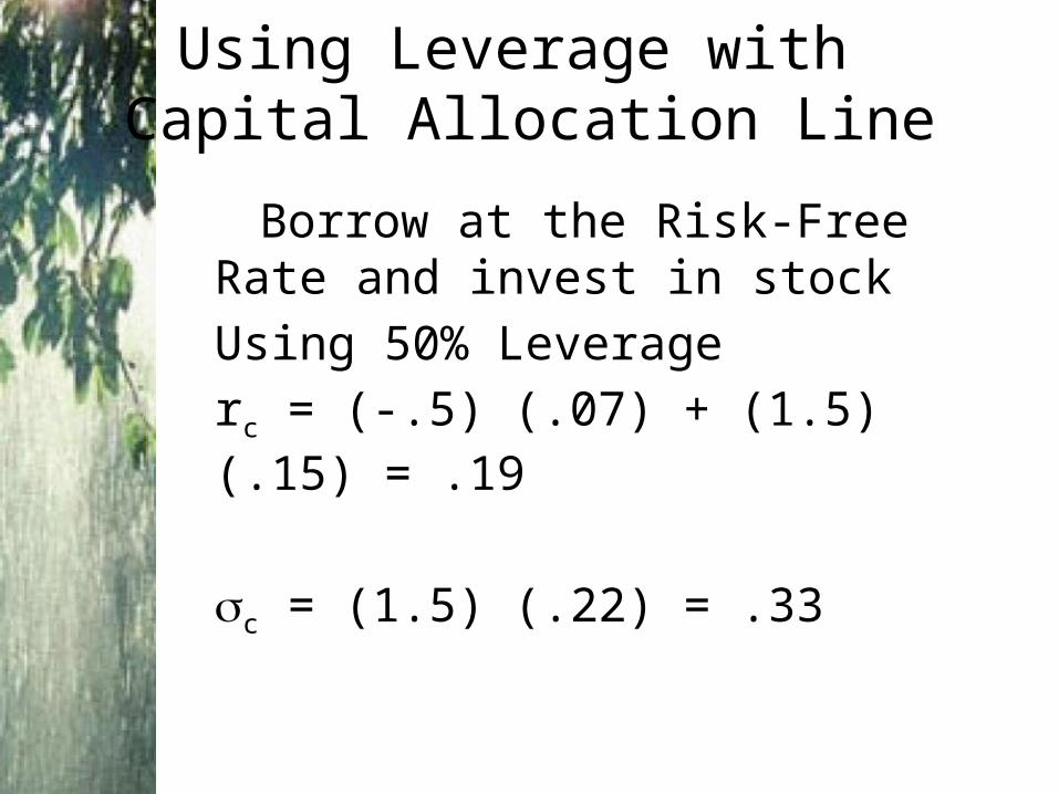
Using Leverage with Capital Allocation Line

Borrow at the Risk-Free Rate and invest in stock

Using 50% Leverage

rc = (-.5) (.07) + (1.5) (.15) = .19

sc = (1.5) (.22) = .33

Investment Opportunity Set with a Risk-Free Investment

Risk Aversion and Allocation

• Greater levels of risk aversion lead to larger proportions of the risk free rate

• Lower levels of risk aversion lead to larger proportions of the portfolio of risky assets

• Willingness to accept high levels of risk for high levels of returns would result in leveraged combinations

ASSET ALLOCATION WITH TWO RISKY ASSETS

Covariance and Correlation

• Portfolio risk depends on the correlation between the returns of the assets in the portfolio

• Covariance and the correlation coefficient provide a measure of the returns on two assets to vary either in tandem or in opposition

Two-Asset Portfolio Return: Stock and Bond

ReturnStock

htStock Weig

Return Bond

WeightBond

Return Portfolio

S

S

B

B

P

SSBBp

r

w

r

w

r

r rwrw

Covariance and Correlation Coefficient

• Covariance:

• Correlation Coefficient:

1

( , ) ( ) ( ) ( )S

S B S S B Bi

Cov r r p i r i r r i r

( , )S BSB

S B

Cov r r

Correlation Coefficients: Possible Values

If r = 1.0, the securities would be perfectly positively correlated

If r = - 1.0, the securities would be perfectly negatively correlated

Range of values for r 1,2

-1.0 < r < 1.0

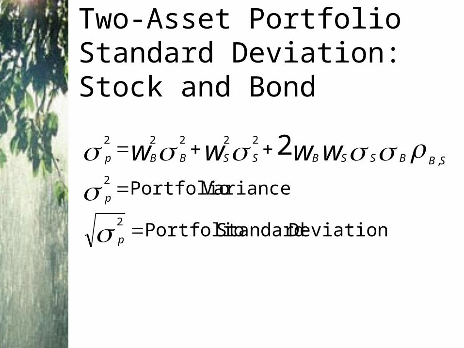
Two-Asset Portfolio Standard Deviation: Stock and Bond

Deviation Standard Portfolio

Variance Portfolio

2

2

,

22222 2

p

p

SBBSSBSSBBp wwww

Two-Risky-Asset Portfolio

• Rate of return on the portfolio:

• Expected rate of return on the portfolio:

P B B S Sr w r w r

( ) ( ) ( )P B B S SE r w E r w E r

Two-Risky-Asset Portfolio

• Variance of the rate of return on the portfolio:

2 2 2( ) ( ) 2( )( )P B B S S B B S S BSw w w w

Numerical Example: Bond and Stock Returns

ReturnsBond = 6% Stock = 10%

Standard Deviation Bond = 12% Stock = 25%

WeightsBond = .5 Stock = .5

Correlation Coefficient (Bonds and Stock) = 0

Numerical Example: Bond and Stock Returns

Return = 8%

.5(6) + .5 (10)

Standard Deviation = 13.87%

[(.5)2 (12)2 + (.5)2 (25)2 + …

2 (.5) (.5) (12) (25) (0)] ½

[192.25] ½ = 13.87

Investment Opportunity Set for Stocks and Bonds

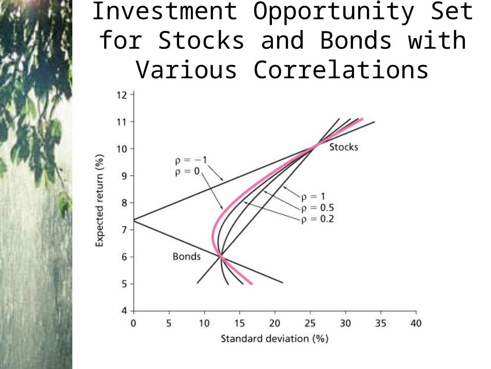
Investment Opportunity Set for Stocks and Bonds with Various Correlations

THE OPTIMAL RISKY PORTFOLIO WITH A RISK-FREE ASSET

Extending to Include Riskless Asset

• The optimal combination becomes linear• A single combination of risky and

riskless assets will dominate

Opportunity Set Using Stocks and Bonds and Two Capital Allocation Lines

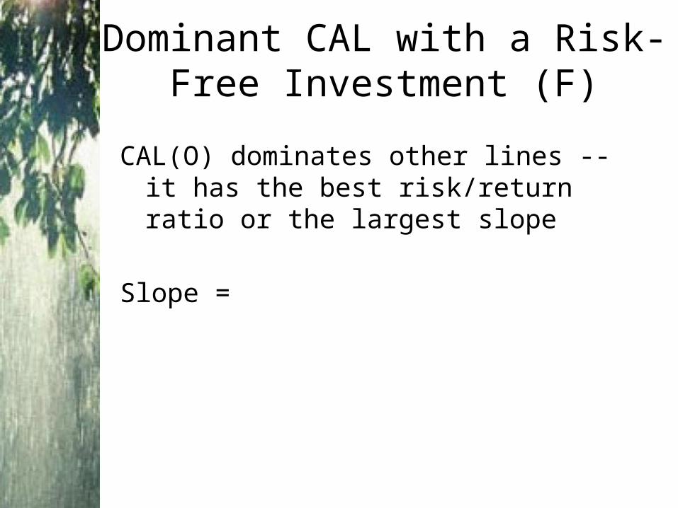
Dominant CAL with a Risk-Free Investment (F)

CAL(O) dominates other lines -- it has the best risk/return ratio or the largest slope

Slope = ( )A f

A

E r r

Optimal Capital Allocation Line for Bonds, Stocks and T-Bills

The Complete Portfolio

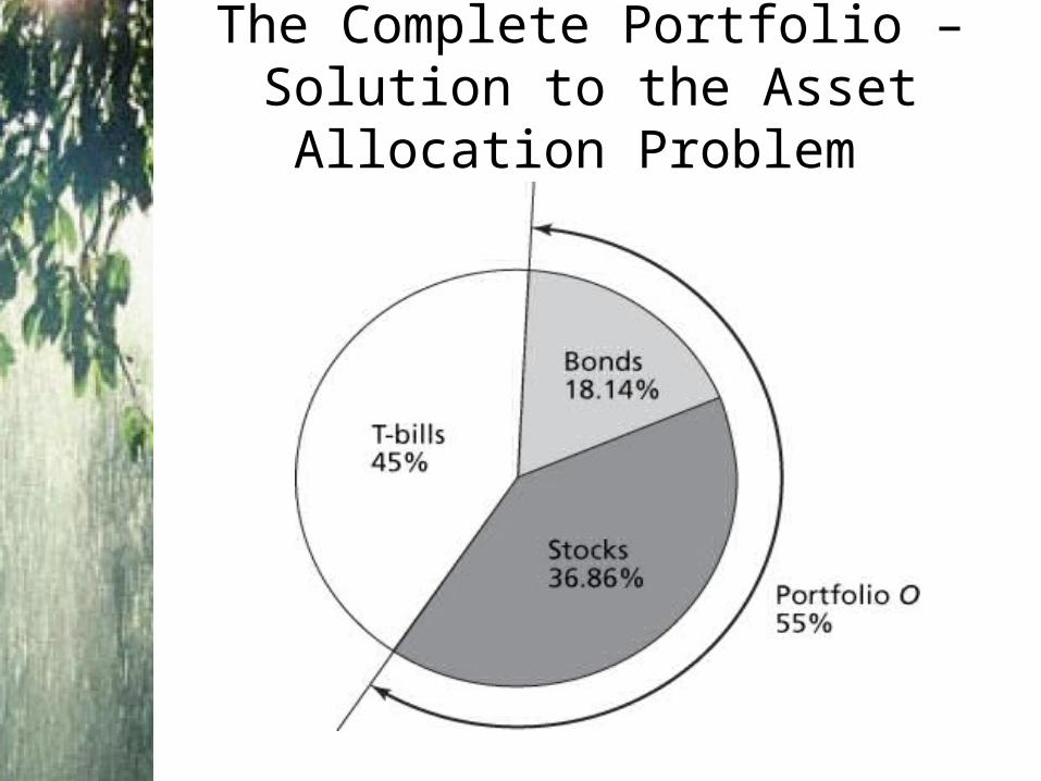
The Complete Portfolio – Solution to the Asset Allocation Problem

EFFICIENT DIVERSIFICATION WITH MANY RISKY ASSETS

Extending Concepts to All Securities

• The optimal combinations result in lowest level of risk for a given return

• Markowitz Portfolio Theory– a single asset or portfolio of assets is

considered to be efficient if no other asset or portfolio of assets offers higher expected return with the same (or lower) risk, or lower risk with the same (or higher) expected return.

Portfolios Constructed from Three Stocks A, B and C

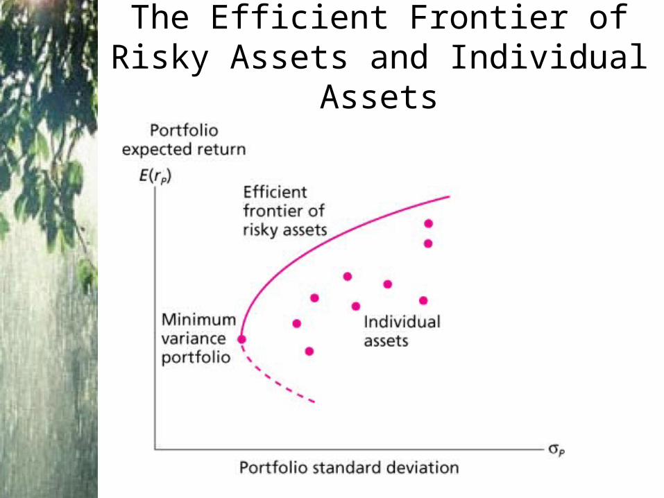
The Efficient Frontier of Risky Assets and Individual Assets