efficient incoherent ray traversal on gpus through...

Efficient Incoherent Ray Traversal on GPUs ThroughCompressed Wide BVHs

Henri Ylitie

NVIDIA

Tero Karras

NVIDIA

Samuli Laine

NVIDIA

8 kB

4 kB

0 kB

1 kB

2 kB

3 kB

5 kB

6 kB

7 kB

(a) (b) (c) (d)

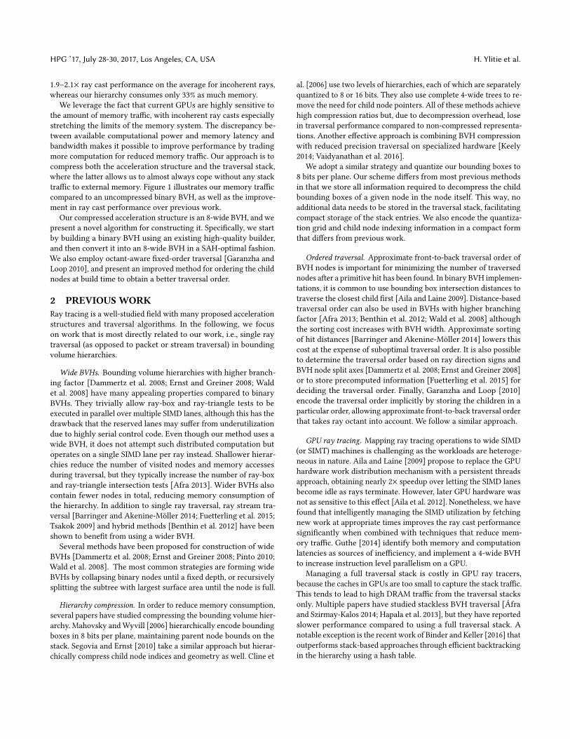
Figure 1: Our method reduces the memory traffic generated by ray casts, leading to significant performance improvement for

incoherent rays. (a) Two example scenes. (b) Node and triangle traffic generated by Aila et al. [2012]. (c) Traffic generated by

our method. (d) Ray cast performance as a function of bounce count for the top scene. Bounce 0 corresponds to primary rays.

ABSTRACT

We present a GPU-based ray traversal algorithm that operates

on compressed wide BVHs and maintains the traversal stack in a

compressed format. Our method reduces the amount of memory

traffic significantly, which translates to 1.9–2.1× improvement in

incoherent ray traversal performance compared to the current state

of the art. Furthermore, the memory consumption of our hierarchy

is 35–60% of a typical uncompressed BVH.

In addition, we present an algorithmically efficient method for

converting a binary BVH into a wide BVH in a SAH-optimal fashion,

and an improved method for ordering the child nodes at build time

for the purposes of octant-aware fixed-order traversal.

CCS CONCEPTS

• Computing methodologies→ Ray tracing; Graphics proces-

sors;

Permission to make digital or hard copies of all or part of this work for personal or

classroom use is granted without fee provided that copies are not made or distributed

for profit or commercial advantage and that copies bear this notice and the full citation

on the first page. Copyrights for components of this work owned by others than the

author(s) must be honored. Abstracting with credit is permitted. To copy otherwise, or

republish, to post on servers or to redistribute to lists, requires prior specific permission

and/or a fee. Request permissions from [email protected].

HPG ’17, Los Angeles, CA, USA© 2017 Copyright held by the owner/author(s). Publication rights licensed to ACM.

978-1-4503-5101-0/17/07. . . $15.00

DOI: 10.1145/3105762.3105773

KEYWORDS

Ray tracing, GPU, acceleration structures

ACM Reference format:

Henri Ylitie, Tero Karras, and Samuli Laine. 2017. Efficient Incoherent Ray

Traversal on GPUs Through Compressed Wide BVHs. In Proceedings of HPG’17, Los Angeles, CA, USA, July 28-30, 2017, 13 pages.DOI: 10.1145/3105762.3105773

1 INTRODUCTION

Ray casting continues to be an important primitive operation with

applications in realistic computer graphics, scientific visualization,

and simulation. The evolution of both CPU and GPU hardware has

sparked a lot of research investigating how to implement ray casting

most efficiently on modern hardware, and our paper continues

this tradition on the GPU side with a focus on recent NVIDIA

hardware. Our focus is primarily on incoherent rays, as they are

currently the most taxing workloads for GPU ray casting, and are

the predominant case in high-quality rendering.

Most often a tradeoff has to be made between performance and

memory usage, as more efficient algorithms tend to consume more

memory. Our method does not follow this rule of thumb—we simul-

taneously demonstrate a significant improvement in incoherent ray

cast performance, as well as reduced memory usage. Comparing to

the fastest previous method by Binder and Keller [2016], we achieve

HPG ’17, July 28-30, 2017, Los Angeles, CA, USA H. Ylitie et al.

1.9–2.1× ray cast performance on the average for incoherent rays,

whereas our hierarchy consumes only 33% as much memory.

We leverage the fact that current GPUs are highly sensitive to

the amount of memory traffic, with incoherent ray casts especially

stretching the limits of the memory system. The discrepancy be-

tween available computational power and memory latency and

bandwidth makes it possible to improve performance by trading

more computation for reduced memory traffic. Our approach is to

compress both the acceleration structure and the traversal stack,

where the latter allows us to almost always cope without any stack

traffic to external memory. Figure 1 illustrates our memory traffic

compared to an uncompressed binary BVH, as well as the improve-

ment in ray cast performance over previous work.

Our compressed acceleration structure is an 8-wide BVH, and we

present a novel algorithm for constructing it. Specifically, we start

by building a binary BVH using an existing high-quality builder,

and then convert it into an 8-wide BVH in a SAH-optimal fashion.

We also employ octant-aware fixed-order traversal [Garanzha and

Loop 2010], and present an improved method for ordering the child

nodes at build time to obtain a better traversal order.

2 PREVIOUS WORK

Ray tracing is a well-studied field with many proposed acceleration

structures and traversal algorithms. In the following, we focus

on work that is most directly related to our work, i.e., single ray

traversal (as opposed to packet or stream traversal) in bounding

volume hierarchies.

Wide BVHs. Bounding volume hierarchies with higher branch-

ing factor [Dammertz et al. 2008; Ernst and Greiner 2008; Wald

et al. 2008] have many appealing properties compared to binary

BVHs. They trivially allow ray-box and ray-triangle tests to be

executed in parallel over multiple SIMD lanes, although this has the

drawback that the reserved lanes may suffer from underutilization

due to highly serial control code. Even though our method uses a

wide BVH, it does not attempt such distributed computation but

operates on a single SIMD lane per ray instead. Shallower hierar-

chies reduce the number of visited nodes and memory accesses

during traversal, but they typically increase the number of ray-box

and ray-triangle intersection tests [Afra 2013]. Wider BVHs also

contain fewer nodes in total, reducing memory consumption of

the hierarchy. In addition to single ray traversal, ray stream tra-

versal [Barringer and Akenine-Möller 2014; Fuetterling et al. 2015;

Tsakok 2009] and hybrid methods [Benthin et al. 2012] have been

shown to benefit from using a wider BVH.

Several methods have been proposed for construction of wide

BVHs [Dammertz et al. 2008; Ernst and Greiner 2008; Pinto 2010;

Wald et al. 2008]. The most common strategies are forming wide

BVHs by collapsing binary nodes until a fixed depth, or recursively

splitting the subtree with largest surface area until the node is full.

Hierarchy compression. In order to reduce memory consumption,

several papers have studied compressing the bounding volume hier-

archy. Mahovsky andWyvill [2006] hierarchically encode bounding

boxes in 8 bits per plane, maintaining parent node bounds on the

stack. Segovia and Ernst [2010] take a similar approach but hierar-

chically compress child node indices and geometry as well. Cline et

al. [2006] use two levels of hierarchies, each of which are separately

quantized to 8 or 16 bits. They also use complete 4-wide trees to re-

move the need for child node pointers. All of these methods achieve

high compression ratios but, due to decompression overhead, lose

in traversal performance compared to non-compressed representa-

tions. Another effective approach is combining BVH compression

with reduced precision traversal on specialized hardware [Keely

2014; Vaidyanathan et al. 2016].

We adopt a similar strategy and quantize our bounding boxes to

8 bits per plane. Our scheme differs from most previous methods

in that we store all information required to decompress the child

bounding boxes of a given node in the node itself. This way, no

additional data needs to be stored in the traversal stack, facilitating

compact storage of the stack entries. We also encode the quantiza-

tion grid and child node indexing information in a compact form

that differs from previous work.

Ordered traversal. Approximate front-to-back traversal order of

BVH nodes is important for minimizing the number of traversed

nodes after a primitive hit has been found. In binary BVH implemen-

tations, it is common to use bounding box intersection distances to

traverse the closest child first [Aila and Laine 2009]. Distance-based

traversal order can also be used in BVHs with higher branching

factor [Afra 2013; Benthin et al. 2012; Wald et al. 2008] although

the sorting cost increases with BVH width. Approximate sorting

of hit distances [Barringer and Akenine-Möller 2014] lowers this

cost at the expense of suboptimal traversal order. It is also possible

to determine the traversal order based on ray direction signs and

BVH node split axes [Dammertz et al. 2008; Ernst and Greiner 2008]

or to store precomputed information [Fuetterling et al. 2015] for

deciding the traversal order. Finally, Garanzha and Loop [2010]

encode the traversal order implicitly by storing the children in a

particular order, allowing approximate front-to-back traversal order

that takes ray octant into account. We follow a similar approach.

GPU ray tracing. Mapping ray tracing operations to wide SIMD

(or SIMT) machines is challenging as the workloads are heteroge-

neous in nature. Aila and Laine [2009] propose to replace the GPU

hardware work distribution mechanism with a persistent threads

approach, obtaining nearly 2× speedup over letting the SIMD lanes

become idle as rays terminate. However, later GPU hardware was

not as sensitive to this effect [Aila et al. 2012]. Nonetheless, we have

found that intelligently managing the SIMD utilization by fetching

new work at appropriate times improves the ray cast performance

significantly when combined with techniques that reduce mem-

ory traffic. Guthe [2014] identify both memory and computation

latencies as sources of inefficiency, and implement a 4-wide BVH

to increase instruction level parallelism on a GPU.

Managing a full traversal stack is costly in GPU ray tracers,

because the caches in GPUs are too small to capture the stack traffic.

This tends to lead to high DRAM traffic from the traversal stacks

only. Multiple papers have studied stackless BVH traversal [Áfra

and Szirmay-Kalos 2014; Hapala et al. 2013], but they have reported

slower performance compared to using a full traversal stack. A

notable exception is the recent work of Binder and Keller [2016] that

outperforms stack-based approaches through efficient backtracking

in the hierarchy using a hash table.

Efficient Incoherent Ray Traversal on GPUs Through Compressed Wide BVHs HPG ’17, July 28-30, 2017, Los Angeles, CA, USA

Ray-node tests Ray-triangle tests

Bounce 0 1 4 0 1 4

Full precision 14.30 14.54 14.62 6.45 7.64 8.61

8 bits 14.69 14.95 15.02 6.59 7.98 9.03

7 bits 15.04 15.32 15.38 6.73 8.23 9.31

6 bits 15.69 16.03 16.06 7.01 8.70 9.81

5 bits 17.18 17.53 17.50 7.62 9.56 10.76

4 bits 20.56 20.86 20.67 8.94 11.36 12.71

Table 1: Effect of AABB quantization on intersection test

counts. The numbers represent arithmetic means over our

test scenes, excluding Powerplant.

Ray-node tests Ray-triangle tests

Bounce 0 1 4 0 1 4

Distance order 13.43 14.03 13.99 5.32 6.99 7.91

Octant order 14.69 14.95 15.02 6.59 7.98 9.03

Random order 17.65 17.45 18.62 10.28 11.04 13.60

Table 2: Effect of traversal order on intersection test counts.

The numbers represent arithmetic means over our test

scenes, excluding Powerplant.

3 COMPRESSEDWIDE BVH

Our acceleration structure is a compressed 8-wide BVH that uses

axis-aligned bounding boxes (AABBs) as the bounding volumes.

The high branching factor amortizes the memory fetch latencies

over 8 bounding box intersection tests and increases instruction

level parallelism during internal node tests.

We compress both bounding boxes and child pointers so that our

internal nodes require only ten bytes per child, obtaining 1 : 3.2

compression ratio compared to the standard uncompressed BVH

node format. This provides an immediate reduction in the amount of

memory traffic. Secondarily, thanks to the small memory footprint,

more nodes fit in the GPU caches, which further reduces the most

expensive external memory traffic.

3.1 Child Bounding Box Compression

Similarly to previous methods [Keely 2014; Mahovsky and Wyvill

2006; Segovia and Ernst 2010; Vaidyanathan et al. 2016], we quantize

child node AABBs to a local grid and store locations of the AABB

planes with a small number of bits.1Specifically, given the common

bounding box Blo ,Bhi that covers all children, we store the originpoint of the local grid p = Blo as three floating-point values. The

coordinates of the child AABBs are stored as unsigned integers

using Nq = 8 bits per plane. The scale of the grid on each axis

i ∈ {x ,y, z} is constrained to be a power of two 2ei, where ei

is chosen to be the smallest integer that allows representing the

maximum plane of the common AABB in Nq bits without overflow,

i.e., Bhi,i ≤ pi + 2ei (2Nq − 1). From this constraint we obtain

ei =

⌈log

2

Bhi,i − pi

2Nq − 1

⌉. (1)

In practice, we represent the scale 2ei

as a 32-bit floating-point

number but store only the 8 exponent bits, as the remaining bits

1For an illustration, we refer the reader to Figure 1 by Vaidyanathan et al. [2016].

00 01

1110

x

yray

order[0]

order[1]

order[2]

order[3]

oct 00

00

00

00

00

01

01

01

01

01

10

10

10

10

10

11

11

11

11

11

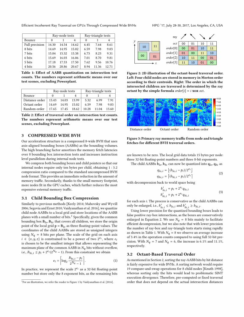
Figure 2: 2D illustration of the octant-based traversal order.

Left: Four child nodes are stored inmemory inMorton order

according to their centroids. Right: The order in which the

intersected children are traversed is determined by the ray

octant by the simple formula order[i] = i xor oct.

8 kB

4 kB

0 kB

1 kB

2 kB

3 kB

5 kB

6 kB

7 kB

Distance order Octant order Random order

Figure 3: Primary raymemory traffic fromnode and triangle

fetches for different BVH traversal orders.

are known to be zero. The local grid data totals 15 bytes per node:

three 32-bit floating-point numbers and three 8-bit exponents.

The child AABBs blo , bhi can now be quantized into qlo , qhi as

qlo,i =⌊(blo,i − pi )/2

ei⌋

qhi,i =⌈(bhi,i − pi )/2

ei⌉ (2)

with decompression back to world space being

b ′lo,i = pi + 2eiqlo,i

b ′hi,i = pi + 2eiqhi,i

(3)

for each axis i . The process is conservative as the child AABBs can

only be enlarged, i.e., b ′lo,i ≤ blo,i and b′hi,i ≥ bhi,i .

Using lower precision for the quantized bounding boxes leads to

false positive ray-box intersections, as the boxes are conservatively

enlarged in Equation 2. We use Nq = 8 bits mainly to facilitate

efficient decompression, but we also note that with lower precision

the number of ray-box and ray-triangle tests starts rising rapidly

as shown in Table 1. With Nq = 8 we observe an average increase

of 3.4% in the operation counts compared to using full 32-bit pre-

cision. With Nq = 7 and Nq = 6, the increase is 6.1% and 11.1%,

respectively.

3.2 Octant-Based Traversal Order

Asmentioned in Section 2, sorting the ray-AABB hits by hit distance

is fairly expensive for wide BVHs. A sorting network would require

19 compare-and-swap operations for 8 child nodes [Knuth 1998],

whereas sorting only the hits would lead to problematic SIMT

execution divergence. Therefore, pre-computed or fixed traversal

order that does not depend on the actual intersection distances


Child

0

child node base index triangle base index

Child

1

Child

2

Child

3

Child

4

Child

5

Child

6

Child

7

px pypz ex ey ez imask

metaqlo,xqlo,yqlo,zqhi,xqhi,yqhi,z

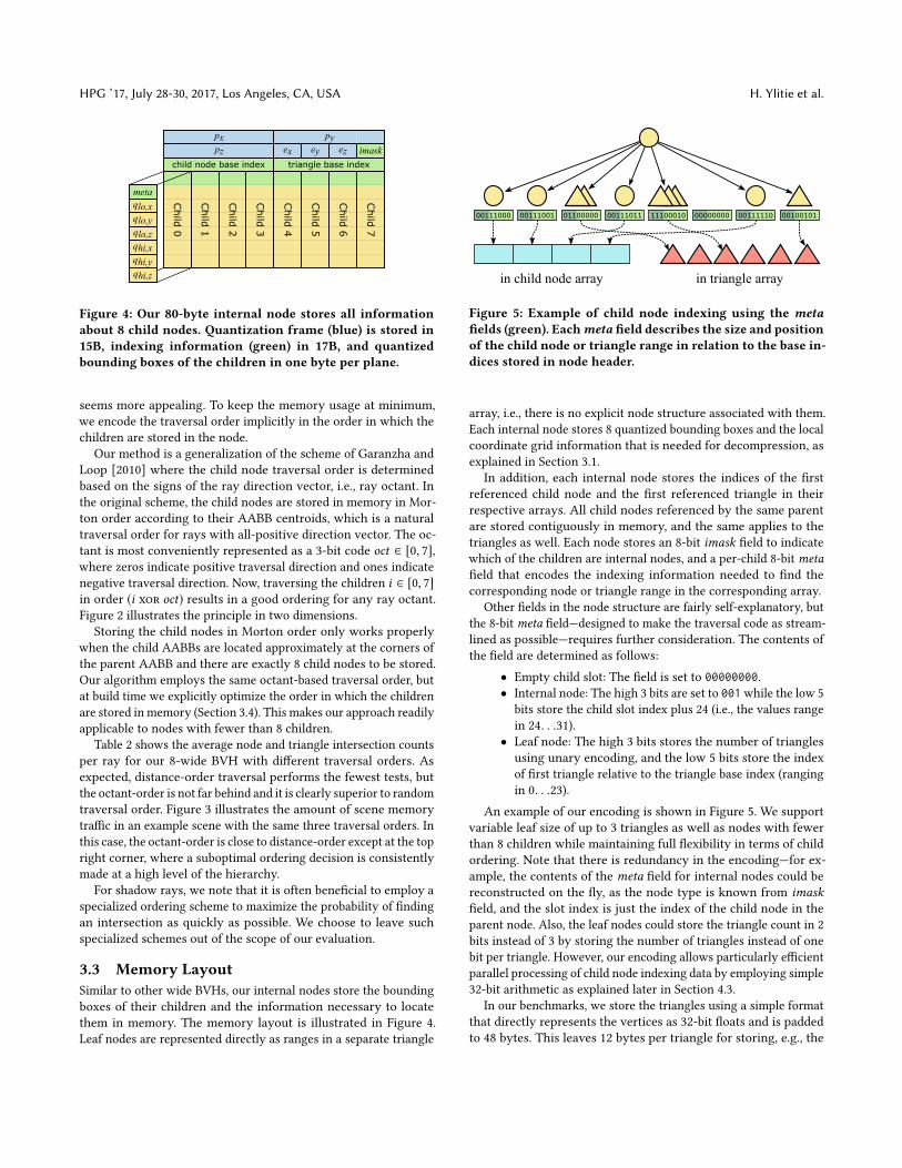
Figure 4: Our 80-byte internal node stores all information

about 8 child nodes. Quantization frame (blue) is stored in

15B, indexing information (green) in 17B, and quantized

bounding boxes of the children in one byte per plane.

seems more appealing. To keep the memory usage at minimum,

we encode the traversal order implicitly in the order in which the

children are stored in the node.

Our method is a generalization of the scheme of Garanzha and

Loop [2010] where the child node traversal order is determined

based on the signs of the ray direction vector, i.e., ray octant. In

the original scheme, the child nodes are stored in memory in Mor-

ton order according to their AABB centroids, which is a natural

traversal order for rays with all-positive direction vector. The oc-

tant is most conveniently represented as a 3-bit code oct ∈ [0, 7],where zeros indicate positive traversal direction and ones indicate

negative traversal direction. Now, traversing the children i ∈ [0, 7]in order (i xor oct) results in a good ordering for any ray octant.

Figure 2 illustrates the principle in two dimensions.

Storing the child nodes in Morton order only works properly

when the child AABBs are located approximately at the corners of

the parent AABB and there are exactly 8 child nodes to be stored.

Our algorithm employs the same octant-based traversal order, but

at build time we explicitly optimize the order in which the children

are stored in memory (Section 3.4). This makes our approach readily

applicable to nodes with fewer than 8 children.

Table 2 shows the average node and triangle intersection counts

per ray for our 8-wide BVH with different traversal orders. As

expected, distance-order traversal performs the fewest tests, but

the octant-order is not far behind and it is clearly superior to random

traversal order. Figure 3 illustrates the amount of scene memory

traffic in an example scene with the same three traversal orders. In

this case, the octant-order is close to distance-order except at the top

right corner, where a suboptimal ordering decision is consistently

made at a high level of the hierarchy.

For shadow rays, we note that it is often beneficial to employ a

specialized ordering scheme to maximize the probability of finding

an intersection as quickly as possible. We choose to leave such

specialized schemes out of the scope of our evaluation.

3.3 Memory Layout

Similar to other wide BVHs, our internal nodes store the bounding

boxes of their children and the information necessary to locate

them in memory. The memory layout is illustrated in Figure 4.

Leaf nodes are represented directly as ranges in a separate triangle

in child node array in triangle array

00111001 01100000 00111011 11100010 00000000 00111110 0010010100111000

Figure 5: Example of child node indexing using the metafields (green). Eachmeta field describes the size and position

of the child node or triangle range in relation to the base in-

dices stored in node header.

array, i.e., there is no explicit node structure associated with them.

Each internal node stores 8 quantized bounding boxes and the local

coordinate grid information that is needed for decompression, as

explained in Section 3.1.

In addition, each internal node stores the indices of the first

referenced child node and the first referenced triangle in their

respective arrays. All child nodes referenced by the same parent

are stored contiguously in memory, and the same applies to the

triangles as well. Each node stores an 8-bit imask field to indicate

which of the children are internal nodes, and a per-child 8-bit metafield that encodes the indexing information needed to find the

corresponding node or triangle range in the corresponding array.

Other fields in the node structure are fairly self-explanatory, but

the 8-bit meta field—designed to make the traversal code as stream-

lined as possible—requires further consideration. The contents of

the field are determined as follows:

• Empty child slot: The field is set to 00000000.• Internal node: The high 3 bits are set to 001while the low 5

bits store the child slot index plus 24 (i.e., the values range

in 24. . .31).

• Leaf node: The high 3 bits stores the number of triangles

using unary encoding, and the low 5 bits store the index

of first triangle relative to the triangle base index (ranging

in 0. . .23).

An example of our encoding is shown in Figure 5. We support

variable leaf size of up to 3 triangles as well as nodes with fewer

than 8 children while maintaining full flexibility in terms of child

ordering. Note that there is redundancy in the encoding—for ex-

ample, the contents of the meta field for internal nodes could be

reconstructed on the fly, as the node type is known from imaskfield, and the slot index is just the index of the child node in the

parent node. Also, the leaf nodes could store the triangle count in 2

bits instead of 3 by storing the number of triangles instead of one

bit per triangle. However, our encoding allows particularly efficient

parallel processing of child node indexing data by employing simple

32-bit arithmetic as explained later in Section 4.3.

In our benchmarks, we store the triangles using a simple format

that directly represents the vertices as 32-bit floats and is padded

to 48 bytes. This leaves 12 bytes per triangle for storing, e.g., the


original triangle index in the input mesh. We sort the clusters of

contiguous nodes and triangles in depth-first order for maximum

performance, but our method does not depend on such global or-

dering for correctness. Using random order instead of depth-first

order has no effect on performance of primary rays, but it slows

down diffuse bounces 1–8 by 0%–10% depending on the scene.

3.4 Optimal Wide BVH Construction

Our goal is to establish a firm baseline in terms of the maximum ray

tracing performance that can be achieved using compressed wide

BVHs. For the highest possible BVH quality, we employ a CPU-

based offline algorithm that first constructs a high-quality binary

BVH and then collapses its nodes into wide nodes in a SAH-optimal

fashion. The topology of the resulting wide BVH is constrained by

the topology of the initial binary BVH, and we only minimize the

SAH cost under this constraint.

The initial binary BVH is built using the SBVH algorithm of Stich

et al. [2009] with one primitive per leaf. This yields a high-quality

binary BVH with controllable amount of spatial triangle splitting.

To convert the binary BVH into a wide BVH, we use a dynamic

programming approach similar to the method used by Aila and

Karras [2010] for splitting a BVH into clusters that fit in local caches,

as well as to the method used by Pinto [2010] for collapsing nodes

to reduce ray-box tests. Our main difference to these methods is

that we jointly optimize both internal nodes and leaf nodes at the

same time, reaching a global optimum with respect to them both.

The goal of the construction is tominimize the total SAH cost [Gold-

smith and Salmon 1987;MacDonald and Booth 1990] of the resulting

wide BVH:

SAH =∑n∈I

An · cnode +∑n∈L

An · Pn · cprim , (4)

where I and L correspond to the set of internal nodes and the

set of leaf nodes, respectively, An is the AABB surface area of

node n expressed relative to the surface area of the root, Pn is

the number of primitives in leaf node n, and cnode and cprim are

constants that represent the cost of ray-node test and ray-triangle

test, respectively.

We minimize Equation 4 by computing and storing, for each

node n in the binary BVH, the optimal SAH cost C(n, i) that can be

achieved if the contents of the entire subtree of n were represented

as a forest of at most i BVHs. We only consider i ∈ [1, 7] for thepurposes of our 8-wide BVH construction. After computation, the

optimal SAH cost of the entire hierarchy represented as a single

wide BVH is thus available at C(root, 1). The actual constructionof the wide BVH is performed after the cost computation pass is

finished.

The cost computation is done in a bottom-up fashion in the

binary hierarchy, i.e., a node is processed only after both of its

children have been processed. This ensures that all the data required

to compute C(n, i) is already available by the time we visit node

n. At the leaves of the binary BVH, each containing one primitive,

we simply set C(n, i) = An · cprim for all i ∈ [1, 7]. At the internalnodes, we calculate cost C(n, i) as follows:

C(n, i) =

{min

(Cleaf (n), Cinternal(n)

)if i = 1

min

(Cdistribute(n, i), C(n, i − 1)

)otherwise

(5)

The first case corresponds to creating a new wide BVH node to

serve as the root of the subtree at n, and we can either choose to

create a leaf node or an internal node. The second case corresponds

to creating a forest with up to i roots, and we need to find the

optimal way to distribute these roots into left and right subtree of

n. Alternatively, we may decide to create fewer than i roots.Creating a leaf node is only possible when there are few enough

primitives in the subtree of n:

Cleaf (n) =

{An · Pn · cprim if Pn ≤ Pmax

∞ otherwise

(6)

Here Pn represents the total number of primitives under node nand Pmax is the maximum allowed leaf size for the wide BVH.

Creating an internal node at n requires us to select up to 8 de-

scendant nodes to serve as its children. The minimum SAH cost

of these nodes is given by Cdistribute(n, 8), and we only need to add

the cost term associated with n itself:

Cinternal(n) = Cdistribute(n, 8) +An · cnode (7)

Finally, we define function Cdistribute(n, j) to give the optimal cost

of representing the entire subtree of n using a forest of at least two

and at most j BVHs:

Cdistribute(n, j) = min

0<k<j

(C(nleft ,k) +C(nright , j − k)

)(8)

where nleft and nright are the left and right child nodes of n. Theminimum is taken over the different ways of distributing at most kof the roots in the left subtree of n, and at most j − k roots in the

right subtree.

During the cost computation we also store the decisions that

yielded the optimal C(n, i) for each n and i . After the cost com-

putation is complete, we backtrack these decisions starting from

C(root, 1) and create wide BVH nodes so that the optimal cost is

realized. This finishes the topology construction of the wide BVH.

Child node ordering. As explained in Section 3.2, there is no tra-

versal order related data stored in the nodes, and the traversal order

is implicitly encoded into the order of the child nodes. Based on

our octant-based traversal order, we have a conceptually simple

optimization problem: Our goal is to ensure that, for all ray direc-

tions, the child nodes will be traversed in an order that matches

the distance-order as closely as possible.

In principle, we could enumerate every possible ordering for the

child nodes and pick the one that closest approximates the distance-

order for differently oriented rays. Unfortunately, due to the high

number of possible orderings (8! = 40320) this is hardly feasible in

practice.

We experimented with various methods and cost functions for

determining the child node ordering, and found that many approxi-

mate methods produced essentially identical results that could not

be improved further. We thus settled for the simplest algorithm we

found that was in this class. For each node, we start by filling a 8×8

table cost(c, s), where each table cell indicates the cost of placing

a particular child node c in a particular child slot s ∈ [0, 7]. Fromthis data, the assignment that minimizes the total cost can be found

efficiently using the auction algorithm [Bertsekas 1992].

To define cost(c, s), we consider a diagonal ray with direction

ds = (±1,±1,±1) that would traverse slot s first according to the


octant-order. The sign of the ith component of ds is based on the

ith bit of s , so that zero corresponds to + and one corresponds to −.

We compute the cost for each of the eight sign combinations as the

difference between the parent node centroid p and the child node

centroid c, projected on the corresponding diagonal ray direction:

cost(c, s) = (c − p) · ds . (9)

Build time. Our current implementation takes about 6 minutes

to construct the wide BVH for a scene consisting of 10M triangles.

Roughly 80% of the time goes to initial binary BVH construction,

14% to node collapsing, and 6% to child node ordering. We believe

that the build time could be improved considerably through simple

optimizations.

4 TRAVERSAL ALGORITHM

Our BVH traversal algorithm is loosely based on the binary BVH

traversal of Aila and Laine [2009]. We adopt the use of persistent

threads and dynamic ray fetching based on SIMD utilization heuris-

tics andmap each ray to a single CUDA thread. Themain differences

are in traversal stack management, traversal order determination,

and internal node decompression. We use a compressed traversal

stack in which each entry may contain several children of an 8-

wide BVH node. Memory traffic caused by the traversal stack has

traditionally consumed a large part of available memory bandwidth

on GPUs [Aila and Karras 2010], but we remove practically all of it

through compression and the use of shared memory.

Algorithm 1 BVH traversal

1: r ← FetchRay() // Origin, direction, tmin, and tmax2: S ← ∅ // Traversal stack

3: G ← {root} // Current node group

4: loop

5: if G represents a node group then

6: n ← GetClosestNode(G, r )7: G ← G \ n8: if G , ∅ then StackPush(G, S)9: G,Gt ← IntersectChildren(n, r )10: else // G represents a triangle group

11: Gt ← G12: G ← ∅13: end if

14: while Gt , ∅15: if ratio of active threads is too low then

16: StackPush(Gt , S)17: break

18: end if

19: t ← GetNextTriangle(Gt )

20: Gt ← Gt \ t21: IntersectTriangle(t , r )22: end while

23: if G = ∅ then24: if S = ∅ then break // Traversal finished

25: G ← StackPop(S)

26: end if

27: end loop

triangle base index

child node base index hits

32 8

32

imask

8

pad

16

pad

8

triangle hits

24

Figure 6: Traversal stack entries for a group of internal

nodes (top) and a group of triangles (bottom). Both are

padded to 64 bits and can reference up to 8 nodes or 24 tri-

angles.

Algorithm 1 presents a simplified pseudocode for traversing a

single ray using a single CUDA thread. For the sake of clarity, the

pseudocode does not reflect the use of persistent threads or dynamic

ray fetching. We defer discussion of these features to Section 4.4.

The traversal stack S is initially empty, as we maintain its top

entry G, or current node group, in registers. Each stack entry may

refer to one or more internal nodes referenced by the same parent,

or one or more triangles referenced by one internal node. We never

mix internal nodes and triangles in the same group.

The main traversal loop begins on line 4. At the beginning of

each iteration, the current node group G is checked for which kind

of nodes it contains—by design, it is never empty between main

loop iterations. IfG contains internal nodes, we extract node n that

we should visit next according to the octant traversal order. If this

does not makeG empty, we push its remains to the stack. On line 9

we intersect the bounding boxes of all children in node n, whichmay yield both internal and leaf node hits. These form two separate

groups G and Gt for internal nodes and triangles, respectively.

Alternatively, ifG consisted of triangles instead of internal nodes

on line 5, its contents are moved to Gt on line 11 and G is cleared.

Next, we intersect the triangles in current triangle groupGt . We

keep intersecting triangles inGt until it becomes empty, or until the

ratio of threads performing triangle intersection test in the warp (i.e.

a group of 32 threads) falls below a threshold (Section 4.4). In the

latter case, we postpone the intersection of remaining triangles by

pushing Gt to the stack on line 16. The postponed triangle groups

are eventually tested in subsequent loop iterations when other

threads in the warp have hit leaf nodes or terminated.

Before continuing to the next iteration of the traversal loop, we

pop a new node group G from the stack if necessary. If both G and

the stack are empty, the traversal is finished.

4.1 Compressed Traversal Stack

The current node group G and triangle group Gt are stored in a

compressed format, and the same format is used when groups are

pushed into the stack. The current node group G is stored as a

64-bit node group entry as illustrated in Figure 6 (top). Similarly,

the current triangle group Gt is stored as a 64-bit triangle groupentry as illustrated in Figure 6 (bottom). These entries store the base

index to internal nodes or triangles, as well as a bit mask indicating

which nodes or triangles are active, i.e., whose bounding boxes were

intersected and which have not yet been processed. In addition,

the imask field from the internal node is stored for the node group

entries. To distinguish between the two types when executing a

stack pop, we look at bits 24–31, i.e., the byte occupied by the hits


field for node entries. If this byte is zero, we know that the entry is

a triangle group entry. Otherwise, it is a node group entry.

As an important implementation detail, we reorder the bits in

the hits field of the node group entry according to their priority

(slot_index ^ (7 - oct)) with respect to the octant-based tra-

versal order.2In other words, the children that should be traversed

first are represented by the highest bits while the children that

should be traversed last are represented by the lowest bits. This lets

us efficiently determine the next active child to traverse by finding

the highest set bit in this field.

To reduce external memory traffic during traversal, we store

the first N stack entries in SM-local shared memory. Because the

amount of shared memory is limited, it cannot accommodate the en-

tire stack in all situations, and thus we spill to thread-local memory

when the shared memory stack capacity is exceeded. In our imple-

mentation, at most 12 stack entries (96 bytes) can be stored in shared

memory per thread without reducing the number of simultaneously

active threads. As each level in the hierarchy produces 0–2 stack

entries, 12 entries are almost always sufficient and spilling happens

very rarely. In Section A.3 (Appendix) we present experimental

results for different shared memory stack sizes.

4.2 Node Decompression and Intersection

Careful implementation of the node intersection test and stack

management is crucial for traversal performance. We load both

internal nodes and triangles through the cache hierarchy using

128-bit wide vector load instructions.

Instead of transforming the quantized bounding boxes to world

space, we convert the 8-bit plane positions directly to floating-point

values, and transform the ray origin o and direction d to account

for the quantization grid origin and scale. This method is efficient

on NVIDIA hardware, because any byte in a 32-bit word can be

converted into a floating-point value with a single instruction. For

each axis i ∈ {x ,y, z}, the ray is adjusted as follows:

d ′i = 2ei /di

o′i = (pi − oi )/di(10)

The quantization grid scale 2ei

is formed by shifting the 8-bit ex-

ponent to the floating-point exponent bits while keeping the sign

and mantissa bits cleared. After this, we can compute the ray-plane

intersection distances with a single FMA instruction per plane:

tlo,i = qlo,id′i + o

′i

thi,i = qhi,id′i + o

′i

(11)

Similar to Aila et al. [2012], we employ VMIN, VMAX instructions

for efficient 3-way minimum and maximum in the intersection test.

We also use PRMT instruction to select the near and far planes of 4

quantized boxes at once before the test, depending on ray octant.

4.3 Traversal State Management

In addition to box decompression and intersection, the Inter-

sectChildren function on line 9 of Algorithm 1 is also responsible

for traversal order computations and forming the traversal stack

entries. We perform the traversal order computations described in

Section 4.1 in packed form for 4 children at once.

2Note that we explicitly reverse the order of the bits by using 7 − oct instead of oct.

To construct the hits field of the node group entry in accordance

to the octant traversal order, we need to compute the traversal pri-

ority (slot_index ^ (7 - oct)) for each child that corresponds

to an internal node. Using C syntax, the computation is done for 4

children in parallel as follows:

octinv4 = (7 - oct) * 0x01010101;is_inner4 = (meta4 & (meta4 << 1)) & 0x10101010;inner_mask4 = sign_extend_s8x4(is_inner4 << 3);bit_index4 = (meta4 ^ (octinv4 & inner_mask4)) & 0x1F1F1F1F;

Here each variable with a postfix 4 contains data for 4 different

child nodes. The calculation of is_inner4 exploits the fact that bits3 and 4 are set simultaneously only for internal nodes due to the

biasing of meta by 24. Function sign_extend_s8x4, implemented

using the PRMT instruction, sign extends each byte in a 32-bit word

individually with a single assembly instruction, producing a byte

mask for the internal nodes. In the end, each byte of bit_index4contains the traversal priority, biased by 24, for internal nodes, and

the triangle offset for leaf nodes.

Conveniently, the bytes in bit_index4 now indicate directly

where bits should be set in the hits and triangle hits fields in node

and triangle group entries for G and Gt . Remembering that the

highest 3 meta bits are 001 for internal nodes and contain one bit

per triangle for leaf nodes, we can construct the hits and trianglehits fields in G and Gt simultaneously, without considering which

type the child node is, by shifting the top 3meta bits to the positionindicated by the corresponding byte in bit_index4. Furthermore,

a non-existent child node has 000 as the high 3 bits of meta, so this

operation will not insert bits in either field.3Using C syntax again,

we first move the high 3 bits in meta fields to start from lowest bit

position, child_bits4 = (meta4 >> 5) & 0x07070707 and theninsert a given child in the hits and triangle hits fields as follows:

if (intersected) {child_bits = extract_byte(child_bits4, slot_index % 4);bit_index = extract_byte(bit_index4, slot_index % 4);hitmask = hitmask | (child_bits << bit_index);

}

We use loop unrolling to replicate the same operation for each of

the 8 child slots. The entire body of the if statementmaps to a single

PTX instruction vshl.u32.u32.u32.wrap.add r0,r1.b,r2.b,r3which in turn compiles to a single assembly instruction.

Obtaining the closest internal node inG on line 6 of Algorithm 1

works as follows: We find the index of the highest set bit in the hitsfield of the node group entry, and clear the bit to remove the node.

The corresponding child slot index is found by subtracting the bias

of 24 and reversing the traversal priority computation: slot_index= (bit_index - 24) ^ (7 - oct). Relative index of the node

is then obtained by computing the number of neighboring nodes

stored in the lower child slots: relative_index = popc(imask &

~(-1 << slot_index)). Selecting an active triangle from Gt on

line 19 is simpler, as the index of each set bit in triangle hits directlyindicates the relative index of the triangle.

3Even if we set the bounding box for a non-existing child as a maximally inverted

box, it may still be possible to intersect it due to roundoff errors. The zero meta fieldensures logical consistency even in this situation.


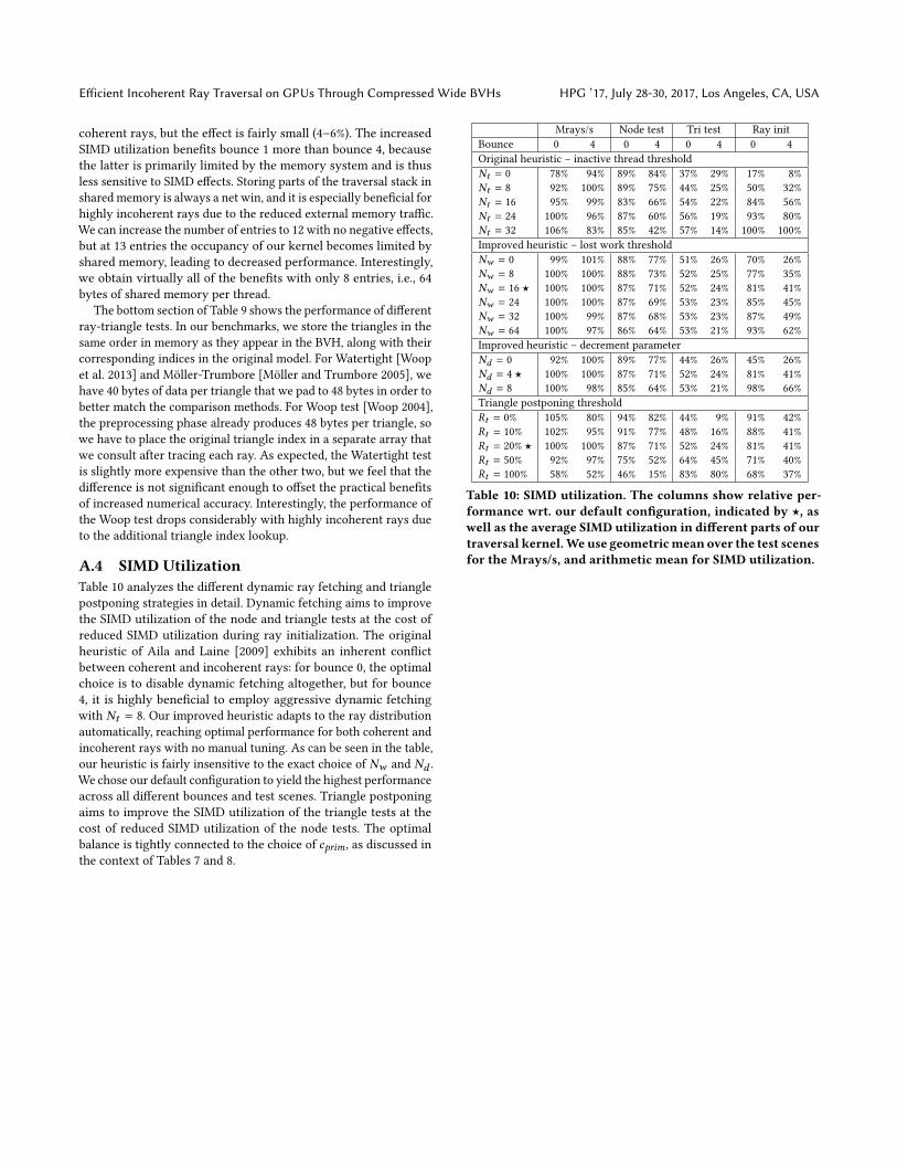
4.4 Improving SIMD Utilization

Ray tracingworkloads can be highly heterogeneous, causing threads

in a warp to finish traversal at different times. To avoid wasting

computational resources, we adopt persistent threads with dynamic

ray fetching from Aila and Laine [2009]. In their original heuristic,

the number of inactive threads is checked after each main traversal

loop iteration. If more than Nt threads are inactive, new rays are

fetched from a global pool. Parameter Nt needs to be tuned accord-

ing to the workload, as incoherent ray workloads favor replacing

terminated rays rapidly, whereas for coherent rays less frequent

replacement is preferable to avoid the fetch overhead. However,

we found that in a baseline 2-wide BVH implementation on cur-

rent hardware, it was best to disable dynamic ray fetching, i.e., set

Nt = 32 to only fetch new rays when the entire warp has finished.

In our traversal kernel, we modify the dynamic fetch heuristic

to reduce excessive ray fetches if the workloads are coherent. In

our improved heuristic, we maintain a counter to track how many

traversal loop iterations have been effectively lost in the warp

due to inactive threads since last ray fetch. Each iteration, the

counter is incremented by the number of inactive threads in the

warp minus a small constant Nd . If the amount of lost work exceeds

a threshold Nw or all threads become inactive, inactive threads

fetch new rays and the counter is zeroed. The purpose of Nd is to

disable ray fetching completely for a while if almost all threads are

active, while keeping the fetch threshold Nw low. The method is

not very sensitive to the value of Nw , we use Nw = 16 and Nd = 4.

Section A.4 (Appendix) analyzes the effect of these parameters on

performance.

Another source for suboptimal SIMD utilization follows from

the fact that different rays follow different paths in the hierarchy,

some preferring to intersect triangles while others have an internal

node test to perform next. If no attention is paid to this, up to 90%

of threads may be inactive in triangle intersection test on average,

as it is performed less frequently.

By combining multiple nodes and triangles into each stack entry,

our traversal kernel has a higher chance of extracting an item

of either type and letting more threads participate in whichever

test the warp executes next. To further improve SIMD utilization,

we postpone some triangle intersection tests. If a smaller fraction

than Rt of active threads in a warp have a triangle intersection

test to perform, the remaining tests are postponed by pushing the

remaining triangle group Gt to stack and continuing the main

traversal loop (lines 15–18 of Algorithm 1). In our tests, setting

Rt = 20% provided a good balance between SIMD utilization in

internal node and triangle intersection tests. The effects of different

values of Rt are also analyzed in Section A.4 (Appendix).

5 RESULTS

Our test platform is an Intel Xeon E5-2670 v2 with two GPUs:

NVIDIA Titan X (Pascal architecture, compute capability 6.1) and

GeForce GTX Titan X (Maxwell architecture, compute capability

5.2). We performed our measurements using CUDA 8.0 onWindows

7 SP1. Our main interest lies in highly incoherent ray workloads

that typically arise in physically-based light transport. In practice,

the workloads can vary significantly depending on the specific

renderer and light transport algorithm, as well as the placement

of light sources and materials. To eliminate such variation, we use

synthetic workloads that we generate using a simple path tracer.

The path tracer shoots one primary ray per pixel, followed by a

sequence of extension rays. The primary rays are generated in

2D Morton order and the extension ray directions are sampled

using a Sobol sequence with Cranley-Patterson rotations, similar

to Aila and Laine [2009]. We assume Lambertian materials and do

not employ next-event estimation, Russian roulette, or explicit ray

sorting.

Wemeasure the raw ray throughput for a given bounce by collect-

ing the rays into a compact buffer and launching the traversal kernel

10 times. To reduce variations caused by the operating system, we

report the highest achieved ray throughput across the launches,

measured using CUDA events. We further disable GPU power man-

agement using the nvidia-smi utility, so that we maintain nominal

maximum performance settings throughout the tests. No overclock-

ing was performed. For NVIDIA Titan X (Pascal), we set the SM

clock to 1860 MHz and the Memory clock to 4513 MHz. For GeForce

GTX Titan X (Maxwell), we use 1189 MHz and 3304 MHz, respec-

tively.

To properly capture the scene-to-scene variation, we ran our

benchmarks on 15 standard test scenes. We used 1–5 viewpoints per

scene, illustrated in Table 3. Our scenes and viewpoints are identical

to the ones used by Binder and Keller [2016], except that we do

not include cases where a substantial portion of the extension rays

would miss the geometry. Also, we use the full version of the Pow-

erplant scene (12.8M triangles) with considerably more challenging

viewpoints. We use 2048× 2048 resolution in all measurements and

always report an average over the viewpoints.

5.1 Comparison methods

We compare the performance of our method (Ours) to four pre-

viously published GPU-based methods: the traversal kernels by

Aila et al. [2012] (Baseline), latency-optimized four-wide traver-

sal by Guthe [2014] (4-wide), stackless traversal by Binder and

Keller [2016] (Stackless), and irregular grids by Pérard-Gayot et

al. [2017] (IrrGrid). We use the authors’ original implementations

for all comparison methods, with no changes to the traversal code.

For Baseline, we use the publicly available Kepler-optimized

kernel by Aila et al. [2012]. The kernel employs the Woop ray-

triangle intersection [Woop 2004] and performs dynamic fetch

with Nt = 12. We construct the acceleration structures using the

accompanying SBVH builder implementation with default settings.

Specifically, we set maximum leaf size to 8 and SBVH α parameter

to 10−5

for all scenes.

For 4-wide and Stackless, we use traversal kernels provided

to us by Guthe [2014] and Binder and Keller [2016], respectively.

Both kernels bear close resemblance to Baseline, except for the

specialized ray-node test in 4-wide and the hash-based backtrack-

ing logic—as well as the lack of dynamic fetch—in Stackless. For

both methods, we start with the BVH that we use for Baseline and

invoke the authors’ original code to convert it to the appropriate

format. 4-wide constructs the wide BVH nodes using a modified

version of greedy surface area heuristic [Wald et al. 2008], while

Stackless generates an auxiliary hash table to facilitate the back-

tracking.


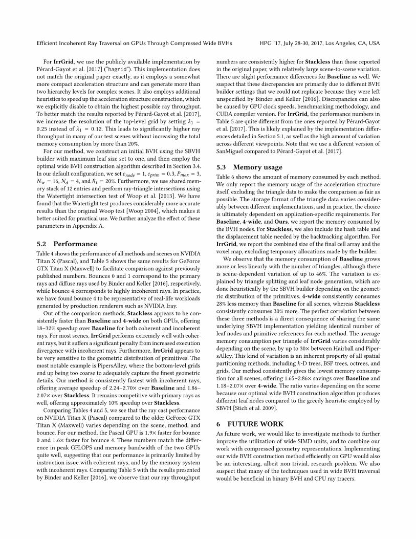
For IrrGrid, we use the publicly available implementation by

Pérard-Gayot et al. [2017] (“hagrid”). This implementation does

not match the original paper exactly, as it employs a somewhat

more compact acceleration structure and can generate more than

two hierarchy levels for complex scenes. It also employs additional

heuristics to speed up the acceleration structure construction, which

we explicitly disable to obtain the highest possible ray throughput.

To better match the results reported by Pérard-Gayot et al. [2017],

we increase the resolution of the top-level grid by setting λ1 =0.25 instead of λ1 = 0.12. This leads to significantly higher ray

throughput in many of our test scenes without increasing the total

memory consumption by more than 20%.

For our method, we construct an initial BVH using the SBVH

builder with maximum leaf size set to one, and then employ the

optimal wide BVH construction algorithm described in Section 3.4.

In our default configuration, we set cnode = 1, cprim = 0.3, Pmax = 3,

Nw = 16, Nd = 4, and Rt = 20%. Furthermore, we use shared mem-

ory stack of 12 entries and perform ray-triangle intersections using

the Watertight intersection test of Woop et al. [2013]. We have

found that the Watertight test produces considerably more accurate

results than the original Woop test [Woop 2004], which makes it

better suited for practical use. We further analyze the effect of these

parameters in Appendix A.

5.2 Performance

Table 4 shows the performance of all methods and scenes onNVIDIA

Titan X (Pascal), and Table 5 shows the same results for GeForce

GTX Titan X (Maxwell) to facilitate comparison against previously

published numbers. Bounces 0 and 1 correspond to the primary

rays and diffuse rays used by Binder and Keller [2016], respectively,

while bounce 4 corresponds to highly incoherent rays. In practice,

we have found bounce 4 to be representative of real-life workloads

generated by production renderers such as NVIDIA Iray.

Out of the comparison methods, Stackless appears to be con-

sistently faster than Baseline and 4-wide on both GPUs, offering

18–32% speedup over Baseline for both coherent and incoherent

rays. For most scenes, IrrGrid performs extremely well with coher-

ent rays, but it suffers a significant penalty from increased execution

divergence with incoherent rays. Furthermore, IrrGrid appears to

be very sensitive to the geometric distribution of primitives. The

most notable example is PipersAlley, where the bottom-level grids

end up being too coarse to adequately capture the finest geometric

details. Our method is consistently fastest with incoherent rays,

offering average speedup of 2.24–2.70× over Baseline and 1.86–

2.07× over Stackless. It remains competitive with primary rays as

well, offering approximately 10% speedup over Stackless.

Comparing Tables 4 and 5, we see that the ray cast performance

on NVIDIA Titan X (Pascal) compared to the older GeForce GTX

Titan X (Maxwell) varies depending on the scene, method, and

bounce. For our method, the Pascal GPU is 1.9× faster for bounce

0 and 1.6× faster for bounce 4. These numbers match the differ-

ence in peak GFLOPS and memory bandwidth of the two GPUs

quite well, suggesting that our performance is primarily limited by

instruction issue with coherent rays, and by the memory system

with incoherent rays. Comparing Table 5 with the results presented

by Binder and Keller [2016], we observe that our ray throughput

numbers are consistently higher for Stackless than those reported

in the original paper, with relatively large scene-to-scene variation.

There are slight performance differences for Baseline as well. We

suspect that these discrepancies are primarily due to different BVH

builder settings that we could not replicate because they were left

unspecified by Binder and Keller [2016]. Discrepancies can also

be caused by GPU clock speeds, benchmarking methodology, and

CUDA compiler version. For IrrGrid, the performance numbers in

Table 5 are quite different from the ones reported by Pérard-Gayot

et al. [2017]. This is likely explained by the implementation differ-

ences detailed in Section 5.1, as well as the high amount of variation

across different viewpoints. Note that we use a different version of

SanMiguel compared to Pérard-Gayot et al. [2017].

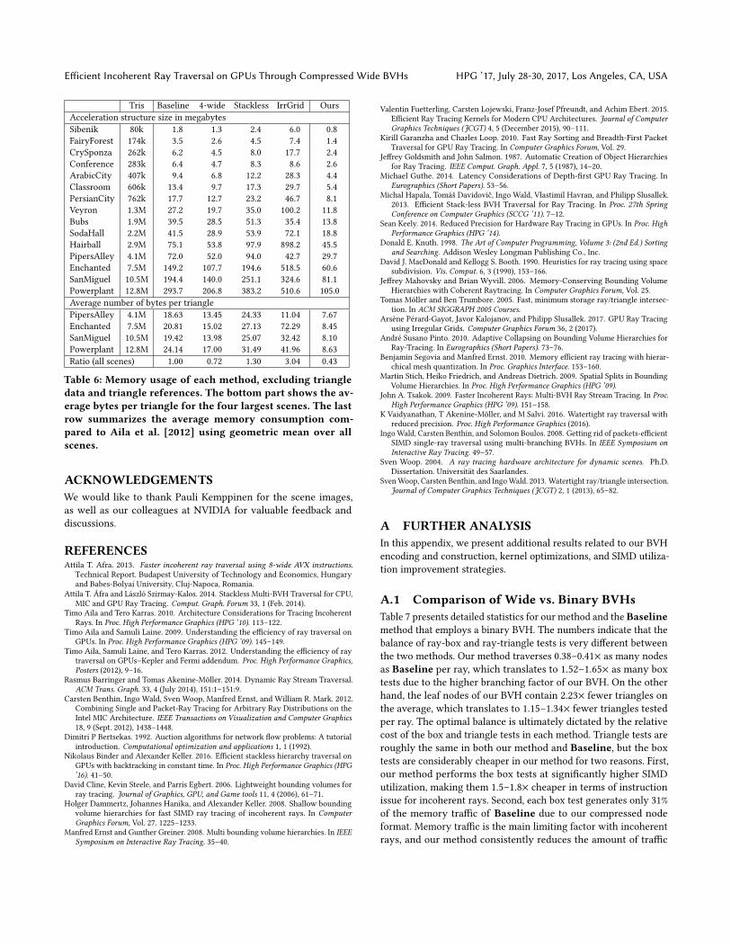
5.3 Memory usage

Table 6 shows the amount of memory consumed by each method.

We only report the memory usage of the acceleration structure

itself, excluding the triangle data to make the comparison as fair as

possible. The storage format of the triangle data varies consider-

ably between different implementations, and in practice, the choice

is ultimately dependent on application-specific requirements. For

Baseline, 4-wide, and Ours, we report the memory consumed by

the BVH nodes. For Stackless, we also include the hash table and

the displacement table needed by the backtracking algorithm. For

IrrGrid, we report the combined size of the final cell array and the

voxel map, excluding temporary allocations made by the builder.

We observe that the memory consumption of Baseline grows

more or less linearly with the number of triangles, although there

is scene-dependent variation of up to 46%. The variation is ex-

plained by triangle splitting and leaf node generation, which are

done heuristically by the SBVH builder depending on the geomet-

ric distribution of the primitives. 4-wide consistently consumes

28% less memory than Baseline for all scenes, whereas Stackless

consistently consumes 30% more. The perfect correlation between

these three methods is a direct consequence of sharing the same

underlying SBVH implementation yielding identical number of

leaf nodes and primitive references for each method. The average

memory consumption per triangle of IrrGrid varies considerably

depending on the scene, by up to 30× between Hairball and Piper-

sAlley. This kind of variation is an inherent property of all spatial

partitioning methods, including k-D trees, BSP trees, octrees, and

grids. Our method consistently gives the lowest memory consump-

tion for all scenes, offering 1.65–2.86× savings over Baseline and

1.18–2.07× over 4-wide. The ratio varies depending on the scene

because our optimal wide BVH construction algorithm produces

different leaf nodes compared to the greedy heuristic employed by

SBVH [Stich et al. 2009].

6 FUTUREWORK

As future work, we would like to investigate methods to further

improve the utilization of wide SIMD units, and to combine our

work with compressed geometry representations. Implementing

our wide BVH construction method efficiently on GPU would also

be an interesting, albeit non-trivial, research problem. We also

suspect that many of the techniques used in wide BVH traversal

would be beneficial in binary BVH and CPU ray tracers.


Sibenik1 Sibenik2 Sibenik3 Sibenik4 Sibenik5 FairyForest1 FairyForest2 FairyForest3 FairyForest4 FairyForest5 CrySponza1 CrySponza2 CrySponza3 CrySponza4 Conference1 Conference2 Conference3

Conference4 Conference5 ArabicCity1 ArabicCity2 ArabicCity3 ArabicCity4 Classroom1 PersianCity1 PersianCity2 PersianCity3 PersianCity4 Veyron1 Bubs1 Bubs2 SodaHall1 SodaHall2 SodaHall3

SodaHall4 SodaHall5 Hairball1 Hairball2 PipersAlley1 PipersAlley2 PipersAlley3 Enchanted1 Enchanted2 Enchanted3 Enchanted4 Enchanted5 SanMiguel1 SanMiguel2 SanMiguel3 Powerplant1 Powerplant2

Table 3: Test scenes used in our benchmarks. For each scene, we report an average over 1–5 viewpoints.

Baseline 4-wide Stackless IrrGrid

Ours

[Aila et al. 2012] [Guthe 2014] [Binder and Keller 2016] [Pérard-Gayot et al. 2017]

Bounce 0 1 4 0 1 4 0 1 4 0 1 4 0 1 4

Sibenik 1398 401 271 1503 1.08 448 1.12 276 1.02 1679 1.20 483 1.20 378 1.40 3143 2.25 454 1.13 224 0.83 1987 1.42 873 2.18 796 2.94

FairyForest 802 333 256 877 1.09 368 1.10 260 1.02 983 1.23 398 1.19 329 1.28 1190 1.48 317 0.95 213 0.83 1077 1.34 719 2.16 670 2.62

CrySponza 918 276 187 974 1.06 305 1.10 180 0.96 1110 1.21 349 1.26 252 1.35 2598 2.83 411 1.49 193 1.03 1163 1.27 658 2.38 557 2.98

Conference 1412 432 331 1625 1.15 488 1.13 366 1.10 1763 1.25 529 1.22 416 1.25 2483 1.76 546 1.26 342 1.03 2642 1.87 1224 2.84 1093 3.30

ArabicCity 1097 392 218 1163 1.06 436 1.11 213 0.98 1346 1.23 486 1.24 306 1.41 2271 2.07 457 1.17 184 0.84 1233 1.12 841 2.14 570 2.62

Classroom 806 294 204 938 1.16 334 1.14 194 0.95 1022 1.27 362 1.23 275 1.34 1318 1.64 285 0.97 131 0.64 1103 1.37 758 2.58 583 2.85

PersianCity 1172 409 282 1206 1.03 431 1.05 288 1.02 1374 1.17 502 1.23 384 1.36 2657 2.27 452 1.11 290 1.03 1284 1.10 741 1.81 651 2.31

Veyron 735 175 94 800 1.09 172 0.99 88 0.94 941 1.28 258 1.48 136 1.45 1514 2.06 201 1.15 84 0.89 931 1.27 435 2.49 275 2.93

Bubs 1203 403 329 1370 1.14 450 1.12 343 1.04 1537 1.28 481 1.19 374 1.14 1266 1.05 405 1.01 244 0.74 2251 1.87 1158 2.87 903 2.75

SodaHall 991 414 316 1034 1.04 454 1.10 344 1.09 1135 1.15 493 1.19 389 1.23 2801 2.83 474 1.15 332 1.05 1120 1.13 710 1.72 675 2.14

Hairball 326 86 31 376 1.15 79 0.92 28 0.92 417 1.28 115 1.34 37 1.21 496 1.52 90 1.04 36 1.17 564 1.73 244 2.84 83 2.69

PipersAlley 976 274 168 1077 1.10 306 1.12 164 0.98 1215 1.25 336 1.23 232 1.38 431 0.44 157 0.57 67 0.40 1330 1.36 732 2.67 528 3.15

Enchanted 444 83 38 487 1.10 76 0.92 35 0.92 596 1.34 114 1.38 47 1.22 766 1.73 80 0.97 39 1.03 563 1.27 204 2.47 96 2.51

SanMiguel 423 118 59 481 1.14 116 0.98 56 0.94 551 1.30 164 1.39 77 1.30 324 0.77 108 0.91 55 0.92 629 1.49 311 2.64 162 2.73

Powerplant 282 133 77 319 1.13 131 0.99 70 0.91 355 1.26 183 1.38 113 1.47 694 2.46 138 1.04 72 0.95 322 1.14 271 2.05 172 2.25

Geometric mean (all scenes) 1.10 1.06 0.98 1.24 1.27 1.32 1.64 1.04 0.87 1.36 2.36 2.70

Table 4: Performance results on NVIDIA Titan X (Pascal). The small numbers indicate raw ray throughput in millions of rays

per second (Mrays/s), and the large numbers indicate relative performance compared to Aila et al. [2012]. Bounces 0 and 1

correspond to primary rays and the first set of diffuse inter-reflection rays, respectively. The last row summarizes the average

speedup over Aila et al. [2012] using geometric mean over all scenes.

Baseline 4-wide Stackless IrrGrid

Ours

[Aila et al. 2012] [Guthe 2014] [Binder and Keller 2016] [Pérard-Gayot et al. 2017]

Bounce 0 1 4 0 1 4 0 1 4 0 1 4 0 1 4

Sibenik 761 235 169 836 1.10 280 1.19 196 1.16 893 1.17 264 1.13 214 1.27 1645 2.16 238 1.01 167 0.99 1059 1.39 469 2.00 439 2.60

FairyForest 433 197 164 487 1.12 233 1.18 187 1.14 523 1.21 219 1.11 188 1.15 632 1.46 166 0.84 143 0.87 571 1.32 391 1.98 381 2.32

CrySponza 493 165 126 539 1.09 201 1.21 138 1.09 589 1.20 194 1.18 155 1.23 1384 2.81 232 1.40 144 1.14 616 1.25 361 2.18 346 2.74

Conference 782 256 205 931 1.19 309 1.21 247 1.21 941 1.20 292 1.14 233 1.14 1490 1.91 291 1.13 211 1.03 1416 1.81 676 2.63 621 3.04

ArabicCity 595 228 145 647 1.09 271 1.19 161 1.11 717 1.21 268 1.17 185 1.28 1197 2.01 239 1.05 130 0.90 654 1.10 459 2.01 349 2.41

Classroom 440 178 140 531 1.21 223 1.25 159 1.13 549 1.25 205 1.15 170 1.21 717 1.63 170 0.95 108 0.77 589 1.34 424 2.38 428 3.05

PersianCity 632 230 171 662 1.05 258 1.12 193 1.13 729 1.15 270 1.17 216 1.26 1400 2.21 227 0.98 159 0.93 680 1.07 397 1.72 361 2.11

Veyron 400 120 75 448 1.12 135 1.13 79 1.05 501 1.25 154 1.29 105 1.39 795 1.99 141 1.18 63 0.83 494 1.23 264 2.20 187 2.47

Bubs 685 244 211 831 1.21 307 1.26 256 1.22 867 1.27 275 1.13 217 1.03 876 1.28 248 1.02 185 0.88 1218 1.78 703 2.88 579 2.75

SodaHall 529 230 181 563 1.06 267 1.16 214 1.19 601 1.14 263 1.14 210 1.16 1529 2.89 237 1.03 173 0.95 592 1.12 379 1.65 364 2.01

Hairball 181 63 28 221 1.22 68 1.07 27 0.97 226 1.25 72 1.14 32 1.17 243 1.34 65 1.03 30 1.07 300 1.66 174 2.74 67 2.44

PipersAlley 533 162 109 606 1.14 198 1.22 126 1.16 650 1.22 187 1.15 135 1.24 268 0.50 92 0.57 49 0.45 707 1.33 402 2.48 319 2.93

Enchanted 245 64 35 281 1.15 68 1.06 34 0.97 323 1.32 82 1.29 39 1.14 399 1.63 63 0.99 32 0.92 299 1.22 164 2.58 82 2.36

SanMiguel 230 79 49 273 1.19 92 1.16 51 1.03 296 1.28 100 1.26 59 1.20 199 0.87 74 0.93 47 0.95 335 1.45 223 2.82 132 2.68

Powerplant 153 92 57 176 1.15 100 1.08 58 1.03 186 1.22 110 1.19 74 1.30 352 2.30 74 0.80 53 0.93 169 1.11 165 1.78 115 2.02

Geometric mean (all scenes) 1.14 1.17 1.10 1.22 1.18 1.21 1.66 0.98 0.89 1.33 2.24 2.51

Table 5: Performance results on GeForce GTX Titan X (Maxwell). Format is the same as in Table 4 above.


Tris Baseline 4-wide Stackless IrrGrid Ours

Acceleration structure size in megabytes

Sibenik 80k 1.8 1.3 2.4 6.0 0.8

FairyForest 174k 3.5 2.6 4.5 7.4 1.4

CrySponza 262k 6.2 4.5 8.0 17.7 2.4

Conference 283k 6.4 4.7 8.3 8.6 2.6

ArabicCity 407k 9.4 6.8 12.2 28.3 4.4

Classroom 606k 13.4 9.7 17.3 29.7 5.4

PersianCity 762k 17.7 12.7 23.2 46.7 8.1

Veyron 1.3M 27.2 19.7 35.0 100.2 11.8

Bubs 1.9M 39.5 28.5 51.3 35.4 13.8

SodaHall 2.2M 41.5 28.9 53.9 72.1 18.8

Hairball 2.9M 75.1 53.8 97.9 898.2 45.5

PipersAlley 4.1M 72.0 52.0 94.0 42.7 29.7

Enchanted 7.5M 149.2 107.7 194.6 518.5 60.6

SanMiguel 10.5M 194.4 140.0 251.1 324.6 81.1

Powerplant 12.8M 293.7 206.8 383.2 510.6 105.0

Average number of bytes per triangle

PipersAlley 4.1M 18.63 13.45 24.33 11.04 7.67

Enchanted 7.5M 20.81 15.02 27.13 72.29 8.45

SanMiguel 10.5M 19.42 13.98 25.07 32.42 8.10

Powerplant 12.8M 24.14 17.00 31.49 41.96 8.63

Ratio (all scenes) 1.00 0.72 1.30 3.04 0.43

Table 6: Memory usage of each method, excluding triangle

data and triangle references. The bottom part shows the av-

erage bytes per triangle for the four largest scenes. The last

row summarizes the average memory consumption com-

pared to Aila et al. [2012] using geometric mean over all

scenes.

ACKNOWLEDGEMENTS

We would like to thank Pauli Kemppinen for the scene images,

as well as our colleagues at NVIDIA for valuable feedback and

discussions.

REFERENCES

Attila T. Afra. 2013. Faster incoherent ray traversal using 8-wide AVX instructions.Technical Report. Budapest University of Technology and Economics, Hungary

and Babes-Bolyai University, Cluj-Napoca, Romania.

Attila T. Áfra and László Szirmay-Kalos. 2014. Stackless Multi-BVH Traversal for CPU,

MIC and GPU Ray Tracing. Comput. Graph. Forum 33, 1 (Feb. 2014).

Timo Aila and Tero Karras. 2010. Architecture Considerations for Tracing Incoherent

Rays. In Proc. High Performance Graphics (HPG ’10). 113–122.Timo Aila and Samuli Laine. 2009. Understanding the efficiency of ray traversal on

GPUs. In Proc. High Performance Graphics (HPG ’09). 145–149.Timo Aila, Samuli Laine, and Tero Karras. 2012. Understanding the efficiency of ray

traversal on GPUs–Kepler and Fermi addendum. Proc. High Performance Graphics,Posters (2012), 9–16.

Rasmus Barringer and Tomas Akenine-Möller. 2014. Dynamic Ray Stream Traversal.

ACM Trans. Graph. 33, 4 (July 2014), 151:1–151:9.

Carsten Benthin, Ingo Wald, Sven Woop, Manfred Ernst, and William R. Mark. 2012.

Combining Single and Packet-Ray Tracing for Arbitrary Ray Distributions on the

Intel MIC Architecture. IEEE Transactions on Visualization and Computer Graphics18, 9 (Sept. 2012), 1438–1448.

Dimitri P Bertsekas. 1992. Auction algorithms for network flow problems: A tutorial

introduction. Computational optimization and applications 1, 1 (1992).Nikolaus Binder and Alexander Keller. 2016. Efficient stackless hierarchy traversal on

GPUs with backtracking in constant time. In Proc. High Performance Graphics (HPG’16). 41–50.

David Cline, Kevin Steele, and Parris Egbert. 2006. Lightweight bounding volumes for

ray tracing. Journal of Graphics, GPU, and Game tools 11, 4 (2006), 61–71.Holger Dammertz, Johannes Hanika, and Alexander Keller. 2008. Shallow bounding

volume hierarchies for fast SIMD ray tracing of incoherent rays. In ComputerGraphics Forum, Vol. 27. 1225–1233.

Manfred Ernst and Gunther Greiner. 2008. Multi bounding volume hierarchies. In IEEESymposium on Interactive Ray Tracing. 35–40.

Valentin Fuetterling, Carsten Lojewski, Franz-Josef Pfreundt, and Achim Ebert. 2015.

Efficient Ray Tracing Kernels for Modern CPU Architectures. Journal of ComputerGraphics Techniques (JCGT) 4, 5 (December 2015), 90–111.

Kirill Garanzha and Charles Loop. 2010. Fast Ray Sorting and Breadth-First Packet

Traversal for GPU Ray Tracing. In Computer Graphics Forum, Vol. 29.

Jeffrey Goldsmith and John Salmon. 1987. Automatic Creation of Object Hierarchies

for Ray Tracing. IEEE Comput. Graph. Appl. 7, 5 (1987), 14–20.Michael Guthe. 2014. Latency Considerations of Depth-first GPU Ray Tracing. In

Eurographics (Short Papers). 53–56.Michal Hapala, Tomáš Davidovič, Ingo Wald, Vlastimil Havran, and Philipp Slusallek.

2013. Efficient Stack-less BVH Traversal for Ray Tracing. In Proc. 27th SpringConference on Computer Graphics (SCCG ’11). 7–12.

Sean Keely. 2014. Reduced Precision for Hardware Ray Tracing in GPUs. In Proc. HighPerformance Graphics (HPG ’14).

Donald E. Knuth. 1998. The Art of Computer Programming, Volume 3: (2nd Ed.) Sortingand Searching. Addison Wesley Longman Publishing Co., Inc.

David J. MacDonald and Kellogg S. Booth. 1990. Heuristics for ray tracing using space

subdivision. Vis. Comput. 6, 3 (1990), 153–166.Jeffrey Mahovsky and Brian Wyvill. 2006. Memory-Conserving Bounding Volume

Hierarchies with Coherent Raytracing. In Computer Graphics Forum, Vol. 25.

Tomas Möller and Ben Trumbore. 2005. Fast, minimum storage ray/triangle intersec-

tion. In ACM SIGGRAPH 2005 Courses.Arsène Pérard-Gayot, Javor Kalojanov, and Philipp Slusallek. 2017. GPU Ray Tracing

using Irregular Grids. Computer Graphics Forum 36, 2 (2017).

André Susano Pinto. 2010. Adaptive Collapsing on Bounding Volume Hierarchies for

Ray-Tracing. In Eurographics (Short Papers). 73–76.Benjamin Segovia and Manfred Ernst. 2010. Memory efficient ray tracing with hierar-

chical mesh quantization. In Proc. Graphics Interface. 153–160.Martin Stich, Heiko Friedrich, and Andreas Dietrich. 2009. Spatial Splits in Bounding

Volume Hierarchies. In Proc. High Performance Graphics (HPG ’09).John A. Tsakok. 2009. Faster Incoherent Rays: Multi-BVH Ray Stream Tracing. In Proc.

High Performance Graphics (HPG ’09). 151–158.K Vaidyanathan, T Akenine-Möller, and M Salvi. 2016. Watertight ray traversal with

reduced precision. Proc. High Performance Graphics (2016).IngoWald, Carsten Benthin, and Solomon Boulos. 2008. Getting rid of packets-efficient

SIMD single-ray traversal using multi-branching BVHs. In IEEE Symposium onInteractive Ray Tracing. 49–57.

Sven Woop. 2004. A ray tracing hardware architecture for dynamic scenes. Ph.D.

Dissertation. Universität des Saarlandes.

SvenWoop, Carsten Benthin, and IngoWald. 2013. Watertight ray/triangle intersection.

Journal of Computer Graphics Techniques (JCGT) 2, 1 (2013), 65–82.

A FURTHER ANALYSIS

In this appendix, we present additional results related to our BVH

encoding and construction, kernel optimizations, and SIMD utiliza-

tion improvement strategies.

A.1 Comparison of Wide vs. Binary BVHs

Table 7 presents detailed statistics for our method and the Baseline

method that employs a binary BVH. The numbers indicate that the

balance of ray-box and ray-triangle tests is very different between

the two methods. Our method traverses 0.38–0.41× as many nodes

as Baseline per ray, which translates to 1.52–1.65× as many box

tests due to the higher branching factor of our BVH. On the other

hand, the leaf nodes of our BVH contain 2.23× fewer triangles on

the average, which translates to 1.15–1.34× fewer triangles tested

per ray. The optimal balance is ultimately dictated by the relative

cost of the box and triangle tests in each method. Triangle tests are

roughly the same in both our method and Baseline, but the box

tests are considerably cheaper in our method for two reasons. First,

our method performs the box tests at significantly higher SIMD

utilization, making them 1.5–1.8× cheaper in terms of instruction

issue for incoherent rays. Second, each box test generates only 31%

of the memory traffic of Baseline due to our compressed node

format. Memory traffic is the main limiting factor with incoherent

rays, and our method consistently reduces the amount of traffic


Baseline Ours

Bounce 0 1 4 0 1 4

Ray-node tests 35.63 39.32 38.48 14.69 14.95 15.02

Ray-triangle tests 7.58 10.66 11.93 6.59 7.98 9.03

Main loop iterations 2.29 2.28 2.29 15.45 17.40 17.54

Children per node 2.00 2.00 2.00 7.51 7.51 7.51

Triangles per leaf 3.48 3.48 3.48 1.56 1.56 1.56

Reference duplication 1.24 1.24 1.24 1.24 1.24 1.24

Node bytes fetched 2281 2516 2463 1176 1196 1202

Triangle bytes fetched 461 642 718 316 383 434

Total bytes fetched 2741 3159 3181 1492 1579 1636

Node test SIMD util. 88% 47% 40% 88% 72% 71%

Triangle test SIMD util. 64% 24% 22% 52% 25% 24%

Ray init SIMD util. 98% 92% 89% 82% 42% 41%

Table 7: Comparison of intersection test counts, BVH statis-

tics, memory traffic for nodes and triangles, and SIMD uti-

lization between ourmethod andAila et al. [2012]. The num-

bers represent arithmeticmeans over our test scenes, exclud-

ing Powerplant.

Mrays/s for bounce BVH statistics

0 1 4 nodes tris/leaf child/node

Node collapsing method

Optimal SAH ⋆ 100.0% 100.0% 100.0% 100% 1.56 7.51

Afra et al. [2013] 96.0% 99.0% 97.2% 152% 1.24 6.39

Wald et al. [2008] 93.6% 93.6% 91.7% 138% 2.21 4.34

Fixed depth 93.1% 92.8% 90.8% 154% 2.21 3.99

Child slot assignment

Auction method ⋆ 100.0% 100.0% 100.0% 100% 1.56 7.51

Greedy selection 99.8% 99.0% 98.8% 100% 1.56 7.51

Random order 78.7% 71.6% 72.7% 100% 1.56 7.51

SAH cost parameters (cnode = 1.0)

cprim = 0.0 97.2% 95.5% 94.0% 95% 1.90 6.66

cprim = 0.1 98.0% 98.0% 97.6% 95% 1.66 7.43

cprim = 0.2 99.3% 99.1% 98.8% 97% 1.62 7.48

cprim = 0.3 ⋆ 100.0% 100.0% 100.0% 100% 1.56 7.51

cprim = 0.4 100.2% 100.8% 100.2% 104% 1.51 7.49

cprim = 0.5 99.6% 101.2% 100.7% 109% 1.45 7.45

cprim = 1.0 99.4% 102.0% 101.8% 130% 1.28 7.13

Table 8: Effect of wide BVH construction. Mrays/s and the

number of BVH nodes are expressed relative to our default

configuration, indicated by⋆, using geometricmean over all

scenes. The last two columns summarize triangles per leaf

and children per internal node using arithmetic mean over

the scenes.

resulting from node and triangle fetches by about 2× compared to

Baseline.

A.2 Wide BVH Construction

Table 8 evaluates different ways of constructing the wide BVH. We

compare our optimal node collapsing method to the greedy surface

area-based heuristics of Afra et al. [2013] and Wald et al. [2008], as

well as simply collapsing each k consecutive levels of the binary

BVH [Ernst and Greiner 2008]. The results are favorable to our

method in terms of both performance (1–10% faster) and memory

usage (1.38–1.54× smaller). Wald et al. [2008] retain the original

leaf nodes of the binary BVH as is, while Afra et al. [2013] split the

leaves as long as there are unused child slots in their respective

Bounce 0 1 4 8

SIMD utilization checks

Both enabled ⋆ 100.0% 100.0% 100.0% 100.0%

No dynamic fetch 105.3% 76.3% 83.0% 86.7%

No tri postponing 104.3% 74.6% 79.9% 82.3%

Both disabled 105.7% 48.0% 54.2% 57.8%

Shared memory stack

Disabled 97.5% 76.2% 71.5% 71.7%

2 entries 97.4% 83.6% 80.3% 80.2%

4 entries 98.9% 91.9% 90.5% 90.5%

6 entries 99.9% 98.1% 97.9% 97.8%

8 entries 99.9% 99.8% 99.8% 100.2%

12 entries ⋆ 100.0% 100.0% 100.0% 100.0%

16 entries 91.7% 90.8% 93.6% 95.0%

Ray-triangle test

Watertight ⋆ 100.0% 100.0% 100.0% 100.0%

Möller-Trumbore 103.2% 103.2% 102.0% 101.7%

Woop 105.7% 102.6% 98.2% 97.6%

Table 9: Performance effect of various optimizations and im-

plementation choices. The numbers represent the relative

performance with respect to our default configuration, indi-

cated by ⋆, using geometric mean over all scenes.

parent nodes. The former leads to low child slot utilization, while

the latter leads to low number of triangles per leaf. By constructing

the internal nodes and leaf nodes in a single joint optimization pass,

our method is able to reach high child slot utilization while keeping

the leaves reasonably large.

We also compare the auction method [Bertsekas 1992] for child

node ordering to a greedy approach, as well as to purely random

ordering. The greedy variant constructs the same 8 × 8 cost table

as the auction method and performs one assignment by finding the

cell with the lowest cost. It then removes the corresponding row

and column from the table and repeats the process until all children

have been assigned. The results show that both methods offer a

significant improvement over random ordering (27–40%). Although

the greedy method is inferior in theory, it is pretty much on par

with the auction method in practice.

The bottom section of Table 8 shows the effect of the SAH cost

parameters. The absolute magnitude of the parameters is irrelevant,

so we set cnode = 1 and sweep over the value of cprim. In effect, cprimcontrols the average number of triangles per leaf, offering a tradeoff

between performance and memory consumption. Increasing cprimreduces ray-triangle tests by making the leaves smaller, while de-

creasing it reduces the number of BVH nodes by making the leaves

larger. cprim = 0.3 represents a sweet spot where we get 98% of the

performance at only 5% additional memory. Interestingly, the same

value also leads to the highest average child slot utilization. We did

not experiment with different choices for Pmax , because our data

structures only support Pmax ≤ 3.

A.3 Kernel Optimizations

Table 9 analyzes the performance of various optimizations and

implementation choices. Dynamic ray fetching and triangle post-

poning have a significant positive impact on the performance of

incoherent rays. On the other hand, these optimizations slow down


coherent rays, but the effect is fairly small (4–6%). The increased

SIMD utilization benefits bounce 1 more than bounce 4, because

the latter is primarily limited by the memory system and is thus

less sensitive to SIMD effects. Storing parts of the traversal stack in

shared memory is always a net win, and it is especially beneficial for

highly incoherent rays due to the reduced external memory traffic.

We can increase the number of entries to 12 with no negative effects,

but at 13 entries the occupancy of our kernel becomes limited by

shared memory, leading to decreased performance. Interestingly,

we obtain virtually all of the benefits with only 8 entries, i.e., 64

bytes of shared memory per thread.

The bottom section of Table 9 shows the performance of different

ray-triangle tests. In our benchmarks, we store the triangles in the

same order in memory as they appear in the BVH, along with their

corresponding indices in the original model. For Watertight [Woop

et al. 2013] and Möller-Trumbore [Möller and Trumbore 2005], we

have 40 bytes of data per triangle that we pad to 48 bytes in order to

better match the comparison methods. For Woop test [Woop 2004],

the preprocessing phase already produces 48 bytes per triangle, so

we have to place the original triangle index in a separate array that

we consult after tracing each ray. As expected, the Watertight test

is slightly more expensive than the other two, but we feel that the

difference is not significant enough to offset the practical benefits

of increased numerical accuracy. Interestingly, the performance of

the Woop test drops considerably with highly incoherent rays due

to the additional triangle index lookup.

A.4 SIMD Utilization

Table 10 analyzes the different dynamic ray fetching and triangle

postponing strategies in detail. Dynamic fetching aims to improve

the SIMD utilization of the node and triangle tests at the cost of

reduced SIMD utilization during ray initialization. The original

heuristic of Aila and Laine [2009] exhibits an inherent conflict

between coherent and incoherent rays: for bounce 0, the optimal

choice is to disable dynamic fetching altogether, but for bounce

4, it is highly beneficial to employ aggressive dynamic fetching

with Nt = 8. Our improved heuristic adapts to the ray distribution

automatically, reaching optimal performance for both coherent and

incoherent rays with no manual tuning. As can be seen in the table,

our heuristic is fairly insensitive to the exact choice of Nw and Nd .

We chose our default configuration to yield the highest performance

across all different bounces and test scenes. Triangle postponing

aims to improve the SIMD utilization of the triangle tests at the

cost of reduced SIMD utilization of the node tests. The optimal

balance is tightly connected to the choice of cprim, as discussed in

the context of Tables 7 and 8.

Mrays/s Node test Tri test Ray init

Bounce 0 4 0 4 0 4 0 4

Original heuristic – inactive thread threshold

Nt = 0 78% 94% 89% 84% 37% 29% 17% 8%

Nt = 8 92% 100% 89% 75% 44% 25% 50% 32%

Nt = 16 95% 99% 83% 66% 54% 22% 84% 56%

Nt = 24 100% 96% 87% 60% 56% 19% 93% 80%

Nt = 32 106% 83% 85% 42% 57% 14% 100% 100%

Improved heuristic – lost work threshold

Nw = 0 99% 101% 88% 77% 51% 26% 70% 26%

Nw = 8 100% 100% 88% 73% 52% 25% 77% 35%

Nw = 16 ⋆ 100% 100% 87% 71% 52% 24% 81% 41%

Nw = 24 100% 100% 87% 69% 53% 23% 85% 45%

Nw = 32 100% 99% 87% 68% 53% 23% 87% 49%

Nw = 64 100% 97% 86% 64% 53% 21% 93% 62%

Improved heuristic – decrement parameter

Nd = 0 92% 100% 89% 77% 44% 26% 45% 26%

Nd = 4 ⋆ 100% 100% 87% 71% 52% 24% 81% 41%

Nd = 8 100% 98% 85% 64% 53% 21% 98% 66%

Triangle postponing threshold

Rt = 0% 105% 80% 94% 82% 44% 9% 91% 42%

Rt = 10% 102% 95% 91% 77% 48% 16% 88% 41%

Rt = 20% ⋆ 100% 100% 87% 71% 52% 24% 81% 41%

Rt = 50% 92% 97% 75% 52% 64% 45% 71% 40%

Rt = 100% 58% 52% 46% 15% 83% 80% 68% 37%

Table 10: SIMD utilization. The columns show relative per-

formance wrt. our default configuration, indicated by ⋆, as

well as the average SIMD utilization in different parts of our

traversal kernel.We use geometricmean over the test scenes

for the Mrays/s, and arithmetic mean for SIMD utilization.

efficient incoherent ray traversal on gpus through...

Documents