efficient vehicle tracking and classification for an ...ambardek/_includes/thesiscs.pdf ·...
TRANSCRIPT

University of Nevada Reno
Efficient Vehicle Tracking and Classification for an Automated Traffic
Surveillance System
A thesis submitted in partial fulfillment of the requirements for the degree of Master of Science
in Computer Science
by
Amol A. Ambardekar
Dr. Mircea Nicolescu, Thesis Advisor
December, 2007

We recommend that the thesis prepared under our supervision by
AMOL A. AMBARDEKAR
entitled
Efficient Vehicle Tracking and Classification
for an Automated Traffic Surveillance System
be accepted in partial fulfillment of the requirements for the degree of
MASTER OF SCIENCE
Mircea Nicolescu, Ph.D., Advisor
George Bebis, Ph.D., Committee Member
Monica Nicolescu, Ph.D., Committee Member
Mark Pinsky, Ph.D., Graduate School Representative
Marsha H. Read, Ph. D., Associate Dean, Graduate School
December, 2007
THE GRADUATE SCHOOL

i
Abstract
As digital cameras and powerful computers have become wide spread, the number
of applications using vision techniques has increased enormously. One such application
that has received significant attention from the computer vision community is traffic
surveillance. We propose a new traffic surveillance system that works without prior,
explicit camera calibration, and has the ability to perform surveillance tasks in real time.
Camera intrinsic parameters and its position with respect to the ground plane were
derived using geometric primitives common to any traffic scene. We use optical flow and
knowledge of camera parameters to detect the pose of a vehicle in the 3D world. This
information is used in a model-based vehicle detection and classification technique
employed by our traffic surveillance application. The object (vehicle) classification uses
two new techniques − color contour based matching and gradient based matching. We
report good results for vehicle detection, tracking, and vehicle speed estimation. Vehicle
classification results can still be improved, but the approach itself gives thoughtful insight
and direction to future work that would result in a full fledged traffic surveillance system.

ii
Dedication
This work is dedicated to my family: my parents Ashok and Sanjivani, my sister
Ashvini and my brother Amit. I would not be here without you and your help. I am
eternally thankful to you for your love and support.

iii
Acknowledgments
I would like to take this opportunity to thank my advisor Dr. Mircea Nicolescu for
his advice and encouragement. This work would not have been possible without his help,
direction and especially his patience, when I took longer than expected to finish things.
Thanks to Dr. George Bebis, Dr. Monica Nicolescu and Dr. Mark Pinsky for
accepting to serve on my thesis committee.
I would also like to thank all my colleagues in Computer Vision Lab.
iv
Table of Contents
Abstract i
Dedication ii
Acknowledgements iii
Table of Contents iv
List of Tables vi
List of Figures vii
1. Introduction 1
2. Previous Work 3
2.1 Foreground Object Detection ..………..………………………………………....3
2.2 Camera Calibration ……………………………………………………………....8
2.3 Video Surveillance................................................................................................10
2.4 Vehicle Detection and Classification ...................................................................12
2.5 Vehicle Tracking ……………………………………………………………….16
3. Overview 21
4. Description of Our Approach 24
4.1 Camera Calibration and Synthetic Camera Modeling……..................................24
4.2 Background Modeling and Foreground Object Detection…................................31
4.3 Vehicle Pose Estimation Using Optical Flow......................................................36
4.4 Reconstruction Using Synthetic Camera ……………………………………….39
4.5 Vehicle Detection and Classification …………………………………………...39
4.6 Vehicle Tracking and Traffic Parameter Collection ……………………………45

v
5. Experimental Results 47
6. Conclusions and Future Work 54
6.1 Discussion ............................................................................................................54
6.2 Directions of Future Work ...................................................................................56
References 58

vi
List of Tables
4.1 Matching score description .........................................................................................43
5.1 Quantitative Results for the VS video sequence .........................................................52
5.2 Quantitative Results for the SS video sequence .........................................................53

vii
List of Figures
2.1 Foreground object detection..........................................................................................3
3.1 Traffic video surveillance system overview ...............................................................21
4.1 Geometric primitives………………………………………………………………...25
4.2 Graphical representation of the vanishing points and a vanishing line …………......26
4.3 World and camera coordinate system…………………………………………….....28
4.4 Geometrical representation of synthetic camera parameters………………………...30
4.5 Background modeling and foreground object detection algorithm……………….....32
4.6 An example of traffic scene and its corresponding ROI template…………………...33
4.7 Pixel classification into foreground and background………………………………...35
4.8 An example of detected foreground………………………………………………….36
4.9 Algorithm for vehicle pose estimation using optical flow…………………………...37
4.10 Average optical flow vectors ………………………………………………………38
4.11 3D wire-frame models……………………………………………………………...39
4.12 Detected edges of a vehicle ………………………………………………………...41
4.13 Algorithm for vehicle detection and classification ………………………………...41
4.14 Color contour templates and matching templates .....................................................42
4.15 Algorithm for vehicle tracking...................................................................................45
5.1 Models overlapped onto actual vehicles (VS) ............................................................47
5.2 Models overlapped onto actual vehicles (VS) ............................................................48
5.3 Vehicle tracking (VS) .................................................................................................48
5.4 Vehicle tracking (SS) ..................................................................................................49

viii
5.5 Vehicle tracking failure (VS) ......................................................................................50
5.6 Traffic surveillance – snapshot from VS ....................................................................51

1
Chapter 1. Introduction The rapidly increasing capacity of digital storage, computation power and the
recent innovations in video compression standards [1] lead to a strong growth of
available video content. Digital cameras, which were novelty items in the 80’s, have
become ubiquitous in the last two decades. This has led to cheaper and better video
surveillance systems. The video data stored by these systems needs to be analyzed, which
is generally done by humans on need-to-know basis (e.g., as a forensic tool after a bank
robbery). This undermines the ability of video surveillance as an active real time
observer. Video Content Analysis (VCA) algorithms address this problem. For video
surveillance, this technology can be used to effectively assist security personnel. State-of-
the-art VCA systems comprise object detection and tracking, thereby generating location
data of key objects in the video imagery of each camera. Classification of the detected
objects is commonly done using the size of the object, where simple camera calibration is
applied to compensate for the perspective.
Visual traffic surveillance has attracted significant interest in computer vision,
because of its tremendous application prospect. Efficient and robust localization of
vehicles from an image sequence (video) can lead to semantic results, such as “Car No. 3
stopped,” “Car No. 4 is moving faster than car No. 6.” However, such information can
not be retrieved from image sequences as easily as humans do. For any video surveillance
problem, effective segmentation of foreground (region of interest in image) and
background plays a key role in subsequent detection, classification and tracking results. A
traffic surveillance system needs to detect vehicles and classify them if possible.

2
Generating vehicle trajectories from video data is also an important application and can
be used in analyzing traffic flow parameters for ATMS (Advanced Transportation
Management Systems) [2]. Information such as gap, headway, stopped-vehicle detection,
speeding vehicle, and wrong-way vehicle alarms can be useful for Intelligent
Transportation Systems [3].
The rest of this thesis is organized as follows. Chapter 2 discusses the previous
work related to different video surveillance systems and their components. Chapter 3
gives an overview of our approach for a traffic surveillance system. In chapter 4, we give
implementation details. Experimental results of the proposed technique are presented in
Chapter 5. Chapter 6 discusses the conclusions and presents future directions of work.

3
Chapter 2. Previous Work 2.1 Foreground Object Detection Foreground object detection is the backbone of most video surveillance
applications. Foreground object detection is mainly concerned with detecting objects of
interest in an image sequence. Fig. 2.1 shows an example of foreground object detection.
Fig. 2.1(a) is the original image and Fig. 2.1(b) is the detected foreground using the
algorithm discussed in [4].
(a) (b)
Fig. 2.1 Foreground object detection using the algorithm discussed in [4]. (a) Original Image
(b) Foreground detected shown in white
As shown in Fig. 2.1, not everything we want to be detected as foreground is
detected. If we slightly modify the parameters, we might be able to get more objects
detected, but this would also increase false positives due to quasi-stationary backgrounds
such as waving trees, rain, snow, and artifacts due to specular reflection. There is also a
problem of shadows for outdoor scenes. Researchers have developed many methods to
deal with foreground object detection. The simplest one is taking consecutive frame

4
difference. It works well when the background is stationary, which is not the case of
video surveillance.
In one of the earliest research efforts [15] the foreground object is detected by
subtracting the current picture from the stored background picture, and then applying a
threshold to the resulting difference image. The method obviously fails if the background
is dynamic. Recently, it has become popular to model the pixel-wise color distribution of
the background through statistical methods. Parametric methods for example assume a
parametric model for each pixel in the image, and then try to classify it as foreground or
background using this model. The simplest one of these approaches is assuming Gaussian
probability distribution for each pixel [7, 12]. Then, this model (mean and variance) is
updated with the pixel values from the new images (frames) in the image sequence
(video). After the model has accrued enough information (generally after few frames), the
decision is made for each pixel. If a pixel (x,y) satisfies
)),((),(),( yxStdCyxMeanyxI ×<− (2.1)
where I(x,y) is pixel intensity, C is a constant, Mean(x,y) is the mean, Std(x,y) is the
standard deviation, it is marked as background pixel. If it does not satisfy (2.1), it is
marked as foreground pixel.
A single 3D Gaussian model for each pixel in the scene is built in [7], where the
mean and covariance of the model were learned in each frame. These methods that
employ a single Gaussian work well when the background is relatively stationary.
However, the task becomes difficult when the background contains shadows and moving
objects (e.g., wavering tree branches). The probability distribution of such background
can not be captured using a single Gaussian.

5
This obviously led researchers to methods that use more than one Gaussian
(Mixture of Gaussians (MoG)) to address the multi-modality of the underlying
background [5, 6]. In MoG, the colors from a pixel in a background object are described
by multiple Gaussian distributions. Good foreground object detection results were
reported by applying MoG to outdoor scenes. Further investigations showed that MoG
with more than two Gaussians can degrade the performance in foreground object
detection [8, 9]. There was also a problem of determining number of Gaussians to be
used to get optimal results.
The background variation model employed in W4 [10] is a generalization of the
Gaussian model. In [11], Toyama et al. employed a linear Wiener filter to learn and
predict color changes in each background pixel through the video. The linear predictor
can model both stationary and moving background objects. The weakness of this method
is that it is difficult to model non-periodical background changes.
In methods that explicitly model the background density estimation, foreground
detection is performed by comparing the estimated probabilities of each pixel with a
global threshold or local thresholds. Also, in these methods, there are several parameters
that need to be estimated from the data to achieve accurate density estimation for
background. However, most of the times this information is not known beforehand.
Non-parametric methods do not assume any fixed model for probability
distribution of background pixels. In [3], Li et al. proposed a novel method using a
general Bayesian framework which can integrate multiple features to model the
background for foreground object detection. However, it is prone to absorb foreground
objects if they are motionless for a long time. Also, parameter selection plays a big role in

6
getting optimal results for a set of image sequences. El Gammal et al. proposed a non-
parametric kernel density estimation for pixel-wise background modeling without making
any assumption on its probability distribution [13]. This method is known to deal with
multimodality in background pixel distributions without determining the number of
modes in the background. In order to adapt the model a sliding window is used in [14].
However the model convergence is critical in situations where the illumination suddenly
changes. Kim et al. in [29] proposed a layered modeling technique in order to update the
background for scene changes. Tavakkoli et al. proposed a new approach for foreground
region detection using robust recursive learning in [20]. In [26], support vector machines
were used to recover a background estimate that can be used to classify the pixels into
foreground and background. Since no sample of foreground regions is present in the
training steps of this approach, it explicitly addresses the single-class classification
problem in foreground region detection.
Kalman filters have also been used to perform foreground object detection. In
[16], each pixel is modeled using a Kalman filter. In [21], a robust Kalman filter is used
in tracking explicit curves. A robust Kalman filter framework for the recovery of moving
objects’ appearance is proposed in [22]. However, the framework does not model
dynamic, textured backgrounds.
All these methods address the problem of segmentation given a dynamic
background. However, they do not take advantage of inter-pixel correlation and global
appearance. In [17], Hsu et al. use region-based features (e.g., block correlation) to detect
foreground object(s). Change detection between consecutive frames is achieved via block

7
matching; thus, the foreground object(s) can only be detected at a coarse scale unless a
multi-scale based approach is used.
If a stereo camera is used, depth information can be recovered from the scene.
Background subtraction methods that rely only on depth are used in [18]. These methods
may turn out to be unreliable when the foreground objects are too close to the
background. Combined use of depth and color is proposed in [19]. However, the
approach assumes the background scene is relatively static. In addition, only indoor
experimental testing was reported.
Motion-based approaches have also been proposed. Some researchers utilized the
optical flow to solve this problem [23, 24]. The optical flow model is effective on small
moving objects. In [25], Wixson proposed an algorithm to detect salient motion by
integrating frame-to-frame optical flow over time; thus, it is possible to predict the
motion pattern of each pixel. The saliency measure is then computed to detect the object
locations. This approach assumes that the object tends to move in a consistent direction
over time, and that foreground motion has different saliency. This algorithm may fail
when there is no obvious difference between the motion fields of the foreground and
background. In general, there are some drawbacks of using motion as a foreground object
detector: calculation of optical flow consumes too much time and the inner points of a
large homogeneous object (e.g. a car with single color) can not be featured with the
optical flow.
Some approaches exploit spatio-temporal intensity variation. For instance [27, 28]
employ analysis of XT or YT video slices. By detecting the translational blobs in these
slices, it is possible to detect and track walking people and recognize their gait. If both

8
foreground and background objects exhibit periodic motion, the method may perform
inaccurately.
2.2 Camera Calibration
From a mathematical point of view, an image is a projection of a three
dimensional space onto a two dimensional space. Geometric camera calibration is the
process of determining the 2D-3D mapping between the camera and the world coordinate
system [30]. Therefore, obtaining the 3D structure of a scene depends critically on having
an accurate camera model. In the case of a simple pin-hole camera, 6 extrinsic (the
position and orientation of camera in some world coordinate system) and 4 intrinsic
parameters (principal point, focal length and aspect ratio) describe full camera
calibration.
Much work has been done, starting in the photogrammetry community and more
recently in computer vision. We can classify those techniques roughly into two
categories: photogrammetric calibration and self-calibration. In photogrammetric
calibration approaches, calibration is performed by observing a calibration object whose
geometry in 3D space is known with very good precision. Calibration can be done very
efficiently using this approach [46]. Self-calibration techniques do not use any calibration
object. A camera is moved in a static scene and images are taken with fixed internal
parameters; the rigidity of the scene provides sufficient information to recover calibration
parameters [47].
Initial efforts in camera calibration employed full-scale non-linear optimization to
do camera calibration [31, 32, 33]. It allows easy adaptation of any arbitrarily complex

9
yet accurate model for imaging. Faig’s method is a good representative of these methods
[32]. High accuracy could be achieved using these methods, but they require a good
initial guess and a computationally intensive non-linear search. Direct Linear
Transformation (DLT), developed by Abdel-Aziz et al. required only linear equations to
be solved [34]. However, it was later found that, unless lens distortion is ignored, full
scale non-linear search is needed.
Although the equations governing the transformation from 3D world coordinates
to 2D image coordinates are nonlinear functions of intrinsic and extrinsic camera
parameters, they are linear if lens distortion is ignored. This information made it possible
to compute a perspective transformation matrix first using linear equations [35, 36, 37].
The main advantage of these methods is that they eliminate nonlinear optimization.
However, lens distortion can not be modeled using these methods and the number of
unknowns in linear equations is generally much larger than the actual degrees of freedom.
Other methods such as two-plane methods [38, 39] and geometric techniques [40] have
also been employed.
The calibration model [41] presented by Tsai was the first camera calibration
model that included radial geometric distortion, yet using linear computation methods
and coplanar groups of points for calibration. However, it is constrained by having an
incidence angle of at least 30 degrees. Batista et al. presented a new method that does not
have such restriction [42].
If images are taken by the same camera with fixed internal parameters,
correspondences between three images are sufficient to recover both the internal and
external parameters which allow us to reconstruct 3D structure up to a similarity [48, 49].

10
Traditionally, the structure-from-motion problem used low-level geometric entities (or
features) such as points and lines with hardly any geometric constraints. Although
theoretically sound, these methods suffer from two main disadvantages. First, they
usually require a large number of features to achieve robustness; and second, because
there are no constraints among the features, errors in localizing these features in the
image propagate to the structure unnoticed [50].
Sturm et al. introduced a general algorithm for plane-based calibration that can
deal with an arbitrary number of views and calibration planes [43]. Worrall et al.
presented an interactive tool for calibrating a camera that is suitable for use in outdoor
scenes [44]. They used this interactive tool to calibrate traffic scenes with acceptable
accuracy. In [45], Wang et al. presented a camera calibration approach using vanishing
lines. Masoud et al. presented a method that uses certain geometric primitives commonly
found in traffic scenes in order to recover calibration parameters [50].
2.3 Video Surveillance
Video surveillance applications are interested in the real-time observation of
humans or vehicles in some environment (indoor, outdoor, or aerial), leading to a
description of the activities of the objects within the environment. A complete video
surveillance system typically consists of foreground segmentation, object detection,
object tracking, human or object analysis, and activity analysis. There are different
approaches suggested in the literature for video surveillance. This section presents an
overview of some of the most important approaches.

11
Pfinder [7] (developed by MIT Media Lab) has evolved over several years and
has been used to track a person in a large room size space. It uses a multi-class statistical
model of color and shape to obtain a 2D representation of head and hands in a wide range
of viewing conditions. Pfinder has been successfully used in many applications. In
Spfinder [52] which is an extension of Pfinder, a wide baseline stereo camera is used to
obtain 3D models. Spfinder has been used in a smaller desk-area environment to capture
accurate 3D movements of head and hands.
KidRooms [53] is a tracking system based on “closed world regions.” These are
regions of space and time in which the specific context of what is in the regions is known.
These regions are tracked in real-time domains where object motions are not smooth or
rigid and where multiple objects are interacting. It was one of the first multi-person, fully
automated, interactive, narrative environment ever constructed using non-encumbering
sensors. Rehg et al. developed Smart Kiosk [54] to detect and track people in front of a
kiosk. It uses both color information, face detection, and stereo information for detection.
However, when people are very close to the kiosk, it can only track a single person.
Olson et al. developed a general purpose system [55] for moving object detection and
event recognition. They detected moving objects using change detection and tracked
them using first-order prediction and nearest-neighbor matching. It is designed for indoor
surveillance and it cannot handle small motions of background objects. It is a single
person tracking system.
CMU developed a distributed system that allows a human operator to monitor
activities over a large area using a distributed network of active video sensors [56]. Their
system detects moving targets using the pixelwise difference between consecutive image

12
frames. A classification metric is applied to these targets to classify them into categories
such as human, human group, car, and truck using shape and color analysis, and these
labels are used to improve tracking using temporal consistency constraints. MIT's system
[58], [59] uses a distributed set of sensors, and adaptive tracking to calibrate distributed
sensors, classify detected objects, learn common patterns of activity for different object
classes, and detect unusual activities. W4 [10] employs a combination of shape analysis
and tracking to locate people and their parts (head, hands, feet, torso) and to create
models of people's appearance so that they can be tracked through interactions such as
occlusions. It can determine whether a foreground region contains multiple people and
can segment the region into its constituent people and track them.
The CMU Cyberscout distributed surveillance system [51] consists of a collection
of mobile and stationary sensor systems designed to detect, classify and track moving
objects in the environment in real-time. ObjectVideo VEW (Video Early Warning)
product [101] detects objects in real-time video and determines basic activity information
such as object type (human, vehicles, etc) object trajectory, and interactions with other
objects. Recently, Duque et al. presented a video surveillance system (OBSERVER) that
detects and predicts abnormal behaviors aiming at the intelligent surveillance concept
[102].
2.4 Vehicle Detection and Classification
The detection of vehicles has been receiving attention in the computer vision
community because vehicles are such a significant part of our life. Papageorgiou and
Poggio [59] presented a general method for object detection applied to car detection in

13
front and rear view. The system derives much of its power from a representation that
describes an object class in terms a dictionary of local, oriented, multiscale intensity
differences between adjacent regions that are computed using a Haar wavelet transform.
They used an example-based learning approach that implicitly derives a model of an
object class by training a SVM (Support Vector Machine) classifier using a large set of
positive and negative examples. Rajagopalan et al. [60] modeled the distribution of car
images by learning higher order statistics (HOS). Training data samples of vehicles are
clustered and the statistical parameters corresponding to each cluster are estimated.
Clustering is based on an HOS-based decision measure which is obtained by deriving a
series expansion for the multivariate probability density function in terms of the Gaussian
function and the Hermite polynomial. Online background learning is performed and the
HOS-based closeness of a testing image and each of the clusters of car distribution and
background distribution is computed. Then it is classified into car or background.
Schneiderman and Kanade [61] took a view-based approach. They built one individual
detector for each of the coarsely quantized viewpoints. Then, they used the histograms of
some empirically chosen wavelet features and their relative locations to model the car
and non-car distribution assuming the histograms are statistically independent.
Vehicle detection in aerial images is relatively constrained by the viewpoint and
the resolution. In the work of Burlina et al. [62] and Moon et al. [63], a vehicle is
modeled as a rectangle of a range of sizes. A Canny-like edge detector is applied and
GHT (Generalized Hough Transform) [62] or convolution with edge masks [63] are used
to extract the four sides of the rectangular boundary. Zhao et al. [64] presented a system
to detect passenger cars in aerial images along the road directions where cars appear as

14
small objects. They started from psychological tests to find important features for human
detection of cars. Based on these observations, they selected the boundary of the car
body, the boundary of the front windshield, and the shadow as the features. They used a
Bayesian network to integrate all features and finally use it to detect cars. If the vehicle
needs to be detected from a video stream, then motion cues can be utilized. In a static
camera configuration, moving objects can be detected by background subtraction, while
for a moving camera an image stabilizer is needed first. In situations of closely moving
objects, a moving blob may not correspond to one single object. Therefore, a more
detailed analysis similar to the technique in static image car detection should be
employed.
Vehicle classification is an inherently difficult problem. Chunrui et al. developed
a new segmentation technique for classification of moving vehicles [65]. They used
simple correlation to get the desired match. The results shown in the paper are for the
lateral view of the vehicles and no quantitative results were given. Gupte et al. [66]
proposed a system for vehicle detection and classification. The tracked vehicles are
classified into two categories: cars and non-cars. The classification is based on vehicle
dimensions and is implemented at a very coarse granularity – it can only differentiate cars
from non-cars. The basic idea of [66] is to compute the length and height of a vehicle,
according to which a vehicle is classified as a car or non-car. Avely et al. [67] used a
similar approach where the vehicles are classified on the basis of length using an
uncalibrated camera. However, this method also classifies the vehicles into two coarse
groups – short vehicles and long vehicles. In order to achieve a finer-level classification
of vehicles, we need to have a more sophisticated method that can detect the invariable

15
characteristics for each vehicle category considered. Towards this goal, a method is
developed by Zhang et al. [68]. In their work they used a PCA-based vehicle
classification framework. They implemented two classification algorithms - Eigenvehicle
and PCA-SVM to classify vehicle objects into trucks, passenger cars, vans, and pick-ups.
These two methods exploit the distinguishing power of Principal Component Analysis
(PCA) at different granularities with different learning mechanisms. Though the methods
themselves are interesting, the results fail to achieve high accuracy. The performance of
such algorithms also depends on the accuracy of vehicle normalization. As shown in their
paper, such methods can not classify the vehicles robustly. Koch et al. [69] used infra-red
video sequences and a multinomial pattern matching algorithm [70] to match the
signature to a database of learned signatures to do classification. They started with a
single-look approach where they extract a signature consisting of a histogram of gradient
orientations from a set of regions covering the moving object. They also implemented a
multi-look fusion approach for improving the performance of a single-look system. They
used the sequential probability ratio test to combine the match scores of multiple
signatures from a single tracked object. Huang et al. [71] used hierarchical coarse
classification and fine classification. The accuracy of the system was impressive, but they
only used lateral views of the vehicles for testing. Ji et al. used a partial Gabor filter
approach [72]. Their results are very good, but they also limited their testing to lateral
views. In [73], Santhanam and Rahman introduced a new matching algorithm based on
eigendimension for classifying car and non-car.
Ma et al. developed a vehicle classification approach using modified SIFT
descriptors [74]. Wijnhoven et al. [75] introduced a new metric to classify cars and non-

16
cars. However, their paper does not discuss how useful this metric is for classifying
vehicles. Morris et al. [76] evaluated different classification schemes using both vehicle
images and measurements. Then, they used the most accurate of these learned classifiers
and integrated it into tracking software. Hsieh et al. [77] introduced a new classification
algorithm based on features as simple as “size” and a new feature “linearity” to classify
vehicles. They have produced impressive results, but the question of retrieving the
“linearity” feature in frontal view remains unanswered.
2.5 Vehicle Tracking
Over the years researchers in computer vision have proposed various solutions to
the automated tracking problem. These approaches can be classified as follows:
Blob Tracking. In this approach, a background model is generated for the scene.
For each input image frame, the absolute difference between the input image and the
background image is processed to extract foreground blobs corresponding to the vehicles
on the road. Variations of this approach have been proposed in [66, 78, 79]. Gupte et al.
[66] perform vehicle tracking at two levels: the region level and the vehicle level, and
they formulate the association problem between regions in consecutive frames as the
problem of finding a maximally weighted graph. These algorithms have difficulty
handling shadows, occlusions, and large vehicles (e.g., trucks, and trailers), all of which
cause multiple vehicles to appear as a single region.
Active Contour Tracking. A closely related approach to blob tracking is based
on tracking active contours representing the boundary of an object. Active contour-based
tracking algorithms [80, 81] represent the outline of moving objects as contours, which
17
are updated dynamically in successive frames. Vehicle tracking using active contour
models has been reported by Koller et al. [81], in which the contour is initialized using a
background difference image and tracked using intensity and motion boundaries.
Tracking is achieved using two Kalman filters, one for estimating the affine motion
parameters, and the other for estimating the shape of the contour. An explicit occlusion
detection step is performed by intersecting the depth ordered regions associated with the
objects. The intersection is excluded in the shape and motion estimation. Also, results are
shown on image sequences without shadows or severe occlusions, and the algorithm is
limited to tracking cars.
These algorithms provide efficient descriptions of objects compared to blob
tracking. However, these algorithms have drawbacks, such as they do not work well in
the presence of occlusion and their tracking precision is limited by a lack of precision in
the location of the contour. The recovery of the 3D pose of an object from its contour in
the image plane is a demanding problem. A further difficulty is that active contour-based
algorithms are highly sensitive to the initialization of the tracking, making it difficult to
start the tracking automatically.
3D Model-Based Tracking. Model-based tracking algorithms localize and
recognize vehicles by matching a projected model to the image data. For visual
surveillance in traffic scenes, 3D model-based vehicle-tracking algorithms have been
studied widely and 3D wire-frame vehicle models were adopted [82, 83, 84, 85].
Some of these approaches assume an aerial view of the scene which virtually
eliminates all occlusions [85] and match the three-dimensional wireframe models for
different types of vehicles to edges detected in the image. In [84], a single vehicle is

18
successfully tracked through a partial occlusion, but its applicability to congested traffic
scenes has not been demonstrated. Tan et al. [86] proposed a generalized Hough
transformation algorithm based on single characteristic line segment matching an
estimated vehicle pose. Further, Tan et al. [87] analyzed the one-dimensional correlation
of image gradients and determine the vehicle pose by voting. Pece et al. [88] presented a
statistical Newton method for the refinement of the vehicle pose, rather than the
independent 1-D searching method. Kollnig and Nagel [89] proposed an image-gradient-
based algorithm in which virtual gradients in an image are produced by spreading the
binary Gaussian distribution around line segments. Under the assumption that the real
gradient at each point in the image is the sum of a virtual gradient and the Gaussian white
noise, the pose parameters can be estimated using the extended Kalman filter.
The main advantages of vehicle-localization and tracking algorithms based on 3D
models can be stated as they are robust even under interference between nearby image
motions, they naturally acquire the 3D pose of vehicles under the ground plane constraint
and hence can be applied in cases in which vehicles greatly change their orientations.
However, they also have some disadvantages, such as the requirement for 3D models,
high computational cost, etc.
Markov Random Field Tracking. An algorithm for segmenting and tracking
vehicles in low angle frontal sequences has been proposed by Kamijo et al. [90]. In their
work, the image is divided into pixel blocks, and a spatiotemporal Markov random field
(ST-MRF) is used to update an object map using the current and previous image. This
method is known to track vehicles reliably in crowded situations that are complicated by
occlusion and clutter. One drawback of the algorithm is that it does not yield 3D

19
information about vehicle trajectories in the world coordinate system. In addition, in
order to achieve accurate results the images in the sequence are processed in reverse
order to ensure that vehicles recede from the camera. The accuracy decreases by a factor
of two when the sequence is not processed in reverse, thus making the algorithm
unsuitable for on-line processing when time-critical results are required.
Feature Tracking. Feature-based tracking algorithms perform the recognition
and tracking of objects by extracting elements, clustering them into higher level features,
and then matching the features between images. They have been applied in several
systems [80, 91, 92, 93, 93, 94]. These algorithms can adapt successfully and rapidly,
allowing real-time processing and tracking of multiple objects. Also, they are useful in
situations of partial occlusions, where only a portion of an object is visible. The task of
tracking multiple objects then becomes the task of grouping the tracked features based on
one or more similarity criteria.
Beymer et al. [91] proposed a feature tracking-based approach for traffic
monitoring applications. In their approach, point features are tracked throughout the
detection zone specified in the image. Feature points which are tracked successfully from
the entry region to the exit region are considered in the process of grouping. Grouping is
done by constructing a graph over time, with vertices representing subfeature tracks and
edges representing the grouping relationships between tracks. In [92], Fan et al. used the
features in a dependence graph-based algorithm that includes a variety of distances and
geometric relations between features. This method can handle occlusion and overlapping.
However, it needs time-consuming searching and matching of graphs, so it cannot be
used in real-time tracking. The system proposed by Kanhere et al. [94] automatically

20
detects and tracks feature points throughout the image sequence, estimates the 3D world
coordinates of the points on the vehicles, and groups those points together in order to
segment and track the individual vehicles. Experimental results shown in their paper
demonstrated the ability of the system to segment and track vehicles in the presence of
occlusion and perspective changes.
Overall, these algorithms claim to have low computational cost compared to other
tracking algorithms. However, they too have a number of drawbacks. The recognition
rate of vehicles using two-dimensional image features is low, because of the nonlinear
distortion due to perspective projection, and the image variations due to movement
relative to the camera. Also, they generally are unable to recover the 3D pose of vehicles.
Color and Pattern-Based Tracking. Chachich et al. [95] used color signatures
in quantized RGB space for tracking vehicles. In this work, vehicle detections are
associated with each other by using a hierarchical decision process that includes color
information, arrival likelihood and driver behavior (speed, headway). In [96], a pattern-
recognition based approach to on-road vehicle detection has been studied in addition to
tracking vehicles from a stationary camera. The camera is placed inside a vehicle looking
straight ahead, and vehicle detection is treated as a pattern classification problem using
Gabor features. Classification was done using support vector machines (SVMs).

21
Chapter 3. Overview Before presenting the details of the actual system, this section explains the
different parts of the system and their relationship with each other. Fig. 3.1 shows
different parts of our traffic video surveillance system in the form of a block diagram.
Fig. 3.1 Traffic video surveillance system overview.
Camera calibration. Camera calibration is an important part of most computer vision
systems. Here we used an un-calibrated camera to capture the video sequence. Camera’s
intrinsic parameters (e.g. focal length) and its position in the world coordinate system are
not known in advance. All these parameters are determined using geometric primitives
commonly found in traffic scenes. Using these parameters, ground plane rectification can
Camera Calibration Background Modeling
Reconstruction Using Synthetic Camera
Foreground Object Detection
Vehicle Pose Estimation Using Optical Flow
Vehicle Detection and Classification Vehicle Tracking Edge Detection
Traffic Parameter Collection

22
be done. If a pixel in the image appears on the ground plane, its 3D coordinates can be
found in the world reference frame.
Background modeling and foreground object detection. Background modeling for
traffic video surveillance needs to meet certain requirements. It needs to be fast and it
needs to be able to handle quasi-stationary backgrounds. This part of the system detects
the moving objects (blobs) regardless of whether they present a vehicle or non-vehicle.
The overall accuracy of the system depends on robust foreground object detection.
Vehicle pose estimation using optical flow. Optical flow algorithms estimate the motion
of each pixel between two image frames. We use optical flow to estimate how different
blobs are moving. Assuming that the vehicles tend to move in the forward direction,
optical flow gives a good estimate to how vehicles are oriented. This information is used
by the reconstruction module to obtain a 3D model of the vehicle with the right
orientation.
Reconstruction using synthetic camera. After the camera parameters are known, we
use these parameters to construct a synthetic camera using OpenGL [97]. 3D models are
also created in OpenGL for the classes of vehicles for which we want to do classification.
Using the information from vehicle pose estimation module and the foreground object
detection module, we re-project the 3D wire-frame model back onto the image.
Edge Detection. We detect the edges using the Canny edge detector in the regions where
the objects were found by the foreground object detection module. These edges are used
in the vehicle detection and classification module.
Vehicle detection and classification. For this part, we developed two different routines
to match a 3D wire frame model with the detected edges. The first routine uses a simple

23
color contour technique. The second routine uses a more sophisticated Gaussian based
matching technique that also takes into consideration the gradient.
Vehicle Tracking. This part of the system tracks the blobs. It also tries to correct the
errors from foreground object detection module. It also keeps record of the tracks and
their 3D world coordinates in each frame.
Traffic Parameter Collection. This module collects and displays information such as
the number of active tracks (vehicles), instantaneous velocity of a vehicle, class of a
vehicle, and average velocity of a vehicle during the entire time when it was in camera’s
field of view.

24
Chapter 4. Description of Our Approach 4.1 Camera Calibration and Synthetic Camera Modeling
As discussed earlier, camera calibration is a very important part of many
computer vision systems. Accuracy of the calibration dictates the accuracy of the overall
system. It is equally important that the calibration process should be simple and need not
require special calibration objects. This is more important in a video surveillance system
where installation of camera is done outside the laboratory. And one can not expect to
carry a calibration object everywhere. Even if one does, that solves the problem of
calibrating intrinsic camera parameters. We would still need to know information such as
height of the camera from the ground plane and its orientation with respect to the ground
plane. If the intrinsic parameters of the camera were known from precise calibration done
in lab, one might still need to re-calibrate the camera (e. g., zoom might need to be
changed on-site, considering the on-site requirements and constraints). Also, if one wants
to process offline the video that was taken from an unknown camera at an unknown
location, we want to determine the camera parameters from the video sequence itself.
This requires that a self calibration approach needs to be performed. Fortunately, traffic
scenes generally provide enough geometric primitives to do this on-site.
We propose a method that is similar to the methods discussed in [44] and [50]. If
we know the vanishing points of the ground plane in perpendicular directions, we can
estimate the intrinsic and extrinsic parameters of the camera up to scale. The geometric
primitives that are required to complete camera calibration are as follows:

25
Fig. 4.1 Geometric primitives. Red lines are lane structures commonly found in traffic scenes. Blue lines are normal (to lane structure), horizontal, and parallel lines. Magenta curly braces are examples of point-to-point distances. Lane Structure. A lane structure is central to any traffic scene. By lane structure, we
mean a set of parallel lines on the ground plane. Fig. 4.1 shows an example of lane
structure (red lines).
Normal, Horizontal, and Parallel Lines. These can represent poles, building comer
edges, and pedestrian crossings (e.g., zebra crossings), among other things. They are all
perpendicular to a lane structure. Another way to get these normal directions can be by
assuming that certain lines given by user input as discussed in [50] to be representing
parallel lines. Once camera parameters are computed, they are used to back-project a 3D
model on the ground plane. The resemblance of this model to an actual vehicle gives an
26
estimate as how good the initial estimate for normal parallel lines was, so that it can be
corrected accordingly. Fig. 4.1 shows an example of normal, horizontal and parallel lines
(blue lines).
Point-to-Point Distances. These primitives can be obtained from knowledge about the
road structure (e.g., length of lane markings) or by performing field measurements
between landmarks on the ground. Another way of obtaining these measurements is by
identifying the make and model of a vehicle from the traffic video and then looking up
that model's wheelbase dimension and assigning it to the line segment in the image
connecting the two wheels. Yet another way can be by detecting pedestrian and
estimating his/her height for calibration. Fig. 4.1 shows the examples of point to point
distances (magenta curly braces).
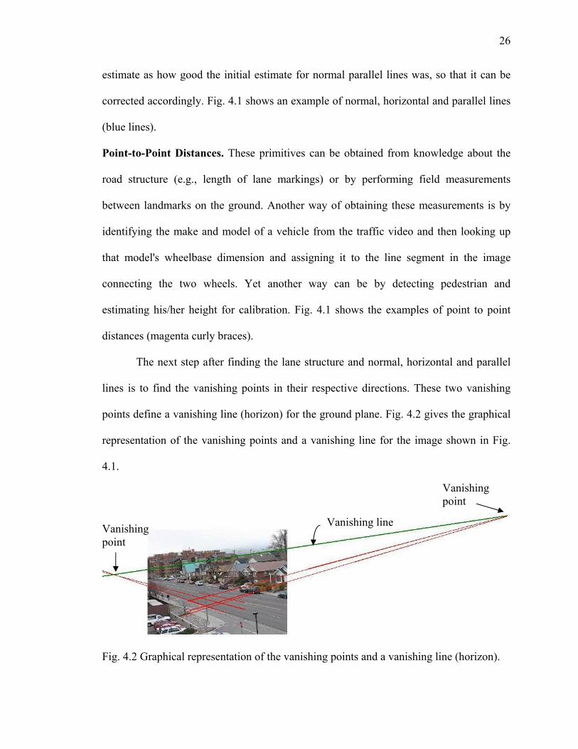
The next step after finding the lane structure and normal, horizontal and parallel
lines is to find the vanishing points in their respective directions. These two vanishing
points define a vanishing line (horizon) for the ground plane. Fig. 4.2 gives the graphical
representation of the vanishing points and a vanishing line for the image shown in Fig.
4.1.
Fig. 4.2 Graphical representation of the vanishing points and a vanishing line (horizon).
Vanishing point
Vanishing line
Vanishing point
27
If only two distinct lines are known, they are enough to estimate the vanishing
point in that direction. However, in general, we have more than two lines for the lane
structure and we can estimate the position of the vanishing point more precisely. If the
two points on a line are p1 = (x1,y1,1) and p2 = (x1’,y1’,1) in homogeneous coordinates,
then the equation of the line is given by a1x+b1y+c1 = 0. Equation of the line can be
written in terms of coefficients (a1,b1,c1) = p1×p2, where × represents cross-product. If we
have multiple parallel lines in the same direction, then the system of equations can be
written as,
⎥⎥⎥⎥⎥⎥
⎦
⎤
⎢⎢⎢⎢⎢⎢
⎣
⎡
−
−−
=⎥⎦
⎤⎢⎣
⎡
⎥⎥⎥⎥⎥⎥
⎦
⎤
⎢⎢⎢⎢⎢⎢
⎣
⎡
nnn c
cc
yx
ba
baba
.
.....
2
1
22
11
. (4.1)
This over-determined system of equations is solved using SVD (Singular Value
Decomposition) to best estimate the coordinates (x,y) of the vanishing point.
If the input primitives include a lane structure and two or more normal lines or
two or more horizontal lines, two vanishing points in orthogonal directions are computed
as above. These points are sufficient to compute four of the five camera parameters. The
remaining parameter (camera height) can then be computed as a scale factor that makes
model distances similar to what they should be. The following describes these steps in
detail. To better understand the position of camera coordinate system with respect to the
world coordinate system, Fig. 4.3 can be referred. The X-Y plane of the world coordinate
system refers to the ground plane coordinate system.

28
Fig. 4.3 World and camera coordinate system.
First, we compute the focal length from the two vanishing points. Without loss of
generality, let vx and vy be the two vanishing image points corresponding to the ground's
X- and Y-axes. Also, based on our assumptions on the camera intrinsic parameters, let
0
0
00 ,0 0 1
uA v
αα
⎡ ⎤⎢ ⎥= ⎢ ⎥⎢ ⎥⎣ ⎦
(4.2)
where, α is the focal length in pixels, and (u0, v0) is the principal point.
In the camera coordinate system, px = A-1[vx 1]T and py = A-1[vy 1]T are the
corresponding vectors through vx and vy respectively (i.e., they are parallel to the
ground's X- and Y-axes, respectively). Since px and py are necessarily orthogonal, their
inner product must be zero:
py . px = 0. (4.3)
ZC
YC XC
Zw
Yw
Xw
h

29
This equation has two solutions for the focal length α. The desired solution is the
negative one and can be written as [50]:
( ).( )x yv D v Dα = − − − − (4.4)
where, D = [u0 v0]T is the principal point. The quantity under the root is the negative of
the inner product of the vectors formed from the principal point to each one of the
vanishing points. Note that in order for the quantity under the root to be positive, the
angle between the two vectors must be greater than 90 degrees. Next, the rotation matrix
can now be formed using normalized px, py, and pz, (the latter computed as the cross
product of the former two) as follows:
[ ]x y zR p p p= . (4.5)
To check the validity of R, the inner product of R and RT can be computed to
make sure that it is I (the identity matrix).
Finally, the scale (i.e., camera height) is determined. Using the point-to-point
distances, we can write an over-determined system of equations to solve for displacement
(height) and the scaling factor.
Therefore, the camera calibration matrix M can be written as follows:
[ 1 2 3 4]M M M M M= , (4.6)
where, M1, M2, M3, M4 are column vectors.
The transformation between ground plane and image plane is a simple
homography H which can defined as,
[ 1 2 4]H M M M= , (4.7)

30
whereas H-1 defines the transformation from image plane to the ground plane. So, if the
image point p = [x,y,1] in homogeneous coordinates is known, then the ground plane
coordinates (3D world coordinates with z=0) can be found by the following equation:
1P H p−= . (4.8)
After determining the camera calibration parameters, it is important to construct a
synthetic camera in OpenGL that can re-project 3D models back onto the image plane.
OpenGL synthetic camera takes four parameters: the 3D world coordinates of the point Q
on the ground plane where the principal axis intersects the ground plane, the aspect ratio
of the image, the field of view of the camera, and the vertical (up) vector YC in world
coordinate system. Fig. 4.4 shows the geometrical representation these parameters.
Fig. 4.4 Geometrical representation of synthetic camera parameters.
fov
YC
ZC
Q
R

31
The X- and Y- coordinates of the point Q can be determined using equation (4.8).
The Z-coordinate of the point Q is –height (-h), as can be seen from Fig. 4.3. The aspect
ratio of the image is given by the ratio (Image width/Image height). The field of view of
the camera is given by,
1 .2cos ( )Q RfovQ R
−= , (4.9)
where coordinates for R are determined in a similar way as Q, and Q.R is the inner
product between Q and R. The vertical (up) vector YC in the world coordinate system is
given by:
(( ) )(( ) )C
R Q QYR Q Q× ×
=× ×
. (4.10)
4.2 Background Modeling and Foreground Object Detection
This is another important aspect of many video surveillance systems. It is very
important that this module detects the relevant details of the scene while excluding
irrelevant clutter. It also needs to be fast for real-time processing of video sequences.
We propose to use an adaptive background model for the entire region of
awareness, and for segmenting the moving objects that appear in foreground. Our
approach involves learning a statistical color model of the background, and process a new
frame using the current distribution in order to segment foreground elements. The
algorithm has three distinguishable stages: learning stage, classification stage and post-
processing stage. Fig. 4.5 shows the pseudo-code of our algorithm.

32
Fig. 4.5 Background modeling and foreground object detection algorithm.
Load ROI template For each frame at time t
1. Learning Stage (Process this stage every C frames) For each pixel (u,v) in ROI template If I(u,v) > TROI
then Process pixel (u,v) in current frame
- Update mean for each channel (Red, Green and Blue)
mean(u,v) = (1-LR)*mean(u,v)+LR*I(u,v) - Calculate variance (σ2) for each channel var(u,v) = (1-LR*LR)*var(u,v)+ (LR*(I(u,v)-mean(u,v)))2 If var(u,v) < min_var then var(u,v) = min_var
2. Classification Stage For each pixel (u,v) in ROI template If I(u,v) > TROI
then Process pixel (u,v) in current frame
- If for each channel I(u,v)-mean(u,v)<T*(var(u,v))0.5 then
FGt(u,v) = 0 %Background else FGt(u,v) = 1 %Foreground else FGt(u,v) = 0 %Background
3. Post-processing Stage For each pixel (u,v) in detected foreground
Look into M×M neighborhood and count number of foreground pixels k. If k<Tneig then FGt(u,v) = 0 %Background Do connected component analysis and create a list of blobs %foreground objects For each blob j If Area(blob(j))<min_Area Assign blob j to background %remove it from %foreground %object list

33
Learning stage. In this stage the background model is estimated using pixel values from
consecutive frames. We use all the channels (red, green, and blue) of a color image to
increase the robustness. We assume that the pixel values tend to have Gaussian
distribution and we try to estimate the mean (m) and variance (σ2) of the distribution
using consecutive frames.
As we use a very simple technique for background modeling, it might not be able
to deal with quasi-stationary backgrounds like trees etc. as well as many other
sophisticated techniques would (e.g. MOG [5, 6]). Therefore we use the inherent
information available to us for the traffic scenes. As we assume a fixed camera position
we can declare the region of interest (ROI) in the scene where vehicles will appear. Fig.
4.6 gives an example of traffic scene and its corresponding ROI template. One more
advantage of using a ROI template is that it reduces the overall area to process for
foreground object detection, hence speeding the algorithm.
(a) (b)
Fig. 4.6 An example of traffic scene and its corresponding ROI template. (a) Traffic scene. (b) ROI template.
To account for the most recent changes in the scene, we use the term learning rate
(LR) which tries to accommodate the scene changes faster into the background model.

34
This kind of strategy can help in dealing with sudden light changes in traffic scenes due
to clouds etc. Also, it removes the requirement of restarting the background model
estimation process after a fixed time period. The learning method proposed here does not
need to store historical data other than background itself, reducing the overall memory
requirements. We also use one more threshold here, namely the minimum variance
(min_var). For pixels whose variance is very small, there is very little fluctuation at that
pixel location so far. However if a sudden change occurs at that location which might not
be significant globally, then that pixel will wrongly be classified as foreground.
Parameter min_var removes this problem. The learning stage is run for a fixed number of
frames initially without doing any foreground detection. Generally a couple hundred
frames are more than enough to capture the background model. Subsequently, the
background model is updated every C (a fixed number) frames. The value of C depends
on the frame rate (frames per second - fps) of the video sequence. We found
experimentally that fps/5 works well without substantial loss of details, when fps is 30.
The speed of the algorithm increases substantially by reducing the number of times the
background model needs the updating. The main advantage of using such a simple
technique is that it is relatively fast.
Classification stage. In this stage we classify the image pixels into foreground and
background pixels based on background model. As discussed earlier, we assume
Gaussian distribution for image pixels. Fig. 4.7 gives an example of a Gaussian
distribution and how a pixel is classified.

35
Fig. 4.7 Pixel classification into foreground and background.
As discussed earlier, classification is done only in the ROI. If a new pixel value is
too far away from the mean pixel value for that pixel location according to the
background model, it is classified as foreground. The value of T can be modified to
reduce the classification errors.
Post-processing stage. The classification stage labels the pixels in foreground and
background classes. In this stage, we try to correct any errors from the classification stage
and create a list of foreground objects by grouping the pixels using connected
components analysis.
First, we remove any isolated pixels from the foreground. We found that doing so
decreases the processing time for the connected component analysis that follows it. After
the connected component analysis, we create a list of blobs (foreground objects). This list
is then processed to remove the blobs with very small area. We found that generally blobs
with area less than 60 pixels don’t prove to be much helpful in subsequent processing for
vehicle detection and classification. Therefore, at the end of this stage we have the list of
foreground objects that might or might not be vehicles.
m-T.σ m+T.σm
Background
Foreground Foreground

36
Fig. 4.8 shows an example of detected foreground.
(a) (b)
Fig. 4.8 An example of detected foreground. (a) Original image. (b) Detected foreground.
4.3 Vehicle Pose Estimation Using Optical Flow
We need to estimate the pose of a vehicle for further processing (i.e., vehicle
detection and classification). We use a pyramidal Lucas and Kanade optical flow
technique [98] as implemented in OpenCV [99]. Details of the implementation can be
found in the OpenCV reference manual [100]. Fig. 4.9 shows the pseudo-code of the
algorithm used for vehicle pose estimation.
Our algorithm has two stages: optical flow estimation and pose estimation. In the
first stage, we calculate the pyramidal Lucas and Kanade optical flow for the detected
foreground regions. We observed that without any loss of accuracy, we can estimate the
optical flow after every Tof frames. This serves two purposes: it increases the speed of the
algorithm as we don’t have to calculate optical flow for every frame and the substantial
relative motion between blobs results in robust optical flow detection. The value of Tof
depends on the frame rate (frames per second - fps) of the video sequence. We found that

37
Tof = fps/10 works well for the video sequences we worked on. If some modification of
Tof is needed, then it can be done on-site to improve the outcome.
Fig. 4.9 Algorithm for vehicle pose estimation using optical flow.
In the next stage, we find the average optical flow vector for every blob. The
optical flow feature vectors corresponding to a blob are averaged to get the optical flow
average vector vavg that represents the orientation of the blob. If no vector corresponding
to a blob is found, the blob is removed from the subsequent processing. Then, the angle α
between the vector vavg and the positive Y-axis (both in 3D world coordinate system) is
calculated. However, the vector vavg is represented in the image plane coordinate system.
For each foreground frame at time t 1. Optical flow estimation stage If mod(t,Tof)=0 then - Pop the first frame f1 from the buffer BF - Grab current frame f2 and save it at top of buffer BF - Find optical flow from f1 to f2 using pyramidal Lucas-Kanade algorithm - Save feature vectors v representing optical flow 2. Pose estimation stage For each blob B in the list For each feature vector v found by optical flow If v Є B then - Add v to blob B’s vector list If size(vector list)=0 then - remove the blob from subsequent processing else
- Find average vector vavg and save it with Blob B’s information - Find angle α of vavg w.r.t. positive Y-axis in 3D world coordinate system - Find 3D world coordinates of the center of Blob B
38
Therefore, we need to convert it to the 3D world coordinate system using homography
(discussed earlier in section 4.1) before finding the angle. This resolves the problem of
finding the orientation of a blob. To tackle the problem of finding the location of a blob
in the 3D world coordinate system, we assume that the center of a blob represents the
center of an actual object and all blobs are on the ground plane. Under these assumptions,
the 3D world coordinates (location) of an object can be calculated using the homography.
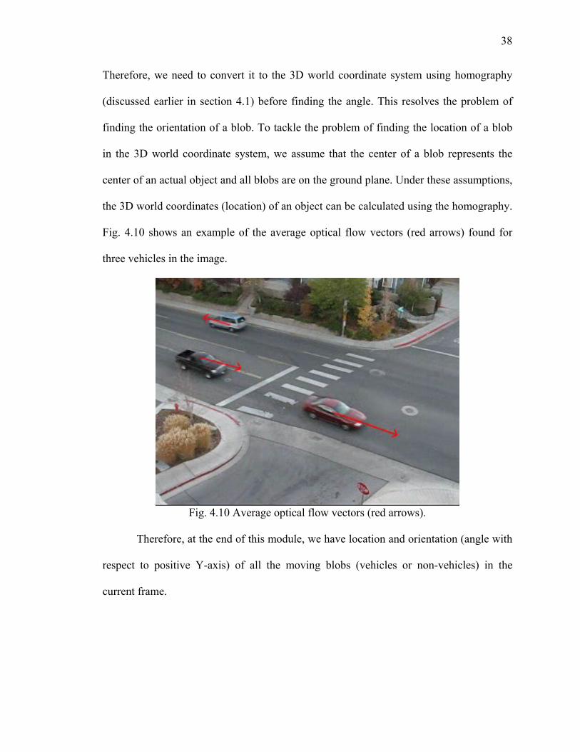
Fig. 4.10 shows an example of the average optical flow vectors (red arrows) found for
three vehicles in the image.
Fig. 4.10 Average optical flow vectors (red arrows).
Therefore, at the end of this module, we have location and orientation (angle with
respect to positive Y-axis) of all the moving blobs (vehicles or non-vehicles) in the
current frame.
39
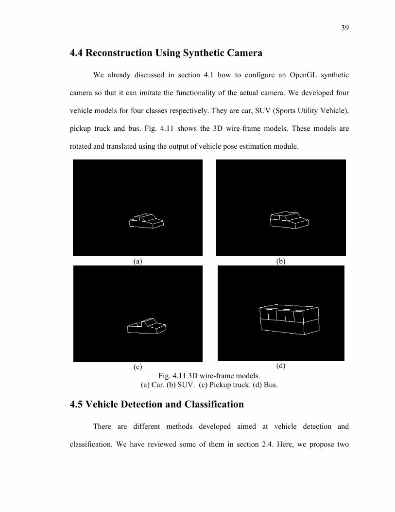
4.4 Reconstruction Using Synthetic Camera
We already discussed in section 4.1 how to configure an OpenGL synthetic
camera so that it can imitate the functionality of the actual camera. We developed four
vehicle models for four classes respectively. They are car, SUV (Sports Utility Vehicle),
pickup truck and bus. Fig. 4.11 shows the 3D wire-frame models. These models are
rotated and translated using the output of vehicle pose estimation module.
(a)
(b)
(c)
(d)
Fig. 4.11 3D wire-frame models. (a) Car. (b) SUV. (c) Pickup truck. (d) Bus.
4.5 Vehicle Detection and Classification
There are different methods developed aimed at vehicle detection and
classification. We have reviewed some of them in section 2.4. Here, we propose two

40
novel methods for vehicle detection and classification. We have incorporated the
detection problem as a part of the classification problem. When the matching score for
any class of vehicle is lower than some threshold then the object is classified as non-
vehicle. The two classification algorithms proposed in this work are a color contour
algorithm and a gradient based contour algorithm.
Before presenting the details of both algorithms, we examine what inputs these
algorithms take. From the foreground object detection module, we have the foreground
frame as shown in Fig. 4.8. Both algorithms try to match object edges with the 3D wire
models. If there are multiple blobs (objects) in an image, we need to segment the blobs
before matching so that only one blob is present in an image. Therefore, if there are n
blobs in an image, we create n separate images with only one blob present in each image.
Then, we use canny edge detector to detect the object edges. Fig. 4.12 shows an example
of such detected edges for a vehicle. This edge template is then matched with the 3D
wire-frame models of the four vehicle classes. However, before doing this matching we
need to rotate and translate the models such that they overlap the actual position of the
vehicle in the image (refer to section 4.4 for more details). After matching is done for all
classes, the best match is assigned as the class of the vehicle under consideration. If the
matching score for all classes is less than some threshold Tmatch, then we classify the
object as non-vehicle. Fig. 4.13 shows the pseudo code algorithm for the vehicle
detection and classification module.
41
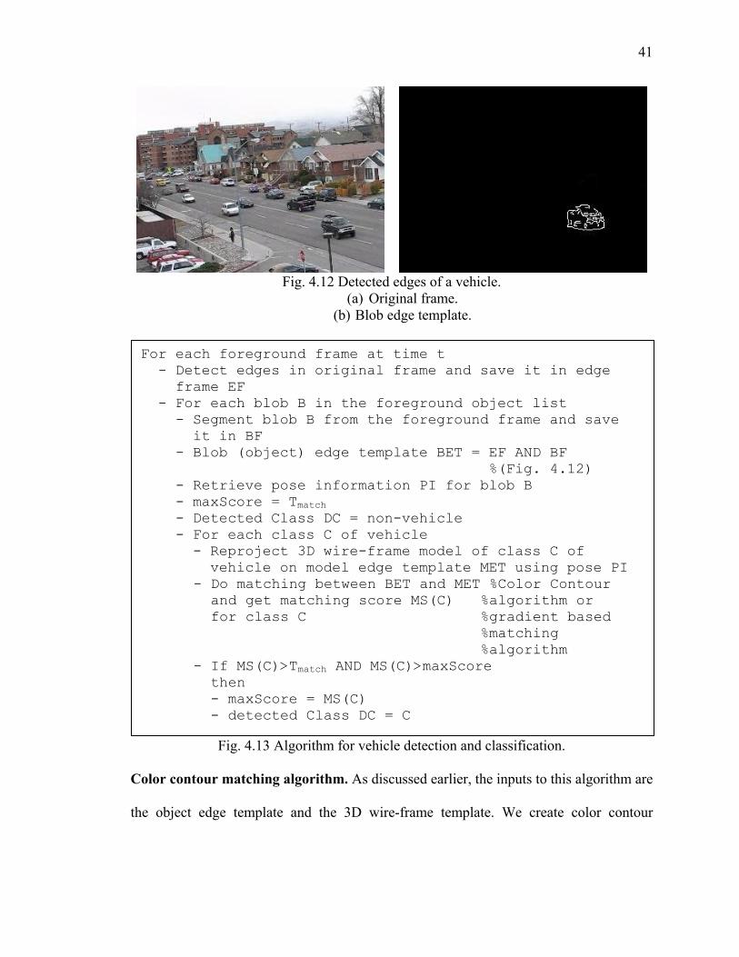
Fig. 4.12 Detected edges of a vehicle.
(a) Original frame. (b) Blob edge template.
Fig. 4.13 Algorithm for vehicle detection and classification.
Color contour matching algorithm. As discussed earlier, the inputs to this algorithm are
the object edge template and the 3D wire-frame template. We create color contour
For each foreground frame at time t - Detect edges in original frame and save it in edge frame EF - For each blob B in the foreground object list - Segment blob B from the foreground frame and save it in BF - Blob (object) edge template BET = EF AND BF %(Fig. 4.12) - Retrieve pose information PI for blob B - maxScore = Tmatch - Detected Class DC = non-vehicle - For each class C of vehicle - Reproject 3D wire-frame model of class C of vehicle on model edge template MET using pose PI
- Do matching between BET and MET %Color Contour and get matching score MS(C) %algorithm or for class C %gradient based %matching %algorithm - If MS(C)>Tmatch AND MS(C)>maxScore then - maxScore = MS(C) - detected Class DC = C
42
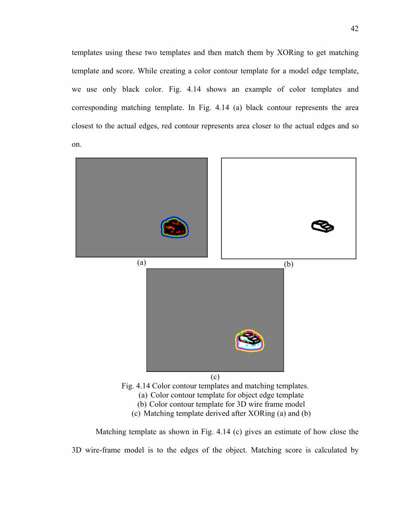
templates using these two templates and then match them by XORing to get matching
template and score. While creating a color contour template for a model edge template,
we use only black color. Fig. 4.14 shows an example of color templates and
corresponding matching template. In Fig. 4.14 (a) black contour represents the area
closest to the actual edges, red contour represents area closer to the actual edges and so
on.
(a)
(b)
(c)
Fig. 4.14 Color contour templates and matching templates. (a) Color contour template for object edge template (b) Color contour template for 3D wire frame model
(c) Matching template derived after XORing (a) and (b)
Matching template as shown in Fig. 4.14 (c) gives an estimate of how close the
3D wire-frame model is to the edges of the object. Matching score is calculated by
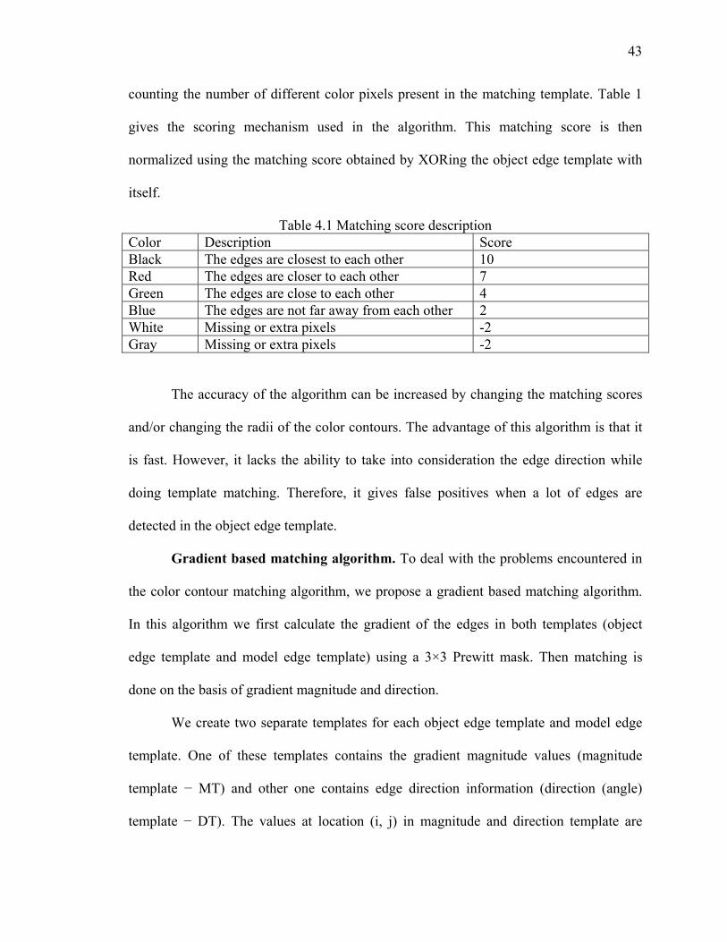
43
counting the number of different color pixels present in the matching template. Table 1
gives the scoring mechanism used in the algorithm. This matching score is then
normalized using the matching score obtained by XORing the object edge template with
itself.
Table 4.1 Matching score description Color Description Score Black The edges are closest to each other 10 Red The edges are closer to each other 7 Green The edges are close to each other 4 Blue The edges are not far away from each other 2 White Missing or extra pixels -2 Gray Missing or extra pixels -2
The accuracy of the algorithm can be increased by changing the matching scores
and/or changing the radii of the color contours. The advantage of this algorithm is that it
is fast. However, it lacks the ability to take into consideration the edge direction while
doing template matching. Therefore, it gives false positives when a lot of edges are
detected in the object edge template.
Gradient based matching algorithm. To deal with the problems encountered in
the color contour matching algorithm, we propose a gradient based matching algorithm.
In this algorithm we first calculate the gradient of the edges in both templates (object
edge template and model edge template) using a 3×3 Prewitt mask. Then matching is
done on the basis of gradient magnitude and direction.
We create two separate templates for each object edge template and model edge
template. One of these templates contains the gradient magnitude values (magnitude
template − MT) and other one contains edge direction information (direction (angle)
template − DT). The values at location (i, j) in magnitude and direction template are

44
calculated using a Gaussian mask of size m×m (i, j) (m=7 is used in our implementation).
Therefore all the edge points in the neighborhood of size m×m (centered at location (i, j))
contribute to the magnitude and direction values depending on their distance from pixel
(i, j). Then, matching template MAT is derived using MT and DT of the blob edge
template (BET) and model edge template (MET) using following equation:
( , ) ( , )* ( , )*cos( ( , ) ( , ))BET MET BET METMAT i j MT i j MT i j DT i j DT i j= − . (4.11)
The matching score is calculated by using matching template MAT using
following equation:
,
,
( , )
( , )i j
selfi j
MAT i jMatchingScore
MAT i j=∑∑
, if ( ) ( )
min( ( ) ( )) match
N BET N METT
N BET N MET−
<−
(4.12)
2( ( ) ( ))( ), min( ( ), ( ))
,
( , )
( , )
N BET N METi j N BET N MET
selfi j
MAT i je
MAT i j
−−
= ×∑∑
, otherwise,
where:
MATself: Matching template obtained by matching BET with itself
N(BET): No. of edge pixels in blob edge template
N(MET): No. of edge pixels in model edge template
Tmatch: Threshold that allows slack in difference between N(BET) & N(MET).
The benefit of using a gradient based matching is that it takes into consideration
the edge direction. As can be seen from equation (4.11), if directions are the same cos(0)
= 1 and if directions are orthogonal cos(90) = 0. While finding the matching score, we
take into consideration the number of edge pixels available in both BET and MET. We do

45
not scale the matching score down if the difference is less than some threshold Tmatch, but
it is scaled exponentially if the difference is more than Tmatch.
4.6 Vehicle Tracking and Traffic Parameter Collection
The purpose of this module is to bring temporal consistency between the results
found by preceding modules. That means it tries to find correspondence between the
results found at different time instances. The purpose of tracking is to determine that
object x found in frame at time t at location (x, y, z) is the same object y found in frame
at time t+1 at location (x’, y’, z’). There are different approaches proposed in literature to
do object tracking (see section 2.5 for more details). In this work we propose a simple
tracking algorithm based on blob tracking. The advantage of this algorithm is that it is
fast. Fig. 4.15 shows the pseudo code of the tracking algorithm.
Fig. 4.15 Algorithm for vehicle tracking
For each frame in the video sequence For each blob (object) B1 at current time t For each blob (object) B2 in track list Find distance d between centers of B1 and B2 in 3D world coordinate system If d < Tdist then If B2 was updated at current time t then Combine B1 and B2 else If B1 and B2 have same pose (angle) then Replace B2 with B1 and update B2’s history information with B1 else Add B1 to track list For each blob (object) B1 in track list If B1 was not updated at current time then Remove B1

46
In terms of traffic parameter collection, we keep record of how each track was
classified in each frame, the no. of active tracks (vehicles) present at any time, velocity of
each vehicle at current time, average velocity of each vehicle during the entire time when
it was visible in the camera’s field of view. The velocity of the vehicle can be found by
using the tracks’ location information. If a vehicle X was observed at location (x, y, z) in
3D world coordinates at time frame t, and if the same vehicle X (belongs to the same
track, assuming tracking was successful) was observed at location (x’, y’, z’) at time
frame t+τ, then instantaneous velocity is given by,
2 2 2( ') ( ') ( ')x x y y z zτ
− + − + − (4.13)
Even though the proposed tracking algorithm is fast and works well when the
traffic scene is not crowded with a lot of vehicles, it fails in case of significant occlusion.
Also, we do not incorporate feature based matching and segmentation of blobs, this might
lead to merging of tracks and detection and classification errors.

47
Chapter 5. Experimental Results
We used our traffic surveillance system to process two video sequences taken
from two different locations. The first video sequence was taken from University of
Nevada parking lot at Virginia Street looking down on Virginia street (VS video
sequence). The second video sequence was taken from University of Nevada parking lot
at N. Sierra Street looking down on Sierra Street (SS video sequence).
The camera calibration process was done offline using Matlab and Mathematica.
The calibration process needs human inputs such as lane structure identification. The
parameters obtained from the camera calibration process were fed to the video
surveillance system that is implemented in C++ using OpenCV.
Fig. 5.1 and Fig. 5.2 show the correctness of camera calibration and pose
estimation routines in VS and SS video sequences respectively.
Fig. 5.1 Models overlapped onto actual vehicles (VS).
(a) Original Frame. (b) After overlapping models onto actual vehicles.

48
(a) (b)
Fig. 5.2 Models overlapped onto actual vehicles (SS). (a) Original Frame. (b) After overlapping models onto actual vehicles.
Fig. 5.3 shows an example of successful tracking. The black SUV that can be seen
in the right part of the image in Fig. 5.3 (a) is track no. 94. This is frame no. 989 of image
sequence VS. The same black SUV can be seen in the center of the image in Fig. 5.3 (b)
with the same track no. 94. This is frame no. 1093 of video sequence VS. The red arrow
shows how the black SUV moved from frame 989 to frame 1093. Therefore, the black
SUV was successfully tracked for more than 100 frames.
(a) (b)
Fig. 5.3 Vehicle tracking (VS). (a) Frame no. 989 of VS. (b) Frame no. 1093 of VS.

49
Fig. 5.4 shows another example of successful tracking in the video sequence SS.
The red car that can be seen in the left part of the image in Fig. 5.4 (a) is track no. 27.
This is frame no. 625 of image sequence SS. The same red car can be seen in the right
hand corner of the image in Fig. 5.4 (b) with the same track no. 27. This is frame no. 675
of video sequence SS. The red arrow shows how the red car moved from frame 625 to
frame 675. This proves that the red car was tracked correctly the entire time it was in the
field of view of camera.
(a) (b)
Fig. 5.4 Vehicle tracking (SS). (a) Frame no. 625 of SS. (b) Frame no. 675 of SS.
Even though the last two results shown for vehicle tracking show that tracking
algorithm works perfectly, there are cases when the tracking fails, especially when there
is occlusion. Fig. 5.5 shows a typical example when the tracking algorithm fails to track a
car when the car occludes a bigger object (a bus). The car had a track no. 22 and the bus
had a track no. 18 (Fig. 5.5 (a)). The car lost its track when it occluded the bus partially.
But, the bus maintained its track (Fig. 5.5 (b)).

50
(a) (b)
Fig. 5.5 Vehicle tracking failure (VS). (a) Frame no. 424 of VS. (b) Frame no. 476 of VS.
Fig. 5.6 shows a snapshot (frame no. 2261) from the VS video sequence. Fig. 5.6
(a) shows the original frame with detected models superimposed. Fig. 5.6 (b) shows the
detected foreground. Fig. 5.6 (c) shows the average optical flow vectors (red arrows). Fig.
5.6 (d) shows the detected edges.
It can be seen from Fig. 5.6 (d) that detecting the class of vehicle on the basis of
edges only is a difficult task. Even human vision would not be able to classify them
correctly if only this edge template was provided to him/her. That explains the quite low
accuracy rates for classification of vehicles.
Table 5.1 and Table 5.2 show quantitative results for the video sequences VS and
SS respectively. The classification results presented here uses gradient based matching.
Vehicle classes are car-(0), SUV-(1), pickup truck-(2), bus-(3) and non-vehicle-(-1). For
the patch of street under surveillance in the VS video sequence, the posted speed limit
was 25 mph, whereas it was 35 mph for the SS video sequence. The average velocity
found by the traffic surveillance system for different vehicles is in accord with the posted

51
speed limits. We do not have ground truth for vehicle velocities to calculate the accuracy
and precision of our method.
(a) (b)
(c) (d)
Fig. 5.6 Traffic surveillance – snapshot (frame no. 2261) from VS. (a) Original frame with detected vehicle class models superimposed.
(b) Detected foreground. (c) Detected optical flow average vectors.
(d) Detected edges of the foreground.
The “Reason for failure” column gives the errors that are not due to classification
methods failure. Classification of vehicles is a daunting task. Most of the errors are due to
lack of or incorrect edge detection. We classify the vehicle based on its classification
results over the entire time when it was on camera’s field of view. We do not take into
consideration the distance of vehicle from camera. Also, no temporal information about

52
the edges detected in the previous frame is saved that might increase the accuracy.
Increasing the details in actual models and increasing the number of classes may improve
the results. However, increasing the number of classes increases the processing time for
classification.
Table 5.1 Quantitative Results for the VS video sequence. Vehicle No.
Track No.
Actual class of vehicle
Maximally detected class of vehicle
Average Velocity (mph)
Reason for failure
1 1 2 2 29.01 2 18 3 3 22.70 3 33 0 0 29.23 4 94 1 0 32.53 5 137 1 or 2 1 22.82 6 195 1 0 27.54
200 1 - 7 200 2 -
Tracking error
8 214 2 0 26.02 9 219 1 0 22.74 10 221 0 0 23.73
241 0 0 11 252 0 0
Tracking error
12 282 1 0 34.95 13 313 0 0 24.73 14 304 0 0 24.95 15 394 0 0 26.96 16 407 0 0 27.88 17 426 1 1 32.17 18 445 1 0 24.71 19 462 1 0 24.40 20 480 2 2 24.86 21 539 1 - Tracking error 22 557 0 0 24.51 23 538 1 or 2 0 24.64 24 572 1 or 2 0 21.52

53
Table 5.2 Quantitative Results for the SS video sequence. Vehicle No.
Track No.
Actual class of vehicle
Maximally detected class of vehicle
Average Velocity (miles/hr)
Reason for failure
1 0 2 2 49.37 2 12 0 0 45.03 3 26 1 2 36.71 4 27 0 2 39.37 5 28 2 2 39.48 6 30 1 2 43.84 7 31 0 0 39.37 8 32 1 0 40.56 9 35 1 -1 Too many edges detected 10 38 0 2 42.05 11 39 2 2 38.54 12 40 2 2 36.70

54
Chapter 6. Conclusions and Future Work
We presented a traffic surveillance system that identifies, classifies and tracks
vehicles. The system is general enough to be capable of detecting, tracking and
classifying vehicles while requiring only minimal scene-specific knowledge.
6.1 Discussion
We used a camera modeling technique that does not require in-lab calibration. A
novel technique was presented that can be used to calibrate the camera on-site. We found
that simple geometric primitives available in the traffic scene could be used to calibrate
the camera parameters efficiently. The overall accuracy of the camera calibration system
was good and it can be verified from the re-projected models that match the actual
position of the vehicles in the image.
The foreground object detection technique used is fast and found to be reliable.
The ROI template technique increases the accuracy dramatically by using prior
knowledge about the scene. Even though this information is needed by the system, it can
be provided on-site by the user.
In this work, we have developed 3D models for 4 classes of vehicles – car, SUV,
pickup truck, and bus. As a part of the project, we developed an API to interface OpenGL
with OpenCV programs.
We also developed vehicle tracking based on simple blob tracking. For the video
sequence VS and SS, the tracking was as high as 90%. It works best when the traffic
scene is less crowded. We were also able to detect the average vehicle speeds using
tracking information recorded by tracking module. The tracking information recorded by

55
the tracking module can be used to find the number of vehicles present in the camera’s
field of view at particular time. It can also be used to find the traffic flow in each
direction. However, partial occlusion and problems due to shadows may lead to tracking
errors.
We found that for the purpose of vehicle detection, the 3D wire-frame models
used in this work are detailed enough that have given high vehicle detection accuracy.
Here, vehicle detection means eliminating possibility of detecting non-vehicles
(pedestrians) as vehicles.
We developed and used two 3D-model based matching techniques, namely color
contour matching and gradient based matching. The results for the first technique are not
given for the reason of a lower classification rate. The second technique also did not
reach expected accuracy (only about 60%). The benefit of using this technique is that it is
fast (5 fps without optimization), compared to the different strategies suggested in the
literature. Also, we did not restrict our view to lateral view with which many researchers
were successful in getting high accuracy. The classification module did not perform as
well as expected. The reason for this is that the data available for classification is
generally noisy. Vehicle classification is the last step after foreground object detection,
vehicle detection, and pose estimation. Therefore, errors in earlier steps slip in vehicle
classification. These reasons can be specifically listed as follows:
• Classification is dependent on tracking such that the class of a vehicle is
determined by successively classifying the vehicle in consecutive frames and then
determining the class based on maximally detected class. Therefore, tracking
errors lead to classification errors.

56
• Poor edge detection may lead to too many or too few edges that might lead to
classification errors.
• Errors in pose estimation lead to classification errors.
• Partial occlusion may lead to classification errors.
Overall, the system works well as far as foreground object detection, tracking,
vehicle detection and vehicle speed estimation are concerned. Because, while choosing
different modules for the system we chose the fastest possible techniques, the system
works at about 5 fps without any optimization. We believe that it can be optimized to
work at real-time speed. The classification of vehicles is still a partially solved problem
that needs further attention.
6.2 Directions of Future Work
Overall, the traffic surveillance system proposed in this work is a step forward in
the right direction. However, more work needs to be done in order to expand the current
system into a full fledged traffic surveillance system. Here we suggest some
improvements that we intend to incorporate in our future work:
• The background modeling and foreground object detection module can be
modified to take into consideration the multimodality of the background. A
technique similar to mixture of Gaussians (MOG) can be used with modifications
to eliminate shadows.
• The vehicle classification technique can be modified to do hierarchical
classification where initial classification is done on the basis of length, width and
area of blob, followed by further classification with detailed 3D class models.
57
This would reduce the number of classes with which the matching process must
be repeated.
• Deformable models can be used that take into consideration various sizes of the
vehicles (e.g., a full size car can be almost as big as a normal sized pickup truck).
• The errors in edge detection lead to classification errors. Some kind of temporal
integrator needs to be used such that edges detected in different frames can be
integrated to best estimate the actual vehicle edges.
• Feature based vehicle tracking can be incorporated in the final system with
occlusion detection.
• Errors in pose estimation need to be corrected and cross-checked with the history
of tracking for that particular vehicle.
• A Kalman filter based vehicle speed estimation system can be included to better
estimate instantaneous vehicle speed.
• Scene-specific information can be used in the final system to detect vehicles
entering a wrong way. If this information is not provided, the system should learn
the normal paths using tracking history of vehicles.
• A stereo camera can be used to retrieve depth information which can be useful in
the vehicle classification process.
• Segmentation can be used to separate partially occluded objects.

58
References [1] E.G.T. Jaspers and J. Groenenboom, “Quantification of the optimal video-coding
complexity for cost-efficient storage,” in Digest of Tech. Papers of the Int. Conf. on Consumer Electronics, Las Vegas, NV, USA, 123–124, Jan. 2005.
[2] Advanced Transportation Management System. [last accessed November 04,
2007]; Available from: http://www.fhwa.dot.gov/environment/cmaqpgs/amaq/03cmaq7.htm.
[3] Intelligent Transportation Systems Research. [last accessed November 04, 2007];
Available from: http://www.tfhrc.gov/its/its.htm. [4] Liyuan Li, Weimin Huang, Irene Y.H. Gu, and Qi Tian, “Foreground Object
Detection from Videos Containing Complex Background,” in Proceedings of the eleventh ACM international conference on Multimedia, Berkeley, CA, USA, 2-10, Nov. 2003.
[5] C. Stauffer and W. Grimson, “Learning patterns of activity using real-time
tracking,” in IEEE Trans. Pattern Analysis and Machine Intelligence, 22:747-757, August 2000.
[6] A. Lipton, H. Fujiyoshi, and R. Patil, “Moving target classification and tracking
from real-time video,” in Proceedings IEEE Workshop on Application of Computer Vision, 8–14, IEEE Computer Society, 1998.
[7] C.Wern, A. Azarbayejani, T. Darrel, and A. Petland, “Pfinder: real-time tracking
of human body,” IEEE Transactions on PAMI, 19(7):780–785, July 1997. [8] T. E. Boult, R. Micheals, X. Gao, P. Lewis, C. Power, W. Yin, and A. Erkan,
“Frame-rate omnidirectional surveillance & tracking of camouflaged and occluded targets,” in Proceedings IEEE Workshop on Visual Surveillance, 48–55, IEEE Computer Society, 1999.
[9] X. Gao, T. Boult, F. Coetzee, and V. Ramesh, “Error analysis of background
adaption,” in Proceedings of IEEE conference Computer Vision and Pattern Recognition, 503–510, IEEE Computer Society, 2000.
[10] I. Haritaoglu, D. Harwood, and L. Davis, “W4: Real-time surveillance of people
and their activities,” in IEEE Trans. Pattern Analysis and Machine Intelligence, 22(8):809–830, August 2000.

59
[11] K. Toyama, J. Krumm, B. Brumitt, and B. Meyers, “Wallflower: Principles and practice of background maintenance,” in Proceedings of IEEE Int’l Conf. on Computer Vision, 255–261, IEEE Computer Society, 1999.
[12] T. E. Boult, R. Micheals, X. Gao, P. Lewis, C. Power, W. Yin, and A. Erkan,
“Frame-rate omnidirectional surveillance & tracking of camouflaged and occluded targets,” in Proceedings IEEE Workshop on Visual Surveillance, 48–55. IEEE Computer Society, 1999.
[13] A. Elgammal, R. Duraiswami, D. Harwood, and L. Davis, “Background and
foreground modeling using nonparametric kernel density estimation for visual surveillance,” in Proceedings of the IEEE, 90:1151–1163, 2002.
[14] A. Mittal and N. Paragios, “Motion-based background subtraction using adaptive
kernel density estimation,” in Proceedings of CVPR, 2:302–309, July 2004. [15] M.K. Leung and Y.H. Yang, “Human body motion segmentation in a complex
scene,” in Pattern Recognition, 20:55–64,1987. [16] C. Ridder, O. Munkelt, and H. Kirchner, "Adaptive background estimation and
foreground detection using Kalmanfiltering," in Proceedings of International Conference on Recent Advances in Mechatronics, 193–199, 1995.
[17] Y. Hsu, H. Nagel, and G. Rekers, “New likelihood test methods for change
detection in image sequences,” Computer Vision Applications, 5:17–34, 1992. [18] Y. Ivanov, A. Bobick, and J. Liu, “Fast lighting independent background
subtraction,” in International Journal of Computer Vision, 37(2):199–207, 2000. [19] G. Gordon, T. Darrell, M. Harville, and J.Woodfill, “Background estimation and
removal based on range and color,” in Proceedings of Computer Vision and Pattern Recognition, 2:459–464, IEEE Computer Society, 1999.
[20] A. Tavakkoli, M. Nicolescu, G. Bebis, "Robust Recursive Learning for
Foreground Region Detection in Videos with Quasi-Stationary Backgrounds,” Proceedings of the International Conference on Pattern Recognition, 315-318, August 2006.
[21] J. P. Tarel, S.S. Ieng, and P. Charbonnier, “Using robust estimation algorithms for
tracking explicit curves,” in Proceedings of European Conference on Computer Vision, 492–507, 2002.
[22] R. P. N. Rao, “Robust Kalman filters for prediction, recognition, and learning,” in
Technical Report 645, University of Rochester, Computer Science, 1996.

60
[23] B. K. Hom, B. G. Schrunck, “Detemining optical flow,” in Artificial Intelligence, 17:185-203, 1981.
[24] A. Bainhridge-Smith, R. G. Lane, “Deremining optical flow using a differential
method,” in Image and Vision Computing, 15:11-22, 1997. [25] L. Wixson, “Detecting salient motion by accumulating directionally-consistent
flow,” in Pattern Analysis and Machine Intelligence, 22(8):774–780, 2000. [26] A. Tavakkoli, M. Nicolescu, G. Bebis, "A Novelty Detection Approach for
Foreground Region Detection in Videos with Quasi-stationary Backgrounds," in Proceedings of the 2nd International Symposium on Visual Computing, Lake Tahoe, Nevada, 40-49, November 2006.
[27] F. Liu and R. Picard, "Finding periodicity in space and time," in Proceedings of
International Conference on Computer Vision, 376–383, 1998. [28] S. Niyogi and E. Adelson, "Analyzing and recognizing walking figures in xyt,”
Proceedings of Computer Vision and Pattern Recognition, 469–474, IEEE Computer Society, 1994.
[29] K. Kim, D. Harwood, and L. S. Davis, “Background updating for visual
surveillance,” in Proceedings of the International Symposium on Visual Computing, 1:337–346, Dec. 2005.
[30] J. Batista, J. Dias, H. Araújo, A. Traça de Almeida, "Monoplanar Camera
Calibration Iterative Multi-Step Approach," in Proceedings of British Machine Vision Conference, 479-488, 1993.
[31] D. C. Brown, "Close-range camera calibration," Photogrammetric Engineering,
37:855-866,1971. [32] W. Faig, "Calibration of close-range photogrammetry systems: Mathematical
foundation," Photogrammetric Engineering in Remote Sensing, 41:1479-1486, 1975.
[33] D. B. Gennery, "Stereo-camera calibration," in Proceedings of Image
Understanding Workshop, 101-108, 1979. [34] Y. I. Abdel-Aziz and H. M. Karar, "Direct Linear transformation into object space
coordinates in close-range photogrammetry," in Proceedings of Symposium on Close-Range Photogrammetry, University of Illinois at Urbana Champaign, Urbana, 1-18, 1971.
61
[35] E. L. Hall,, M. B. K. Tio, C. A. McPherson, and F. A. Sadjadi, "Curved surface measurement and recognition for robot vision," in Conference Records of IEEE workshop on Industrial Applications of Machine Vision, May 1982.
[36] S. Ganapaphy, "Decomposition of Transformation matrices for robot vision," in
Proceedings of International Conference on Robotics and Automation, 130-139, 1984.
[37] T. M. Strat, “Recovering the amera parameters from a transformation matrix,” in
Proceedings of DARPA Image Understanding Workshop, 264-271, Oct. 1984. [38] A. Isaguirre, P. Pu, and J. Summers, "A new development in camera calibration:
calibrating a pair of mobilr cameras," in Proceedings of International Conference on Robotics and Automation, 74-79, 1985.
[39] H. A. Martins, J. R. Birk, and R. B. Kelley, "camera models based on data from
two calibration planes," Computer Graphics Image Processing, 17:173-180, 1981.
[40] M. Fischler and R. Bolles, "Random sample consnsus: A paradigm for model
fitting applications to image analysis and automated cartography," in Proceedings of Image Understanding Workshop, 71-88, 1980.
[41] R. Y. Tsai, “A Versatile Camera Calibration Technique for High-Accuracy 3D
Machine Vision Metrology Using Off-the Shelf TV cameras and Lenses,” in IEEE Journal of Robotics and Automation, RA-3(4):323-343, 1987.
[42] J. Batista, J. Dias, H. Ara'ujo, and A. T. Almeida, "Monoplanar Camera
Calibration - Iterative Multi-Step Approach", in Proceedings of British Machine Vision Conference, 479-488, 1993.
[43] Peter F. Sturm and Stephen J. Maybank, "On Plane-Based Camera Calibration: A
General Algorithm, Singularities, Applications," Proceedings of IEEE conference Computer Vision and Pattern Recognition, 432—437, 1999.
[44] A. Worrall and G. Sullivan and K. Baker, "A simple intuitive camera calibration
tool for natural images," in Proceedings of British Machine Vision Conference, 781-790, 1994.
[45] Ling-Ling Wang and Wen-Hsiang Tsai, "Camera Calibration by Vanishing Lines
for 3D Computer Vision," in Transactions on Pattern Analysis and Machine Vision, 13(4):370-376, 1991.
[46] O. Faugeras, “Three-Dimensional Computer Vision: a Geometric Viewpoint,” MIT
Press, 1993.
62
[47] S. J. Maybank and O. D. Faugeras, “A theory of self-calibration of a moving
camera,” in International Journal of Computer Vision, 8(2):123–152, 1992. [48] R. I. Hartley, “An algorithm for self calibration from several views,” in
Proceedings of the IEEE Conference on Computer Vision and Pattern Recognition, 908–912, June 1994.
[49] Q.-T. Luong and O. Faugeras, “Self-calibration of a moving camera from point
correspondences and fundamental matrices,” in The International Journal of Computer Vision, 22(3):261–289, 1997.
[50] O. Masoud, N. P. Papanikolopoulos, "Using Geometric Primitives to Calibrate
Traffic Scenes," in Proceedings of International Conference on Intelligent Robots and Systems, 2:1878-1883, 2004.
[51] M. Saptharishi, C. S. Oliver, C. P. Diehl, K. S. Bhat, J. M. Dolan, A. Trebi-
Ollennu, and P. K. Khosla, "Distributed surveillance and reconnaissance using multiple autonomous ATVs: CyberScout," in IEEE Transactions on Robotics and Automation, (18):826-836, 2002.
[52] A. Azarbayjani, C. Wren, and A. Pentland, "Real-Time 3D Tracking of the
Human Body," in Proceedings of IMAGE'COM, 1996. [53] A. Bobick, J. Davis, S. Intille, F. Baird, L. Cambell, Y. Irinov, C. Pinhanez, and
A. Wilson., "Kidsroom: Action Recognition in an Interactive Story Environment," in M.I.T.Perceptual Computing, Technical Report 398, 1996.
[54] J. Rehg, M. Loughlin, and K. Waters, ªVision for a Smart Kiosk," in Computer
Vision and Pattern Recognition, 690-696, 1997. [55] T. Olson and F. Brill, “Moving Object Detection and Event Recognition
Algorithms for Smart Cameras,” in Proceedings of DARPA Image Understanding Workshop, 159-175, 1997.
[56] A. Lipton, H. Fujiyoshi, and R. Patil, "Moving Target Detection and
Classification from Real-Time Video," in Proceedings of IEEE Workshop on Application of Computer Vision, 1998.
[57] E. Grimson, C. Stauffer, R. Romano, and L. Lee, "Using Adaptive Tracking to
Classify and Monitoring Activities in a Site," in Proceedings of Computer Vision and Pattern Recognition Conference, 22-29, 1998.

63
[58] E. Grimson and C. Stauffer, "Adaptive Background Mixture Models for Real Time Tracking," in Proceedings of Computer Vision and Pattern Recognition Conference, 1999.
[59] C. Papageorgiou, and T. Poggio, “A Trainable System for Object Detection,” in
International Journal of Computer Vision, 38(1):15-33, 2000. [60] A. Rajagopalan, P. Burlina and R. Chellappa, “Higher Order Statistical Learning
for Vehicle Detection in Images,” in Proceedings of IEEE International Conference on Computer Vision, 2:1204-1209, 1999.
[61] H. Schneiderman and T. Kanade, "A Statistical Method for 3D Object Detection
Applied to Faces and Cars," in Proceedings of International Conference on Computer Vision and Pattern Recognition, 1:746-751, 2000.
[62] P. Burlina, V. Parameswaran and R. Chellappa, “Sensitivity Analysis and
Learning Strategies for Context-Based Vehicle Detection Algorithms,” in Proceedings of DARPA Image Understanding Workshop, 577-584, 1997.
[63] H. Moon, R. Chellappa and A. Rosenfeld, "Performance Analysis of a Simple
Vehicle Detection Algorithm, Image and Vision Computing," 20(1):1-13, 2002. [64] T. Zhao and R. Nevatia, "Car detection in low resolution aerial images," in
Proceedings of International Conference on Image Processing, 710-717, 2001. [65] Z. Chunrui and M.Y. Siyal, "A new segmentation technique for classification of
moving vehicles," in Proceedings of Vehicular Technology Conference, 1:323-326, 2000.
[66] S. Gupte, O. Masoud, R. F. K. Martin, and N. P. Papanikolopoulos, “Detection
and Classification of Vehicles,” in IEEE Transactions on Intelligent Transportation Systems, 3(1):37-47, 2002.
[67] R. P. Avely, Y. Wang, and G. S. Rutherford, "Length-Based Vehicle
Classification Using Images from Uncalibrated Video Cameras," in Proceedings of lntelllgent Transportation Systems Conference, 2004.
[68] C. Zhang, X. Chen, W. Chen, "A PCA-based Vehicle Classification Framework,"
in Proceedings of International Conference on Data Engineering Workshops, 17-17, 2006.
[69] M. W. Koch, K. T. Malone "A Sequential Vehicle Classifier for Infrared Video
using Multinomial Pattern Matching," in Proceedings of the Conference on Computer Vision and Pattern Recognition Workshop, 127-133, 2006.
64
[70] K. M. Simonson, “Multinomial Pattern Matching: A Robust Algorithm for Target Identification,” in Proceedings of Automatic Target Recognizer Working Group, 1997.
[71] C. Huang and W. Liao, "A Vision-Based Vehicle Identification System," in
Proceedings Conference on Pattern Recognition, 4:364-367, 2004. [72] P. Ji, L. Jin, X. Li, "Vision-based Vehicle Type Classification Using Partial Gabor
Filter Bank," in Proceedings of the International Conference on Automation and Logistics, 1037-1040, 2007.
[73] A. Santhanam, M. Rahman, "Moving Vehicle Classification Using Eigenspace,"
in Proceedings of the International Conference on Intelligent Robots and Systems, 3849-3854, 2006.
[74] X. Ma, W. E. L. Grimson, "Edge-based rich representation for vehicle
classification," in Proceedings of the International Conference on Computer Vision, 2:1185-1192, 2006.
[75] R. Wijnhoven, P. H. N. de, "3D Wire-frame Object-Modeling Experiments for
Video Surveillance," in 27th Symposium on Information Theory, 101-108, June 2006.
[76] Brendan Morris and Mohan Trivedi, "Robust Classification and Tracking of
Vehicles in Traffic Video Streams," in Transactions on Intelligent Transportation Systems Conference, 1078-1083, 2006.
[77] J. Hsieh, S. Yu, Y. Chen, and W. Hu, "Automatic Traffic Surveillance System for
Vehicle Tracking and Classification," in Transactions on Intelligent Transportation Systems, 7(2):175-187, 2006.
[78] D. Magee, "Tracking multiple vehicles using foreground, background and motion
models," In Proceedings of ECCV Workshop on Statistical Methods in Video Processing, 2002.
[79] D. Daily, F.W. Cathy, and S. Pumrin, "An algorithm to estimate mean traffic
speed using uncalibrated cameras," In Conference for Intelligent Transportation Systems, 98-107, 2000.
[80] J. Malik and S. Russell, “Traffic Surveillance and Detection Technology
Development: New Traffic Sensor Technology,” California PATH Research Final Report, University of California, Berkeley, UCB-ITS-PRR-97-6, 1997.

65
[81] D. Koller, J. Weber, T. Huang, J. Malik, G. Ogasawara, B. Rao, and S. Russell, “Toward robust automatic traffic scene analysis in real-time,” in Proceedings of International Conference on Pattern Recognition, 126–131, 1994.
[82] D. Koller, K Dandilis, and H. H. Nagel, "Model based object tracking in
monocular image sequences of road traffic scenes," in International Journal of Computer Vision, 10(3):257–281, 1993.
[83] M. Haag and H. Nagel, "Combination of edge element and optical flow estimate
for 3D model-based vehicle tracking in traffic image sequences," in International Journal of Computer Vision, 35(3):295–319, 1999.
[84] J. M. Ferryman, A. D. Worrall, and S. J. Maybank, "Learning enhanced 3d
models for vehicle tracking," in British Machine Vision Conference, 873–882, 1998.
[85] C. Schlosser, J. Reitberger, and S. Hinz, “Automatic car detection in high
resolution urban scenes based on an adaptive 3D-model,” In EEE/ISPRS Joint Workshop on Remote Sensing and Data Fusion over Urban Areas, 98–107, 2003.
[86] T. N. Tan, G. D. Sullivan, and K. D. Baker, “Model-based localization and
recognition of road vehicles,” in International Journal of Computer Vision, 27(1):5–25, 1998.
[87] T. N. Tan and K. D. Baker, “Efficient image gradient based vehicle localization,”
in IEEE Transactions on Image Processing, 9:1343–1356, Aug. 2000. [88] A. E. C. Pece and A. D.Worrall, “Tracking without feature detection,” in
Proceedings of International Workshop on Performance Evaluation of Tracking and Surveillance, 29-37, 2000.
[89] H. Kollnig and H. H. Nagel, “3D pose estimation by directly matching polyhedral
models to gray value gradients,” in International Journal of Computer Vision, 23(3):283–302, 1997.
[90] S. Kamijo, K. Ikeuchi, and M. Sakauchi, "Vehicle tracking in low-angle and front
view images based on spatio-temporal markov random fields," in Proceedings of the 8th World Congress on Intelligent Transportation Systems, 2001.
[91] D. Beymer, P. McLauchlan, B. Coifman, and J. Malik, "A real time computer
vision system for measuring traffic parameters," in Proceedings of Conference on Computer Vision and Pattern Recognition, 495–501, 1997.

66
[92] T. J. Fan, G. Medioni, and G. Nevatia, “Recognizing 3D objects using surface descriptions,” in IEEE Transactions on Pattern Analysis and Machine Intelligence, 11:1140–1157, 1989.
[93] B. Coifman, D. Beymer, P.McLauchlan, and J. Malik, “Areal-time computer
vision system for vehicle tracking and traffic surveillance,” in Transportation Research C, 6(4):271–288, 1998.
[94] N. K. Kanhere, S. T. Birchfield, and W. A. Sarasua, "Vehicle Segmentation and
Tracking in the Presence of Occlusions," in Transportation Research Board Annual Meeting, 2006.
[95] Chachich, A. A. Pau, A. Barber, K. Kennedy, E. Oleiniczak, J. Hackney, Q. Sun,
E. Mireles, "Traffic sensor using a color vision method," in Proceedings of the International Society for Optical Engineering, 2902:156-164, 1997.
[96] Z. Sun, G. Bebis, R. Miller, "Improving the Performance of On-Road Vehicle
Detection by Combining Gabor and Wavelet Features," in Proceedings of the IEEE International Conference on Intelligent Transportation Systems, 2002.
[97] Open Graphics Library. [last accessed November 19, 2007]; Available from:
http://www.opengl.org/. [98] B. D. Lucas, T. Kanade, "An Iterative Image Registration Technique with an
Application to Stereo Vision," in Proceedings of Imaging Understanding Workshop, 121-130, 1981.
[99] Open Computer Vision Library. [last accessed November 20, 2007]; Available
from: http://www.intel.com/technology/computing/opencv/overview.htm. [100] OpenCV Reference Manual.. [last accessed November 20, 2007]; Available from:
http://www.cs.unc.edu/Research/stc/FAQs/OpenCV/OpenCVReferenceManual.pdf.
[101] A. J. Lipton, J. I. Clark, P. Brewe, P. L. Venetianer, and A. J. Chosak,
"ObjectVideo Forensics: Activity-Based Video Indexing and Retrieval for Physical Security Applications," in IEEE Workshop on Intelligent Distributed Surveillance Systems, 56-60, 2004.
[102] D. Duque, H. Santos, P. Cortez, "Prediction of Abnormal Behaviors for Intelligent
Video Surveillance Systems Computational Intelligence and Data Mining," in IEEE Symposium on Computational Intelligence and Data Mining, 362-367, 2007.