Mat

hem

atic

alIn

stit

ute

Uni

vers

ity

ofO

xfor

d

Efficient white noise sampling and coupling for multilevel Monte Carlo

M. Croci (Oxford), M. B. Giles (Oxford), P. E. Farrell (Oxford), M. E. Rognes (Simula)

MCQMC2018 - July 4, 2018

EPSRC Centre for Doctoral Training in Industrially Focused Mathematical Modelling

Mat

hem

atic

alIn

stit

ute

Uni

vers

ity

ofO

xfor

d Overview

Introduction

White noise sampling

Numerical results

Conclusions and further work

Mat

hem

atic

alIn

stit

ute

Uni

vers

ity

ofO

xfor

d Overview

Introduction

White noise sampling

Numerical results

Conclusions and further work

Mat

hem

atic

alIn

stit

ute

Uni

vers

ity

ofO

xfor

d Motivation

The motivation of our research is the sampling of lognormal Gaussian fields. A MaternGaussian field (approximately) satisfies a linear elliptic SPDE of the form

Lu = W , x ∈ D, ω ∈ Ω + BCs,

where u = u(x , ω) and W is spatial white noise. Other approaches can be used (withpros and cons), but we will not discuss them here.

The same techniques can be used to solve a more general class of SPDEs, e.g.

N(u) + Lu = W , x ∈ D, ω ∈ Ω + BCs.

In this case solving means to compute E[P(u)] for some functional P of the solution.

Common applications: finance, geology, meteorology, biology. . .

Main issue: sampling W is hard!

The efficient sampling of W is the focus of this talk.

EPSRC Centre for Doctoral Training in Industrially Focused Mathematical Modelling

Mat

hem

atic

alIn

stit

ute

Uni

vers

ity

ofO

xfor

d Motivation

The motivation of our research is the sampling of lognormal Gaussian fields. A MaternGaussian field (approximately) satisfies a linear elliptic SPDE of the form

Lu = W , x ∈ D, ω ∈ Ω + BCs,

where u = u(x , ω) and W is spatial white noise. Other approaches can be used (withpros and cons), but we will not discuss them here.

The same techniques can be used to solve a more general class of SPDEs, e.g.

N(u) + Lu = W , x ∈ D, ω ∈ Ω + BCs.

In this case solving means to compute E[P(u)] for some functional P of the solution.

Common applications: finance, geology, meteorology, biology. . .

Main issue: sampling W is hard!

The efficient sampling of W is the focus of this talk.

EPSRC Centre for Doctoral Training in Industrially Focused Mathematical Modelling

Mat

hem

atic

alIn

stit

ute

Uni

vers

ity

ofO

xfor

d Motivation

The motivation of our research is the sampling of lognormal Gaussian fields. A MaternGaussian field (approximately) satisfies a linear elliptic SPDE of the form

Lu = W , x ∈ D, ω ∈ Ω + BCs,

where u = u(x , ω) and W is spatial white noise. Other approaches can be used (withpros and cons), but we will not discuss them here.

The same techniques can be used to solve a more general class of SPDEs, e.g.

N(u) + Lu = W , x ∈ D, ω ∈ Ω + BCs.

In this case solving means to compute E[P(u)] for some functional P of the solution.

Common applications: finance, geology, meteorology, biology. . .

Main issue: sampling W is hard!

The efficient sampling of W is the focus of this talk.

EPSRC Centre for Doctoral Training in Industrially Focused Mathematical Modelling

Mat

hem

atic

alIn

stit

ute

Uni

vers

ity

ofO

xfor

d Motivation

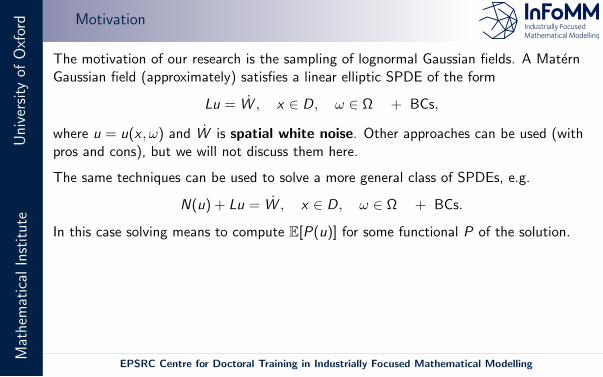
The motivation of our research is the sampling of lognormal Gaussian fields. A MaternGaussian field (approximately) satisfies a linear elliptic SPDE of the form

Lu = W , x ∈ D, ω ∈ Ω + BCs,

where u = u(x , ω) and W is spatial white noise. Other approaches can be used (withpros and cons), but we will not discuss them here.

The same techniques can be used to solve a more general class of SPDEs, e.g.

N(u) + Lu = W , x ∈ D, ω ∈ Ω + BCs.

In this case solving means to compute E[P(u)] for some functional P of the solution.

Common applications: finance, geology, meteorology, biology. . .

Main issue: sampling W is hard!

The efficient sampling of W is the focus of this talk.

EPSRC Centre for Doctoral Training in Industrially Focused Mathematical Modelling

Mat

hem

atic

alIn

stit

ute

Uni

vers

ity

ofO

xfor

d Motivation

The motivation of our research is the sampling of lognormal Gaussian fields. A MaternGaussian field (approximately) satisfies a linear elliptic SPDE of the form

Lu = W , x ∈ D, ω ∈ Ω + BCs,

where u = u(x , ω) and W is spatial white noise. Other approaches can be used (withpros and cons), but we will not discuss them here.

The same techniques can be used to solve a more general class of SPDEs, e.g.

N(u) + Lu = W , x ∈ D, ω ∈ Ω + BCs.

In this case solving means to compute E[P(u)] for some functional P of the solution.

Common applications: finance, geology, meteorology, biology. . .

Main issue: sampling W is hard!

The efficient sampling of W is the focus of this talk.

EPSRC Centre for Doctoral Training in Industrially Focused Mathematical Modelling

Mat

hem

atic

alIn

stit

ute

Uni

vers

ity

ofO

xfor

d White noise (1D)

0 0.1 0.2 0.3 0.4 0.5 0.6 0.7 0.8 0.9 1-150

-100

-50

0

50

100

150

WARNING! Point evaluation not defined!

EPSRC Centre for Doctoral Training in Industrially Focused Mathematical Modelling

Mat

hem

atic

alIn

stit

ute

Uni

vers

ity

ofO

xfor

d White noise (2D)

WARNING! Point evaluation not defined!

IDEA! Avoid point evaluation by integrating W .

EPSRC Centre for Doctoral Training in Industrially Focused Mathematical Modelling

Mat

hem

atic

alIn

stit

ute

Uni

vers

ity

ofO

xfor

d White noise (2D)

WARNING! Point evaluation not defined!

IDEA! Avoid point evaluation by integrating W .

EPSRC Centre for Doctoral Training in Industrially Focused Mathematical Modelling

Mat

hem

atic

alIn

stit

ute

Uni

vers

ity

ofO

xfor

d White Noise (practical definition)

Definition (Spatial White Noise W )

For any φ ∈ L2(D), define 〈W , φ〉 :=∫D Wφ dx . For any φi , φj ∈ L2(D), bi = 〈W , φi 〉,

bj = 〈W , φj〉 are zero-mean Gaussian random variables, with,

E[bibj ] =

∫Dφiφj dx =: Mij , b ∼ N (0,M). (1)

EPSRC Centre for Doctoral Training in Industrially Focused Mathematical Modelling

Mat

hem

atic

alIn

stit

ute

Uni

vers

ity

ofO

xfor

d Finite element (FEM) framework

When solving SPDEs (see 1st slide) with FEM, we get (for linear problems)

Discrete weak form: find uh ∈ Vh s.t. for all vh ∈ Vh,

a(uh, vh) = 〈W , vh〉, (2)

Where Vh = span(φini=0), (e.g. with Lagrange elements).

FEM linear system: uh =∑

i uiφi , u = [u0, . . . , un]T ,

Au = b(ω), (3)

where the entries of b are given by,

〈W , φi 〉(ω) = bi (ω), (4)

with b ∼ N (0,M) as before. M is the mass matrix of Vh.

EPSRC Centre for Doctoral Training in Industrially Focused Mathematical Modelling

Mat

hem

atic

alIn

stit

ute

Uni

vers

ity

ofO

xfor

d Finite element (FEM) framework

When solving SPDEs (see 1st slide) with FEM, we get (for linear problems)

Discrete weak form: find uh ∈ Vh s.t. for all vh ∈ Vh,

a(uh, vh) = 〈W , vh〉, (2)

Where Vh = span(φini=0), (e.g. with Lagrange elements).

FEM linear system: uh =∑

i uiφi , u = [u0, . . . , un]T ,

Au = b(ω), (3)

where the entries of b are given by,

〈W , φi 〉(ω) = bi (ω), (4)

with b ∼ N (0,M) as before. M is the mass matrix of Vh.

EPSRC Centre for Doctoral Training in Industrially Focused Mathematical Modelling

Mat

hem

atic

alIn

stit

ute

Uni

vers

ity

ofO

xfor

d Multilevel Monte Carlo [Giles 2008] + FEM framework

For MLMC, we have two approximation levels ` and `− 1. For any particular ω ∈ Ω, weneed to solve: find u`h ∈ V `

h , u`−1h ∈ V `−1

h s.t. for all v `h ∈ V `h , v `−1

h ∈ V `−1h ,

a(u`h, v`h) = 〈W , v `h〉(ω), (5)

a(u`−1h , v `−1

h ) = 〈W , v `−1h 〉(ω). (6)

This yields the linear system[A` 0

0 A`−1

][u`

u`−1

]=

[b`

b`−1

]= b,

where b ∼ N (0,M). Let V `h = span(φ`i

n`i=0) and V `−1

h = span(φ`−1i n`−1

i=0 ), then

M =

[M` M`,`−1

(M`,`−1)T M`−1

], M`,`−1

ij =

∫φ`iφ

`−1j dx.

NOTE: we do not require the FEM approximation subspaces to be nested!

EPSRC Centre for Doctoral Training in Industrially Focused Mathematical Modelling

Mat

hem

atic

alIn

stit

ute

Uni

vers

ity

ofO

xfor

d Multilevel Monte Carlo [Giles 2008] + FEM framework

For MLMC, we have two approximation levels ` and `− 1. For any particular ω ∈ Ω, weneed to solve: find u`h ∈ V `

h , u`−1h ∈ V `−1

h s.t. for all v `h ∈ V `h , v `−1

h ∈ V `−1h ,

a(u`h, v`h) = 〈W , v `h〉(ω), (5)

a(u`−1h , v `−1

h ) = 〈W , v `−1h 〉(ω). (6)

This yields the linear system[A` 0

0 A`−1

][u`

u`−1

]=

[b`

b`−1

]= b,

where b ∼ N (0,M). Let V `h = span(φ`i

n`i=0) and V `−1

h = span(φ`−1i n`−1

i=0 ), then

M =

[M` M`,`−1

(M`,`−1)T M`−1

], M`,`−1

ij =

∫φ`iφ

`−1j dx.

NOTE: we do not require the FEM approximation subspaces to be nested!

EPSRC Centre for Doctoral Training in Industrially Focused Mathematical Modelling

Mat

hem

atic

alIn

stit

ute

Uni

vers

ity

ofO

xfor

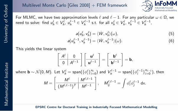
d Multilevel Monte Carlo [Giles 2008] + FEM framework

For MLMC, we have two approximation levels ` and `− 1. For any particular ω ∈ Ω, weneed to solve: find u`h ∈ V `

h , u`−1h ∈ V `−1

h s.t. for all v `h ∈ V `h , v `−1

h ∈ V `−1h ,

a(u`h, v`h) = 〈W , v `h〉(ω), (5)

a(u`−1h , v `−1

h ) = 〈W , v `−1h 〉(ω). (6)

This yields the linear system[A` 0

0 A`−1

][u`

u`−1

]=

[b`

b`−1

]= b,

where b ∼ N (0,M). Let V `h = span(φ`i

n`i=0) and V `−1

h = span(φ`−1i n`−1

i=0 ), then

M =

[M` M`,`−1

(M`,`−1)T M`−1

], M`,`−1

ij =

∫φ`iφ

`−1j dx.

NOTE: we do not require the FEM approximation subspaces to be nested!

EPSRC Centre for Doctoral Training in Industrially Focused Mathematical Modelling

Mat

hem

atic

alIn

stit

ute

Uni

vers

ity

ofO

xfor

d Multilevel Monte Carlo [Giles 2008] + FEM framework

For MLMC, we have two approximation levels ` and `− 1. For any particular ω ∈ Ω, weneed to solve: find u`h ∈ V `

h , u`−1h ∈ V `−1

h s.t. for all v `h ∈ V `h , v `−1

h ∈ V `−1h ,

a(u`h, v`h) = 〈W , v `h〉(ω), (5)

a(u`−1h , v `−1

h ) = 〈W , v `−1h 〉(ω). (6)

This yields the linear system[A` 0

0 A`−1

][u`

u`−1

]=

[b`

b`−1

]= b,

where b ∼ N (0,M). Let V `h = span(φ`i

n`i=0) and V `−1

h = span(φ`−1i n`−1

i=0 ), then

M =

[M` M`,`−1

(M`,`−1)T M`−1

], M`,`−1

ij =

∫φ`iφ

`−1j dx.

NOTE: we do not require the FEM approximation subspaces to be nested!

EPSRC Centre for Doctoral Training in Industrially Focused Mathematical Modelling

Mat

hem

atic

alIn

stit

ute

Uni

vers

ity

ofO

xfor

d Overview

Introduction

White noise sampling

Numerical results

Conclusions and further work

Mat

hem

atic

alIn

stit

ute

Uni

vers

ity

ofO

xfor

d The challenge

SAMPLING PROBLEM 1: single level realisations:sample b ∼ N (0,M), where M is the mass matrix of Vh.

SAMPLING PROBLEM 2: coupled realisations:sample b ∼ N (0,M), where M is the block mass matrix given by V `

h and V `−1h .

EPSRC Centre for Doctoral Training in Industrially Focused Mathematical Modelling

Mat

hem

atic

alIn

stit

ute

Uni

vers

ity

ofO

xfor

d How to sample b?

Sampling b is hard!

Naıve approach

- Factorise M = HHT (cubic complexity!) and set b = Hz, with z ∼ N (0, I ).

⇒ E[bbT ] = E[Hz(Hz)T ] = HE[zzT ]HT = HIHT = M.

- Works well if M diagonal: previous work used either mass-lumping [Lindgren, Rueand Lindstrom 2009], piecewise constant elements [Osborn, Vassilevski and Villa2017] or a piecewise constant approximation of white noise [Drzisga, et al. 2017,Du and Zhang 2002].

- We do not require M to be diagonal (and we do not approximate white noise).

- We can sample b with linear complexity.

IDEA! H does not need to be square, maybe we can find a more efficient factorisation!

EPSRC Centre for Doctoral Training in Industrially Focused Mathematical Modelling

Mat

hem

atic

alIn

stit

ute

Uni

vers

ity

ofO

xfor

d How to sample b?

Sampling b is hard!

Naıve approach

- Factorise M = HHT (cubic complexity!) and set b = Hz, with z ∼ N (0, I ).

⇒ E[bbT ] = E[Hz(Hz)T ] = HE[zzT ]HT = HIHT = M.

- Works well if M diagonal: previous work used either mass-lumping [Lindgren, Rueand Lindstrom 2009], piecewise constant elements [Osborn, Vassilevski and Villa2017] or a piecewise constant approximation of white noise [Drzisga, et al. 2017,Du and Zhang 2002].

- We do not require M to be diagonal (and we do not approximate white noise).

- We can sample b with linear complexity.

IDEA! H does not need to be square, maybe we can find a more efficient factorisation!

EPSRC Centre for Doctoral Training in Industrially Focused Mathematical Modelling

Mat

hem

atic

alIn

stit

ute

Uni

vers

ity

ofO

xfor

d How to sample b?

Sampling b is hard!

Naıve approach

- Factorise M = HHT (cubic complexity!) and set b = Hz, with z ∼ N (0, I ).

⇒ E[bbT ] = E[Hz(Hz)T ] = HE[zzT ]HT = HIHT = M.

- Works well if M diagonal: previous work used either mass-lumping [Lindgren, Rueand Lindstrom 2009], piecewise constant elements [Osborn, Vassilevski and Villa2017] or a piecewise constant approximation of white noise [Drzisga, et al. 2017,Du and Zhang 2002].

- We do not require M to be diagonal (and we do not approximate white noise).

- We can sample b with linear complexity.

IDEA! H does not need to be square, maybe we can find a more efficient factorisation!

EPSRC Centre for Doctoral Training in Industrially Focused Mathematical Modelling

Mat

hem

atic

alIn

stit

ute

Uni

vers

ity

ofO

xfor

d How to sample b?

Sampling b is hard!

Naıve approach

- Factorise M = HHT (cubic complexity!) and set b = Hz, with z ∼ N (0, I ).

⇒ E[bbT ] = E[Hz(Hz)T ] = HE[zzT ]HT = HIHT = M.

- Works well if M diagonal: previous work used either mass-lumping [Lindgren, Rueand Lindstrom 2009], piecewise constant elements [Osborn, Vassilevski and Villa2017] or a piecewise constant approximation of white noise [Drzisga, et al. 2017,Du and Zhang 2002].

- We do not require M to be diagonal (and we do not approximate white noise).

- We can sample b with linear complexity.

IDEA! H does not need to be square, maybe we can find a more efficient factorisation!

EPSRC Centre for Doctoral Training in Industrially Focused Mathematical Modelling

Mat

hem

atic

alIn

stit

ute

Uni

vers

ity

ofO

xfor

d White noise sampling: single level realisations

SAMPLING PROBLEM 1: need to sample b ∼ N (0,M).

Exploit the FEM assembly

M = LT

M1 0 · · ·

0 M2. . .

.... . .

. . .

L = LTdiage(Me)L. (7)

EPSRC Centre for Doctoral Training in Industrially Focused Mathematical Modelling

Mat

hem

atic

alIn

stit

ute

Uni

vers

ity

ofO

xfor

d White noise sampling: single level realisations

SAMPLING PROBLEM 1: need to sample b ∼ N (0,M).

Exploit the FEM assembly

N (0,M) ∼ b = LT

b1

b2...

= LT vstacke(be) (8)

EPSRC Centre for Doctoral Training in Industrially Focused Mathematical Modelling

Mat

hem

atic

alIn

stit

ute

Uni

vers

ity

ofO

xfor

d White noise sampling: single level realisations

SAMPLING PROBLEM 1: need to sample b ∼ N (0,M).

Exploit the FEM assembly

- Each be can be sampled as be = Heze with ze ∼ N (0, I ) and HeHTe = Me .

- b = LT vstacke(be) is N (0,M) since

E[bbT ] = LTE[vstacke(be)vstacke(be)T ]L

= LTdiage(He)diage(HTe )L = LTdiage(Me)L = M.

- If the mapping to the FEM reference element is affine (e.g. Lagrange elements onsimplices) we have that Me/|e| = const on each element and only one localfactorisation is needed.

This approach is trivially parallelisable!

EPSRC Centre for Doctoral Training in Industrially Focused Mathematical Modelling

Mat

hem

atic

alIn

stit

ute

Uni

vers

ity

ofO

xfor

d White noise sampling: coupled realisations

SAMPLING PROBLEM 2: need to sample b ∼ N (0,M), where M is now the blockmixed mass matrix.

Definition (Supermesh, [Farrell 2009])

Let A and B be two (possibly non-nested) meshes. Their supermesh S is one of theircommon refinements. A and B are both nested within S .

EPSRC Centre for Doctoral Training in Industrially Focused Mathematical Modelling

Mat

hem

atic

alIn

stit

ute

Uni

vers

ity

ofO

xfor

d White noise sampling: coupled realisations

SAMPLING PROBLEM 2: need to sample b ∼ N (0,M), where M is now the blockmixed mass matrix.

- Factorise locally, this time on each supermesh element.

- Sample b on S , then interpolate/project the result onto A and B (this step can beperformed locally).

- Since A and B are nested within S , this operation is exact. Note that A and Bneed not be nested.

Previous work on white noise coupling for MLMC used either a nested hierarchy [Drzisgaet al. 2017, Osborn et al. 2017] or an algebraically constructed hierarchy ofagglomerated meshes [Osborn, Vassilevski and Villa 2017].

EPSRC Centre for Doctoral Training in Industrially Focused Mathematical Modelling

Mat

hem

atic

alIn

stit

ute

Uni

vers

ity

ofO

xfor

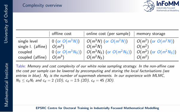
d Complexity overview

offline cost online cost (per sample) memory storage

single level 0 (or O(m3N)) O(m3N) (or O(m2N)) O(m2) (or O(m2N))single l. (affine) O(m3) O(m2N) O(m2)coupled 0 (or O(m3NS)) O(m3NS) (or O(m2NS)) O(m2) (or O(m2NS))coupled (affine) O(m3) O(m2NS) O(m2)

Table: Memory and cost complexity of our white noise sampling strategy. In the non-affine casethe cost per sample can be lowered by precomputing and storing the local factorisations (seeentries in blue). NS is the number of supermesh elements. In our experience with MLMC,NS ≤ cdN` and cd = 2 (1D), cd = 2.5 (2D), cd = 45 (3D).

EPSRC Centre for Doctoral Training in Industrially Focused Mathematical Modelling

Mat

hem

atic

alIn

stit

ute

Uni

vers

ity

ofO

xfor

d Overview

Introduction

White noise sampling

Numerical results

Conclusions and further work

Mat

hem

atic

alIn

stit

ute

Uni

vers

ity

ofO

xfor

d Numerical results: convergence of P(u) = ‖u‖2L2(D)

Consider the linear elliptic SPDE [Lindgren, Rue and Lindstrom 2009], [Bolin, Kirchnerand Kovacs 2017],(

I − κ−2∆)k

u(x , ω) = ηW , x ∈ D ⊆ Rd , ω ∈ Ω, ν = 2k − d/2 > 0.

We compute FEM solutions u`h`=8`=1 with a non-nested hierarchy of subspaces V `

h`=8`=1.

0 1 2 3 4 5 6 7 8

-30

-25

-20

-15

-10

-5

0

5

0 1 2 3 4 5 6 7 8

-70

-60

-50

-40

-30

-20

-10

0

EPSRC Centre for Doctoral Training in Industrially Focused Mathematical Modelling

Mat

hem

atic

alIn

stit

ute

Uni

vers

ity

ofO

xfor

d Numerical results: covariance convergence

C(r) = E[u(x)u(y)] =1

2ν−1Γ(ν)(κr)νKν(κr), r = ‖x − y‖2, κ =

√8ν

λ, x , y ∈ D,

0 0.1 0.2 0.3 0.4

0

0.1

0.2

0.3

0.4

0.5

0.6

0.7

0.8

0.9

1

0 0.1 0.2 0.3 0.4

0

0.1

0.2

0.3

0.4

0.5

0.6

0.7

0.8

0.9

1

0 0.1 0.2 0.3 0.4

0.1

0.2

0.3

0.4

0.5

0.6

0.7

0.8

0.9

1

EPSRC Centre for Doctoral Training in Industrially Focused Mathematical Modelling

Mat

hem

atic

alIn

stit

ute

Uni

vers

ity

ofO

xfor

d Overview

Introduction

White noise sampling

Numerical results

Conclusions and further work

Mat

hem

atic

alIn

stit

ute

Uni

vers

ity

ofO

xfor

d Conclusions and further work

Outlook

- White noise is an extremely non-smooth object and is defined through its integral.

- We can sample single level white noise realisations efficiently.

- We can couple white noise between different FEM approximation subspaces. Asupermesh construction is not needed in the nested case.

- The overall order of complexity is linear in the number of elements of thesupermesh and it can be trivially parallelised. Standard techniques usually havecubic complexity.

Further work: extensions to QMC and MLQMC.

Paper: https://arxiv.org/abs/1803.04857

EPSRC Centre for Doctoral Training in Industrially Focused Mathematical Modelling

Mat

hem

atic

alIn

stit

ute

Uni

vers

ity

ofO

xfor

d References - Thank you for listening!

[1] M. Croci, M. B. Giles, M. E. Rognes, and P. E. Farrell. Efficient white noise sampling and couplingfor multilevel Monte Carlo with non-nested meshes. Preprint, 2018. URLhttps://arxiv.org/abs/1803.04857.

[2] D. Bolin, K. Kirchner, and M. Kovacs. Numerical solutions of fractional elliptic stochastic PDEswith spatial white noise. Preprint, 2017.

[3] D. Drzisga, B. Gmeiner, U. Ude, R. Scheichl, and B. Wohlmuth. Scheduling massively parallelmultigrid for multilevel Monte Carlo methods. SIAM Journal of Scientific Computing, 39(5):873–897, 2017.

[4] Q. Du and T. Zhang. Numerical approximation of some linear stochastic partial differential equationsdriven by special additive noises. SIAM Journal on Numerical Analysis, 40(4):1421–1445, 2002.

[5] M. B. Giles. Multilevel Monte Carlo path simulation. Operations Research, 56(3):607–617, 2008.[6] F. Lindgren, H. Rue, and J. Lindstrom. An explicit link between Gaussian fields and Gaussian

Markov random fields: the stochastic partial differential equation approach. Journal of the RoyalStatistical Society: Series B (Statistical Methodology), 73(4):423–498, 2009.

[7] S. Osborn, P. S. Vassilevski, and U. Villa. A multilevel, hierarchical sampling technique for spatiallycorrelated random fields. Preprint, 2017.

[8] S. Osborn, P. Zulian, T. Benson, U. Villa, R. Krause, and P. S. Vassilevski. Scalable hierarchical PDEsampler for generating spatially correlated random fields using non-matching meshes. Preprint, 2017.

[9] A. J. Wathen. Realistic eigenvalue bounds for the Galerkin mass matrix. IMA Journal of NumericalAnalysis, 7:449–457, 1987.

EPSRC Centre for Doctoral Training in Industrially Focused Mathematical Modelling