University of Central Florida University of Central Florida

STARS STARS

Electronic Theses and Dissertations, 2020-

2020

Efforts in Numerical Modeling of Undulating Propulsion Efforts in Numerical Modeling of Undulating Propulsion

George Loubimov University of Central Florida

Part of the Aerodynamics and Fluid Mechanics Commons

Find similar works at: https://stars.library.ucf.edu/etd2020

University of Central Florida Libraries http://library.ucf.edu

This Masters Thesis (Open Access) is brought to you for free and open access by STARS. It has been accepted for

inclusion in Electronic Theses and Dissertations, 2020- by an authorized administrator of STARS. For more

information, please contact STARS@ucf.edu.

STARS Citation STARS Citation Loubimov, George, "Efforts in Numerical Modeling of Undulating Propulsion" (2020). Electronic Theses and Dissertations, 2020-. 93. https://stars.library.ucf.edu/etd2020/93

EFFORTS IN NUMERICAL MODELING OF UNDULATING PROPULSION

by

GEORGE LOUBIMOVB.S. Aerospace Engineering, The Pennsylvania State University, 2018

A thesis submitted in partial fulfilment of the requirementsfor the degree of Master of Science in Aerospace Engineeringin the Department of Mechanical and Aerospace Engineering

in the College of Engineering and Computer Scienceat the University of Central Florida

Spring Term2020

c© 2020 George Loubimov

ii

ABSTRACT

Naval propulsion is a critical component for every vessel, and it is the subject of this thesis, specif-

ically bio-inspired propulsion. Numerical modeling is used as a tool to understand the relationship

between mechanical undulation and the hydrodynamic response. Through three stages, the re-

search presented here examines and refines tools for understanding fundamentals of undulating

propulsion. Those three objectives are: to verify and validate the proposed numerical models

against existing experiments, establishing a baseline of fidelity; to examine the causal linkage

between fluid-boundary interactions and undulating propulsion; and to create a moment based

method for characterizing generalized undulating propulsive mechanisms. First, a verification and

validation effort is performed for three representative experiments which exhibit key characteris-

tics of undulating propulsion. As a part of these validation efforts, uncertainty quantification is

used to highlight and guide appropriate regions for CFD application. Second, parametric studies

are performed on a simplified undulating bodies to generate an understanding of how localized

mechanical deformations from a generic swimming motion, shape the unsteady fluid dynamics of

the system. Finally, to quantify the performance and efficiency of various swimming motions, a

moment based approach is developed which examines wake profiles and computes efficiency met-

rics. The sum total of these three efforts provides a unified, coherent understanding of common

forms of undulating propulsion and can propel future work in the field.

iii

To my mom, Natasha, and to my uncle, Gennady.

iv

ACKNOWLEDGMENTS

First, I would like to acknowledge the D.O.D. SMART Fellowship for providing funding for my

education and research. I would also like to acknowledge my dear friends Madigan, Jon, Jake,

and Mike for their support and motivation. Finally, I’d like to thank my lab mates Wayne, Renato,

Yigit, and Arinan for their endless help with answering my questions.

v

TABLE OF CONTENTS

LIST OF FIGURES . . . . . . . . . . . . . . . . . . . . . . . . . . . . . . . . . . . . . . ix

LIST OF TABLES . . . . . . . . . . . . . . . . . . . . . . . . . . . . . . . . . . . . . . . xii

CHAPTER 1: INTRODUCTION . . . . . . . . . . . . . . . . . . . . . . . . . . . . . . . 1

CHAPTER 2: LITERATURE REVIEW . . . . . . . . . . . . . . . . . . . . . . . . . . . 6

Modeling . . . . . . . . . . . . . . . . . . . . . . . . . . . . . . . . . . . . . . . . . . 6

Lighthill’s Theory . . . . . . . . . . . . . . . . . . . . . . . . . . . . . . . . . . . 6

Boundary Element Methods . . . . . . . . . . . . . . . . . . . . . . . . . . . . . 8

Computational Fluid Dynamics . . . . . . . . . . . . . . . . . . . . . . . . . . . . 11

Experiments . . . . . . . . . . . . . . . . . . . . . . . . . . . . . . . . . . . . . . . . . 13

Vortex Shedding . . . . . . . . . . . . . . . . . . . . . . . . . . . . . . . . . . . . 13

Thrust Measurement . . . . . . . . . . . . . . . . . . . . . . . . . . . . . . . . . 16

Changes in Kinematic Motion . . . . . . . . . . . . . . . . . . . . . . . . . . . . 17

Burst and Coast Swimming Motions . . . . . . . . . . . . . . . . . . . . . . . . . 18

Validation Experiments . . . . . . . . . . . . . . . . . . . . . . . . . . . . . . . . 19

vi

CHAPTER 3: METHODOLOGY . . . . . . . . . . . . . . . . . . . . . . . . . . . . . . 21

Numerical Modeling . . . . . . . . . . . . . . . . . . . . . . . . . . . . . . . . . . . . 21

Mesh Motion . . . . . . . . . . . . . . . . . . . . . . . . . . . . . . . . . . . . . 21

Heaving and Pitching Motion . . . . . . . . . . . . . . . . . . . . . . . . . . . . . 22

Undulating Motion . . . . . . . . . . . . . . . . . . . . . . . . . . . . . . . . . . 23

Traversing Wing Motion . . . . . . . . . . . . . . . . . . . . . . . . . . . . . . . 24

Uncertainty Quantification . . . . . . . . . . . . . . . . . . . . . . . . . . . . . . . . . 26

Numerical Uncertainty . . . . . . . . . . . . . . . . . . . . . . . . . . . . . . . . 26

Experimental Uncertainty . . . . . . . . . . . . . . . . . . . . . . . . . . . . . . 28

Moment Analysis . . . . . . . . . . . . . . . . . . . . . . . . . . . . . . . . . . . . . . 30

Mean . . . . . . . . . . . . . . . . . . . . . . . . . . . . . . . . . . . . . . . . . 31

Width Factor . . . . . . . . . . . . . . . . . . . . . . . . . . . . . . . . . . . . . 31

Skewness . . . . . . . . . . . . . . . . . . . . . . . . . . . . . . . . . . . . . . . 31

Length Factor . . . . . . . . . . . . . . . . . . . . . . . . . . . . . . . . . . . . . 31

Power Estimation . . . . . . . . . . . . . . . . . . . . . . . . . . . . . . . . . . . 32

Example Moment Study on Stationary Foils . . . . . . . . . . . . . . . . . . . . . 33

CHAPTER 4: FINDINGS . . . . . . . . . . . . . . . . . . . . . . . . . . . . . . . . . . 37

vii

Verification and Validation . . . . . . . . . . . . . . . . . . . . . . . . . . . . . . . . . 37

D-Tube Experiment . . . . . . . . . . . . . . . . . . . . . . . . . . . . . . . . . . 37

Heaving and Pitching NACA 0012 . . . . . . . . . . . . . . . . . . . . . . . . . . 40

Traversing Wing . . . . . . . . . . . . . . . . . . . . . . . . . . . . . . . . . . . . 43

Fluid-Boundary Interactions . . . . . . . . . . . . . . . . . . . . . . . . . . . . . . . . 45

Vortex-Foil Interactions . . . . . . . . . . . . . . . . . . . . . . . . . . . . . . . . 45

Parametric Studies . . . . . . . . . . . . . . . . . . . . . . . . . . . . . . . . . . 48

Moment Analysis . . . . . . . . . . . . . . . . . . . . . . . . . . . . . . . . . . . . . . 55

CHAPTER 5: CONCLUSION . . . . . . . . . . . . . . . . . . . . . . . . . . . . . . . . 60

Verification and Validation . . . . . . . . . . . . . . . . . . . . . . . . . . . . . . . . . 60

Numerical Experiments . . . . . . . . . . . . . . . . . . . . . . . . . . . . . . . . . . . 61

Moment Analysis . . . . . . . . . . . . . . . . . . . . . . . . . . . . . . . . . . . . . . 61

Future Work . . . . . . . . . . . . . . . . . . . . . . . . . . . . . . . . . . . . . . . . . 62

LIST OF REFERENCES . . . . . . . . . . . . . . . . . . . . . . . . . . . . . . . . . . . 64

viii

LIST OF FIGURES

2.1 Illustration of Modeling Methods for Design . . . . . . . . . . . . . . . . . . 11

2.2 von Kármán Vortex Street Behind Cylinder ([6]) . . . . . . . . . . . . . . . . 14

2.3 Reverse von Kármán Wake ([3]) . . . . . . . . . . . . . . . . . . . . . . . . 15

2.4 Experimental Apparatus for Heaving-Pitching Foil ([24]) . . . . . . . . . . . 17

3.1 Heaving-Pitching Experimental Values . . . . . . . . . . . . . . . . . . . . . 23

3.2 Example Heaving-Pitching Foil using Overset Mesh . . . . . . . . . . . . . . 24

3.3 Traveling Wave Model . . . . . . . . . . . . . . . . . . . . . . . . . . . . . 25

3.4 Traversing Wing Mesh . . . . . . . . . . . . . . . . . . . . . . . . . . . . . 26

3.5 Example Mesh Refinement Study . . . . . . . . . . . . . . . . . . . . . . . . 27

3.6 Velocity Profile in Wake . . . . . . . . . . . . . . . . . . . . . . . . . . . . 34

3.7 Velocity Distribution for two Static NACA 0012 Foils . . . . . . . . . . . . . 34

3.8 Moments for Momentum . . . . . . . . . . . . . . . . . . . . . . . . . . . . 35

3.9 Velocity Distribution for two Static NACA 0012 Foils . . . . . . . . . . . . . 35

3.10 Velocity Distribution for two Static NACA 0012 Foils . . . . . . . . . . . . . 36

4.1 Computational Domain and Error Convergence . . . . . . . . . . . . . . . . 38

ix

4.2 Comparison of Experimental and Numerical Shedding Frequency . . . . . . 38

4.3 Comparison of Experimental and Numerical Strouhal Number . . . . . . . . 39

4.4 Periodic Wake Behind D-tube . . . . . . . . . . . . . . . . . . . . . . . . . . 39

4.5 D-Tube Input Uncertainty . . . . . . . . . . . . . . . . . . . . . . . . . . . . 40

4.6 D-Tube Uncertainties . . . . . . . . . . . . . . . . . . . . . . . . . . . . . . 40

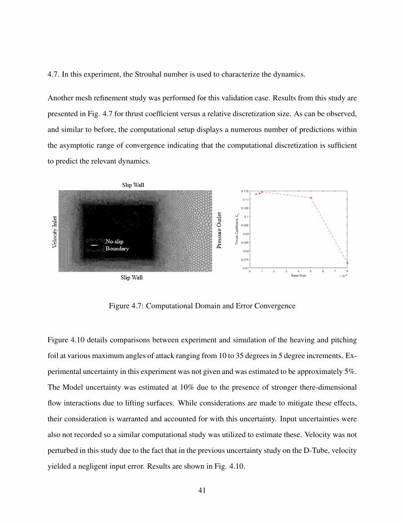
4.7 Computational Domain and Error Convergence . . . . . . . . . . . . . . . . 41

4.8 Heaving-Pitching Foil Input Uncertainty . . . . . . . . . . . . . . . . . . . . 42

4.9 Heaving-Pitching Foil Uncertainties . . . . . . . . . . . . . . . . . . . . . . 42

4.10 Comparison Between Experimental and Numerical Thrust Coefficient . . . . 42

4.11 Wake Resembling von Kármán Vortex Street . . . . . . . . . . . . . . . . . 43

4.12 Traversing Wing Numerical Domain . . . . . . . . . . . . . . . . . . . . . . 44

4.13 Traversing Wing Mesh Refinement Study . . . . . . . . . . . . . . . . . . . 44

4.14 Traversing Wing Uncertainties . . . . . . . . . . . . . . . . . . . . . . . . . 45

4.15 Comparison of Time-Varying Lift . . . . . . . . . . . . . . . . . . . . . . . 45

4.16 Comparison of Time-Varying Drag . . . . . . . . . . . . . . . . . . . . . . . 46

4.17 Foil Separation Schematic . . . . . . . . . . . . . . . . . . . . . . . . . . . 47

4.18 Thrust Coefficient vs Foil Separation . . . . . . . . . . . . . . . . . . . . . . 47

x

4.19 Constructive and Destructive Vortex Interaction . . . . . . . . . . . . . . . . 48

4.20 Parametric Study Variables . . . . . . . . . . . . . . . . . . . . . . . . . . . 49

4.21 Tandem Foil, Secondary Motion Study . . . . . . . . . . . . . . . . . . . . . 50

4.22 Tandem Foil, Concurrent Motion Study . . . . . . . . . . . . . . . . . . . . 51

4.23 Tandem Foil, Secondary Vortex Interaction . . . . . . . . . . . . . . . . . . . 52

4.24 Schooling Configuration, Secondary Foil Motion Study . . . . . . . . . . . . 53

4.25 Schooling Configuration, Positive Vortex Interaction . . . . . . . . . . . . . 54

4.26 Schooling Configuration, Negative Vortex Interaction . . . . . . . . . . . . . 55

4.27 Schooling Configuration, Concurrent Foil Motion Study . . . . . . . . . . . . 56

4.28 Time-Averaged Wake Profiles for Undulating Cases . . . . . . . . . . . . . . 57

4.29 Velocity Distribution in Wake . . . . . . . . . . . . . . . . . . . . . . . . . . 57

4.30 Momentum Moments . . . . . . . . . . . . . . . . . . . . . . . . . . . . . . 58

4.31 Kinetic Energy Moments . . . . . . . . . . . . . . . . . . . . . . . . . . . . 58

4.32 Power Moments . . . . . . . . . . . . . . . . . . . . . . . . . . . . . . . . . 59

xi

LIST OF TABLES

xii

CHAPTER 1: INTRODUCTION

Scientists and engineers throughout history have sought inspiration for new technologies in nature.

Through the process of evolution, biological organisms adapt and evolve to survive in environments

lacking appropriate resources. This leads to the development of highly efficient organisms. Some

examples of this include gecko feet and owl wings. Geckos and other reptilian species have been

studied for their extreme climbing ability. Researchers have been able to develop new adhesion

methods [12, 22] by studying these species. Owls have been known to produce relatively lower

acoustic profiles compared to the ordinary birds – a characteristic attributed to perforations found

in Owl feathers. Researchers have been working on incorporating this to reduce acoustic profiles

of aircraft [10, 23].

In the field of undulation, scientists have observed larger propulsive efficiencies (relative to conven-

tional propeller propulsion) in marine life. One observation noted was the capability of undulating

propulsion to interact with unsteady flow [37, 15, 27]. Due to the unsteady nature of their kine-

matics, marine life is able to morph their external surfaces to operate in an efficient manner as

compared to multi-blade rotors designed for steady state operation without the presence of un-

steady flow. However, marine life is inherently unsteady and operational efficiency in this regime

can be improved if considerations to unsteady flow behaviors are implemented. Thus, it is of in-

terest to understand how propulsive efficiency can be increased while operating in such unsteady

flows. Methods to explore this include experimentation, and numerical simulation. Due to large

complexities associated with flow mixing and visualization, experimental efforts would require

too much time for design work. This leaves numerical simulation as the tool of interest which is

capable of revolving the fluid scales associated with this study.

Therefore, we try to determine how well Computational Fluid Dynamics (CFD) modeling can pre-

1

dict fluid physics associated with undulating propulsion. In this context, high-fidelity numerical

simulations correspond to numerical resolutions that can capture the appropriate fluid dynamics

scales. To answer this question, a detailed verification and validation study with respect to exper-

iments is to be conducted to evaluate the capability of our numerical simulations. This includes

quantifying numerical and experimental uncertainty in the context of numerical mesh resolution

and experimental methods. The output of this study yields important information on the bounds of

our CFD modeling capabilities along with corresponding computational time and determines how

CFD fits in the context of undulating propulsion design.

Three experiments are recreated in CFD, the first being a D-tube shaped obstruction in a flow field

which results in vortex shedding in the form of a von Kármán vortex wake [15]. This experiment

was chosen due to the fact that during particle imagery velocimetry (PIV) studies of undulating

propulsion, a reverse von Kármán vortex wake can be seen. Due to the fact that a stationary D-tube

can create a von Kármán vortex wake, recreating these physics in CFD will show the ability to

predict this physical aspect of undulating propulsion. The second experiment recreated in CFD is

a heaving and pitching NACA 0012 foil generating propulsion [24]. Work done by [4] has shown

that this form of motion can generate propulsion using similar fluid mechanisms associated with an

undulating body. Therefore, validation of this experiment along with the D-tube experiment shows

that the CFD tool-set is capable of recreating the physics associated with undulating propulsion.

The two aforementioned experiments made considerable efforts to mitigate 3D effects. In order

to validate a three-dimensional CFD model, experimental work done in [1] is recreated. Their

experiment involves a linearly traversing rectangular plate which is abruptly heaved and pitched.

The initial angle of attack during the linear traverse is zero before it is linearly increased with a

pitching maneuver. During the pitching maneuver, the plate is also heaved, resulting in an increased

relative angle of attack. The goal of validating this experiment is to draw parallels to the ’burst and

coast’ of swimming - a method composed of impulsive motions and impulsive vortex shedding.

2

These includes vortex shedding from the leading edge and wing tip as well as unsteady loads;

attributes that undulating propulsion would share in a three-dimensional simulation.

The second objective of this study is to improve the understanding of propulsive efficiency in con-

text of tandem swimming. Tandem swimming is defined as any kind of group swimming whether

it be two fish swimming in-line with each other, or a school of fish swimming in arbitrary loca-

tions relative to each other. In evaluating the wakes produced in undulating propulsion, thrust and

drag are mixed, and as such, decomposing the two presents a challenge. This creates complexities

when evaluating results. Using the validated CFD model, we analyze complex boundary-wake

interactions through the use of simplified kinematics.

Due to the low Reynolds number regime and oscillatory nature of undulating propulsion, undula-

tory swimming commonly creates wakes that resemble reverse von Kármán vortex streets [21, 15],

and allows secondary swimmers to interact with these periodic wakes. To explore this, a simpli-

fied model in the form of a heaving and pitching foil is used to create a clear reverse von Kármán

vortex wake. The thrust coefficients of two, tandem, heaving and pitching foils are measured at

various separation distances to quantify the wake-boundary interaction. Due to the clear reverse

von Kármán wake of a heaving and pitching foil, this kinematic approach clearly highlights the

ability of shed vorticies to interact with local surfaces in terms of shearing interactions.

Another numerical case evaluated tandem swimming undulations in a schooling scenario. A lower

order representation of undulating swimmers is utilized in the form of slender bodies. In this

scenario, the previous tandem undulating foil model is modified to include periodic boundary con-

ditions on the inlet, outlet, and walls to simulate a schooling scenario and a pressure gradient is

used to drive the flow. The geometry is simplified to focus on the affects of undulatory motion

such as frequency and amplitude. Parametric studies are conducted on the motions and pressure

gradients to identify which forms of motion prove to be most efficient in a schooling scenario. In

3

these parametric studies, variables are systematically changed to create array matrices of perfor-

mance metrics which are then studied to refine the overall understanding of the interactions. These

studies are applied to the tandem undulating foils in a stand-alone and schooling scenario.

The third and final study centers on methods to interpret simulation data. Specifically, a moment-

based analysis is conducted where time-averaged scalar profiles are examined. These statistical-

like moments can provide information on the distribution of a specific data set. Research done

by [32] explored the characterization of laminar boundary layers by integrating velocity profiles.

Using this approach, one can numerically quantify boundary layer behavior. In this study, the

moments or shape factors are evaluated using the time-averaged velocity within in the wake of

the undulating body. This time-averaged scalar value is then used to ascertain momentum, kinetic

energy, and power distributions across the wake. Moments are then evaluated by integrating these

time averages across the domain. The specific moments we study are defined as mean, width factor,

skewness, and length factor. This approach is used to compare the propulsive efficiencies of two

swimmer geometries with varied motion schemes via the data contained in their wake. Thus, the

use of this method results in more factors to analyze when examining undulating propulsion.

These values give us a description of each quantities’ behavior. Using this approach, we study the

wakes of two undulating swimmers who generate the same time-averaged thrust, but do so using

different motions. We compare the swimming-efficiency of both swimmers by comparing their

respective shape factors. We validate this analysis by solving for each swimming-motion’s required

mechanical power. This secondary validation, allows us to establish a performance baseline from

which we can build our shape factor analysis on. The goal of this study is to predict propulsive

performance using a wake based analysis. We first explore this approach in the context of two

static NACA airfoils to understand shape factor relations. The first foil is a NACA 0012 and the

second is a NACA 0024. In this manner, we can correlate moment relations to known factors of

both foils. With preliminary correlations established, we can then begin to analyze undulating foils

4

and continue the investigation.

The conduction of these three studies should lead to further developments in understanding how

well CFD can be used for predicting undulating performance as well as comprehending where

CFD fits as a design tool. Results from the verification and validation studies will highlight CFD’s

ability to accurately predict the fluid dynamics associated with undulation. The fluid-boundary in-

teraction studies will shed light on CFD’s capability to predict undulating propulsion performance

in external unsteady wakes. The moment based analysis will introduce another method to interpret

simulation results. Future work is also discussed.

5

CHAPTER 2: LITERATURE REVIEW

Modeling

In this section, modeling methods used for predicting forces from undulating propulsion are dis-

cussed. The method discussed include a reactive theory for production (Lighthill’s Theory), un-

steady potential flow methods, and numerical solutions of the Navier Stokes equations. In each

section, the derivation of the theory, including appropriate assumptions and boundary conditions,

will be discussed. Then the theories’ applications and limits will be described.

Lighthill’s Theory

Early methods for predicting forces associated with undulating propulsion can be traced back to

the work done by Lighthill [16]. An outcome of this research was Elongated Body Theory (EBT)

which is based on the assumption that undulating propulsion is derived from reactive forces be-

tween the fluid and local boundary. The three underlying assumptions of this theory include:

• Fluid momentum acts in a perpendicular direction to the local coordinate system of the

swimmer. In a 2D scenario, this would mean that the fluid momentum works perpendicular

to the swimmers spinal chord.

• The mean thrust of the swimmer is estimated using a control volume approach such that the

control volume completely encloses the swimmer.

• During the momentum balance, it is important to estimate and take account of the pressure

forces created by the motion.

6

The use of EBT requires knowledge of the swimmer’s kinematics and corresponding local veloc-

ities where the local reference frame corresponds to the localized surface elements. Again, the

coordinate system used is local to the spinal axis of the swimmer. With knowledge of the kinemat-

ics, the velocity components are estimated as:

u =δxδ t

δxδa

+δyδ t

δyδa

(2.1)

v =δyδ t

δxδa− δx

δ tδyδa

(2.2)

An approximated added mass term is also included:

m =14

πρs2 (2.3)

Where s is the cross sectional area of the swimmer. The momentum, which is a function of con-

vective momentum, pressure forces, and reactive forces, can be now be balanced within the control

volume. The derivation of this vector equation is omitted but the final statement is shown below:

ddt

∫ l

0(− δ z

δa,

δxδa

)daconvective

= [−umv(− δ zδa

,δxδa

)

pressure forces

+12

mv2(δ zδa

,δxδa

)]α=0

reactive forces

− (P,Q) (2.4)

P represents the propulsive force while Q represents the perpendicular forces. A further simplifi-

cation can be made if quasi-steady motions are considered. In this case, the integral term in Eqn.

7

2.4 can be neglected and the mean thrust written as:

Pmean = [mvδyδ t− 1

2v

δxδa

]α=0 (2.5)

While this method can provide preliminary results on momentum based propulsion by use of the

reactive theory, missing elements include considerations to the boundary layer and formulation of

a wake structure. In this case, boundary element methods serve as an excellent step forward as they

enable more complex geometries to be analyzed and make considerations to the boundary layer and

wake structure. The applicability of this theory at this point in time is not warranted as boundary

element methods surpass the accuracy of this theory for similar computational cost. However,

acknowledging this theory is necessary as it was one of the first steps in modeling undulation

based propulsion.

Boundary Element Methods

Boundary element methods (BEM) serve as a precursor to full scale numerical modeling such as

CFD by decoupling the Navier Stokes equations. While each individual BEM may be formulated

differently, the general outline is as follows:

• Utilizing potential flow to solve for the external fluid motion. This includes flow tangency at

the boundary and undisturbed fluid motion at an infinite distance from the boundary.

• Solving the viscous problem via coupling the boundary surface velocity predicted by po-

tential flow to a von Kármán momentum integral analysis in order to estimate the boundary

layer profile.

• Use changes in circulating about the hydrodynamic body to estimate wake shedding structure

8

The potential flow method is applied by defining a velocity potential function

U = ∇Φ (2.6)

where velocity potential satisfies Laplace’s equation

∇2Φ = 0 (2.7)

In essence, the separation of the viscous problem allows one to solve for the fluid behavior as

an elliptic partial differential equation with boundary conditions that enforce flow tangency at the

object boundary and decay of fluid behavior at an infinite space away from the object. Solving for

the external flow field around an object allows for the use of a von Kármán momentum integral

analysis which is based on a differential control volume analysis of the boundary layer. An in depth

derivation is omitted but can be found in [26]. For convenience, the final Momentum integral is:

τwall

ρ= δ

?U∞

dU∞

dx+

ddx

(U2∞θ) (2.8)

where θ can be solved using Thwaite’s method [33]

θ = 0.45ν

u60

∫ x

xstag

u50dx (2.9)

9

Furthermore, a non-dimensional pressure gradient defined as,

λ =θ 2

ν

du0

dx(2.10)

is used to estimate separation where λ = −0.09 is a separation criterion. This value can also be

used to measure the skin friction coefficient using the shear function,

S = (λ +0.09)0.62 (2.11)

where

C f =2ν

u0θ(2.12)

yields the local skin friction coefficient.

Equations 2.8 & 2.9 solve for the laminar boundary layer profiles however they do not account for

turbulent boundary layer behavior. In fact, boundary layer transition criteria can be accounted for

experimentally through the use of shape factors [33]. To account for the wake and correspond-

ing effects on the upstream aerodynamics, a sheet of wake elements is used to capture the fluid

structures. The wake structure is formulated by shedding vorticity elements based on changes in

discrete circulation around the body.

Successful applications of BEM can be seen in [20, 7]. Results show that BEM is a fast compu-

tational tool that can be used for analysis and design of undulating propulsion mechanisms. BEM

serve as an excellent tool for design based on it’s ability to provide fast, accurate performance re-

10

sults for undulating propulsion. Where the use for CFD differs from BEM is it’s ability to capture

fluid-boundary interaction based on developing flow conditions where as BEM seeks to model this

behavior. What this means from a design perspective is that CFD can yield increased refinement in

exchange for large computational time. Where as BEM should be used to narrow down the design

space, CFD can be used to zoom in on specific design specifications to determine more accurate

results.

Figure 2.1: Illustration of Modeling Methods for Design

Computational Fluid Dynamics

With respect to undulating propulsion, CFD simulations are an attractive option as they solve for

the entire flow field, as compared to BEM which solve for the fluid effects on the boundary, CFD

can capture the unsteady fluid interactions at various locations away from the boundary. This is

important for modeling unsteady swimming interaction. For example, consider the example of a

11

swimmer operating in a oscillating vortex street. CFD can capture the advection and diffusion of

these vorticies along with the interaction of a local undulating boundary. Where this differs from

BEM is that this behavior is simulated with the governing equations where as BEM models these

interactions.

Many existing studies [2, 13, 17, 36] have utilized CFD to model the fluid dynamics behind undu-

lating based propulsion. Studies have also been conducted on surface roughness [30] which aims

to examine boundary layer interactions and their effects on downstream thrust production. Other

notable studies include modeling fluid-structure-interactions [28] (FSI) which are aimed at under-

standing how internal marine life skeletal structures interact with the external hydrodynamics.

Due to the low operational Reynolds number range of most marine life swimmer, the use of lam-

inar flow assumptions hold valid and are primarily used to capture fluid-structure interactions. A

scientifically weak area in CFD is that of capturing unsteady fluid transition - due to the laminar

assumptions of modeling undulating propulsion this issue can be avoided. Larger Reynolds num-

ber simulations have also been conducted [5] and make efforts to battle the transition problem. In

the numerical simulations conducted in this work, the Reynolds numbers correspond to laminar

flow conditions.

Common approaches to CFD modeling include comparisons to experimental data as well as numer-

ical uncertainty studies to justify simulation results. The first part of this thesis aims at constructing

a verification and validation study of simulating undulating propulsion with respect to experiments.

This includes appropriate selection of experiments that represent the physics associated with un-

dulating propulsion. Furthermore, experimental and numerical uncertainty are used to create error

bars on the CFD predictions which yield a clearer understanding of the predictions.

12

Experiments

There is an abundance of experimental studies that help provide incremental information on the

physics of undulating propulsion. Most commonly, these experiments are aimed at replicating vi-

sually observed fluid behavior and focusing in on it. The most common observations of undulating

propulsion include:

• Periodic wake composed of counter rotating vortices. This is commonly referred to as a

reverse von Kármán street.

• Changes in swimming gait due to unsteady up-stream wake interactions

• Steady-state vs burst-and-coast forms of motion

In the following sections, experiments targeting these observations and other observations will be

reviewed and discussed. Then, the selection of appropriate experiments for numerical verification

and validation studies will be justified.

Vortex Shedding

A common observed feature in undulating forms of propulsion is the visualization of a reverse

von Kármán vortex street. The formation of an ordinary von Kármán vortex street can be found

around blunt body objects such as cylinders or squares. When these objects are exposes to a

certain cross flow, flow sped outside the wake is significantly higher which causes a shear effect

and consequential vortex formation. An example of a von Kármán vortex street can be visualized

in Fig. 2.2.

13

Figure 2.2: von Kármán Vortex Street Behind Cylinder ([6])

Characterization of a von Kármán vortex street or any shedding vortex formation can be done by

use of the Strouhal number

St =f du

(2.13)

which relates the vortex shedding frequency, object diameter, and cross-flow velocity together into

a non-dimensional parameter. Furthermore, the Strouhal number can be correlated to the Reynolds

number [11] through experiments. This is shown in Eqn. 2.14

St = 0.198(1−19.7/Re) (2.14)

which is valid for Reynolds numbers ranging from 100 to 100,000. Through the use of the relation

in Eqn. 2.14, one can begin to extrapolate the shedding frequency as a function of Reynolds

14

number.

Due to the nature of undulating motion, similar shearing behavior is found between the wake and

external flow of an undulatory swimmer. Furthermore, experiments have visualized the formation

of a reverse von Kármán vortex street. This due to the fact that the wake is moving faster than

the external flow as compared to a static object. This can be seen in Fig. 2.3 which is a particle

imaging velocimetry result of a heaving and pitching foil from experiments conducted in [3].

Experiments in [6] sought to replicate a von Kármán vortex street through the use of circular

cylinders. Similar experiments where done in [15] except with a D-tube shaped geometry. In both

experiments, the shedding frequency was recorded as a function of Strouhal number.

Figure 2.3: Reverse von Kármán Wake ([3])

Ultimately, the wakes observed in Fig. 2.2 and 2.3 represent oscillatory vortexes which are created

by pressure and shearing interactions between two streams of fluid. In the case of a stationary

cylinder, the low pressure zone of the backside of the object is susceptible to instabilities as it

grows which causes the wake from either side if the object to collide. The shearing and pressure

differences between those two wakes cause the shedding vortices to form. A similar case is found

in undulating propulsion; here, the trailing edge undulating object changes it’s circulation and thus

15

sheds a incremental elements of vorticity corresponding to the total change in circulation.

Thrust Measurement

Work done by Betz [4] showed that undulating propulsion could be replicated by a simpler kine-

matic maneuver akin to a heaving and pitching foil. This has allowed for various experiments

[3, 24] to measure thrust as a function of heaving and pitching type motions. A common way to

measure the thrust is as a function of geometric Strouhal number. In this approach, the heaving

amplitude of the heaving maneuver is akin to the diameter of the wake or the von Kármán vortex

street.

In the experiments of [24], an NACA 0012 airfoil was heaved and pitched at certain frequencies

while being linearly traversed in a tow-tank. The equations of motion for the heaving and pitching

are shown below:

y(t) = Ymaxsin( f t). (2.15)

θ(t) = θmaxsin( f t). (2.16)

Figure 2.4 shows the experimental set up from [24].

In the figure, the NACA 0012 wing is ’heaved’ or vertically oscillated while simultaneously

’pitched’ or periodically rotated between the maximum rotational amplitude.

16

Figure 2.4: Experimental Apparatus for Heaving-Pitching Foil ([24])

Changes in Kinematic Motion

Another commonly observed behavior of undulating swimmers is their ability to adjust swimming

kinematics based on unsteady flows. This was hypothesized as not only a means to find a path

of least resistance but also to extract energy from local unsteady structures. In the case of large

periodical vortex structures, it was found that undulating swimmers adjuster their kinematic gait

[15]. Naturally, the unsteady flows found in natural marine habitats is not nearly as structured;

however, the swimmers ability to alter their kinematic gait has ability to reduce energy expenditure

in such unsteady flows.

To further explore this hypothesis, experiments were conducted in [15] which included a rainbow

trout swimming behind a D-tube in a recirculating water tank. Results showed that the presence

of a the D-tube causes the downstream swimmer to alter it’s gait. This alteration did not result in

the swimmer moving further downstream to where unsteadiness would dissipate, nor did it move

to either side of of the wake. In fact, a natural equilibrium was reached where the swimmer moved

17

to a set distance behind the obstruction. To examine where this displacement was purely related to

operating in a low pressure zone such as drafting, various object diameters and flow speeds were

used. These variations changed the periodic flow structure behind the obstruction which followed

the Strouhal number relation shown in Eqn. 2.14. Results showed that for various Strouhal num-

bers and consequential varying vortex structures, the kinematic gait was altered uniquely. Thus the

conclusion was made that swimmers can in fact take advantage of unsteady periodic flows.

Burst and Coast Swimming Motions

Previous studies [34] have shown that some marine swimmers utilize a burst-and-coat form of loco-

motion where an initial impulsive thrust (burst) is generated followed by the swimmer streamlining

its surfaces (coast). These studies have shown that this form of locomotion can be more efficient

compared to steady state locomotion. One caveat to this form of motion is it’s requirement of local

deformations - this causes difficulty in experimentally recreating this form of propulsion. Thus

numerous numerical studies have been conducted [31, 35] to examine this form of locomotion.

One experimental study in [1] sought to model the aerodynamics of bird wings during descent in

a water tank. The geometry included a rectangular wing and tapered wing which are towed and

then heaved and pitched to simulate landing maneuver of a bird wing. While this experiment is

experiment is not directly related to undulating propulsion, the Reynolds range for the experiment

is similar to that of burs and coast swimmers. Furthermore, the applied motions are quite similar -

a gliding motion followed by an impulsive motion which generates excessive force. While results

from this study cannot directly be applied to the study in this thesis, these experiments can be

recreated later on to argue for model validity.

18

Validation Experiments

Based on previous sections, we observe the presence of multiple, discrete fluid phenomena. To

make an argument that our CFD model is capable of recreating all of these physical criteria, we

recreate experiments using CFD. Thus, if we can show that our CFD is capable of recreating

separate physical elements of undulating propulsion, we assume that our CFD model has enough

band-with so to speak to predict coupled fluid interactions.

The key elements that we believe cover our scope are:

• Prediction of periodic wakes

• Measurements of thrust from undulation

• Impulsive thrust generation

By recreating experimental data we can compare and contrast our simulation results, which allows

us to justify our CFD modeling for further, more complex studies. First, we recreate the exper-

iments in [15] which depict the vortex shedding frequency behind a D-tube. While the Strouhal

relation found in Eqn. 2.14 is experimentally compiled for circular cylinders, we chose to model

a D-tube because of its ability to form a periodic wake with lower computational time. This is

because of the abrupt edge of the D-tube on the trailing edge which creates a sharper pressure gra-

dient. Compared to the d-tube, the circular cylinder experiences weaker gradients and thus takes

more computational time for the fluid instability to grow and cause the formation of a periodic

wake.

Secondly, we seek to validate the capability of CFD to replicate thrust measurements from an un-

dulating propulsion mechanism. Experiments in [24], which detail a heaving and pitching foil,

19

are recreated. In these experiments thrust coefficients are measured as a function of heaving and

pitching kinematics. It is important to note that this experiment made significant efforts to mini-

mize three dimensional fluid effects. End plates are utilized to prevent the formation of wing-tip

vortices a characteristic that would come into play for some forms of undulating propulsion. To

account for this, we utilize the experiments in [1] to account for three-dimensional effects as well.

As discussed in the previous section, this experiment involved a linearly towed flat plate that was

impulsively heaved and pitched. Here, strong forms of wing-tip vortex interactions are present.

By recreating these three cases in isolation we can construct the argument that our CFD models are

capable of recreating complex fluid interactions and can be applied to problems involving strong

coupling for two and three dimensional studies. An example of strong coupling in this case would

be a heaving and pitching foil operating in the wake of D-tube or a school of swimmers - cases that

will be examined in further sections. Furthermore, we will study the experimental and numerical

uncertainties associated with these experiments to assess our CFD accuracy.

20

CHAPTER 3: METHODOLOGY

Numerical Modeling

CFD results generated in this effort are based on the commercial CFD code, STAR-CCM+ [29].The

numerical solution method is based on an unsteady, SIMPLE-C segregated solution approach [18].

The model is developed with assumptions of a two-dimensional, laminar, isothermal flow. Under

these assumptions, the mass and momentum equations, expressed in Eqn. 3.1 and 3.2 in indicial

notation, govern the CFD model. The models used in these efforts all have numerical schemes

corresponding to second-order accurate numerics (space and time).

∂ui

∂xi= 0 (3.1)

∂ui

∂ t+

∂uiu j

∂xi=− 1

ρ

∂ p∂xi

+ν∂ 2ui

∂x2i

(3.2)

Within this effort, the fluid properties used represent liquid water. Hence, the bodies operates in a

fluid with ρ = 1000kg/m3 and µlam = 10−3Pa− s. Note that velocity is not always prescribed, but

the general range of velocities is prescribed which for this length scale corresponds to a Reynolds

number range of 1,000 to 50,000 which under oscillatory flow conditions is likely laminar.

Mesh Motion

Foil motion utilizes the Arbitrary Lagrangian Eulerian (ALE) method for foil boundary displace-

ments associated with pitch, heave, and undulation. In this effort, the overset mesh method, Fig.

21

3.2, and mesh morphing, Fig. 3.3, inherit to Star-CCM+ were utilized. Using the overset mesh

scheme, overlapping meshes allow for a solid body displacement to interact with the fluid do-

main.The flow domain is assigned as a background region with it’s own respective mesh while the

moving boundary is the overset region with a different mesh.

In general, overset meshes enable rigid-body motions which does not generally support geometric

deformation associated with undulation. Hence, Mesh deformation is used which enables the

boundary to locally displace with complex functions. This allows for fully undulating motions to

be analyzed. Within the Mesh deformation algorithm of Star-CCM+, the cell vertices are displaced

and redistributed each time step using the BSpline algorithm [29] in the context of the NS-based,

ALE formulation.

We chose to use overset meshes to model the having-pitching airfoil from [24] due to simplification

in simulation development. We then used the mesh deformation to model full body deformation

caused by natural undulation.

Heaving and Pitching Motion

To capture the bulk effects of undulation-based propulsion, a heaving and pitching foil is analyzed

because of available experimental data which can be used in the validation efforts. Work done

by Read [24] details a heaving and pitching NACA 0012 airfoil and records the propulsive forces

generated with respect to Reynolds and Strouhal numbers. Research done by Betz [4] has shown

that this motion can adequately capture the flow physics of undulating propulsion while allowing

for less complex experimentation. This motion model is defined by two combined motions; heave

and pitch. A location along the mid line of the solid body is defined such that the heaving motion of

the foil is centered about this point. With respect to pitch, the rotation of the body is simultaneously

22

Parameter Range Units IncrementSt 0.1 - 0.4 - 0.05

A/C 0.5 - 0.75 - 0.25θmax 10 - 30 degrees 5deg

Figure 3.1: Heaving-Pitching Experimental Values

performed about the same location. The equation for heave motion is specified as

y(t) = Ymaxsin( f t). (3.3)

Here the heave motion has a amplitude of Ymax as well as a driving frequency of f . This pitch

oscillation are driven by the following relationship

θ(t) = θmaxsin( f t). (3.4)

Here, θmax is maximum angle of attack specified, and the pitch oscillation frequency, ω , matches

the heave frequency. A physical description of the motion is presented in the context of an overset

mesh framework in Fig. 3.2. Therein, the heave and pitch dynamics can be observed through

time. In the context of these studies, the parameters are established to replicate experimental

configuration. These parameters are listed in Fig. 3.1.

Undulating Motion

In order to model the undulating foils, the foil is displaced using a travelling wave equation. In

this context, the traveling wave equation intends to model a wave that moves along the foil such

23

Figure 3.2: Example Heaving-Pitching Foil using Overset Mesh

that the undulation push fluid along the the body to create a propelling force. The traveling wave

model used in this work is given by

y(t) = (Ax+b)sin( fxc− vt +φ). (3.5)

This modeled motion is rather complex and requires a detailed explanation. The term given as

Ax+b, represents an amplitude term that is also a function of chord-wise position. Such a feature

is used to enable the study of a wider range of undulation-based motion patterns. The remaining

parameters, f , v, and φ correspond to the spatial frequency (i.e., waves per foil), temporal fre-

quency (i.e., speed of wave), and phase lag, respectively. An example of this motion can be seen

in Fig. 3.3 (for A = 0.2, b = 0.1, and f = 2). Here the chord-dependent amplitude can be observed

along with the adapting computational mesh that captures the complex undulation character.

Traversing Wing Motion

The final experiment used for validation is based on the work completed in [1]. As discussed

previously, the objective of this simulation was to verify the three-dimensional capability of the

24

Figure 3.3: Traveling Wave Model

numerical scheme to predict fluid forces due to unsteady vortex interactions. The Reynolds number

is calculated based on wing chord and tow speed and is approximately 15,000. In this experiment, a

flat plate is first linearly towed in a water tank before being simultaneously heaved and pitched. The

initial angle of attack of the wing section is zero before increasing due to the pitching maneuver.

During the heaving and pitching maneuver, the linear traverse speed is decelerated to a stop. The

prescribed velocities applied to the overset region are shown in Eqn. 3.6, 3.7, and 3.8.

Vx =

Vx,0 t < t1

Vx,0(t2−(t−t1)

t2t1 < t < t2

(3.6)

Vy =

0 t < t0

Vy,0 t1 < t < t2

(3.7)

ω =

0 t < t0

45t2

t1 < t < t2

(3.8)

25

Figure 3.4: Traversing Wing Mesh

Uncertainty Quantification

Numerical Uncertainty

In order to determine the numerical uncertainty associated with the simulated experiments, mesh

refinement studies are evaluated and reported[8, 25, 19]. The objective is to determine an appropri-

ate mesh base size at which the variation of numerical solution is independent with increased mesh

refinement. Figure 3.5 highlights an example of how this study is conducted on a simulation for

lift coefficient estimates on an airfoil. In this figure, lift coefficient is plotted on the y-axis ans the

normalized grid spacing is shown ion the x-axis. Observe the converging region between a normal-

ized grid spacing of 8 and 1; this behaviour corresponds to the numerical solution asymptotically

converging to a constant value.

Furthermore, a Richardson extrapolation can be applied to estimate the infinite grid resolution

value. This is calculated by using previous points in the refinement study within the converging

26

Figure 3.5: Example Mesh Refinement Study

region and the use of Eqn. 3.9

fh=0 =43

f1−13

f2 (3.9)

An order of convergence can also be derived to measure the numerical simulation convergence as

a function of increased mesh refinement. This variable is sued to gauge the quality of asymptotic

convergence regions and shown:

p = ln(f3− f2

f2− f1)/ln(r) (3.10)

where r corresponds to a constant mesh spacing refinement factor.

To estimate for the numerical error contribution, [25] suggested the use of a Grid Convergence

Index (GCI). The GCI is the numerical error between two numerical grids and is calculated using

27

results from a mesh refinement study sing Eqn. 3.11:

GCI =Fs|( f1− f2)/ f1|

rp−1(3.11)

where Fs corresponds to a factor of safety. f1 and f2 correspond to two sequential meshes with

decreasing refinement.

To maintain a highly time-accurate simulation, the Courant–Friedrichs–Lewy (CFL) [14] condition

is utilized by adapting the simulation time-step to maintain a convective Courant number, V dtdx ,

below unity within the entire domain. Hence, as the mesh is refined, the simulation time-step

appropriately reduces to maintain a relatively consistent Courant number.

Experimental Uncertainty

The experimental uncertainty is a combination of uncertainties which stem from replicating a phys-

ical experiment using numerical simulations. It is composed of three core components; experimen-

tal model, and input.

• Experimental: This term is associated with random experimental behaviour. This includes

all non-predictable behaviour which changes the output of the physical experiment. This

includes un-accounted for variables which directly affect the experimental results.

• Model: This term is associated with a lack of information on the experiment and conse-

quential reduction of order in a numerical simulation. For example, surface defects on an

airfoil may cause premature transition in a physical experimental - lack of inclusion of this

geometric feature in numerical simulation could potentially skew the output.

28

• Input: this term is associated with experimental inputs i.e. airspeed in a wind tunnel or geo-

metric angle of attack on an airfoil. It accounts for the uncertainty associated with varying-

accuracy input variables which consequentially skew the output variable.

During the conduction of experiments, these values should all be recorded and presented. In the

case that they are not, the following paragraphs discuss methods of estimating these terms.

In the case that experimental uncertainty is not recorded, this term must be guessed. IN most

cases, this term is lost in the averaging of multiple experimental runs and can range between 1 and

10 percent. This term can be estimated based on complexity of the experiment - in other words

experimental complexity corresponds to the number of interacting variables in the experiment. For

this study, the experimental uncertainty is estimated at five percent for all experiments.

Model uncertainty is another term that must be estimated. Here there are obvious reasons for

model uncertainty such as simplifications from three to two-dimensional simplifications, surface

roughness, and other imperfections in the experimental set up. In this study, this value is estimated

based on an approximate estimate of variation in model geometry.

Input uncertainty can be estimated using a series of perturbation studies. These uncertainties are

approximated by slightly perturbing the numerical input values and examining the changed in

output. Equation 3.12 shows this

u f =δ fδx

ux (3.12)

where u f represents the output uncertainty as a function of ux, the input uncertainty. δ f is cal-

culated by measuring the difference in simulated output based on δx, the perturbation variable x.

In the case where ux is not reported in experimental data, this values must be estimated using the

29

numerical model.

In the previous example, u f represented one input uncertainty. In order to estimate the total input

uncertainty associated with all variables in an experiment, the root mean square is calculate using

Eqn. 3.13.

uinput =√(u f 1)2 +(u f 2)2 +(u f 3)2 + ... (3.13)

Moment Analysis

A novel approach to studying performance of undulating swimmers is now discussed. This ap-

proach involves evaluating moments or shape factors of velocity profiles in the wake of undulating

swimmers. This method serves to compare two forms of swimming kinematics by comparing

wake moments. The shape factors are evaluated through taking integrals of the time-averaged ve-

locity from an arbitrary axial position in the wake. Specifically, the wake is probed to study how

propulsion is generated. Equation 3.14 shows how these moments will be calculated.

Mn =

∫ y−y ρV nykdy∫ y−y ρV n

0 ykdy(3.14)

From Eqn. 3.14, we define k as the statistical moment value and n value as the function of interest

parameter. V is the varying velocity in the wake and V0 is the free-stream velocity. In this study,

we calculate moment coefficients for momentum, kinetic energy, and power within the wake. The

k-values allow us to change the specific statistical moments we are interested in.

30

Mean

By setting the k value to zero, we are able to determine the mean coefficient of a particular function.

The mean moment should yield the average function value across the wake profile. With respect to

two different undulating foils generating the same thrust, the mean momentum should be identical.

Width Factor

The 1st moment, which we call the width factor, is related to the width of the velocity distribution.

In this sense, it determines which profile is wider when comparing two velocity distributions. This

is a valuable quantity because the velocity distributions for a undulating swimmer in self propulsion

are highly correlated to the Strouhal number. The width of the flow has been shown to correlate to

the amplitude of the undulating motion [3]. Therefore, we can use the width factor to learn more

about the specific motion parameters employed by an undulating foil.

Skewness

The skewness will shed light on the unevenness of the distribution. Because we are analyzing

a time-averaged jet flow, we expect this coefficient value to be very close to one. A skewness

moment not equal to unity would show that the jet is not parallel to the intended motion and would

result in a unbalanced propulsive force.

Length Factor

The third moment, or ’Length Factor’, will yield information on the distribution of the profile.

More specifically, this factor can be used to compare the viscous losses between two undulating

31

motions. This will be highlighted in the following section.

Power Estimation

In order to close the study, the power required to generate the swimming motion is evaluated.

The power considered is the mechanical power or the power required to generate the motion and

does not consider power required to move the body in the direction of travel as in the case of

standard power calculations for aircraft. Using these values, we can correlate this information to

the statistical moments calculated within the wake.

The power required is calculated as follows

P = FyVy. (3.15)

Where Fy is the integrated chord wise force perpendicular to the direction of motion. Fy is calcu-

lated from CFD output by integrating the chord-wise pressure and wall shear stress and taking the

component perpendicular to the mean thrust line.

F =∫

cspds+

∫cs

τwallds+∫

csm(dV/dt)ds. (3.16)

In the above equations, we make considerations to forces due to pressure, viscous shearing, and

inertial terms. For the inertial term, we assume the foil is neutrally buoyant and distribute the mass

according to the foil area. Vy represents the integrated chord wise velocity which runs parallel to

the chord wise force. The velocity is solved for by taking the derivative of the motion equation

32

with respect to time.

V = Acos(x− f t) (3.17)

Where

A = (− f )(A1 +A2x+A3x2) (3.18)

Thus, we are able to estimate and compare the power of each motion and establish preliminary

performance metrics. Additionally, the chord wise power can be interrogated to shed more light

on where the energy is expended for propulsion on each foil motion.

Example Moment Study on Stationary Foils

First, consider a study on two NACA airfoils; the NACA 0012 and 0024 (Fig. 3.6). The location of

the integration plane was chosen to be 5 cm back from the trailing edge. This location was chosen

due to the fact that the time-averaged velocity profiles seemed most prominent at this location.

Figure 3.7 is a plot of the velocity distribution in the wake for these airfoils. On the x-axis we have

normalized velocity plotted and on the y-axis we vertical position normalized by chord length. In

Fig. 3.7 it can be observed that the NACA 0024 has a wider and longer velocity distribution due

to flow obstruction. We also know that this foil will experience more drag. With this information

in hand, we can now create correlations with shape factors which are shown in Fig. 3.9, 3.9, and

3.10.

As discussed in the previous section, we make the following correlations regarding the presented

moments. Firstly, we discuss momentum; from Fig. 3.8 we observe that the mean moment is

higher for momentum, kinetic energy, and power of the standard NACA 0012. This is expected as

33

Figure 3.6: Velocity Profile in Wake

Figure 3.7: Velocity Distribution for two Static NACA 0012 Foils

it is known that the double thickness foil will experience more drag. The correlation can now be

made that a lower 0th moment corresponds to lower drag. However, it is not yet apparent what this

drag is composed of (i.e. pressure vs viscous dag).

Moving on to the 1st moment or width factor, we see that the thicker foil now has a higher moment.

As discussed earlier, this moment correlates to the width of the wake. Due to the thicker foils

geometry, we expect the wake to be thicker. Here we draw the second correlation that a higher

1st moment correlates to wake width. Now we will discuss the 2nd moment or skewness. We

34

Figure 3.8: Moments for Momentum

Figure 3.9: Velocity Distribution for two Static NACA 0012 Foils

observe that both values are not equal to unity; however, this behaviour can be explained. Due to

the numerical methods used to calculate the flow-field, we do not expect the velocity distribution to

be perfectly symmetrical. Thus, we can observe that the skewness values do show that the profile

is close to being perfectly symmetrical.

Finally, we examine the 3rd moment or length factor. Here we also see the the thicker foil has a

higher moment for all categories. As discussed before, we attribute this behaviour to length of the

distribution. We know from previous studies that the less-than-unity velocity region in Fig. 3.7

35

Figure 3.10: Velocity Distribution for two Static NACA 0012 Foils

represents momentum losses. We also know that the increase in velocity is representative of flow

acceleration due to area constriction. When examining the flow acceleration of the wider foil, we

see larger velocity values due to more fluid being displaced by the foil. Using all of this informa-

tion, we conclude that the 3rd moment or length factor corresponds to flow acceleration. In the

context of comparing momentum for two cases, this means a larger length factor corresponds to

higher flow acceleration. Furthermore, from visual analysis of Fig. 3.7, we can hypothesize that

the shape factor relates the ratio of losses to gains, where gains represent all velocities above free

stream and losses represent values below free-stream conditions. Using this observation, we con-

clude that this corresponds to higher shearing between the loss and gain regime, which corresponds

to viscous losses. In the following sections we will revisit this study and analyze and compare two

undulating forms of propulsion with various kinematics.

36

CHAPTER 4: FINDINGS

Verification and Validation

D-Tube Experiment

The first benchmark evaluates the ability to capture the vortex shedding created for the flow over

a D-shaped tube represented in previous experiments in a water tunnel [15]. In this experiment,

the Strouhal number is measured based on flow velocity, tube diameter, and vortex shedding fre-

quency. The CFD models the experimental setup using two-dimensional approximations, as the

experiments [15] made significant efforts to mitigate 3D flow effects to create 2D vortex shedding,

the assumption is further justified.

In order to establish the computational mesh and numerical uncertainty, a mesh-independence

study is performed (shown in Fig. 4.1). As discussed in the previous section, this study is con-

ducted by systematic variation of the mesh base size and simulation time-step to maintain an con-

stant Courant number (V ∆t/∆x) with a mean value of approximately unity. Results from this mesh-

independence study are presented in Fig. 4.1. In this plot is the predicted thrust coefficient (y-axis)

versus the representative mesh size (x-axis). To the right of this graph we have the coarser meshes.

The right-most point indicates an erratic solution and that that mesh was non-convergent. How-

ever, moving left of this point a series of 6 subsequently refined results display a clear converging

trend indicating that the mesh/temporal resolution is within the asymptotic range of convergence.

The p value is calculated using Eqn. 3.10 as 1.61 which is reasonably close to the theoretical value

of two. The GCI is shown in Fig. 4.6

The numerical simulation is shown to the left of the mesh refinement study. A velocity inlet and

37

Figure 4.1: Computational Domain and Error Convergence

Figure 4.2: Comparison of Experimental and Numerical Shedding Frequency

pressure outlet are used to drive the flow and a slip-wall boundary condition is used to prevent the

development of a boundary layer. A no-slip boundary condition is applied to the D-tube.

Comparisons of CFD results and experiment are presented in Fig. 4.2. The frequency predicted

predicted by CFD is measured using a fourier transform of the time-varying lift data. This pressure

probe provides a sinusoidal, time varying measurement which allows for extraction of shedding

frequency. In this plot, the measured frequency is shown on the y-axis and is plotted against inlet

38

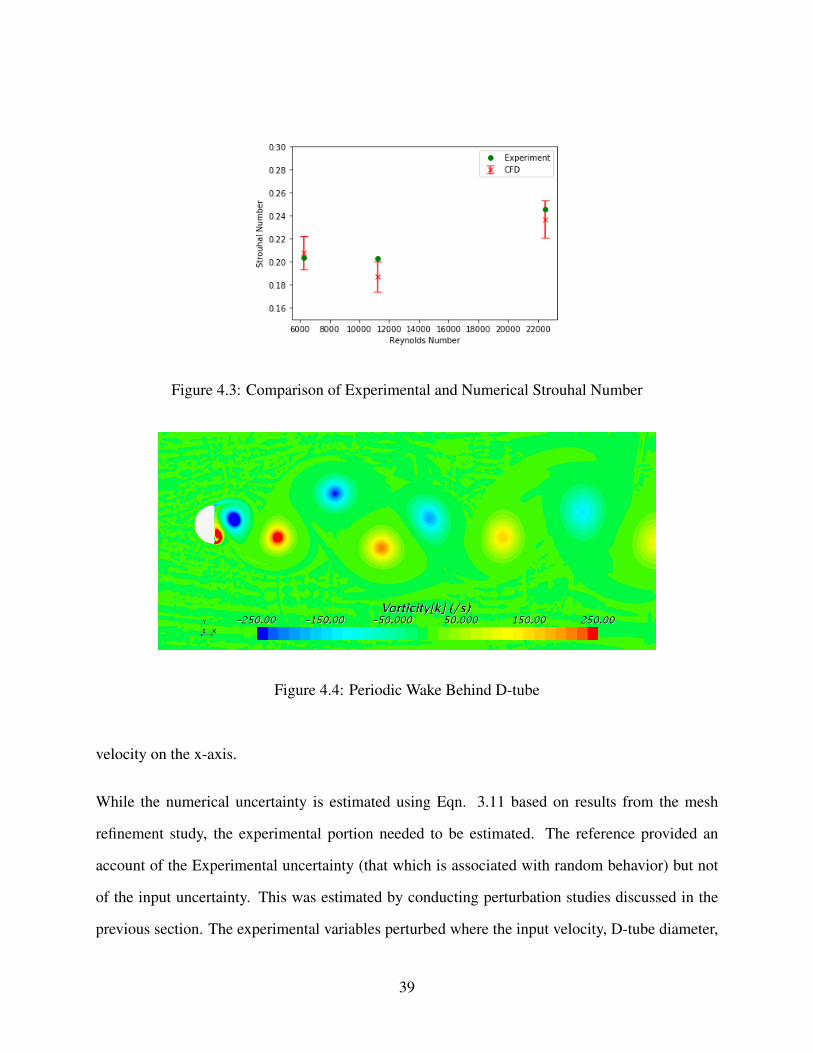
Figure 4.3: Comparison of Experimental and Numerical Strouhal Number

Figure 4.4: Periodic Wake Behind D-tube

velocity on the x-axis.

While the numerical uncertainty is estimated using Eqn. 3.11 based on results from the mesh

refinement study, the experimental portion needed to be estimated. The reference provided an

account of the Experimental uncertainty (that which is associated with random behavior) but not

of the input uncertainty. This was estimated by conducting perturbation studies discussed in the

previous section. The experimental variables perturbed where the input velocity, D-tube diameter,

39

Original Value Perturbed Value d f/dx Input UncertaintiesDiameter 2.5 cm 2.6 cm 0.5 2.5 %Velocity 2.5 m/s 2.6 m/s 0.0168 0.38 %

Kinematic Viscosity 8.8*10E-5 9.2*10E-5 0.012 0.06 %

Figure 4.5: D-Tube Input Uncertainty

Numerical Experiment Input Model1.7% 2 % 2.65 % 5 %

Figure 4.6: D-Tube Uncertainties

and flow viscosity. The last one was altered due to kinematic viscosity being sensitive to interior

room temperature. Each parameter was varied by 4% and the output uncertainty of all studies is

estimated to be 5%. Estimated input uncertainties are shown in Fig. 4.5.

A scalar scene of a periodic wake resembling a von Kármán vortex street can be seen in Fig. 4.4.

It is clearly evident that CFD can viably predict shedding vortex shedding behaviour resulting in

periodic wakes. Based on the results of the uncertainty study, the model uncertainty is the main

contributor of error between experiment and numerical results. Furthermore, Experimental, Input,

and Model uncertainty all outweigh the numerical error. Hence, we can conclude that CFD is

viable for simulating unsteady periodic wakes in this regime.

Heaving and Pitching NACA 0012

Experiments from [24] are now simulated in CFD. In this experiment, a NACA 0012 airfoil is

heaved and pitched at the 30% chord position at various heave amplitudes 0f 7.5 cm, frequencies

(ranging from 1 to 4), and angles of attack (ranging from 10 to 35 degrees) for speeds of 0.4 m/s

(corresponding to Re of 40,000). A diagram of the CFD model configuration is displayed in Fig.

40

4.7. In this experiment, the Strouhal number is used to characterize the dynamics.

Another mesh refinement study was performed for this validation case. Results from this study are

presented in Fig. 4.7 for thrust coefficient versus a relative discretization size. As can be observed,

and similar to before, the computational setup displays a numerous number of predictions within

the asymptotic range of convergence indicating that the computational discretization is sufficient

to predict the relevant dynamics.

Figure 4.7: Computational Domain and Error Convergence

Figure 4.10 details comparisons between experiment and simulation of the heaving and pitching

foil at various maximum angles of attack ranging from 10 to 35 degrees in 5 degree increments. Ex-

perimental uncertainty in this experiment was not given and was estimated to be approximately 5%.

The Model uncertainty was estimated at 10% due to the presence of stronger there-dimensional

flow interactions due to lifting surfaces. While considerations are made to mitigate these effects,

their consideration is warranted and accounted for with this uncertainty. Input uncertainties were

also not recorded so a similar computational study was utilized to estimate these. Velocity was not

perturbed in this study due to the fact that in the previous uncertainty study on the D-Tube, velocity

yielded a negligent input error. Results are shown in Fig. 4.10.

41

Original Value Perturbed Value d f/dx Input UncertaintiesFrequency 2 Hz 2.08 Hz 0.19 0.95 %

Pitch Amplitude 30 deg 31.2 deg 0.023 0.11 %Heave Amplitude 7.5 cm 7.8 cm 0.68 3.4 %

Kinematic Viscosity 8.8*10E-5 9.2*10E-5 0.021 0.1 %

Figure 4.8: Heaving-Pitching Foil Input Uncertainty

Numerical Experiment Input Model1.5% 5 % 3.53 % 10 %

Figure 4.9: Heaving-Pitching Foil Uncertainties

Figure 4.10: Comparison Between Experimental and Numerical Thrust Coefficient

Similarly to the D-tube analysis, we observe that the numerical uncertainty is lower than the ex-

perimental, input, and model uncertainty. Therefore we can now argue for the viability of using

CFD to model propulsion from a simple undulating propulsion mechanism. Furthermore, we can

also argue that the structured wake behind the heaving and pitching foil is accurately predicted.

Observe the structured periodic wake behind one replicated heaving and pitching foil. This image

is similar to that one of the one found in [3] which is seen in Fig. 2.3.

42

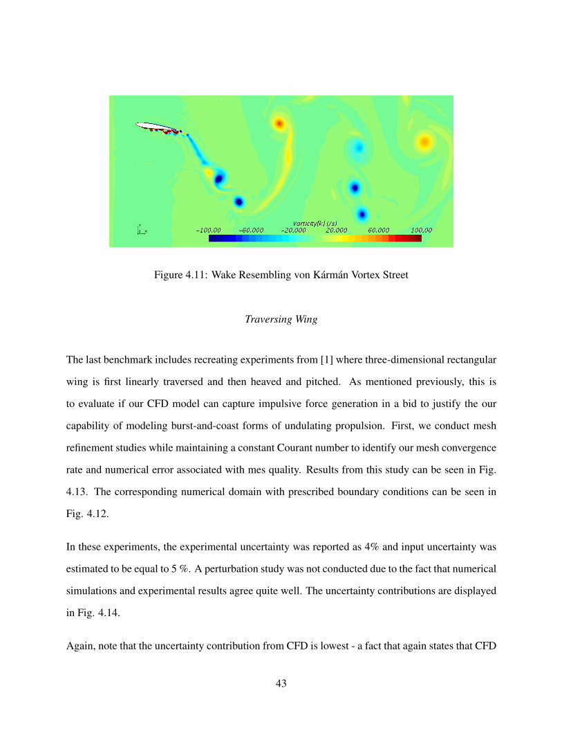
Figure 4.11: Wake Resembling von Kármán Vortex Street

Traversing Wing

The last benchmark includes recreating experiments from [1] where three-dimensional rectangular

wing is first linearly traversed and then heaved and pitched. As mentioned previously, this is

to evaluate if our CFD model can capture impulsive force generation in a bid to justify the our

capability of modeling burst-and-coast forms of undulating propulsion. First, we conduct mesh

refinement studies while maintaining a constant Courant number to identify our mesh convergence

rate and numerical error associated with mes quality. Results from this study can be seen in Fig.

4.13. The corresponding numerical domain with prescribed boundary conditions can be seen in

Fig. 4.12.

In these experiments, the experimental uncertainty was reported as 4% and input uncertainty was

estimated to be equal to 5 %. A perturbation study was not conducted due to the fact that numerical

simulations and experimental results agree quite well. The uncertainty contributions are displayed

in Fig. 4.14.

Again, note that the uncertainty contribution from CFD is lowest - a fact that again states that CFD

43

Figure 4.12: Traversing Wing Numerical Domain

Figure 4.13: Traversing Wing Mesh Refinement Study

is capable of simulating isolated characteristics of undulating propulsion. Comparison results of

Lift and Drag values from the experiments are compared to CFD predictions. Results show excel-

lent agreement In this case, we have validated an impulsively derived motion. With this validation,

we can extrapolate our solution to more complicated geomtries and locomotion kinematics.

44

Numerical Experiment Input Model0.98% 4% 5% 2%

Figure 4.14: Traversing Wing Uncertainties

Figure 4.15: Comparison of Time-Varying Lift

Fluid-Boundary Interactions

Vortex-Foil Interactions

It was previously found [2] that propulsive and efficiency gains are possible when a foil operates

in the wake of a preceding foil. One possible mechanism driving this rise is that the secondary foil

takes advantage of the interaction with a shed vortex from the preceding foil. Due to the oscillatory

nature of the wake of undulating bodies, vortices can either constructively or destructively interact

with a nearby boundary and is supported in previous work [27, 9]. One study evaluated undulating

foils placed in the wake of a D-tube cylinder with systematic changes in distance downstream

[27]. In this study, the phase of the undulating foil was fixed and thus the foil is subject to both

constructive and destructive vortexes.

45

Figure 4.16: Comparison of Time-Varying Drag

In a previous section, the heaving and pitching experiments conducted by [24] were recreated and

validated with the CFD tool set. Following the previous effort of establishing reasonable correla-

tion between the present model and experimental measurements, we move from a single pitching-

heaving NACA 0012 airfoil to a pair of NACA 0012 airfoil pitching and heaving in tandem. The

motions of the two foils are identical and are given by: (1) pitch amplitude of θmax = 25deg, heav-

ing amplitude of A/L = 0.75, and oscillation frequencies (St) varied from 0.1 through 0.4. These

pitch-heave settings correspond to the case where CFD best correlated to experimental measure-

ments. In terms of tandem operation, the leading edge of the second foil was offset by dy = D,

where D = 2A and dx = x/L (see Fig. 4.17) with dx being systematically increased. The x-axis

represents a non-dimensional separation distance (dx/L) from one foil leading edge to another and

the y-axis records the thrust coefficient of the secondary foil.

Results of the mean CT as a function of offset distance are presented in Fig. 4.18. The plot de-

scribes thrust variation with respect to swimming in the wake of a foil as a function of downstream

distance. Note that changes in distance can also correlate to changes in foil phase, hence, relative

vortex interactions can be obtained via swimming further downstream and/or swimming with a

phase lag with respect to the preceding foil. It is interesting to note that the optimal thrust rise

46

Figure 4.17: Foil Separation Schematic

Figure 4.18: Thrust Coefficient vs Foil Separation

decays with distance. This is likely due to vortex dissipation, which is partly associated with nu-

merical dissipation. Nevertheless, the effect leads to CT converging to an average value when the

foil is operating without the effects of an incoming wake. Of particular interest are the peaks as

these indicate how a fish can maximize thrust for a given motion.

In order to better understand CT rises and gains with respect to operation in a wake, the initial

vortex interaction is evaluated in Fig. 4.19. One aspect of this interaction correlates to shear forces

imposed onto the foil. For thrust rises, the vortex rotation contributes a positive shear (or thrust),

versus negative (or drag-direction) shearing when the thrust is reduced. In Fig. 4.19 (a), shows

47

Figure 4.19: Constructive and Destructive Vortex Interaction

the downstream foil is positioned at 1.5L from the leading foil. From Fig. 4.18, this condition

results in a thrust gain. In this interaction, a counter-clockwise vortex occurs on the lower part of

the foil providing a net-thrust rise due to viscous effects. More specifically, the vortex shears the

local foil boundary layer in opposite direction of the flow effectively reducing the drag force on the

foil. Conversely, the opposite effect is observed in the image in Fig. 4.19 (b), which corresponds

to the lowest thrust observed in Fig. 4.18 (at an LE-LE distance of 3.0). In this case the vortex has

the effect of driving a stronger outer velocity of the boundary layer (in the free-stream direction)

consequently leading to an increase in the surface shear force in the drag direction. Note that the

magnitude of the negative affect is lower due to the fact that vortex is both weaker and farther away

from the boundary.

Parametric Studies

The fully undulating foils in tandem are now considered in the context of a schooling configuration.

To consider schooling, recall a "fully developed" interface, which imposes the wake into the inlet

and specifies the pressure drop (rather than velocity). Such a condition evaluates the foils in the

center of a school. In the context of this configuration, parametric studies of the variables displayed

in Fig. 4.20 are performed. The results are evaluated through the CT , which is recorded as a

48

Parameter Range Units IncrementPressure Gradient 100 - 500 Pa 400

Velocity 4 - 6 m/s 2Amplitude 0.05 - 0.1 m 0.05Frequency 1 - 2 1/s 0.5

Wave Speed 2 - 8 1/s 2

Figure 4.20: Parametric Study Variables

time-average value on the both foils using the mean flow velocity on a plane downstream of the

secondary foil (recall that pressure drop and not velocity is specified) and foil reference area.

Two experiments are performed for each case which are: 1) varying parameters for both foils

simultaneously and 2) holding the leading foil motion constant and varying the secondary foil

motion parameters. The parameters are varied as follows: for the schooling scenario, there are two

pressure gradients prescribed. Relative to these two pressure gradients, two amplitudes are also

evaluated. This yields a 2x2 array of plots. Within these plots, the frequency and wave speed are

independently varied to create a contour plot comparing the predicted thrust coefficient (contour),

frequency (x− axis), and wave speed (y− axis). The motion for the cases where the leading foil

motion is not changed is defined by the following parameters: f = 1, A = 0.05, and v = 4. These

parameters were arbitrarily selected so as to focus the analysis on vortex interactions with the

secondary foil.

Figure 4.21 shows thrust coefficient data for a tandem set of foils with a constant leading foil and

varying secondary foil motion. The most noticeable trend is the correlation between increasing

thrust coefficient and increasing wave speed. However, not all frequency values benefit from in-

creases in wave speed as can be seen by examining increases in wave speed when frequency is held

at 2. In fact, at higher frequencies, wave speed negatively impacts performance. We suspect this

is due to the inability of the foil to constructively interact with the shed vortexes from the leading

49

(a) u = 4, A = 0.05 (b) u = 4, A = 0.1

(c) u = 6, A = 0.05 (d) u = 6, A = 0.1

Figure 4.21: Tandem Foil, Secondary Motion Study

foil.

It is possible that due to such a high wave speed, the secondary foil appears to behave as a bluff

body and the vortexes convect around it rather than an undulating foil that vortexes can be captured

by. We can also assume this is the reason why Anguilliform swimmers tend to operate in lower

50

(a) u = 4, A = 0.005 (b) u = 4, A = 0.01

(c) u = 6, A = 0.005 (d) u = 6, A = 0.01

Figure 4.22: Tandem Foil, Concurrent Motion Study

Reynolds number regimes as compared to Carangifrom swimming. The plots suggest that Anguil-

liform motions are most effective at higher frequencies and lower flow velocities and wave speeds.

The effect of amplitude seems to globally increase the thrust coefficient.

Figure. 4.22 shows the same experiment only this time the motion of the leading foil is varied

51

Figure 4.23: Tandem Foil, Secondary Vortex Interaction

identically to that of the secondary foil. We observe a similar thrust coefficient response with

changes in frequency and wave speed. It is interesting to note that both configurations seem to

experience a trough in the mid range frequency and wave speed values. This is most obviously

observable in Fig. 4.21, image (d) and Fig. 4.22, image (c). At this point in time the reasons for

this are not quite understood and warrant further analysis.

Figure 4.23 described how a trailing foil can take advantage of incoming vortexes. Figure 4.23

was recorded with parametric values of u = 6ms/s, A = 0.1, f = 1.5, and v = 8. We can see that

secondary foil has multiple shearing interactions with nearby vorticies which collectively decrease

the local drag force.

Figure 4.24 presents thrust coefficient data for a school of foils with a constant leading foil and

varying secondary foil motion. There is a sharp contrast with this data set compared to the previous

cases. In this scenario, the optimum performance is a hybrid combination of wave speed and

52

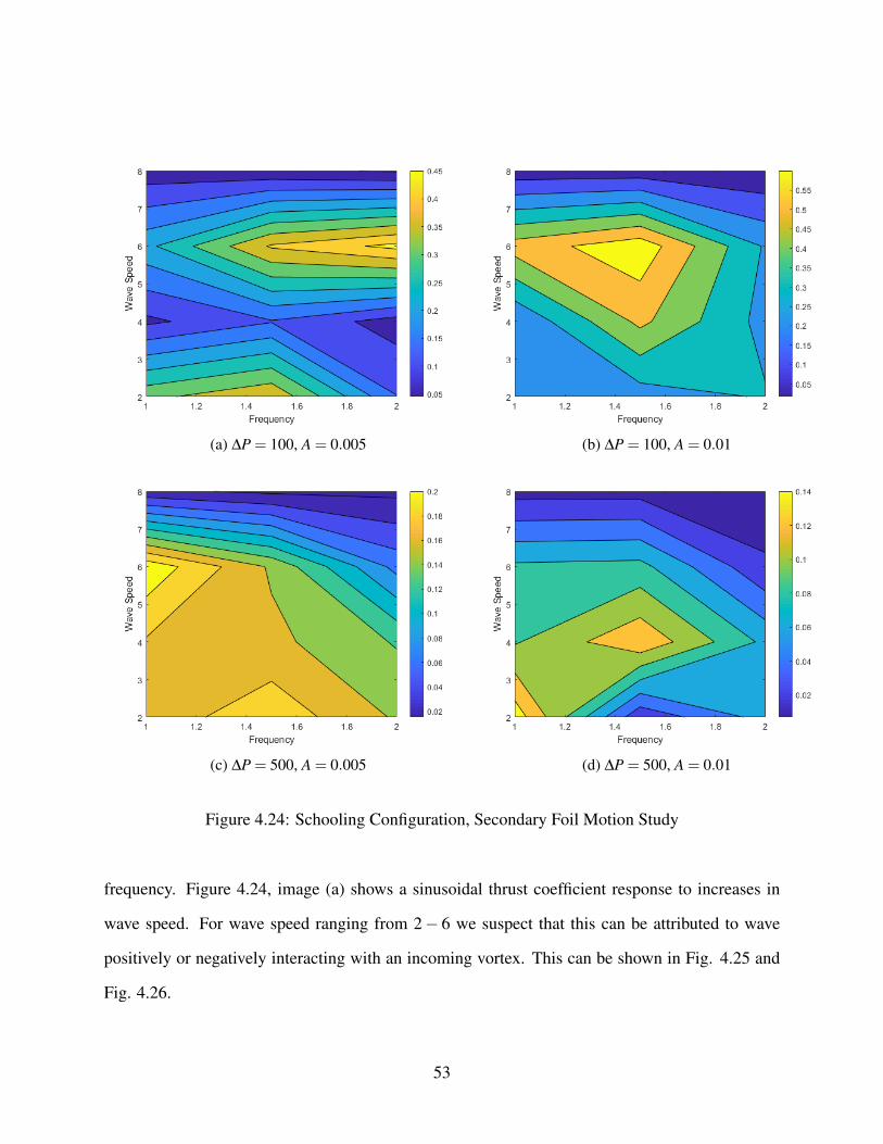
(a) ∆P = 100, A = 0.005 (b) ∆P = 100, A = 0.01

(c) ∆P = 500, A = 0.005 (d) ∆P = 500, A = 0.01

Figure 4.24: Schooling Configuration, Secondary Foil Motion Study

frequency. Figure 4.24, image (a) shows a sinusoidal thrust coefficient response to increases in

wave speed. For wave speed ranging from 2− 6 we suspect that this can be attributed to wave

positively or negatively interacting with an incoming vortex. This can be shown in Fig. 4.25 and

Fig. 4.26.

53

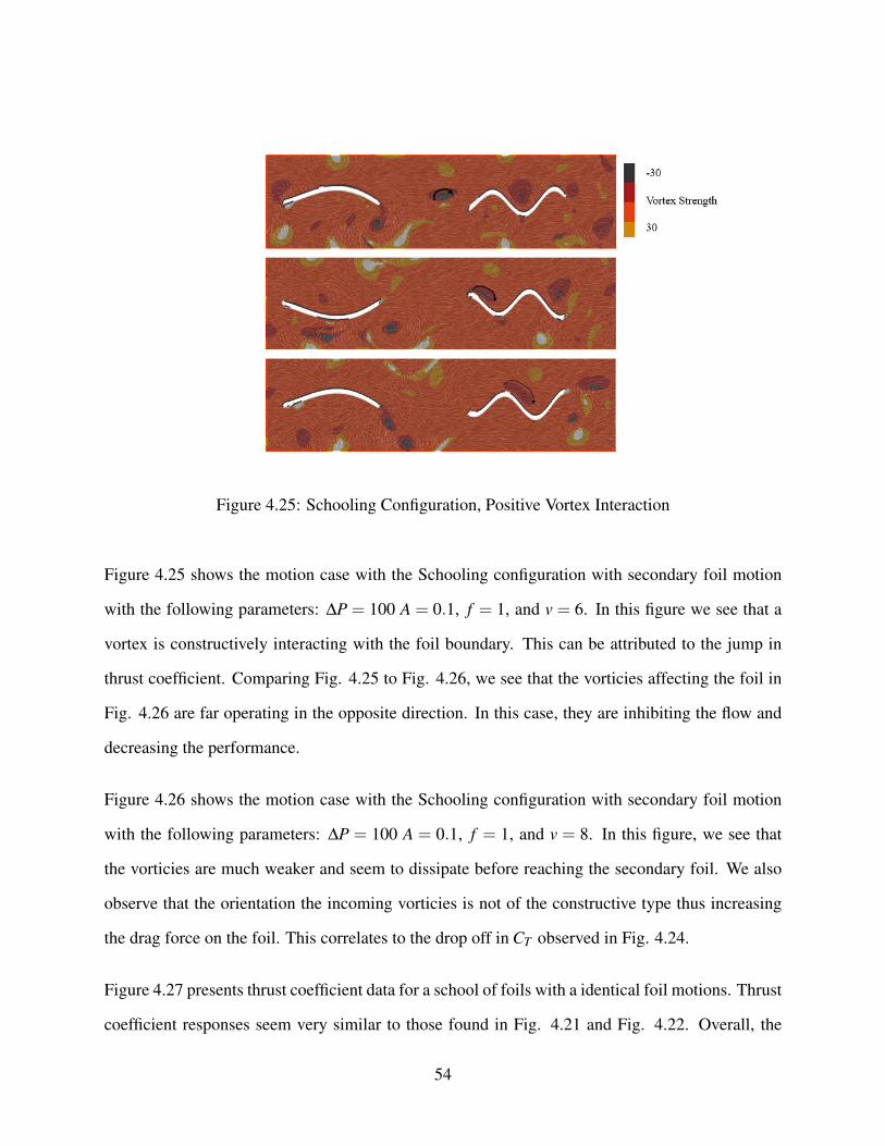
Figure 4.25: Schooling Configuration, Positive Vortex Interaction

Figure 4.25 shows the motion case with the Schooling configuration with secondary foil motion

with the following parameters: ∆P = 100 A = 0.1, f = 1, and v = 6. In this figure we see that a

vortex is constructively interacting with the foil boundary. This can be attributed to the jump in

thrust coefficient. Comparing Fig. 4.25 to Fig. 4.26, we see that the vorticies affecting the foil in

Fig. 4.26 are far operating in the opposite direction. In this case, they are inhibiting the flow and

decreasing the performance.

Figure 4.26 shows the motion case with the Schooling configuration with secondary foil motion

with the following parameters: ∆P = 100 A = 0.1, f = 1, and v = 8. In this figure, we see that

the vorticies are much weaker and seem to dissipate before reaching the secondary foil. We also

observe that the orientation the incoming vorticies is not of the constructive type thus increasing

the drag force on the foil. This correlates to the drop off in CT observed in Fig. 4.24.

Figure 4.27 presents thrust coefficient data for a school of foils with a identical foil motions. Thrust

coefficient responses seem very similar to those found in Fig. 4.21 and Fig. 4.22. Overall, the

54

Figure 4.26: Schooling Configuration, Negative Vortex Interaction

data in these plots suggest that for these swimming motions, isolated tandem swimmers are more

efficient. This can be attributed to the fact that our motion methods were not optimized. This

warrants further investigation to optimize efficiency.

Moment Analysis

In this section we present our moment analysis for two undulating cases. First, we show a time-

averaged scalar plot of the x-velocity component highlighting the jet profile shown in Fig. 4.28.

The most noticeable difference between the wake of the high frequency, low amplitude motion

and the low amplitude, high frequency motion is the shape of the jet-profile. The high frequency,

low amplitude motion has a tight, streamlined jet while the low frequency, high amplitude motion

exhibits a wider jet. Figure 4.29 shows a normalized comparison of the time-averaged velocity

distribution at the integration plane mentioned earlier.

55

(a) ∆P = 100, A = 0.01 (b) ∆P = 100, A = 0.005

(c) ∆P = 500, A = 0.01 (d) ∆P = 500, A = 0.005

Figure 4.27: Schooling Configuration, Concurrent Foil Motion Study

In Fig 4.29, the time-averaged velocity profiles are plotted for both undulating foils in the wake at

a half-chord distance behind the trailing edge. On the x-axis we have the non-dimensional velocity

plotted and on the y-axis we have vertical distance normalized by chord length. We note that both

foils experience viscous losses based on less-than-free-stream velocity regions values in Fig 4.29.

These velocities are slowed down from the free-steam condition are due to viscous interactions with

56

Figure 4.28: Time-Averaged Wake Profiles for Undulating Cases

Figure 4.29: Velocity Distribution in Wake

the no-slip boundary. Thus, we can draw the conclusion that the lower frequency, higher amplitude

motions does in fact experience higher viscous losses due to its specific undulating motion as

compared to the high frequency, low amplitude motion. Using the time-averaged velocity, the

aforementioned shape factors (or moments) can be evaluated.

57

Figure 4.30: Momentum Moments

Figure 4.31: Kinetic Energy Moments

First we discuss the mean values for momentum, kinetic energy, and power. Due to the fact that

both foils are not generating the exact same thrust, it is expected that the mean momentum values

are also not identical. Furthermore, due to the lower frequency, higher amplitude motions produc-

ing a slightly higher thrust we also expect its mean coefficient to be higher as well. In Fig. 4.30,

4.32, both assumptions appear to be validated.

Moving on to the 1st moment or the width factor, we observe that the higher amplitude motion

has a larger width factor then the lower amplitude motion. As shown earlier, this factor directly

58

Figure 4.32: Power Moments

correlates to the width of the velocity distribution. Here, we introduce our power-calculations to

explore this shape factor. Due to the nature of the large amplitude motion for propulsion purposes,

a large frequency is not needed to generate the propulsion. Rather, the large heaving and pitch-

ing based motions generate the the thrust. Therefore, the mechanical power is much lower for a

low frequency, high amplitude case. When examining the inertial terms in the mechanical power

calculations, we can observe that the motion frequency drastically increases this term due to the

inertial terms. Therefore, we draw the correlation that a higher width factor can correlate to a lower

mechanical power when comparing two forms for undulation.

Examining the 3rd moment or the length factor, we again see that the low frequency, high amplitude

motion has a larger length factor. As we concluded previously, this shows that this configuration

has more viscous drag associated with its motion. Again, we can visually observe Fig. 4.29 and

see that there is a large shearing region for the high amplitude, low frequency motion as compared

to the low amplitude, high frequency motion. Thus, we conclude that a higher length factor indi-

cates higher viscous shearing. Using this information, we conclude that the high amplitude, low

frequency case has a higher viscous drag associated with its motion.

59

CHAPTER 5: CONCLUSION

In this presented work, three items were analyzed: developing an accurate numerical model based

on a verification and validation approach, conducting numerical investigations to increase under-

standing of undulating propulsion in the context of unsteady fluid interactions, and developing a

new method for evaluating undulating propulsion by examining wake profiles. In the following

sections, we will discuss conclusions for each item.

Verification and Validation

In this analysis, a verification and validation study with respect to numerically simulating propul-

sion is conducted. Specifically, three relevant experiments are simulated in CFD and compared to

experimental results. These experiments include measuring vortex shedding frequencies behind a

D-tube, measuring thrust from a heaving and pitching foil, and measuring forces on a 3D traversing

and pitching wing. These experiments have been selected for validation because they posses fluid

characteristics that are representative of fluid dynamics associated with undulating propulsion.

As seen in the comparison between experimental and simulated data, there are discrepancies in the

numerical tool sets capability to predict physics associated with undulating propulsion. However,

when considering the uncertainty contributions, it is evident that these discrepancies are dominated

by experimental techniques and are not dominated by numerical error. Hence, we can definitively

state that the numerical model has been verified and validated, and is ready to be used for future

numerical experimentation.

60

Numerical Experiments

In this analysis we analyzed multiple cases of undulation based propulsion to develop an under-

standing the key parameters responsible. Our parametric studies have revealed that vortex shearing

plays an inherent role in aiding or retarding thrust generation. Based on the rotation of a vortex

interacting with a foil boundary, vortex shearing can be positive or negative. This was hypoth-

esis was validated by varying the off-set distance of two NACA airfoils while allowing them to

heave and pitch. Furthermore, when examining tandem and schooling configurations, we observed

a steep change in thrust generation based on the orientation of the local vortex with respect to a

nearby boundary.

Our analysis also showed a correlation between thrust generation, motion frequency, and ampli-

tude. For a tandem foil configuration, we find that the highest thrust generation is generated when

a low frequency and high wave speed is used. We hypothesize that is due to less flow turning

and therefore less shearing due to vortex generation. While constructive vortex interactions are

beneficial to secondary thrust generation, an optimization problem is present.

Moment Analysis

In this analysis, wake profiles are used to explore, compare, and evaluate two undulating NACA

0012 foils. Specifically, these two foils use different motions schemes; one being high frequency

and low amplitude displacement and the second being an inverse for the first. In both cases, the two

motions generate the nearly same thrust that is greater than its drag. This was enforced to standard-

ize the foils and focus the analysis on the efficiency of each propulsion method. By enforcing this

condition, we were able to interrogate our analysis approach. The mechanical power required to

generate each specific motion was also evaluated which yielded more information when examining

61

foil moments, and allowed us to draw more refined correlations. To baseline our analysis, we inter-

rogated moments for two static NACA 0012 foils; a standard foil and one with double thickness.

Due to the simplicity of this problem and known performance data, we established preliminary

shape factor relations before exploring undulating cases.

From these studies and approaches, several insights can be drawn. When comparing the 0th shape

factor or mean of the time-averaged velocity distribution, we see that a higher moment represents

a larger thrust (respective to momentum). When examining the kinetic energy and power cases,

we can infer similar trends, mainly, that difference in the mean moment correlates to higher kinetic

energy and power in the wake. When examining the 1st moment or the width factor, we can see that

this yields information on the shape of the thrust (when examining momentum). This conclusion

was validated by analyzing the static NACA foils. When comparing undulating motions, we can

see that this correlates to the amplitude term. Due to the thrust being relatively constant for both

foils, we infer that a larger amplitude term corresponds to a lower frequency. Therefore, we now

can relate the 1st moment to the mechanical power of the system where a higher 1st moment

represents lower mechanical power for undulating motions. With regards to the 3rd moment of the

length factor we showed that this correlates to viscous shearing. Following our previous discussion,

we conclude that a larger length factor indicates higher viscous shearing when comparing two

motions.

Future Work

Within the scope of this work, there are numerous objectives that can still be researched. One such

a objective could be analyzing 2-way coupled simulations which take into consideration the struc-

tural properties of swimmers. Research in this field could reveal if there any trade-offs between

improved structural qualities and hydrodynamic efficiencies. This would likely play an important

62

role when incorporating undulating propulsion into marine propulsion. Another area of interest re-

volves around expanding our modeling methods to fully three-dimensional simulations. Examples

of this include marine swimmers such as sting ray which are exposed to induced flow effects.

63

LIST OF REFERENCES

[1] Dibya Raj Adhikari et al. “Unsteady Ground Effects On A Rectangular And Swept Wing

Undergoing Heaving And Pitching During Deceleration”. In: AIAA Scitech 2020 Forum.

2020, p. 0334.

[2] Imran Akhtar et al. “Hydrodynamics of a biologically inspired tandem flapping foil config-

uration”. In: Theoretical and Computational Fluid Dynamics 21.3 (2007), pp. 155–170.

[3] JM Anderson et al. “Oscillating foils of high propulsive efficiency”. In: Journal of Fluid

mechanics 360 (1998), pp. 41–72.

[4] A Betz. “Zeitschrift Faur Flugtechnik Und Motorluftschiffahrt”. In: Beitrag Zur Erklarung

Des Segelfluges 3 (1912), pp. 269–272.

[5] Iman Borazjani and Fotis Sotiropoulos. “Numerical investigation of the hydrodynamics of

carangiform swimming in the transitional and inertial flow regimes”. In: Journal of experi-

mental biology 211.10 (2008), pp. 1541–1558.

[6] Cesar Cantu, Benito Gonzalez, and Sanjay Kumar. “An Experimental Study of Flow Around

a Spinning Cylinder”. In: APS Division of Fluid Dynamics Meeting Abstracts. 2009.

[7] Jian-Yu Cheng and Georges L Chahine. “Computational hydrodynamics of animal swim-

ming: boundary element method and three-dimensional vortex wake structure”. In: Com-

parative Biochemistry and Physiology Part A: Molecular & Integrative Physiology 131.1

(2001), pp. 51–60.

[8] Christopher J Freitas. “The issue of numerical uncertainty”. In: Applied Mathematical Mod-

elling 26.2 (2002), pp. 237–248.

64

[9] Amy Gao and Michael S Triantafyllou. “Independent caudal fin actuation enables high en-

ergy extraction and control in two-dimensional fish-like group swimming”. In: Journal of

Fluid Mechanics 850 (2018), pp. 304–335.

[10] Thomas Geyer, Ennes Sarradj, and Christoph Fritzsche. “Silent owl flight: comparative

acoustic wind tunnel measurements on prepared wings”. In: Acta Acustica United with Acus-

tica 99.1 (2013), pp. 139–153.

[11] Hongyi Jiang and Liang Cheng. “Strouhal–Reynolds number relationship for flow past a

circular cylinder”. In: Journal of Fluid Mechanics 832 (2017), pp. 170–188.

[12] Marleen Kamperman et al. “Functional adhesive surfaces with “gecko” effect: The concept

of contact splitting”. In: Advanced Engineering Materials 12.5 (2010), pp. 335–348.

[13] Asimina Kazakidi et al. “CFD study of aquatic thrust generation by an octopus-like arm

under intense prescribed deformations”. In: Computers & Fluids 115 (2015), pp. 54–65.

[14] Culbert B Laney. Computational gasdynamics. Cambridge university press, 1998.

[15] James C Liao et al. “The Kármán gait: novel body kinematics of rainbow trout swimming

in a vortex street”. In: Journal of experimental biology 206.6 (2003), pp. 1059–1073.

[16] Michael James Lighthill. “Large-amplitude elongated-body theory of fish locomotion”. In:

Proceedings of the Royal Society of London. Series B. Biological Sciences 179.1055 (1971),

pp. 125–138.

[17] Audrey P Maertens, Amy Gao, and Michael S Triantafyllou. “Optimal undulatory swim-

ming for a single fish-like body and for a pair of interacting swimmers”. In: Journal of

Fluid Mechanics 813 (2017), pp. 301–345.

[18] S R Mathur and J Y Murthy. “A pressure-based method for unstructured meshes”. In: Nu-

merical Heat Transfer 31.2 (1997), pp. 195–215.

65

[19] American Society of Mechanical Engineers. Standard for Verification and Validation in

Computational Fluid Dynamics and Heat Transfer: An American National Standard. Amer-

ican Society of Mechanical Engineers, 2009.

[20] Keith W Moored. “Unsteady three-dimensional boundary element method for self-propelled

bio-inspired locomotion”. In: Computers & Fluids 167 (2018), pp. 324–340.

[21] Ulrike K Müller et al. “How the body contributes to the wake in undulatory fish swimming:

flow fields of a swimming eel (Anguilla anguilla)”. In: Journal of Experimental Biology

204.16 (2001), pp. 2751–2762.

[22] Michael P Murphy et al. “Waalbot II: Adhesion recovery and improved performance of a

climbing robot using fibrillar adhesives”. In: The International Journal of Robotics Research

30.1 (2011), pp. 118–133.

[23] Chen Rao et al. “Owl-inspired leading-edge serrations play a crucial role in aerodynamic

force production and sound suppression”. In: Bioinspiration & biomimetics 12.4 (2017),

p. 046008.

[24] Douglas A Read, FS Hover, and MS Triantafyllou. “Forces on oscillating foils for propul-

sion and maneuvering”. In: Journal of Fluids and Structures 17.1 (2003), pp. 163–183.

[25] Patrick J Roache, Kirti N Ghia, and Frank M White. Editorial policy statement on the control

of numerical accuracy. 1986.

[26] Hermann Schlichting. Boundary layer theory. Vol. 960. Springer, 1960.

[27] Xueming Shao et al. “Hydrodynamic performance of a fishlike undulating foil in the wake

of a cylinder”. In: Physics of Fluids 22.11 (2010), p. 111903.

[28] Kourosh Shoele and Qiang Zhu. “Fluid–structure interactions of skeleton-reinforced fins:

performance analysis of a paired fin in lift-based propulsion”. In: Journal of Experimental

Biology 212.16 (2009), pp. 2679–2690.

66

[29] STAR CCM+ Users Manual. 2018.

[30] Federico La Torre et al. “Effects of wavy surface roughness on the performance of micronoz-

zles”. In: Journal of Propulsion and Power 26.4 (2010), pp. 655–662.

[31] JJ Videler and D Weihs. “Energetic advantages of burst-and-coast swimming of fish at high

speeds”. In: Journal of Experimental Biology 97.1 (1982), pp. 169–178.

[32] David W Weyburne. “New thickness and shape parameters for the boundary layer velocity

profile”. In: Experimental Thermal and Fluid Science 54 (2014), pp. 22–28.

[33] Frank M White and Isla Corfield. Viscous fluid flow. Vol. 3. McGraw-Hill New York, 2006.

[34] Guanhao Wu, Yan Yang, and Lijiang Zeng. “Kinematics, hydrodynamics and energetic ad-

vantages of burst-and-coast swimming of koi carps (Cyprinus carpio koi)”. In: Journal of

Experimental Biology 210.12 (2007), pp. 2181–2191.

[35] Yan Yang et al. “A study on flow physics of burst-and-coast swimming of koi carp (Cyprinus

carpio koi) based on measurements and numerical simulations”. In: Journal of Aero Aqua

Bio-mechanisms 1.1 (2010), pp. 30–38.

[36] Zhang Yong-Hua, He Jian-Hui, and Low Kin-Huat. “Numeric simulation on the perfor-

mance of an undulating fin in the wake of a periodic oscillating plate”. In: International

Journal of Advanced Robotic Systems 10.10 (2013), p. 352.

[37] Cheng-Lun Yu et al. “Three-dimensional numerical simulation of hydrodynamic interac-

tions between pectoral-fin vortices and body undulation in a swimming fish”. In: Physics of

Fluids 23.9 (2011), p. 091901.

67