Efficient Collision Detection Using Bounding VolumeHierarchies of k-DOPs�

James T. Klosowski y Martin Held z Joseph S.B. Mitchell x Henry Sowizral {

Karel Zikan k

Abstract – Collision detection is of paramount importance for many applications in computer graphics and visual-ization. Typically, the input to a collision detection algorithm is a large number of geometric objects comprising anenvironment, together with a set of objects moving within the environment. In addition to determining accurately thecontacts that occur between pairs of objects, one needs also to do so at real-time rates. Applications such as hapticforce-feedback can require over 1000 collision queries per second.

In this paper, we develop and analyze a method, based on bounding-volume hierarchies, for efficient collisiondetection for objects moving within highly complex environments. Our choice of bounding volume is to use a “discreteorientation polytope” (“k-dop”), a convex polytope whose facets are determined by halfspaces whose outward normalscome from a small fixed set of k orientations. We compare a variety of methods for constructing hierarchies (“BV-trees”) of bounding k-dops. Further, we propose algorithms for maintaining an effective BV-tree of k-dops for movingobjects, as they rotate, and for performing fast collision detection using BV-trees of the moving objects and of theenvironment.

Our algorithms have been implemented and tested. We provide experimental evidence showing that our approachyields substantially faster collision detection than previous methods.

Index Terms – Collision detection, intersection searching, bounding volume hierarchies, discrete orientation poly-topes, bounding boxes, virtual reality, virtual environments.

To appear in the March issue (Vol. 4, No. 1) of IEEE Transactions on Visualization and Computer Graphics.

c 1998 IEEE. Personal use of this material is permitted. However, permission to reprint/republish this material for advertising or promotional

purposes or for creating new collective works for resale or redistribution to servers or lists, or to reuse any copyrighted component of this work in

other works must be obtained from the IEEE.

�A technical sketch of this paper appeared in the SIGGRAPH’96 Visual Proceedings [26].yjklosow@ams.sunysb.edu; http://www.ams.sunysb.edu/˜jklosow/jklosow.html. Department of Applied Mathematics and Statistics, State Uni-

versity of New York, Stony Brook, NY 11794-3600. Supported by NSF grant CCR-9504192, and by grants from Boeing Computer Services,Bridgeport Machines, and Sun Microsystems. Also partially supported by a Catacosinos Fellowship.

zheld@ams.sunysb.edu; http://www.ams.sunysb.edu/˜held/held.html. Department of Applied Mathematics and Statistics, State University ofNew York, Stony Brook, NY 11794-3600. Supported by NSF grants DMS-9312098 and CCR-9504192, and by grants from Boeing ComputerServices, Bridgeport Machines, and Sun Microsystems.

xjsbm@ams.sunysb.edu; http://www.ams.sunysb.edu/˜jsbm/jsbm.html. Department of Applied Mathematics and Statistics, State University ofNew York, Stony Brook, NY 11794-3600. Partially supported by NSF grant CCR-9504192, and by grants from Boeing Computer Services,Bridgeport Machines, Hughes Aircraft, and Sun Microsystems.

{henry.sowizral@eng.sun.com; Sun Microsystems, 2550 Garcia Avenue, UMPK14-202, Mountain View, CA 94043-1100.kzikan@fi.muni.cz; Faculty of Informatics, Masaryk University, Botanicka 68a, Brno, Czech Republic. Part of this research was conducted

while being supported by a Fulbright Scholars Award.

1 Introduction

The collision detection (CD) problem takes as input a geometric model of a scene or environment (e.g., a large col-lection of complex CAD models), together with a set of one or more moving (“flying”) objects, possibly articulated,and asks that we determine all instants in time at which there exists a nonempty intersection between some pair offlying objects, or between a flying object and an environment model. Usually, we are given some information abouthow the flying objects are moving, at least at the current instant in time; however, the motions may change rapidly,depending on the evolution of a simulation (e.g., modeling some physics of the system), or due to input devices undercontrol of the user. In some applications, it is important to make computations based on the geometry of the regionof intersection between pairs of colliding objects; in these cases, we must not only detect that a collision occurs, butalso report all pairs of primitive geometric elements (e.g., triangles) that are intersecting at that instant. Thus, we candistinguish between the CD problem of pure detection and the CD problem of detect and report.

Real-time collision detection is of critical importance in computer graphics, visualization, simulations of physicalsystems, robotics, solid modeling, manufacturing, and molecular modeling. The requirement for speed in interactiveuse of virtual environments is particularly challenging; e.g., haptic force-feedback can require on the order of 1000intersection queries per second. One may, for example, wish to interact with a virtual world that models a cluttered me-chanical workspace, and ask how easily one can assemble, access, or replace component parts within the workspace:Can a particular subassembly be removed without collisions with other parts, and while not requiring undue awkward-ness for the mechanic? When using haptic force-feedback, the mechanic is not only alerted (e.g., audibly or visually)about a collision, but actually feels a reactionary force, exerted on his body by a haptic device.

A simple-minded approach to CD involves comparing all pairs of primitive geometric elements. This methodquickly becomes infeasible as the model complexity rises to realistic sizes. Thus, many approaches have recently beenproposed to address the issue of efficiency; we discuss these below.

Our Contribution. In this paper, we present a new approach to CD, based on a form of bounding volume hierarchy(“BV-tree”). Our main contributions include:

1. a careful study of effective methods of constructing BV-trees, using “discrete orientation polytopes” (“k-dops”);

2. an effective method for applying BV-trees of k-dops for moving (rotating) objects, as well as an efficient algo-rithm, using BV-trees, for detecting collisions1, as objects move within a complex static environment; and

3. experimental results, with real and simulated data, to study design issues of BV-trees that are most relevant tocollision detection.

We have paid careful attention to the generation of particularly challenging and diverse datasets for algorithm designand for comparative studies. Our tests provide experimental evidence that our methods compare quite favorably withthe best previous methods.

This paper is accompanied by supplementary material on the WWW, including additional color photos, sampledatasets, and the (soon to be released) source code; refer to the authors’ web pages.

The remainder of the paper is organized as follows: Prior and related work is reviewed in Section 2. Section 3provides an introduction to BV-trees, discrete orientation polytopes, and design choices in constructing effective BV-trees. Section 4 highlights our collision detection algorithm and several key issues related to it. Implementation detailsand experimental results are reported in Section 5. The conclusion, Section 6, includes a discussion of extensions andfuture work.

2 Previous Work

Due to its widespread importance, there has been an abundance of work on the problem of collision detection. Manyof the approaches have used hierarchies of bounding volumes or spatial decompositions to address the problem. Theidea behind these approaches is to approximate the objects (with bounding volumes) or to decompose the space they

1Strictly speaking, we check for intersections among surfaces rather than volumes. Thus, if one object contains another object but their surfacesdo not intersect, then “no collision” is reported by our algorithm.

1

occupy (using decompositions), to reduce the number of pairs of objects or primitives that need to be checked forcontact.

Octrees [33, 35], k-d trees [24], BSP-trees [34], brep-indices [8, 42], tetrahedral meshes [24], and (regular)grids [19, 24] are all examples of spatial decomposition techniques. By dividing the space occupied by the objects,one needs to check for contact between only those pairs of objects (or parts of objects) that are in the same or nearbycells of the decomposition. Using such decompositions in a hierarchical manner (as in octrees, BSP-trees, etc.) canfurther speed up the collision detection process.

Hierarchies of bounding volumes have also been a very popular technique for collision detection algorithms. (Theyhave also been widely used in other areas, e.g., ray tracing [1, 20, 29, 44].) In building hierarchies on objects, onecan obtain increasingly more accurate approximations of the objects, until the exact geometry of the object is reached.The choice of bounding volume has often been to use spheres [27, 28, 37] or axis-aligned bounding boxes (AABBs)[7, 24], due to the simplicity in checking two such volumes for overlap (intersection). In addition, it is simple totransform these volumes as an object rotates and translates.

Another bounding volume that has become popular recently is the oriented bounding box (OBB), which surroundsan object with a bounding box (hexahedron with rectangular facets) whose orientation is arbitrary with respect to thecoordinate axes; cf. Fig. 1(b). This volume has the advantage that it can, in general, yield a better (tighter) outerapproximation of an object, as its orientation can be chosen in order to make the volume as small as possible. In 1981,Ballard [2] created a two-dimensional hierarchical structure, known as a “strip tree,” for approximating curves, basedon oriented bounding boxes in the plane. Barequet et al. [6] have recently generalized this work to three dimensions(resulting in a hierarchy of OBBs known as a “BOXTREE”), for applications of oriented bounding boxes for fastray tracing and collision detection. Zachmann and Felger [45, 46] have used a similar term, “BoxTree”, for theirhierarchies of oriented boxes, which are also used for collision detection, but are differently constructed from the“BOXTREE” of Barequet et al.

One leading system publicly available for performing collision detection among arbitrary polygonal models is the“RAPID” system, which is also based on a hierarchy of oriented bounding boxes, called “OBBTrees”, implementedby Gottschalk, Lin, and Manocha [21]. The efficiency of this method is due in part to an algorithm for determiningwhether two oriented bounding boxes overlap. This algorithm is based on examining projections along a small set of“separating axes” and is claimed to be an order of magnitude faster than previous algorithms. (We note that Greene[22] previously published a similar algorithm; however, we are not aware of any empirical comparisons between thetwo algorithms.)

Other approaches to collision detection have included using space-time bounds [27] and four-dimensional geom-etry [9, 10] to bound the positions of objects within the near future. By using a fourth dimension to represent thesimulation time, contacts can be pin-pointed exactly; however, these methods are restrictive in that they require themotion to be pre-specified as a closed-form function of time. Hubbard’s space-time bounds [27] do not have sucha requirement; by assuming a bound on the acceleration of objects, he is able to avoid missing collisions betweenfast-moving objects.

There has been a collection of innovative work which utilizes Voronoi diagrams [11, 30, 31, 32] to keep track of theclosest features between pairs of objects. One popular system, I-COLLIDE [11], uses spatial and temporal coherencein addition to a “sweep-and-prune” technique to reduce the pairs of objects that need to be considered for collision.Although this software works well for many simultaneously moving objects, the objects are restricted to be convex.More recently, Ponamgi, Manocha, and Lin have generalized this work to include non-convex objects [38].

In addition to the “practical” work highlighted above, there have also been a considerable number of “theoretical”results on the problem of collision detection in the field of computational geometry. In particular, the distance (andthus intersection) between two convex polytopes can be determined in O(log 2 n), where n is the total number ofvertices of the polytopes, by using the Dobkin-Kirkpatrick hierarchy [15, 16, 17], which takes O(n) time and space toconstruct. In the case of one convex polytope and one non-convex polytope, the intersection detection time increasesto O(n log n) [14, 40], while actually computing the intersection [18] takes O(K logK) time, where K is the size ofthe input plus output. Schomer [40] detects the intersection between two translating “c-iso-oriented” polyhedra (non-convex, having normals among c directions, where c is a fixed constant) in time O(n 5=3+�), for any fixed positiveconstant � > 0. Schomer and Thiel [41] have recently provided the first provably (worst case) sub-quadratic timealgorithm for a general collection of polyhedra in motion along fixed trajectories. However, the result is purely oftheoretical interest, as the methods are based on several sophisticated (unimplemented) techniques.

Recently, Suri, Hubbard, and Hughes [43] have given theoretical results that may help to explain the practicality of

2

bounding volume methods, such as our own. In particular, they show that in a collection of objects that have boundedaspect ratio and scale factor2, the number of pairs of objects whose bounding volumes intersect is roughly proportional,asymptotically, to the number of pairs of objects that actually intersect, plus the number of objects. Suri et al. use thisresult to obtain an output-sensitive algorithm for detecting all intersections among a set of convex polyhedra, havingbounded aspect ratio and scale factor; their time bound is O((n + k) log 2 n), for n polyhedra, where k is the numberof pairs of polyhedra that actually intersect.

3 BV-Trees

We assume as input a set S of n geometric “objects”, which, for our purposes, are generally expected to be triangles in3D that specify the boundary of some polygonal models. Much of our discussion, though, applies also to more generalobjects.

A BV-tree is a tree, BVT(S), that specifies a bounding volume hierarchy on S. Each node, �, of BVT(S) corre-sponds to a subset, S� � S, with the root node being associated with the full set S. Each internal (non-leaf) node ofBVT(S) has two or more children; the maximum number of children for any internal node of BVT(S) is called thedegree of BVT(S), denoted by Æ. The subsets of S that correspond to the children of node � form a partition of theset S� of objects associated with �. In a complete BV-tree of S, the leaf nodes are associated with singleton subsets ofS. The total number of nodes in BVT(S) is at most 2n� 1; the height of a complete tree is at least dlog Æ ne, which isachieved if the BV-tree is balanced. Also associated with each node � of BVT(S) is a bounding volume, b(S �), that isan (outer) approximation to the set S� using a smallest instance of some specified class of shapes (e.g., boxes, spheres,polytopes of a given class, etc.).

In most of this paper, we will be focusing on the case of a single (rigid) object, specified by a set F of boundaryprimitives (triangles), given in one particular position and orientation, that is moving (“flying”) within an environment,specified by a set E of “obstacle” primitives (triangles). We refer to BVT(F ) as the flying hierarchy and BVT(E) asthe environment hierarchy.

3.1 Design Criteria

The choice of which class (or classes) of shapes to use as bounding volumes in a BV-tree is usually dependent uponthe application domain and the different constraints inherent to it. In ray tracing, for example, the bounding volumeschosen should tightly fit the primitive objects but also allow for efficient intersection tests between a ray and thebounding volumes [29]. Weghorst, Hooper, and Greenberg [44] discussed making this choice for ray tracing, andthey provided a cost function to help analyze hierarchical structures of bounding volumes. Gottschalk, Lin, andManocha [21] looked at this same cost function in the context of collision detection. Given two large input modelsand hierarchies built to approximate them, the total cost to check the models for intersection was quantified as

T = Nv � Cv +Np � Cp; (1)

where T is the total cost function for collision detection, Nv is the number of pairs of bounding volumes tested foroverlap,Cv is the cost of testing a pair of bounding volumes for overlap,N p is the number of pairs of primitives testedfor contact, and Cp is the cost of testing a pair of primitives for contact.

While Equation 1 is a reasonable measure of the cost associated with performing a single intersection detectioncheck, it does not take into account the cost of updating the flying hierarchy as the flying object rotates. While for somechoices of bounding volumes (e.g., spheres), there is little or no cost associated with updating the flying hierarchy, ingeneral there will be such a cost, and, in particular, we experience an update cost for our choice (k-dops). Thus, wepropose that for collision detection in motion simulation that the cost is best written as the sum of three componentterms:

T = Nv � Cv +Np � Cp +Nu � Cu; (2)

where T , Nv, Cv , Np, and Cp are defined as in Equation 1, while Nu is the number of nodes of the flying hierarchythat must be updated, and Cu is the cost of updating each such node.

2The aspect ratio of an object is defined here to be the ratio between the volume of a smallest enclosing sphere and a largest enclosed sphere.The scale factor for the collection of objects is the ratio between the volume of the largest enclosing sphere and the smallest enclosing sphere.

3

Based upon this cost function, we would like our bounding volumes to (a) approximate tightly the input primitives(to lower Nv , Np, and Nu), (b) permit rapid intersection tests to determine if two bounding volumes overlap (tolower Cv), and (c) be updated quickly when the primitives (and consequently the bounding volumes) are rotated andtranslated in the scene (to lower Cu). Unfortunately, these objectives usually conflict, so a balance among them mustbe reached.

3.2 Discrete Orientation Polytopes

Here, we concentrate on our experience with bounding volumes that are convex polytopes whose facets are deter-mined by halfspaces whose outward normals come from a small fixed set of k orientations. For such polytopes, wehave coined the term discrete orientation polytopes, or “k-dops”, for short. 3 See Fig. 1(c) for an illustration in twodimensions of an 8-dop, whose 8 fixed normals are determined by the orientations at �45, �90, �135, and �180degrees. Axis-aligned bounding boxes (in 3D) are 6-dops, with orientation vectors determined by the positive andnegative coordinate axes. In this paper, we concentrate on 6-dops, 14-dops, 18-dops, and 26-dops, defined by orienta-tions that are particularly natural; see Section 3.3.3 for more detail.

Researchers at IBM have used the same 18-dops (which they call “tri-boxes” or “T-boxes”) for visual approxima-tion purposes within 3DIX [12, 13]. This idea of using planes of fixed orientations to approximate a set of primitiveobjects was first introduced in the ray tracing work of Kay and Kajiya [29].

(a) AABB (b) OBB (c) 8-dop

Fig. 1: Approximations of an object by three bounding volumes: an axis-aligned bounding box (AABB), an orientedbounding box (OBB), and a k-dop (where k = 8).

Axis-aligned bounding boxes (AABBs) are often used in hierarchies because they are simple to compute and theyallow for very efficient overlap queries. But AABBs can also be particularly poor approximations of the set that theybound, leaving large “empty corners”; consider, for example, a needle-like object that lies at a 45-degree orientationto the axes. Using k-dops, for larger values of k, allows the bounding volume to approximate the convex hull moreclosely. Of course, the improved approximation (which tends to lowerN v, Np, andNu) comes at the cost of increasingthe cost, Cv , of testing a pair of k-dops for intersection (since Cv = O(k)) and the cost, Cu, of updating k-dops in theflying hierarchy (since Cu = O(k2)).

To keep the associated costs as small as possible, we have been using only k-dops whose discrete orientationnormals come as pairs of collinear, but oppositely oriented, vectors. Kay and Kajiya referred to such pairs as boundingslabs [29]. Thus, as an AABB bounds (i.e., finds the minimum and maximum values of) the primitives in the x, y,and z directions, our k-dops will also bound the primitives but in k=2 directions. This has the advantage in that our(conservative) disjointness test for two k-dops is essentially as trivial as checking two AABBs for overlap: we simplyperform k=2 interval overlap tests. This test is far simpler than checking for intersection between OBBs or betweenconvex hulls. Further, since the k=2 defining directions are fixed, the memory required to store each k-dop is only kvalues (one value per plane), since the orientations of the planes are known in advance.

3An alternative name for what we call a “dop” is the term fixed-directions hull [47] (FDH)—perhaps a slightly more precise term, but a harderto pronounce abbreviation.

4

Bounding spheres are another natural choice to approximate an object, since it is particularly simple to test pairsfor overlap, and the update for a moving object is trivial. However, spheres are similar to AABBs in that they can bevery poor approximations to the convex hull of the contained object. Hence, bounding spheres yield low costs C v andCu, but may result in a large number, Np, of pairs of primitives to test. Oriented bounding boxes (OBBs) can yieldmuch tighter approximations than spheres and AABBs, in some cases. Also, it is relatively simple to update an OBB,by multiplying two transformation matrices. However, the cost C v for determining if two OBBs overlap is roughlyan order of magnitude larger than for AABBs [21]. At the extreme, convex hulls provide the tightest possible convexbounding volume; however, both the test for overlap and the update costs are relatively high.

In comparison, our choice of k-dops for bounding volumes is made in hopes of striking a compromise between therelatively poor tightness of bounding spheres and AABBs, and the relatively high costs of overlap tests and updatesassociated with OBBs and convex hulls. The parameter k allows us some flexibility too in striking a balance betweenthese competing objectives. For moderate values of k, the cost C v of our conservative disjointness test is an orderof magnitude faster than testing two OBBs. Also, while updating a k-dop for a rotating object is more complexthan updating some other bounding volumes, we have developed a simple approximation approach, discussed inSection 4.1, that works well in practice.

Fig. 1 highlights the differences in some of the typical bounding volumes. Here, we provide a simple two-dimensional illustration of an object and its corresponding approximations by an axis-aligned bounding box (AABB),an oriented bounding box (OBB), and a k-dop (where k = 8).

3.3 Design Choices

Our study has included a comparison of various design choices in constructing BV-trees, including: (1) the degree, Æ,of the tree (binary, ternary, etc.); (2) top-down versus bottom-up construction; (3) the choice of the k-dops; and (4)splitting rules.

3.3.1 Degree of the Tree

Minimizing the height of the tree is usually a desirable quality when building a hierarchy, so that when searches areperformed, we can traverse the tree, from the root to a leaf, in a small number of steps. The degree, Æ, specifies themaximum number of children any node can have. Typically, the higher the degree, the smaller the height of the tree.There is, of course, a trade-off between trees of high and low degree. A tree with a high degree will tend to be shorter,but more work will be expended per node of the search. On the other hand, a low-degree tree will have greater height,but less work will be expended per node of the search.

We have chosen to use binary (Æ = 2) trees for all of the experiments reported herein, for two reasons. First, theyare simpler and faster to compute, since there are fewer options in how one splits a set in two than how one partitionsa set into three or more subsets. Second, analytical evidence suggests that binary trees are better than Æ-ary trees, forÆ > 2. In particular, if one considers balanced trees (with n leaves) whose internal nodes have degree Æ � 2, thenthe amount of work expended in searching a single path from root to leaf is proportional to f(Æ) = (Æ � 1) � log Æ n,since at most Æ � 1 of the Æ children need to be tested before we know how to descend. Simple calculus shows thatthe function f(Æ) is monotonically increasing over the interval Æ 2 (1;1) (and f 0(1) = 0). Restricting Æ to integervalues greater than one, we see that f(Æ) is minimized by Æ = 2. Of course, this analysis does not address the factthat a typical search of a BV-tree will not consist of a single root-to-leaf path. However, from our limited investigationof some typical searches, we have found that our choice of Æ = 2 is justified. We leave for future work the thoroughexperimental investigation of the trade-offs between different values of Æ.

3.3.2 Top-Down versus Bottom-Up

In constructing a BV-tree on a set, S, of input primitives, we can do so in either a top-down or a bottom-up manner.A bottom-up approach begins with the input primitives as the leaves of the tree and attempts to group them togetherrecursively (taking advantage of any local information), until we reach a single root node which approximates theentire set S. One example of this approach is the “BOXTREE”, by Barequet et al. [6].

A top-down approach starts with one node which approximates S, and uses information based upon the entire setto recursively divide the nodes until we reach the leaves. OBBTrees [21] are one example of this approach.

5

In all of our tests reported here, we also construct our BV-trees in a top-down approach. While we have somelimited experience with one bottom-up method of tree construction, we do not have enough experience yet in com-paring alternatives to be able to make definitive conclusions about which is better; thus, we leave this issue for futureinvestigation.

3.3.3 Choice of k-DOPs

Our investigations use 6-dops (AABBs), 14-dops, 18-dops, and 26-dops. More specifically, for our choice of 14-dop,we find the minimum and maximum coordinate values of the vertices of the primitives along each of 7 axes, definedby the vectors (1; 0; 0), (0; 1; 0), (0; 0; 1), (1; 1; 1), (1;�1; 1), (1; 1;�1), and (1;�1;�1). Thus, this particular k-dopuses the 6 halfspaces that define the facets of an AABB, together with 8 additional diagonal halfspaces that serve to“cut off” as much of the 8 corners of an AABB as possible. Our choice of 18-dop also derives 6 of its halfspaces fromthose of an AABB, but augments them with 12 additional diagonal halfspaces that serve to cut off the 12 edges ofan AABB; these 12 halfspaces are determined by 6 axes, defined by the direction vectors (1; 1; 0), (1; 0; 1), (0; 1; 1),(1;�1; 0), (1; 0;�1), and (0; 1;�1). Finally, our choice of 26-dop is simply determined by the union of the defininghalfspaces for the 14-dops and 18-dops, utilizing the 6 halfspaces of an AABB, plus the 8 diagonal halfspaces that cutoff corners, plus the 12 halfspaces that cut off edges of an AABB.

We emphasize that our choice of k-dops is strongly influenced by the ease with which each of these boundingvolumes can be computed. In particular, the normal vectors are chosen to have integer coordinates in the set f�1; 0; 1g,implying that no multiplications are required for computing them. We leave to future work the investigation of other(larger) values of k, e.g., k-dops determined by normal vectors having integer coordinates in the set f0;�1;�2g.

Fig. 4(a) provides an example of each of our k-dops. In the center of the picture is the input model: a “spitfire”aircraft. The four other images of Fig. 4(a) show, from left to right, and top to bottom, the corresponding 6-, 14-, 18-,and 26-dop which approximates the spitfire. In a BV-tree of this model, the bounding volumes shown would representthe bounding volume, b(S), associated with the root node (Level 0), for each choice of k. Similarly, Fig. 4(b–d) depictLevels 1, 2, and 5 of the corresponding BV-trees of the spitfire.

3.3.4 Splitting Rules for Building the Hierarchies

Each node � in a BV-tree corresponds to a set S� of primitive objects, together with a bounding volume (BV), b(S �).In constructing effective BV-trees, our goal is to assign subsets of objects to each child, � 0, of a node �, in such a wayas to minimize some function of the “sizes” of the children, where the size is typically the volume or the surface areaof b(S�0). For ray tracing applications, the objective is usually to minimize the surface area, since the probability thata ray will intersect a BV is proportional to its surface area. For collision detection, though, we minimize the volume,expecting that it is proportional to the probability that it intersects another object.

Since we are using binary trees, the assignment of objects to children reduces to the problem of partitioning S �

in two. There are 1

2(2jS�j � 2) different ways to do this; thus, we cannot afford to consider all partitions. Instead,

we associate each triangle of S� with a single “representative” point (we use the centroid), and we split S � in two bypicking a plane orthogonal to one of the three coordinate axes, and assigning a triangle to the side of the plane wherethe centroid lies. This results in at most 3 � (jS� j � 1) different nontrivial splits, since there are three choices of axisand, for each axis, there are jS� j � 1 different splits of the centroid points.

Choice of Axis

We choose a plane orthogonal to the x-, y-, or z-axis based upon one of the following objective functions:

Min Sum: Choose the axis that minimizes the sum of the volumes of the two resulting children.

Min Max: Choose the axis that minimizes the larger of the volumes of the two resulting children.

Splatter: Project the centroids of the triangles onto each of the three coordinate axes and calculate the variance ofeach of the resulting distributions. Choose the axis yielding the largest variance.

Longest Side: Choose the axis along which the k-dop, b(S�), is longest.

6

The amount of time required to evaluate each of the above objective functions varies greatly, and this leads tocorresponding variation in the preprocessing time to build a BV-tree. The “longest side” method is the fastest, requiringonly three subtractions and two comparisons to determine which axis to choose. The next fastest is the “splatter”method which runs in linear time, O(jS� j). The slowest methods are “min sum” and “min max”, which both requirethat we calculate the volumes occupied by each of the three pairs of possible children; this requires time O(kjS � j) tocompute the six k-dops for the candidate children, plus O(k log k) to compute the volumes of these k-dops. 4

In Section 5, we report on the results of experiments comparing these four methods of selecting the axis. (SeeTables 4 and 5.) The default method in the current software is the “splatter” method, which, while giving slightlyworse collision detection times than the “min sum” method, gives a preprocessing time that is an order of magnitudeless than “min sum”.

An interesting question for future work is to investigate the effect of allowing the axis to be chosen from a largerset; e.g., it may be beneficial to permit the axis to be in any of the k=2 directions that define the k-dops that we areusing in the BV-tree. Of course, any such potential improvement in collision detection time must be weighed againstthe increased cost of preprocessing.

Choice of Split Point

Once we have chosen the axis that will be orthogonal to the splitting plane, we must determine the position of thesplitting plane, from among the jS� j � 1 possibilities.

We have investigated in depth two natural choices for the splitting point: the mean of the centroid coordinates(along the chosen axis), or the median of the centroid coordinates.

In prior work of Held et al. [24], the median was always used for splitting, with the rationale that one wants toobtain the most balanced possible BV-tree.

However, here we investigated also the option of splitting at the mean, in case this results in a tighter fittingbounding volume approximation, while not harming the balance of the tree too severely. In fact, in earlier work ofHeld et al. [25], experiments showed that the total volume of the BVs in the tree was less in the case of splitting atthe mean versus the median. Since the total volume associated with the tree may be considered to be a good indicatorof the quality of approximation, this previous work suggested that we should investigate the impact of this choice(median versus mean) on the efficiency of collision detection.

For the datasets reported in Section 5.2, we compared the number of operations required for collision detection(Nv, Np, and Nu) when the hierarchies were built using each of the two choices. In every test run, there were moreoperations performed when using the median than when using the mean. Thus, even though the hierarchies wereusually deeper when using the mean, the overall amount of work done during the collision detection checks was lessdue to the better approximations. In addition, the average collision detection time was also greater in every casewhen using the median: the smallest increase being 1%, and the largest increase being 35%. It thus became clear thatthe tighter approximations provided by using the mean outweighed the better balanced trees produced by using themedian. For more details on these experiments, please refer to Tables 4 and 5 in Section 5.2.

Our implementation selects between only these two possibilities (the mean or the median). We can, however,propose some alternatives for future investigation in the optimizing of the splitting decision, depending on how muchpreprocessing time is available for constructing the hierarchy: We could optimize over (a) all jS � j�1 different centroidcoordinates, or (b) a random subset of these coordinates.

4 Collision Detection Using BV-Trees

We turn now to the problem of how best to use the flying hierarchy, BVT(F ), and the environment hierarchy, BVT(E),to perform collision detection (CD) queries. In processing these CD queries, we consider choices of: (a) the method ofupdating the k-dops in the flying hierarchy as the flying object rotates, so that they continue to approximate the samesubset of primitive objects; (b) the algorithm for comparing the two BV-trees to determine if there is a collision; (c)the depth of the flying hierarchy; and (d) the order in which to perform the k=2 interval overlap tests when testing twok-dops for intersection.

4The volume of a k-dop can be computed by first finding the B-rep, to identify the vertices, and then summing the volumes of the O(k) tetrahedrain a tetrahedralization of the k-dop, e.g., obtained simply from the vertex information. The B-rep of the k-dop can be found in time O(k log k), asexplained in Section 4.1.

7

4.1 Tumbling the BV-Trees

For each position of the flying object in the scene, we will need to have a BV-tree representing the flying hierarchy, inorder to be able to perform CD queries efficiently. If the flying object were only to translate, then the BV-tree that weconstruct for its initial position and orientation would remain valid, modulo a translation vector, in any other position.However, the flying object also rotates. This means that if we were to transform (translate and rotate) each boundingk-dop, b(S�), represented at each node of the flying hierarchy, we would have a new set of bounding k-dops, forminga valid BV-tree for the transformed object, but the normal vectors defining them would be a different set of k vectorsthan those defining the k-dops in the environment hierarchy (which did not rotate). This would defeat the purposeof having k-dops as bounding volumes, since the overlap test between two k-dops having different defining normalvectors is far more costly than the conservative disjointness test used for aligned k-dops. Thus, it is important toaddress the issue of “tumbling” the bounding k-dops in the flying hierarchy. The cost of each such updating operationhas been denoted by Cu in Equation 2.

One “brute force” approach to this issue is to recompute the entire flying hierarchy at each step of the flight. Thisis clearly too slow for consideration. A somewhat less brute force approach is to preserve the structure of the flyinghierarchy, with no changes to the sets S� , but to update the bounding k-dops for each node of the flying hierarchy, ateach step of the flight. This involves finding the new maximum and minimum values of the primitive vertex coordinatesalong each of the k=2 axes defining the k-dops. This is still much too costly, both in terms of time and in terms ofstorage, since we would have to store with each node the coordinates of all primitive vertices (or at least those that areon the convex hull of the set of vertices in S�).

So, we considered two other methods to tumble the nodes �, while preserving the structure of the hierarchy:

(I) A “hill climbing” algorithm that stores the B-rep (boundary representation) of the convex hull of S � , and usesit to perform local updates to obtain the new (exact) bounding k-dop from the bounding k-dop of S � in theprevious position and orientation. The local updates involve checking a vertex that previously was extremal(say, maximal) in one of the k=2 directions, to see if it is still maximal; this is done by examining the neighborsof the vertex. If a vertex is no longer maximal, then we “climb the hill” by going to a neighboring vertexwhose corresponding coordinate value increases the most. By its very nature, this algorithm exploits step-to-step coherence, requiring less time for updates corresponding to smaller rotations. The worst-case complexity,though, is O(k2), and this upper bound is tight, since each of the k extremal vertices may require (k) localmoves on the B-rep to update.

(II) An “approximation method” that attempts only to find an approximation (an outer approximation) to the truebounding k-dop for the transformed S� . This method stores only the vertices, V (S�), of the k-dop b(S�),computed once, in the model’s initial orientation. 5 Then, as S� tumbles, we use the “brute force” methodto compute the exact bounding k-dop of the transformed set V (S �); this bounding k-dop still contains thetransformed S� , but it need not be the smallest k-dop bounding it.

Fig. 2 shows a two-dimensional example of method (II). In this example, k = 8, and the original object and 8-dopare shown in Fig. 2(a). Fig. 2(b) depicts the object rotated 30 degrees (counterclockwise) and the corresponding 8-dop. The result of tumbling the original k-dop and recomputing the new k-dop is shown in Fig. 2(c). The dashed linesrepresent the rotated (original) 8-dop, and the solid lines show the new 8-dop that we use to approximate the object.Ideally, we want our approximate 8-dop to be very close to the exact 8-dop shown in Fig. 2(b). Note that a tumbledk-dop need not be strictly larger than the exact k-dop of a rotated object (although this is typically the case). Forinstance, for the 8-dop depicted in the figure, rotating the object by 45 degrees causes the tumbled k-dop to coincidewith the exact k-dop.

Both methods (I) and (II) rely on a preprocessing step in which we compute a B-rep. In method (I), we precomputethe convex hull of the vertices of S� , and store the result in a simple B-rep. In method (II), we must compute thevertices in the B-rep of the k-dop b(S�), for the original orientation of S� . This means that we must compute theintersection of k halfspaces. This is done by appealing to the following fact (see, e.g., [36]): The intersection of a setof halfspaces can be determined by computing the convex hull of a set of points (in 3D), each of which is dual 6 to one

5It is important that we transform the original B-rep vertices, rather than those of the bounding k-dop at each step. Indeed, if we were totransform the bounding k-dop, compute a new bounding k-dop, transform it, etc., the bounding volume would grow increasingly larger with eachstep.

6In one standard definition of duality, the dual point associated with the plane whose equation is ax + by + cz = 1 is the point (a; b; c). See[36].

8

of the planes defining the halfspaces, and then converting the convex hull back to primal space; a vertex, edge, facetof the convex hull corresponds to a facet, edge, vertex of the intersection of halfspaces. We compute the convex hullof the dual points in 3D using a simple incremental insertion algorithm (see [36]). 7

(a) 8-dop (b) 8-dop of rotated object (c) 8-dop of rotated 8-dop

Fig. 2: Illustration of the approximation method of handling a rotating object.

We have considered some of the trade-offs between methods (I) and (II). The nodes closest to the root of the flyinghierarchy are the most frequently visited during searching. Thus, it is important that the bounding k-dops for thesenodes be as tightly fitting as possible, so that we can hopefully prune off a branch of the tree here. This suggests thatwe apply method (I) at the root node, and at nodes “close” to the root node of the flying hierarchy.

We implemented and tested our algorithm using both methods, and conducted experiments to determine if theextra cost of method (I) was worth it for nodes near the root of the hierarchy. In all cases, it was worthwhile spendingthe time to compute the exact bounding k-dop at the root node; the time saved due to pruning greatly outweighedthe additional time spent doing the hill-climbing. We also performed experiments in which we applied method (I) tonodes on levels of the tree close to the root. However, we found that this additional overhead was not justified; thetime saved due to additional pruning did not outweigh the extra time required to perform the hill-climbing. In fact,the total running time increased when using method (I) for any nodes other than the root node. Consequently, we arecurrently using the approximation method (II) for all nodes in the hierarchy, except the root node, where we performhill-climbing (I).

An interesting future research question is also suggested here. The flying hierarchy is constructed according tothe object’s initial position and orientation, as it is given to us. An alternative to this is to try finding an “optimal”orientation for the flying object, where “optimal” could possibly be interpreted as the orientation that minimizes thetotal volume of the hierarchy or that allows for the most efficient collision checks.

4.2 Tree Traversal Algorithm

Given the environment hierarchy, BVT(E), and the flying hierarchy, BVT(F ) (after tumbling), we must traverse thetwo trees efficiently to determine if any part of the flying object collides with some part of the environment. Thealgorithm we use is outlined in Algorithm 1. It consists of a recursive call to TraverseTrees(�F ; �E), where �F is thecurrent node of the flying hierarchy and �E is the current node of the environment hierarchy. Initially, we set �F and�E to be the root nodes of the hierarchies.

At a general stage of the traversal algorithm, we test for overlap between the bounding volume b(S �F ) and thebounding volume b(S�E ). If they are disjoint, then we are done with this call to the function. Otherwise, if �E isnot a leaf, we step down one level in the environment hierarchy, recursively calling TraverseTrees(� F ; �e) for eachof the children �e of �E . If �E is a leaf, then we check if �F is a leaf: if it is, we do triangle-triangle intersectiontests between each triangle of �E and each triangle of �F ; otherwise, we step down one level in the flying hierarchy,recursively calling TraverseTrees(�f ; �E) for each of the children �f of �F .

7Although this algorithm has worst-case quadratic (O(k2)) running time, it works well in practice, is only used during preprocessing, and k issmall. Worst-case optimal O(k log k)-time algorithms are known for this problem; see [39].

9

Algorithm TraverseTrees(�F , �E)Input: A node �F of the flying hierarchy, a node �E of the environment hierarchy1. if b(�F ) \ b(�E) 6= ; then2. if �E is a leaf then3. if �F is a leaf then4. for each triangle tE of S�E5. for each triangle tF of S�F6. check test triangles tE and tF for intersection7. else8. for each child �f of �F9. TraverseTrees(�f , �E)10. else11. for each child �e of �E12. TraverseTrees(�F , �e)13. return

Algorithm 1: Pseudo-code of the tree traversal algorithm.

For comparison purposes, we have also implemented a variant of this traversal algorithm in which line 9 of thealgorithm is replaced by TraverseTrees(�f , root of the environment hierarchy). The rationale for this variant is thatit may be that the bounding volume at a node �F of the flying hierarchy intersects a large number of leaves in theenvironment hierarchy, BVT(E), while the children of �F form a much tighter approximation and intersect far fewerleaves of BVT(E). (This is especially true for nodes of the flying hierarchy, since our approximation method oftumbling k-dops results in “looser” fitting bounding volumes.) Thus, by restarting the search at the root of BVT(E),for each child of �F , we may actually end up with fewer overlap checks in total. We have found experimentally,though, that this variant does not perform as well in practice as what we describe in Algorithm 1. While there arecases in which this variant is better, yielding a slightly lower (by about 5%) average CD time, overall it usually isinferior. In particular, for the suite of experiments reported in this paper, the variant is almost always slower, in somecases by as much as 10-20%.

4.3 Depth of the Flying Hierarchy

The depth of the flying hierarchy has a significant impact upon the total cost, T , associated with performing a collisiondetection query, since it can affect the values Nv, Np, and Nu in Equation 2. A deeper hierarchy will tend to increasethe number of bounding volume overlap tests (N v) and the number of nodes that have to be updated (N u), but todecrease the number of pairs of primitives (triangles) which will be checked for contact (N p). A shallower tree willtend to have the opposite effect.

The problem of selecting the optimal depth is difficult to address in general because it is highly data-dependent,as well as dependent upon the costs Cv, Cp, and Cu. At the moment, we have “hard-coded” a threshold � ; once thenumber of triangles associated with a node falls below � , we consider this node to be a leaf of the tree. For all of theexperiments reported in this paper, we used a threshold of � = 1 for the environment hierarchy, and a threshold of� = 40 for the flying hierarchy. These values were determined to work well on a large variety of datasets. We leaveit as an open problem to determine effective methods of automatically determining good thresholds, or of allowingvariable thresholds at different nodes within a hierarchy.

4.4 Overlap and Intersection Tests

While processing a CD query, the most frequently called function is usually that of testing whether or not two k-dopsoverlap. The cost of this operation has been denoted by C v in Equation 2. Recall that all our k-dops are defined by thesame fixed set of directions for any particular k. Thus, a k-dop is completely defined by k=2 intervals describing theextents along those directions. Two k-dops D1; D2 do not overlap if at least one of the k=2 intervals of D1 does notoverlap the corresponding interval of D2. If the k-dops overlap along all k=2 directions, then we conclude that theymay overlap. They may be disjoint, separated by a plane parallel to one edge from each k-dop; however, for efficiency,

10

we use a conservative disjointness test based on only the k=2 directions. Thus, we need at most k floating-pointcomparisons, and no arithmetic operations, in our overlap test.

In performing this overlap test, the order in which we check the k=2 intervals may have an effect upon the efficiencyof the primitive. For example, it seems likely that if the intervals defined by one direction overlap, then the intervalsdefined by another direction, which is fairly “close” to the first one, will also result in an overlap. Thus, we would liketo order the interval tests so that we test intervals with largely different directions (one after the other). In doing so, wehope quickly to find a direction (if one exists) along which the given intervals do not overlap, and thus exit the routine.This is an interesting question for further study.

Finally, at the lowest level of our CD query algorithm, we ultimately must be able to test whether or not twoprimitives (triangles) intersect. The cost of this operation has been denoted C p; it involves arithmetic operations onfloating-point numbers. We have developed a collection of efficient intersection tests for pairs of primitive geometricelements; see Held [23] for details on the triangle-triangle intersection test that we use.

5 Implementation and Experimentation

Our algorithms have been implemented in C and tested upon a variety of platforms (SGI, Sun, PC). They run ongeneral polygonal models (often called “polygon soup”), and can easily handle cracks 8, (self-)intersections, and otherdeficiencies of the input data. We assume that the input consists simply of a list of vertices and a list of triangleswithout any adjacency information9.

Our BV-tree construction and collision detection algorithms are robust and relatively simple; they do not make anydecisions based upon the topology of the data, so cannot run into inconsistency problems (due to floating-point errors)when searching (or building) the BV-trees. To avoid missing collisions between objects, we use an epsilon threshold,�, which can be specified by the user.

In order to maintain efficiency in the implementation of k-dops, we have “hard-coded” the logic for each of the fourchoices of k. Therefore, we choose the value of k (and the appropriate code) at compile time by means of compilerswitches.

Throughout this section, we report on some comparisons with the system called “RAPID” (Rapid and AccuratePolygon Interference Detection), which has been made publicly available by the University of North Carolina at ChapelHill10. This library utilizes oriented bounding box trees (OBBTrees) [21].

Memory Requirements For an environment dataset of n input triangles, we store in one array (72n bytes) thevertices of the triangles (whose coordinates are 8-byte floating point numbers), and in another array (12n bytes) theinteger indices into the vertex array, indicating for each of the n triangles which three vertices comprise it 11.

For each node of the environment hierarchy, we need to store the k numbers that define the bounding k-dop (8kbytes), two pointers to the children of the node (8 bytes), and an integer index to indicate which triangle is stored ineach leaf (4 bytes). Thus, we need 8k+12 bytes per node. There are approximately 2n (2n� 1, to be exact) nodes inthe hierarchy, since it is a complete binary tree, with each leaf containing just one triangle.

In total, we will therefore need (16k + 108)n bytes to store all n triangles of the environment, together with thehierarchy. Substituting k = 6, 14, 18, and 26, we see that we need 204, 332, 396, and 524 bytes per input triangle,respectively. For comparison, it has been reported in [21] that the RAPID implementation requires 412 bytes per inputtriangle.

The memory used to store a flying object of m triangles is identical to that of storing the environment (84m bytes).However, the memory needed for the flying hierarchy is more difficult to put into a closed-form expression, since itis highly data dependent. In particular, our threshold, � , for stopping the construction of the hierarchy (as discussedin Section 4.3) is � = 40, which means that instead of having 2m� 1 nodes in the hierarchy, we will have 2m 0 � 1,where m0 denotes the number of leaves, which can vary between 1 and m. Also, we need to store the original B-repvertices of the initial k-dops (Section 4.1) with each node, and these numbers vary for each choice of flying object.

8“Cracks” are gaps on the surface of a polygonal model caused by an edge having only one incident face.9For this reason, we can only report surface intersections, rather than volumetric intersections.

10The library can be found on the web at http://www.cs.unc.edu/˜geom/OBB/OBBT.html11These indices are not absolutely necessary: however, since most triangles do share vertices, it is more memory efficient to do so, at the expense

of appearing wasteful in our memory calculations here.

11

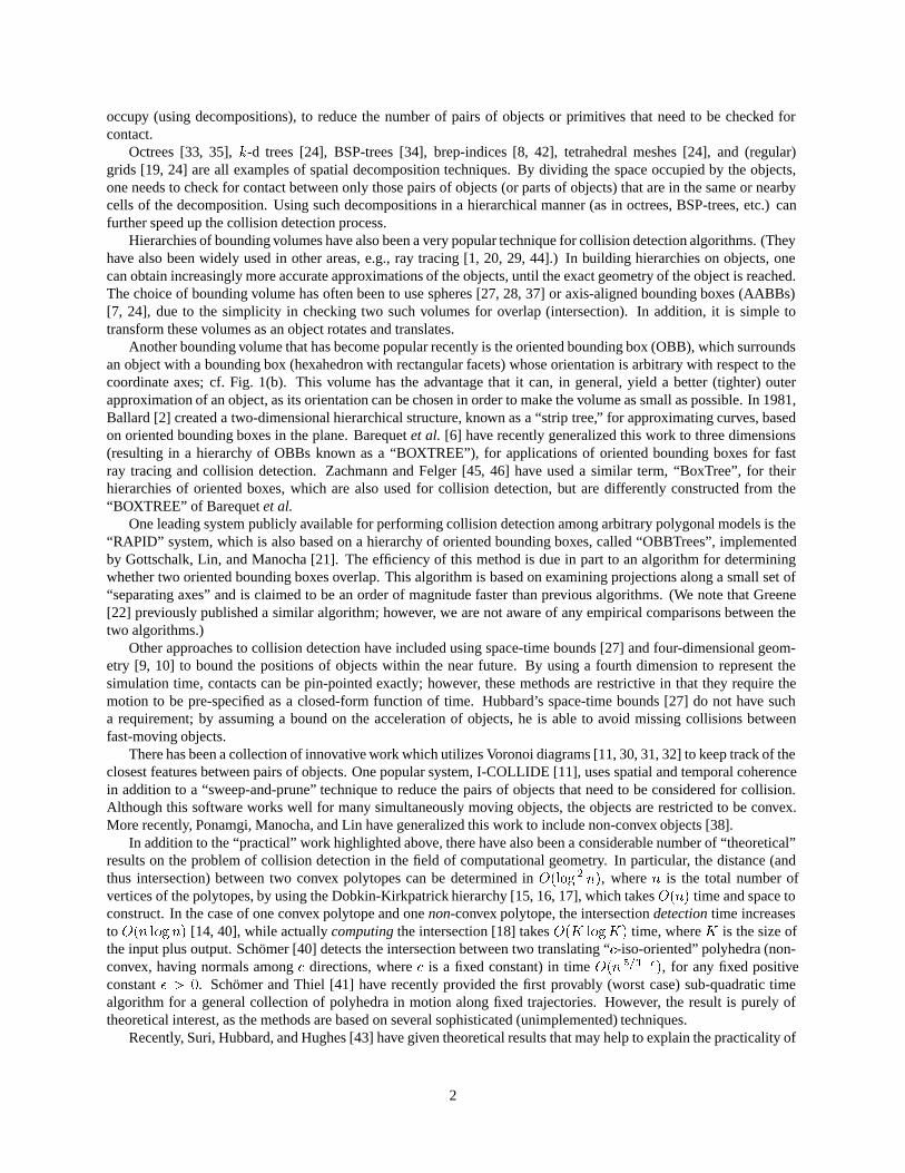
We can, however, compute worst-case upper bounds on the number of vertices in the B-rep of each of our k-dops: fork = 6; 14; 18; 26, the maximum possible number of vertices in a k-dop is 8, 24, 32, and 48, respectively.

For each node of the flying hierarchy, we store the k numbers that define a k-dop (8k bytes), two pointers to thechildren (8 bytes), the number of triangles bounded by the k-dop (4 bytes) – since the threshold is not 1 in this case,the list of triangle indices bounded by this node, the number of original B-rep vertices (4 bytes), a list of the B-repvertices, and an integer to indicate when the node was last “tumbled” (4 bytes) – to avoid re-tumbling the node if it isaccessed more than once during the CD query for one step of the flight.

In addition, we also need to store the B-rep for the convex hull associated with the root node of the flying hierarchy(Section 4.1). In the experiments reported here, the flying “Pipes” dataset required the most memory, almost 1:65megabytes, to store its convex hull.

5.1 Experimental Set-up

Our experiments have used real and simulated datasets of various complexities, ranging from tens of triangles to a fewhundred thousand triangles. We made a special effort to devise datasets that were particularly difficult for our methodand others. For instance, we considered “swept volume” datasets, in which a moving object is swept through spaceon a random motion, then numerous obstacles are randomly placed close to, but not penetrating, the swept volume;finally, we fly the object on the original path, causing it to come very close to collision with thousands of nearbyobstacles, without it actually hitting any of them. While these “challenging” datasets are unlikely to arise in practice,a goal of our study was a systematic comparison of alternative methods and alternative choices of parameters withinour own methods.

For all of the results reported here, we used a Silicon Graphics Indigo 2, with a single 195 MHz IP28/R10000processor, 192 Mbytes of main memory, and a Maximum Impact Graphics board. The code was compiled with GNUgcc (respectively, g++ for RAPID). All timings were obtained by adding the system and user times reported by the Clibrary function “times”. In order to smooth out minor variations in the timings, all tests have been run repeatedly, andwe report average times.

Although we ran RAPID on the same machine and with the same timing command, we appreciate the difficultythat exists in making comparisons between different algorithms implemented by different people. Many issues, suchas tolerances (for overlaps) and what geometric primitives to use and how they are tested for intersection, can playa crucial role in an algorithm’s performance. Also, we do not know to which extent RAPID has been optimized toachieve efficiency. (However, RAPID does use assembler code in order to speed up computations, which serves as anindication that it has certainly been optimized to some extent.)

5.2 Experimental Results

Average Costs of Cp, Cv , and Cu

We begin by reporting results of an experiment to determine the average cost of testing two primitives (triangles) forintersection, using our code. For 100,000 triangle-triangle intersection queries, all of which had their bounding boxesoverlap, in order to avoid simple rejections, the average query time per test, C p, was 0.0035 milliseconds (ms).

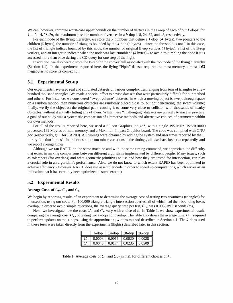
Next, we investigate how the costs Cv and Cu vary with choice of k. In Table 1, we show experimental resultscomparing the average cost, Cv , of testing two k-dops for overlap. The table also shows the average time, C u, requiredto perform updates on the k-dops, using the approximating k-dops method described in Section 4.1. The k-dops usedin these tests were taken directly from the experiments (flights) described later in this section.

6-dop 14-dop 18-dop 26-dop

Cv 0.0008 0.0016 0.0020 0.0028Cu 0.0045 0.0174 0.0235 0.0509

Table 1: Average costs of Cv and Cu (in ms), for different choices of k.

12

Average Collision Detection Query Times

Table 2 shows timing data on four typical datasets: (1) Pipes: an interweaving pipeline flying among a larger copy ofthe same system of pipes; (2) Torus: a deformed torus flying in the presence of stalagmites 12; (3) 747: a Boeing 747model flying among 25,000 random disjoint tetrahedral obstacles; and (4) Swept: an “axis-shaped” polyhedron flyingthrough a swept volume surrounded by 10,000 random tetrahedral obstacles.

In order to simulate motion of these “flying” objects, we implemented a form of “billiard paths”: a flying object ismoved along a random path, “bouncing” off of obstacles that it hits in the environment. We do not attempt to simulatea real “bounce”; rather, we simply reverse the trajectory when a collision occurs. For a more detailed look at accuratelyhandling collision response, please refer to the work by Moore and Wilhelms [33], Bouma and Vanecek [8], and thelarge collection of work by Baraff [3, 4, 5].

Timing results for a fifth dataset, Interior, are also listed in Table 2. Images of this particular flight are shown inFigures 5(a) and 5(b). This industrial dataset was provided to us by The Boeing Company and models a small sectionof the interior of an airplane. The flying object in this case is a model of a “hand”, whose path was generated by anengineer at Boeing, using a data-glove, as an example of how one would like to use collision detection when immersedon a virtual environment. Our collision detection algorithms were applied to this flight in order to detect all of thecontacts, i.e., all pairs of triangles that are in intersection, during the flight. As seen in Table 2, there were many suchcontacts for this flight, with an average of 33 contacts per step, over the 2500 steps; it was the intention of the engineergenerating the data to provide a “rigorous workout” for CD algorithms.

For comparison, we have recorded the results obtained by using the collision detection library RAPID.All of the timings reported here give the average CPU-consumption per check for collision, exclusive of rendering

and of motion simulation.

Pipes Torus 747 Swept Interior

Env. Size (no. tri.) 143,690 98,114 100,000 40,000 169,944Object Size (no. tri.) 143,690 20,000 14,646 36 404No. of Steps 2,000 2,000 10,000 1,000 2,528No. of Contacts 2,657 1,472 7,906 0 84,931

Hier. Method (ms per check)6-dop 0.487 0.294 1.639 0.582 4.37514-dop 0.392 0.191 0.760 0.153 2.70118-dop 0.366 0.184 0.356 0.109 2.75426-dop 0.525 0.210 0.415 0.076 2.639

RAPID 0.934 0.242 0.494 0.556 4.375

Table 2: Average CD Time (in ms), using our “Splatter” splitting rule.

Based solely upon these times, our 14-, 18-, and 26-dop methods perform well in comparison with RAPID’s OBBmethod, running faster on all five of the datasets; the only exception being the 14-dop method during the 747’s flight onour own generated data. As expected, the 6-dop method (i.e., axis-aligned bounding boxes), did not perform as well asthese other methods, nor as well as when using OBBs in the RAPID implementation. Out of all of our methods, usingan 18-dop for our bounding volume in the BV-trees, appears to be the best. In addition, most of the collision detectiontimes are below 2 milliseconds (many are even below 1 millisecond), which allows us to perform these queries atreal-time rates.

For the results in Table 2, all of our hierarchies were built using one of our fastest construction algorithms, basedupon the “splatter” splitting rule discussed in Section 3.3.4. We chose this algorithm because of its speed, and becauseof the fast CD query times which were obtained. As our 18-dop method appears to be the best, we have providedthe following tables which highlight the amount of preprocessing time required for all of the construction methods(longest side, min sum, min max, and splatter), as well as the CD query times which each method generated.

Table 3 highlights the amount of time (in minutes) it takes to preprocess (build) the environment hierarchy for our12Datasets 1 and 2 were graciously provided by the University of North Carolina at Chapel Hill.

13

Construction Method Pipes Torus 747 Swept Interior

Longest Side 3.61 1.61 1.69 0.31 5.78Min Sum 26.75 19.12 20.98 7.17 31.03Min Max 28.03 19.16 20.87 7.19 31.13Splatter 3.63 1.62 1.71 0.32 5.71

RAPID 1.05 0.69 0.71 0.26 1.31

Table 3: Preprocessing Time (in minutes), using our 18-dop method.

18-dop method, for each of the four construction rules: longest side, min sum, min max, and splatter 13. Our fastestmethods are clearly the “longest side” and “splatter” algorithms, which are essentially equal for all of the datasets.Likewise, the “min sum” and “min max” methods both require about the same amount of work; however, these twomethods are typically an order of magnitude slower than the others. The fastest method, in terms of preprocessing time,is RAPID, which requires only about 30-40% of the time required by the “splatter” method. The longest preprocessingtime that we have witnessed (45 minutes) occurred when using the “min max” method on the Interior dataset for the26-dop method. In order to avoid a lengthy wait each time the code is run on a standard dataset, our software has theoption to store the environment hierarchy to a binary file. For this dataset, having 169,944 input triangles, the binaryfile to store the 26-dop hierarchy is roughly 69 megabytes in size and takes just under 10 seconds to load.

Construction Method Pipes Torus 747 Swept Interior

Longest Side 0.384 0.192 0.366 0.111 3.036Min Sum 0.356 0.185 0.330 0.108 2.667Min Max 0.391 0.191 0.439 0.111 2.783Splatter 0.366 0.184 0.356 0.109 2.754

Table 4: Average CD Time (in ms), using our 18-dop method, dividing at the mean.

In conjunction with Table 3, Table 4 highlights the corresponding CD query times for each of the constructionmethods. From this table, it becomes clear that the “min sum” method is typically the best; however, unless onecan afford to spend a great deal of additional time preprocessing the environments, the best choice appears to be the“splatter” method, as it takes considerably less time to preprocess and provides CD query times that are nearly asgood.

In addition to the four construction methods that we have been mentioning, we also discussed in Section 3.3.4 theoption of splitting based on the mean versus the median of the centroid coordinates along the selected axis. In thepreceding tables, we have always used the mean. To provide some justification for our using the mean by default, wehave included Table 5, which shows the average CD query time for the 18-dop method for each of the four splittingrules when we use the median instead of the mean.

Construction Method Pipes Torus 747 Swept Interior

Longest Side 0.476 0.193 0.412 0.116 3.164Min Sum 0.450 0.192 0.359 0.111 2.822Min Max 0.530 0.196 0.450 0.114 3.080Splatter 0.481 0.194 0.396 0.113 2.774

Table 5: Average CD Time (in ms), using our 18-dop method, dividing at the median.

In comparing Tables 4 and 5, we see that using the median never results in faster query times. In quite a fewcases, the median method is at least 5% slower than the mean method, and in the “Pipes” dataset, the median method

13In each of these cases, we split at the mean rather than the median.

14

is between 24% and 35% slower for all of the entries. The preprocessing times required for the median method arealmost identical to those of the mean. In some cases it is slightly faster, in others, slightly slower.

As Tables 2– 5 report on (random) flight paths which we ourselves have generated (with the exception of theInterior flight), we have also tried to design experiments in which other methods will perform well, in order to makethis a fair comparison. In particular, the OBBTrees in RAPID are reported to perform especially well in situations inwhich there exists “parallel close proximity” between the models [21]. This situation occurs when many points on theflying object come close to several points in the environment, and a large number of the nodes of the hierarchies willhave to be searched in order to resolve all of the conflicts. Examples of this situation are in virtual prototyping andtolerance analysis applications [21]. Therefore, we have run an experiment similar to one run in [21], in order to see ifour methods based on k-dops are competitive in this situation.

We have generated datasets consisting of polygonal approximations to two concentric spheres, with the outersphere having radius 1:0, and the inner sphere being a scaled copy of the outer sphere, having radius 1:0��, for smallpositive values of �. In this “parallel close proximity” situation, all of the points of the inner sphere are very close topoints on the outer sphere, yet there is no intersection between the inner and the outer surfaces.

Here, as in [21], our objectives is to determine how many bounding volume overlap queries, N v , are required toprocess the collision detection query: Does the inner surface intersect the outer surface?

Now, as previously discussed, our default implementation uses a threshold of � = 40 to terminate the constructionof the flying hierarchies. However, RAPID uses no such threshold; it always builds a complete binary tree. Thus, inorder to make a fair comparison, we modified our code for this particular experiment to be consistent with RAPID,by using a threshold � = 1 for the flying hierarchy. Then, both methods produce trees having an identical numberof internal nodes and leaf nodes. (The structures of the hierarchies, and in particular their heights, can, of course, bedifferent.)

Hier. alphaMethod 0.55 0.1 0.055 0.01 0.0055 0.001 0.00055 0.0001

6-dop 388 49,494 76,506 109,086 113,200 116,340 116,710 116,94814-dop 32 16,888 41,782 85,656 90,896 95,150 95,564 96,05618-dop 46 11,236 34,744 79,968 86,036 91,482 92,124 92,68426-dop 22 4,652 23,774 74,052 81,160 87,622 88,322 88,968RAPID 121 3,333 7,479 41,645 60,327 91,983 95,717 100,047

Table 6: Numbers of overlap queries among k-dops of the 2,000-faceted nested spheres, for different values of alphaand k.

Hier. alphaMethod 0.55 0.1 0.055 0.01 0.0055 0.001 0.00055 0.0001

6-dop 278 289,126 494,278 1,129,398 1,223,900 1,320,158 1,329,154 1,337,11614-dop 14 85,012 239,884 831,528 960,952 1,102,260 1,115,030 1,127,90818-dop 46 55,390 194,414 762,668 903,056 1,063,346 1,079,676 1,095,86826-dop 14 12,218 119,556 675,152 831,104 1,019,272 1,038,126 1,058,072RAPID 117 2,441 5,495 43,589 87,071 428,027 609,843 932,561

Table 7: Numbers of overlap queries among k-dops of the 20,000-faceted nested spheres, for different values of alphaand k.

Tables 6 and 7 report our results for spheres of 2,000 triangles each, and spheres of 20,000 triangles each 14. Itcame as no surprise that the RAPID implementation of OBBTrees requires fewer bounding volume comparisons thanthe axis-aligned bounding boxes (6-dops). In fact, for the nested spheres of 20,000 triangles, the OBBs often requireover an order of magnitude fewer queries; this is consistent with the conclusion drawn from the similar experimentin [21].

14For these runs, we used one of our fastest construction algorithms, based on the “splatter” splitting rule.

15

Our goal here, though, was to compare the OBB method to the k-dops methods. As the tables show, for both ofthe datasets, our 14�, 18�, and 26�dop methods performed fewer bounding volume overlap queries for the largestvalue of �, 0.55, when the nested spheres are relatively well separated. For the remaining values of �, however, theOBBTrees perform considerably fewer overlap queries in the spheres dataset having 20,000 triangles. Also, OBBTreesperform fewer queries in the smaller dataset, although not by the same magnitude. Once � becomes small enough(0.001), which happens when the nested spheres are very close to one another, the k-dop methods start to overtake theOBB method.

Behavior of CD Time over Flight

While we have compiled our results primarily using the statistic of average-case collision detection time, it is importantin some applications to study the worst-case collision detection time for the flight of a moving object. On a typicalflight (that of the “Pipes” being flown within the larger system of “Pipes”), we show a plot in Fig. 3 of how the CD timevaries with position along the flight, over the 2,000 steps in the simulation. One can see that the CD time increasessubstantially at various positions along the flight; these correspond to when the flying object comes in very closeproximity to the environment. In this particular example, the maximum CD query time is roughly 18 milliseconds.

Time per Collision Detection QueryTime (ms)

Steps0.00

5.00

10.00

15.00

0 500 1000 1500 2000

Fig. 3: Individual collision detection query times for the “Pipes” dataset.

Putting an upper bound on worst-case CD time is especially important in VR applications, where one needs toperform time-critical collision detection [28]. In such situations, our algorithms can be applied, and terminated early(according to the time budgeted for each CD test), resulting in an answer of “maybe”: The flying object might beintersecting the environment at this instant. The goal, then, in using the BV-tree is to use the information present inthe search of the BV-tree, at the time of early termination, to obtain bounds on how much penetration there can be (ifat all) between the flying object and the environment. (See, e.g., [47].) This problem is left for future investigations.

6 Conclusion

We have proposed a method for efficient collision detection among polygonal models, based on a bounding volumehierarchy (BV-tree) whose bounding volumes are k-dops (discrete orientation polytopes). Our k-dops form a naturalgeneralization of axis-aligned bounding boxes, providing flexibility through the choice of the parameter k. We havestudied the problem of updating an approximate bounding k-dop for moving (rotating) objects, and we have studiedthe application of BV-trees to the collision detection problem.

Our methods have been implemented and tested, for a variety of datasets and various choices of the design pa-rameters (e.g., k). Our results show that our methods compare favorably with a leading system (“RAPID”, presentedat ACM SIGGRAPH’96 [21]), whose hierarchy is based on oriented bounding boxes. Further, our algorithms are ro-bust, relatively simple to implement, and are applicable to general sets of polygonal models. Experiments have shown

16

that our algorithms can perform at interactive rates on real and simulated data consisting of hundreds of thousands ofpolygons.

Extensions and Future Work

Throughout the paper, we have mentioned several possible extensions of our work, including some alternative methodsfor constructing BV-trees, such as

using values of k larger than 26 for our k-dops (Section 3.3.3),

using alternative “splitting rules” (Section 3.3.4), and

using a bottom-up method to construct BV-trees (Section 3.3.2).

We have also suggested some possible future investigations that could lead to faster collision detection queries, includ-ing

finding an “optimal” orientation of the initial flying hierarchy (Section 4.1),

avoiding a hard-coded threshold to control the depth of the hierarchies (Section 4.3), and

using a specially designed ordering when performing interval overlap queries (Section 4.4).

In addition to these “design” alternatives, we plan to investigate further extensions of our BV-tree methods, including:

Use of temporal coherence: From one time step to the next, the flying object will occupy roughly the same area ofour workspace and, thus, overlap roughly the same set of nodes of the environment hierarchy. It should be possibleto give our search algorithm a “hot start” at each step, thereby (potentially) greatly reducing the number of boundingvolume overlap calls. The use of coherence may also help address the problem raised at the end of the last section— that of bounding the worst-case query time, and providing an estimate of depth of possible penetration, should thequery be terminated before completion.

Multiple flying objects: Currently, our collision detection software is programmed to handle only one flying object.Incorporating multiple objects is particularly trivial if we use a brute-force approach, quadratic in the number of flyingobjects: check each flying hierarchy against the environment hierarchy, and check every pair of flying hierarchies. Ifthe number of flying objects is relatively small, this approach may be acceptable. However, if the number of flyingobjects is large, one can apply a “sweep and prune” technique, similar to the one used in [11], or possibly designeffective new strategies.

Dynamic environments: Allowing the environment to change via insertions and deletions of objects is an importantextension for work on environments that are constantly being modified, e.g., a CAD model that is under developmentand is being edited on a daily basis. The interesting research issue is that of efficiently rebalancing the BV-treehierarchies under a sequence of insertions and deletions.

Deformable objects: In addition to allowing dynamic environments, we would also like to extend our hierarchies tohandle deformable objects. By “buffering” (enlarging slightly) the k-dops in our BV-trees, we can continue to approx-imate the deformed objects over a short period of time (depending on the velocity of deformation). But rebalancingor rebuilding sections of the hierarchy will also be necessary over the course of time, and it is an interesting topic forfuture investigation to devise efficient means for doing so.

NC verification: Our methods may be applied to the task of verifying tool paths in NC (Numerically Controlled)machining, where it is important to check whether a tool penetrates (beyond a specified threshold) the surface of apart to be machined, at any position along the tool’s motion. This problem constitutes quite a challenge for a general-purpose CD code since, by the very nature of the tool motion, which is designed to sculpt the part, the tool will be inconstant contact with the part’s surface. Further, this application requires an extension of our CD code in order to beable to handle spheres and cylinders (without using polyhedral approximations), and (approximate) swept volumes.

17

Acknowledgments

Our work has greatly benefited from the support of the VR group at Boeing, including Jeff Heisserman, WilliamMcNeely, and David Mizell. We also thank Claudio Silva for valuable assistance.

Some of the datasets used during this research were provided by the University of North Carolina at Chapel Hilland Boeing Computer Services. Some datasets were also obtained from the ftp-site of Viewpoint Datalabs.

We are indebted to five anonymous referees, whose valuable comments greatly helped in the presentation andcontent of this paper.

References

[1] J. Arvo and D. Kirk. A survey of ray tracing acceleration techniques. In A.S. Glassner, editor, An Introduction toRay Tracing, pages 201–262. Academic Press, 1990. ISBN 0-12-286160-4; 3 rd printing.

[2] D.H. Ballard. Strip trees: A hierarchical representation for curves. Comm. ACM, 24(5):310-321, May 1981.

[3] D. Baraff. Curved surfaces and coherence for non-penetrating rigid body simulation. In Comput. Graphics(SIGGRAPH ’90 Proc.), volume 24, pages 19–28, Dallas, TX, USA, Aug 1990.

[4] D. Baraff. Fast contact force computation for nonpenetrating rigid bodies. In Comput. Graphics (SIGGRAPH ’94Proc.), volume 28, pages 23–34, Orlando, FL, USA, Jul 1994.

[5] D. Baraff. Interactive simulation of solid rigid bodies. Comput. Graph. Appl., 15(3):63–75, May 1995.

[6] G. Barequet, B. Chazelle, L.J. Guibas, J.S.B. Mitchell, A. Tal. BOXTREE: A Hierarchical Representation for Sur-faces in 3D. EuroGraphics’96, J. Rossignac and F. Sillion, eds., Blackwell Publishers, Eurographics Association,Volume 15, (1996), Number 3, pages C-387–C-484.

[7] N. Beckmann, H.-P. Kriegel, R. Schneider, and B. Seeger. The R �-tree: An efficient and robust access method forpoints and rectangles. In Proc. ACM SIGMOD International Conference on Management of Data, pages 322–331,1990.

[8] W. Bouma and G. Vanecek, Jr. Collision detection and analysis in a physical based simulation. In EurographicsWorkshop on Animation and Simulation, pages 191–203, Vienna, Austria, Sep 19.

[9] S. Cameron. Collision detection by four-dimensional intersection testing. IEEE Trans. Robot. Autom., 6(3):291–302, 1990.

[10] J. Canny. Collision detection for moving polyhedra. IEEE Trans. Pattern Anal. Mach. Intell., PAMI-8(2):200-209, March 1986.

[11] J.D. Cohen, M.C. Lin, D. Manocha, and M.K. Ponamgi. I-COLLIDE: An interactive and exact collision detectionsystem for large-scale environments. In Proc. ACM Interactive 3D Graphics Conf., pages 189–196, 1995.

[12] International Business Machines Corporation. User’s Guide, IBM 3D Interaction Accelerator TM , Version 1release 2.0, IBM T.J. Watson Res. Center, Yorktown Heights, NY, September 1995.

[13] A. Crosnier and J. Rossignac. T-BOX: The intersection of three mini-max boxes. Internal report, IBM T. J.Watson Res. Center, Yorktown Heights, NY, 1995

[14] D. Dobkin, J. Hershberger, D. Kirkpatrick, and S. Suri. Computing the intersection-depth of polyhedra. Algo-rithmica, 9:518–533, 1993.

[15] D. Dobkin and D. Kirkpatrick. Fast detection of polyhedral intersection. Theoret. Comput. Sci., 27:241–253,1983.

[16] D. Dobkin and D. Kirkpatrick. A linear algorithm for determining the separation of convex polyhedra. J.Algorithms, 6:381–392, 1985.

18

[17] D. Dobkin and D. Kirkpatrick. Determining the separation of preprocessed polyhedra – a unified approach. InProc. 17th Internat. Colloq. Automata Lang. Program., volume 443 of Lecture Notes in Computer Science, pages400–413. Springer-Verlag, 1990.

[18] K. Dobrindt, K. Mehlhorn, and M. Yvinec. A complete and efficient algorithm for the intersection of a generaland a convex polyhedron. In Proc. 3rd Workshop Algorithms Data Struct., volume 709 of Lecture Notes inComputer Science, pages 314–324, 1993.

[19] A. Garcia-Alonso, N. Serrano, and J. Flaquer. Solving the collision detection problem. IEEE Comput. Graph.Appl., 14:36–43, May 1994.

[20] J. Goldsmith and J. Salmon. Automatic creation of object hierarchies for ray tracing. IEEE Computer Graphicsand Applications, 7:14–20, 1987.

[21] S. Gottschalk, M.C. Lin, and D. Manocha. OBBTree: A hierarchical structure for rapid interference detection.In Comput. Graphics (SIGGRAPH ’96 Proc.), volume 30, pages 171–180, New Orleans, LA, USA, Aug 1996.

[22] N. Greene. Detecting intersection of a rectangular solid and a convex polyhedron. In P.S. Heckbert, editor,Graphics Gems IV, pages 74–82. Academic Press, 1994. ISBN 0-12-336155-9.

[23] M. Held. A library of efficient and reliable intersection routines. Technical Report, Dept. of Applied Mathematicsand Statistics, University at Stony Brook, 1997. http://www.ams.sunysb.edu/˜held/

[24] M. Held, J.T. Klosowski, and J.S.B. Mitchell. Evaluation of collision detection methods for virtual reality fly-throughs. In Proc. 7th Canad. Conf. Comput. Geom., pages 205–210, 1995.

[25] M. Held, J.T. Klosowski, and J.S.B. Mitchell. Speed Comparison of Generalized Bounding Box Hierarchies.Technical Report, Dept. of Applied Math, SUNY Stony Brook, 1995.

[26] M. Held, J.T. Klosowski, and J.S.B. Mitchell. Real-time collision detection for motion simulation within complexenvironments. In SIGGRAPH’96 Visual Proc., page 151, New Orleans, LA, USA, Aug 1996

[27] P.M. Hubbard. Collision detection for interactive graphics applications. IEEE Trans. Visual. Comput. Graph.,1(3):218–230, Sep 1995.

[28] P.M. Hubbard. Approximating polyhedra with spheres for time-critical collision detection. ACM Trans. Graph.,15(3):179–210, July 1996.

[29] T.L. Kay and J.T. Kajiya. Ray tracing complex scenes. In Comput. Graphics (SIGGRAPH ’86 Proc.), volume 20,pages 269–278, Aug 1986.

[30] M. Lin. Efficient Collision Detection for Animation and Robotics. Ph.D. thesis, Dept. Elec. Engin. Comput. Sci.,Univ. California, Berkeley, CA, 1993.

[31] M. Lin and J. Canny. Efficient algorithms for incremental distance computation. In Proc. IEEE Internat. Conf.Robot. Autom., volume 2, pages 1008–1014, 1991.

[32] M. Lin and D. Manocha. Fast interference detection between geometric models. Visual Comput., 11(10):542–561, 1995.

[33] M. Moore and J. Wilhelms. Collision detection and response for computer animation. In Comput. Graphics(SIGGRAPH ’88 Proc.), volume 22, pages 289–298, Aug 1988.

[34] B. Naylor, J.A. Amatodes, and W. Thibault. Merging BSP trees yields polyhedral set operations. In Comput.Graphics (SIGGRAPH ’90 Proc.), volume 24, pages 115–124, Dallas, TX, USA, Aug 1990.

[35] H. Noborio, S. Fukuda, and S. Arimoto. Fast interference check method using octree representation. Advancedrobotics, 3(3):193–212, 1989.

[36] J. O’Rourke. Computational Geometry in C. Cambridge University Press, New York, 1994. ISBN 0-521-44592-2.

19

[37] I. Palmer and R. Grimsdale. Collision detection for animation using sphere-trees. Comput. Graph. Forum,14(2):105–116, June 1995.

[38] M. Ponamgi, D. Manocha, and M. Lin. Incremental algorithms for collision detection between general solidmodels. In Proc. ACM Siggraph Sympos. Solid Modeling, pages 293–304, 1995.

[39] F.P. Preparata and M.I. Shamos. Computational Geometry – An Introduction. Springer-Verlag, New York, 1985.ISBN 0-387-96131-3.

[40] E. Schomer. Interaktive Montagesimulation mit Kollisionserkennung. Ph.D. thesis, Universitat des Saarlandes,Germany, 1994.

[41] E. Schomer and C. Thiel. Subquadratic algorithms for the general collision detection problem. In Abstracts ofthe 12th European Workshop on Computational Geometry (CG’96), pages 95–101, 1996.

[42] G. Vanecek, Jr. Brep-index: A Multidimensional Space Partitioning Tree. Internat. J. Comput. Geom. Appl.,1(3):243–261, 1991.

[43] S. Suri, P. M. Hubbard, and J. F. Hughes. Collision Detection in Aspect and Scale Bounded Polyhedra. Proc. 9thACM-SIAM Sympos. Discrete Algorithms, to appear, Jan 1998.

[44] H. Weghorst, G. Hooper, and D.P. Greenberg. Improved Computational Methods for Ray Tracing. ACM Trans.Graph., 3(1):52–69, Jan 1984.

[45] G. Zachmann. Exact and Fast Collision Detection. Diploma thesis, Fraunhofer Institute for Computer Graphics,Technische Hochschule Darmstadt, Fachbereich Informatik, Germany, 1994.

[46] G. Zachmann and W. Felger. The BoxTree: Enabling real-time and exact collision detection of arbitrary polyhe-dra. Proc. SIVE’95, pp. 104–113, 1995.

[47] K. Zikan and P. Konecny. Lower bound of distance in 3D. In Proc. of Winter Schoolof Computer Graphics (WSCG’97), Vol. III, pp. 640–649, 1997. Available as Technical Re-port FIMU-RS-97-01, Faculty of Informatics, Masaryk University, Czech Republic, January 1997.(http://www.fi.muni.cz/informatics/reports/)

20

(a) Level 0 (b) Level 1

(c) Level 2 (d) Level 5

Fig. 4: A spitfire aircraft, and the corresponding k-dops at different levels of the hierarchy.

21

(a) Interior (b) Close-Up

Fig. 5: A hand moving within the “Interior” dataset. The contact region is highlighted in red.

22