egun-elbt reference trajectory correction in presence...
TRANSCRIPT
EGUN-ELBT reference trajectory correction in presence ofambient fields
Dobrin Kaltchev and Kyle Gao
May 10, 2014
Abstract
The effect of ambient magnetic field on the reference trajectory (orbit) in beam-line EGUN-
ELBT is studied. We compute the deviation of central trajectory w.r.t. the vacuum chamber
axis and find the required strength of correctors or steering dipole magnets to minimize this
deviation. The final objective is to create an application tool written in either the Mathematica
language or FORTRAN, which may be useful at commissioning.
1 Introduction
Considerations are presented on the effect of residual ambient fields in the
EGUN-ELBT beam-line, a.k.a. ELBT – the E-linac injector extending from the
gun cathode to the entrance in the first cavity. The reference design [1] (TRI-
DN-10-08) assumes an ideal optics setup, focusing being provided by three short
solenoids. In [1] the electron motion in solenoid fields is modeled with Astra, [2].
In this paper, for a beam line combining solenoid fields, ambient transverse
(dipole) fields and correcting dipole magnets (steerers), we compute the reference
orbit distortion before and after its correction. The level of ambient dipole fields
for which no corrections would be needed is known to be very low – a fraction of a
Gauss. The locations of the optics elements (solenoids and dipole correctors) are
1
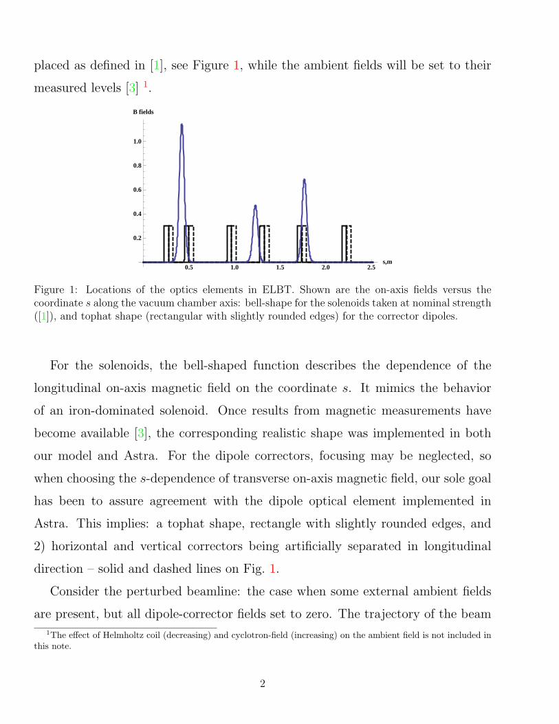
placed as defined in [1], see Figure 1, while the ambient fields will be set to their
measured levels [3] 1.
0.5 1.0 1.5 2.0 2.5s,m
0.2
0.4
0.6
0.8
1.0
B fields
Figure 1: Locations of the optics elements in ELBT. Shown are the on-axis fields versus thecoordinate s along the vacuum chamber axis: bell-shape for the solenoids taken at nominal strength([1]), and tophat shape (rectangular with slightly rounded edges) for the corrector dipoles.
For the solenoids, the bell-shaped function describes the dependence of the
longitudinal on-axis magnetic field on the coordinate s. It mimics the behavior
of an iron-dominated solenoid. Once results from magnetic measurements have
become available [3], the corresponding realistic shape was implemented in both
our model and Astra. For the dipole correctors, focusing may be neglected, so
when choosing the s-dependence of transverse on-axis magnetic field, our sole goal
has been to assure agreement with the dipole optical element implemented in
Astra. This implies: a tophat shape, rectangle with slightly rounded edges, and
2) horizontal and vertical correctors being artificially separated in longitudinal
direction – solid and dashed lines on Fig. 1.
Consider the perturbed beamline: the case when some external ambient fields
are present, but all dipole-corrector fields set to zero. The trajectory of the beam
1The effect of Helmholtz coil (decreasing) and cyclotron-field (increasing) on the ambient field is not included inthis note.
2

centroid described by the reference-particle, the one that enters at s = 0 with
kinetic energy 300 KeV and zero transverse coordinate and angle deviations, will
deviate w.r.t. the chamber axis. This is referred to as the uncorrected reference
trajectory (or orbit). The task is to find the settings for the 12 dipole correctors
that minimize this deviation. Tracking the same reference particle as above now
produces the corrected reference trajectory.
The organization of this paper is as follows.
Sect. 2 presents preliminary version of a web server that visualizes reference
orbit, beam envelopes and bunch population by tracking with Astra. An XML
format is used to describe of the EGUN-ELBT optics. The bump functions are
passed to Astra in the form of numerical tables. Users can interactively execute
Astra by choosing the entrance beam shape (assumed to be Gaussian).
Sect. 3 describes an optics code based on numerical solution of the equations of
motion (EOM) for a single electron to find the reference orbit. The code exists in
Mathematica and Fortran and, as this will be demonstrated, is in exact agreement
with Astra. To provide a bridge to optics codes, the exact EOM are first linearized
and then rewritten in Hamiltonian form (Appendix A).
Sect. 4 describes the method of optimization of dipole correctors. The math-
ematical treatment is based on the assumption that the ambient field is known.
An interleaved correction scheme is applied with increased number of correctors
involved.
In Sect. 5 we present our results on optimization of correctors for the section
extending to cavity entrance. Three cases have been tried by varying the ambient-
field region and imposed target: exact, i.e. zero orbit deviation everywhere, as
opposed to zero only at monitors:
1. a single domain of ambient field located near the cathode with exact correction
3
2. measured ambient fields with an exact correction
3. measured ambient field with correction only at the three BPM’s
Observations and conclusions are presented in Section 6.
2 Visualization of optics and beam on a web server
The ELBT optics described above and also basic characteristics of the electron
beam may be visualized on a web server:
http://beam01.triumf.ca/optdata.
Following the decision of BD group made in 2013, the server was devised as a
lattice storage tool, and should eventually provide:
• storage of E-linac sections (beam-optics lattices) in XML format;
• translation of the XML format to several of the optics codes used at Triumf:
Astra, MadX, Dimad, Optim, Transoptr and COSY Infinity;
• basic optics calculation for a lattice by remotely executing an appropriate
optics code through an Internet browser.
With regard to the ELBT, the above server allows to:
1. Display the HTML view of the optics up to the cavity exit. For example
clicking on Browse XMLs and selecting EGUN-ELBT will result in what is
shown on Figure 2.
2. Execute remotely the appropriate code. For example, click on the Select Action
button and select job "elbt-correctors" will result in Astra run of beam-
line EGUN-ELBT with correctors (steerers) installed . What happens inter-
nally is that the XML source seen on Fig. 2 is automatically parsed into an
4
input deck and then Astra executed. All input and output files are stored
in a working directory named Work Dir. Click on Refresh to check the
job status. Typical execution time is about 10 seconds. A message “all
jobs done” means that one can start browsing the working directory via
See Work Dir . Some content of sub-directory elbt-correctors is shown
on Figure 3.
3. Use Modify Astra generator to change the initial beam parameters, i.e.
particle distribution at beam-line entrance. by editing the Astra input file
generator.in. One can then repeat 2.
Figure 2 displays the XML format of optics including the cavity. and Figure 3
shows a 3D-geometry together with snapshots of the bunch at previously chosen
markers defined in the XML script (these may be monitors). For illustration, the
first corrector dipole is set at 0.5 Gs resulting in some displacement of the reference
orbit (red line). The blue lines are the one-sigma r.m.s. envelopes in transverse (x
and y) directions.
5
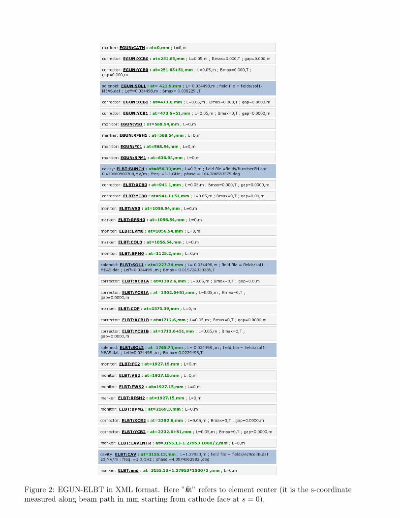
Figure 2: EGUN-ELBT in XML format. Here ”at” refers to element center (it is the s-coordinatemeasured along beam path in mm starting from cathode face at s = 0).
6
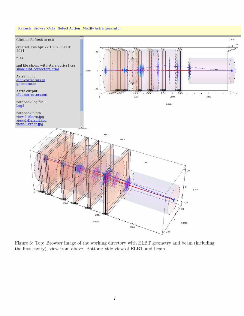
Figure 3: Top: Browser image of the working directory with ELBT geometry and beam (includingthe first cavity), view from above. Bottom: side view of ELBT and beam.
7
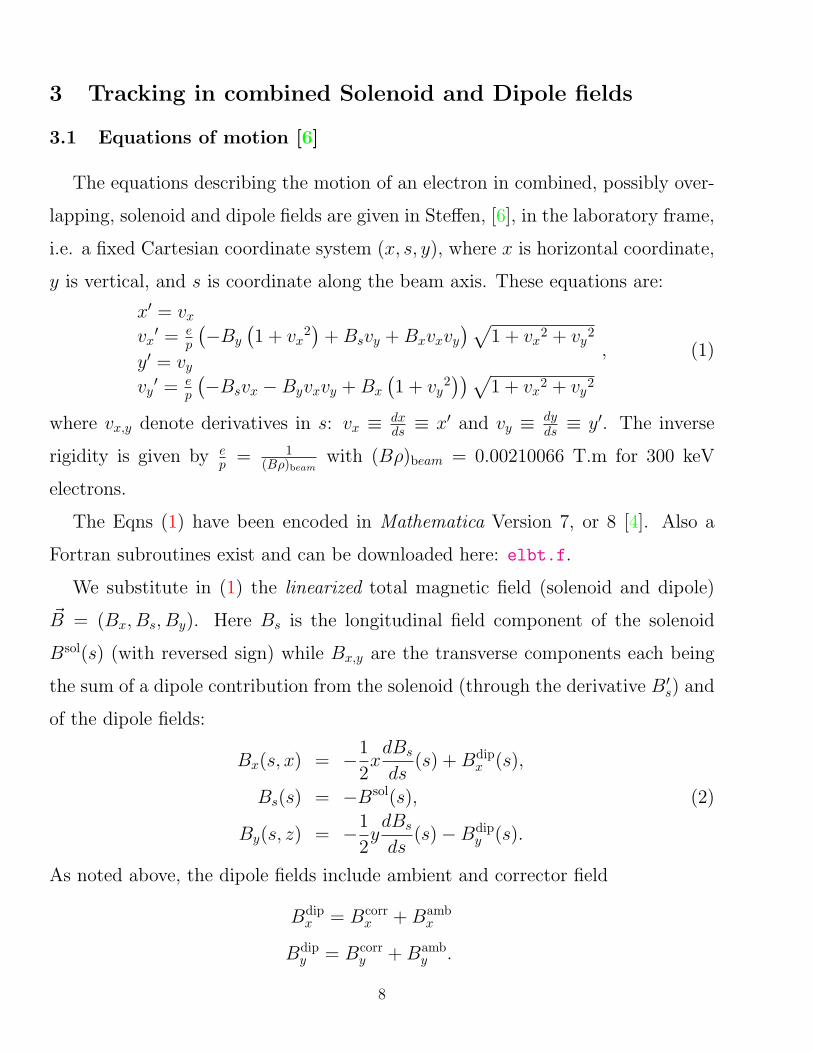
3 Tracking in combined Solenoid and Dipole fields
3.1 Equations of motion [6]
The equations describing the motion of an electron in combined, possibly over-
lapping, solenoid and dipole fields are given in Steffen, [6], in the laboratory frame,
i.e. a fixed Cartesian coordinate system (x, s, y), where x is horizontal coordinate,
y is vertical, and s is coordinate along the beam axis. These equations are:
x′ = vxvx′ = e
p
(−By
(1 + vx
2)
+Bsvy +Bxvxvy)√
1 + vx2 + vy2
y′ = vyvy′ = e
p
(−Bsvx −Byvxvy +Bx
(1 + vy
2))√
1 + vx2 + vy2
, (1)
where vx,y denote derivatives in s: vx ≡ dxds ≡ x′ and vy ≡ dy
ds ≡ y′. The inverse
rigidity is given by ep = 1
(Bρ)beamwith (Bρ)beam = 0.00210066 T.m for 300 keV
electrons.
The Eqns (1) have been encoded in Mathematica Version 7, or 8 [4]. Also a
Fortran subroutines exist and can be downloaded here: elbt.f.
We substitute in (1) the linearized total magnetic field (solenoid and dipole)
~B = (Bx, Bs, By). Here Bs is the longitudinal field component of the solenoid
Bsol(s) (with reversed sign) while Bx,y are the transverse components each being
the sum of a dipole contribution from the solenoid (through the derivative B′s) and
of the dipole fields:
Bx(s, x) = −1
2xdBs
ds(s) +Bdip
x (s),
Bs(s) = −Bsol(s), (2)
By(s, z) = −1
2ydBs
ds(s)−Bdip
y (s).
As noted above, the dipole fields include ambient and corrector field
Bdipx = Bcorr
x +Bambx
Bdipy = Bcorr
y +Bamby .
8
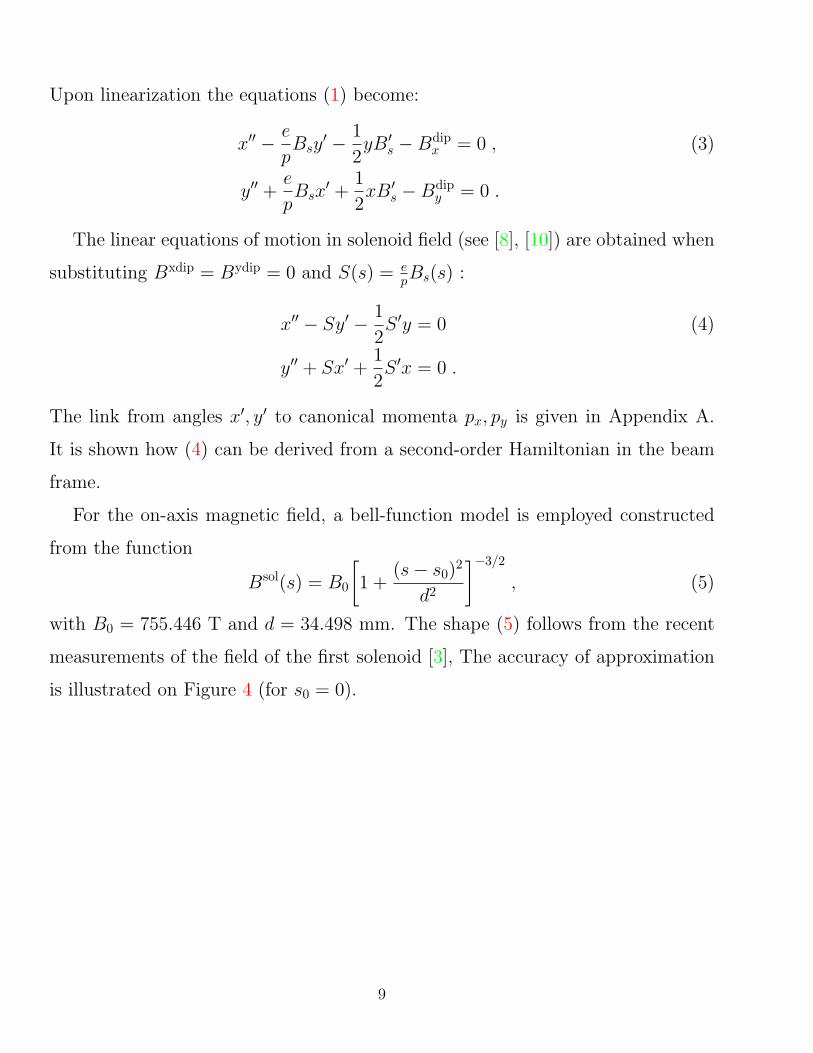
Upon linearization the equations (1) become:
x′′ − e
pBsy
′ − 1
2yB′s −Bdip
x = 0 , (3)
y′′ +e
pBsx
′ +1
2xB′s −Bdip
y = 0 .
The linear equations of motion in solenoid field (see [8], [10]) are obtained when
substituting Bxdip = Bydip = 0 and S(s) = epBs(s) :
x′′ − Sy′ − 1
2S ′y = 0 (4)
y′′ + Sx′ +1
2S ′x = 0 .
The link from angles x′, y′ to canonical momenta px, py is given in Appendix A.
It is shown how (4) can be derived from a second-order Hamiltonian in the beam
frame.
For the on-axis magnetic field, a bell-function model is employed constructed
from the function
Bsol(s) = B0
[1 +
(s− s0)2
d2
]−3/2
, (5)
with B0 = 755.446 T and d = 34.498 mm. The shape (5) follows from the recent
measurements of the field of the first solenoid [3], The accuracy of approximation
is illustrated on Figure 4 (for s0 = 0).
9
-100 -50 50 100s,mm
100
200
300
400
500
600
700
Bsol HTL
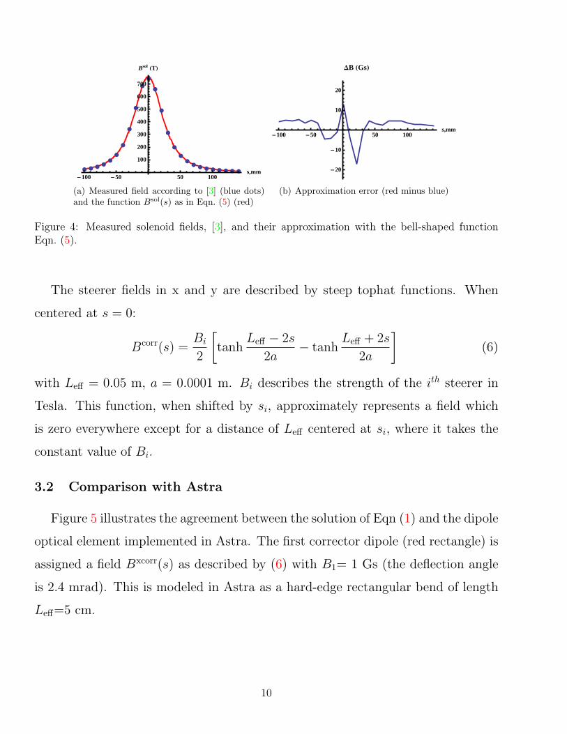
(a) Measured field according to [3] (blue dots)and the function Bsol(s) as in Eqn. (5) (red)
-100 -50 50 100s,mm
-20
-10
10
20
DB HGsL
(b) Approximation error (red minus blue)
Figure 4: Measured solenoid fields, [3], and their approximation with the bell-shaped functionEqn. (5).
The steerer fields in x and y are described by steep tophat functions. When
centered at s = 0:
Bcorr(s) =Bi
2
[tanh
Leff − 2s
2a− tanh
Leff + 2s
2a
](6)
with Leff = 0.05 m, a = 0.0001 m. Bi describes the strength of the ith steerer in
Tesla. This function, when shifted by si, approximately represents a field which
is zero everywhere except for a distance of Leff centered at si, where it takes the
constant value of Bi.
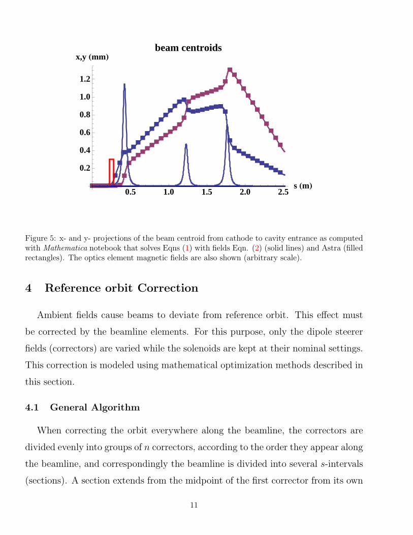
3.2 Comparison with Astra
Figure 5 illustrates the agreement between the solution of Eqn (1) and the dipole
optical element implemented in Astra. The first corrector dipole (red rectangle) is
assigned a field Bxcorr(s) as described by (6) with B1= 1 Gs (the deflection angle
is 2.4 mrad). This is modeled in Astra as a hard-edge rectangular bend of length
Leff=5 cm.
10
ààààà
à
à
ààà
àà
àà
àà
àà
ààà
ààààààààà
à
àà
àà
àà
àà
àà
à
ààààààà
à
àà
àà
àà
àà
àà
àà
à
àààààààà
à
àà
à
à
à
à
à
à
à
à
à
à
0.5 1.0 1.5 2.0 2.5s HmL
0.2
0.4
0.6
0.8
1.0
1.2
x,y HmmLbeam centroids
Figure 5: x- and y- projections of the beam centroid from cathode to cavity entrance as computedwith Mathematica notebook that solves Eqns (1) with fields Eqn. (2) (solid lines) and Astra (filledrectangles). The optics element magnetic fields are also shown (arbitrary scale).
4 Reference orbit Correction
Ambient fields cause beams to deviate from reference orbit. This effect must
be corrected by the beamline elements. For this purpose, only the dipole steerer
fields (correctors) are varied while the solenoids are kept at their nominal settings.
This correction is modeled using mathematical optimization methods described in
this section.
4.1 General Algorithm
When correcting the orbit everywhere along the beamline, the correctors are
divided evenly into groups of n correctors, according to the order they appear along
the beamline, and correspondingly the beamline is divided into several s-intervals
(sections). A section extends from the midpoint of the first corrector from its own
11
group to the midpoint of the first corrector from the next group. Starting from the
location of the first dipole, the orbit is corrected section by section in a manner of
“sliding correcting window”.
The value of n i.e. the size of the window, is gradually increased to find com-
promise between best correction and and computing time. Notice that if n =12,
all correctors are varied simultaneously to correct the orbit everywhere.
The above algorithm is easily modified for orbit correction strictly at the three
BPM’s.
4.2 Mathematica Implementation
A single electron, starting near reference orbit with initial conditions (x, y, x′, y′) =
(1µm, 1µm, 0, 0) at s = 0 is tracked. This particle experiences ambient fields and
its motion deviates from reference orbit. The orbit is then corrected using “sliding
correcting window”. Within each group or section we apply interleaved correction
scheme using Mathematica’s numerical optimization methods. The Mathematica
function FindMinimum, which locally minimizes a target function, was selected for
this task [4]. A suitable target function for orbit correction will have corrector
strengths as variables for which a minimum must exist. Furthermore that min-
imum must sufficiently optimize the orbit, that is, it must bring the generalized
coordinates ~x(s) = (x, y, x′, y′) close to the generalized reference orbit (0,0,0,0) at
requested locations along the longitudinal coordinate s.
The target function used is constructed by taking the absolute norm of the
quadratic norm of the deviations at many locations si on the beamline.
Target =N∑i=1
(4∑j=1
wjx2j(si))
1/2 (7)
Here xj’s are the components of (x, y, x′, y′). The wj’s are weight factors taken
to be 1 for angles. For positions, they are chosen to be 10 when minimizing
12
everywhere, and 3 when minimizing at BPM’s only.
When correcting the orbit only at the 3 BPM’s, then N=1 and FindMinimum
is called once for each BPM by using correctors associated with it, and si is the
location of the ith BPM.
For corrections using groups of n correctors, the si’s are defined as
si = s0 + i∆S
∆S =sn+1 − s0
N
where N is chosen to be 12, s0 is the location of the first corrector in the group in
longitudinal coordinate, and sn+1 is location of the first corrector in the next group
( or s = smax = 2.815 m for the last corrector). In this scenario, FindMinimum is
called for each group of correctors, minimizing the target function using only the
correctors in the current group.
The 12 correctors are naturally grouped into 6 pairs. This naturally splits the
beamline into 7 sections, 6 of which can be corrected (Figure 1). By choosing
group size of two, the corrected si’s matches the natural splitting of the beamline.
It was found that the target function does have a minimum which can be found
by FindMinimum for reasonable initial conditions. Furthermore, the solution opti-
mizes the orbit better than minimums of similar target functions using different
weights or p-norms.
By choosing different powers in the target function, corrections can minimize
absolute, quadratic, higher power mean, or maximum values. (Appendix B)
Furthermore, the correction is much faster when using smaller group size. De-
spite computing deviations at more coordinates, calling FindMinimum 12 times
and optimizing correctors individually is faster by a factor of 20 when compared
to optimizing the whole beamline calling FindMinimum once with all 12 correctors
at the same. However, due to how si’s are selected, different group size will result
13
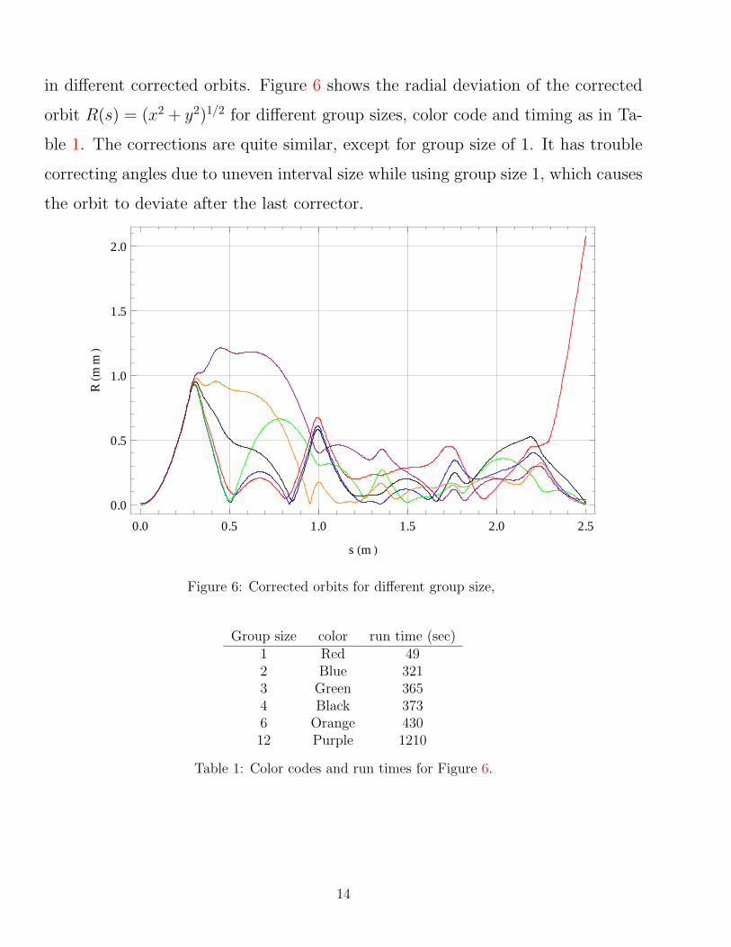
in different corrected orbits. Figure 6 shows the radial deviation of the corrected
orbit R(s) = (x2 + y2)1/2 for different group sizes, color code and timing as in Ta-
ble 1. The corrections are quite similar, except for group size of 1. It has trouble
correcting angles due to uneven interval size while using group size 1, which causes
the orbit to deviate after the last corrector.
0.0 0.5 1.0 1.5 2.0 2.5
0.0
0.5
1.0
1.5
2.0
s HmL
RHm
mL
Figure 6: Corrected orbits for different group size,
Group size color run time (sec)1 Red 492 Blue 3213 Green 3654 Black 3736 Orange 43012 Purple 1210
Table 1: Color codes and run times for Figure 6.
14
5 Results
5.1 Example of ambient field: 0.5 Gs near entrance
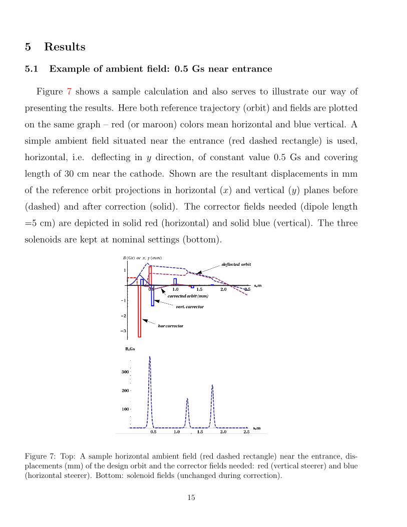
Figure 7 shows a sample calculation and also serves to illustrate our way of
presenting the results. Here both reference trajectory (orbit) and fields are plotted
on the same graph – red (or maroon) colors mean horizontal and blue vertical. A
simple ambient field situated near the entrance (red dashed rectangle) is used,
horizontal, i.e. deflecting in y direction, of constant value 0.5 Gs and covering
length of 30 cm near the cathode. Shown are the resultant displacements in mm
of the reference orbit projections in horizontal (x) and vertical (y) planes before
(dashed) and after correction (solid). The corrector fields needed (dipole length
=5 cm) are depicted in solid red (horizontal) and solid blue (vertical). The three
solenoids are kept at nominal settings (bottom).
Figure 7: Top: A sample horizontal ambient field (red dashed rectangle) near the entrance, dis-placements (mm) of the design orbit and the corrector fields needed: red (vertical steerer) and blue(horizontal steerer). Bottom: solenoid fields (unchanged during correction).
15
5.2 Measured ambient field applied everywhere with correction re-quested everywhere.
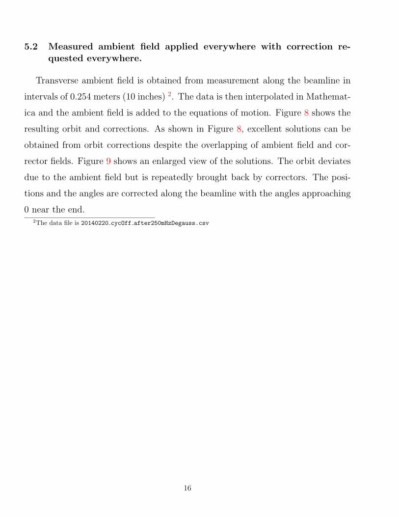
Transverse ambient field is obtained from measurement along the beamline in
intervals of 0.254 meters (10 inches) 2. The data is then interpolated in Mathemat-
ica and the ambient field is added to the equations of motion. Figure 8 shows the
resulting orbit and corrections. As shown in Figure 8, excellent solutions can be
obtained from orbit corrections despite the overlapping of ambient field and cor-
rector fields. Figure 9 shows an enlarged view of the solutions. The orbit deviates
due to the ambient field but is repeatedly brought back by correctors. The posi-
tions and the angles are corrected along the beamline with the angles approaching
0 near the end.2The data file is 20140220 cycOff after250mHzDegauss.csv
16
0.0 0.5 1.0 1.5 2.0 2.5
-20
-10
0
10
s HmL
x,y
Hmm
L
(a) Orbit before (dashed) and after (solid) correction.
0.0 0.5 1.0 1.5 2.0 2.5-0.5
-0.4
-0.3
-0.2
-0.1
s HmL
BHG
sL
(b) Ambient field everywhere.
0.0 0.5 1.0 1.5 2.0 2.50
1
2
3
4
5
s HmL
BHG
sL
(c) Corrector fields (solid).
Figure 8: Measured ambient field applied everywhere and correction requested everywhere.
17
0.0 0.5 1.0 1.5 2.0 2.5
-0.5
0.0
0.5
s HmL
x,y
Hmm
L
0.0 0.5 1.0 1.5 2.0 2.5
-4
-2
0
2
4
6
s HmL
x',y
'Hm
radL
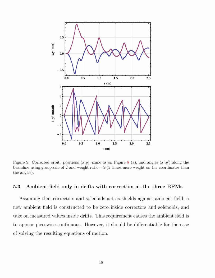
Figure 9: Corrected orbit: positions (x,y), same as on Figure 8 (a), and angles (x′,y′) along thebeamline using group size of 2 and weight ratio =5 (5 times more weight on the coordinates thanthe angles).
5.3 Ambient field only in drifts with correction at the three BPMs
Assuming that correctors and solenoids act as shields against ambient field, a
new ambient field is constructed to be zero inside correctors and solenoids, and
take on measured values inside drifts. This requirement causes the ambient field is
to appear piecewise continuous. However, it should be differentiable for the ease
of solving the resulting equations of motion.
18
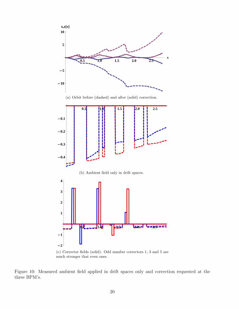
For this reason, the following ambient field was used:
Amb(s) = AmbMeasured(s)[1−N∑i=1
Bcorr(s− si)]. (8)
The measured field is multiplied by 15 inverted steerer fields (6) of height 1, shifted
up by 1. Each steerer field is centered at an si, the location of a corrector or
solenoid. This new ambient field function satisfies our requirement and its equa-
tions of motion are solvable.
Figure 10 shows the new ambient field, the resulting orbit, and its correction
at the 3 BPM’s.
19
0.5 1.0 1.5 2.0 2.5s
-10
-5
5
10
x,z@sD
(a) Orbit before (dashed) and after (solid) correction.
0.5 1.0 1.5 2.0 2.5
-0.4
-0.3
-0.2
-0.1
(b) Ambient field only in drift spaces.
0.5 1.0 1.5 2.0 2.5
-2
-1
1
2
3
4
(c) Corrector fields (solid). Odd number correctors 1, 3 and 5 aremuch stronger that even ones.
Figure 10: Measured ambient field applied in drift spaces only and correction requested at thethree BPM’s.
20
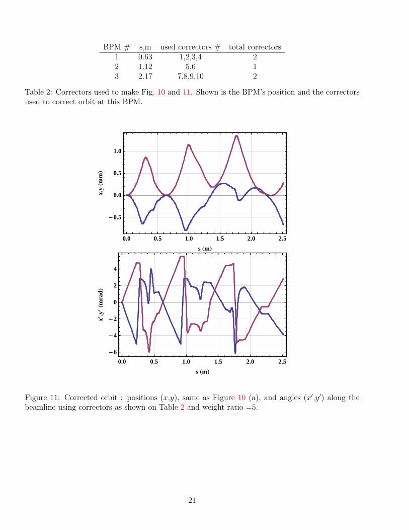
BPM # s,m used correctors # total correctors1 0.63 1,2,3,4 22 1.12 5,6 13 2.17 7,8,9,10 2
Table 2: Correctors used to make Fig. 10 and 11. Shown is the BPM’s position and the correctorsused to correct orbit at this BPM.
0.0 0.5 1.0 1.5 2.0 2.5
-0.5
0.0
0.5
1.0
s HmL
x,y
Hmm
L
0.0 0.5 1.0 1.5 2.0 2.5
-6
-4
-2
0
2
4
s HmL
x',y
'Hm
radL
Figure 11: Corrected orbit : positions (x,y), same as Figure 10 (a), and angles (x′,y′) along thebeamline using correctors as shown on Table 2 and weight ratio =5.
21

6 Summary and conclusions
We have used ambient field distribution that has a maximum of ∼ 0.5 Gs in
both planes located near entrance (Figure 8, middle). With this field the maximum
uncorrected beam-centroid deviations was larger than 2 cm, assuming the field
penetrates everywhere, and about half this value if the screening effect of the
metal envelope in solenoids and steerers is taken into account.
1. In case of ideal correction (see Figure 8): a zero deviation requested ev-
erywhere (over dense set of locations), the corrected central trajectory was
about 0.5 mm, all along the line except at the first kicker, which was also the
strongest (6 mrad), and at the entrance of the first solenoid. The trajectory
angles, or slopes. x′ and y′ at the cavity entrance can be matched to zero.
Thus near the gun the ambient field could not be efficiently corrected. The
corrector strengths are all about 3.5 - 5 Gs, except the second one, immedi-
ately after the first solenoid, which was about 2 Gs. The notebook used was
FindMin.nb
2. In the closer to the reality case (see Figure 8): with included metal-envelope
screening, but correcting only at the three BPMs, the maximum of corrected
orbit is still about ∼ 1 mm, this time distributed uniformly along the line.
Typical centroid deviations at cavity entrance were below 0.5 mm and angle
1-2 mrad. A clear corrector pattern is observed: only the odd-number 1st,3
and 5th correctors are found useful and stay at the same strengths as in 1)
above, while the even-number ones are much smaller. The notebook used was
PieceWiseFindMinBPM.nb.
. . .
22
Appendices
A Linear solenoid
The solenoid Hamiltonian, when expanded to second order: 3
H = 1/2
[(px +
S
2y)2 + (py −
S
2x)2]− p2
τ
2+
p2τ
2β2 . (9)
By defining S2 ≡ S2 , the equations of motion for the transverse coordinates are
x′ = px + S2y
p′x = (py − S2x)S2
y′ = py − S2x (10)
p′y = −(px + S2y)S2.
We now show that (10) are equivalent to (4), see Baartman [9] and Guignard, [10].
First, we solve for px in the first equation of (10) and differentiate wrt s:
p′x = x′′ − S ′2y − S2y′.
Next, we substitute p′x into equation 2 of (10)
x′′ − S ′2y − S2y′ = (py − S2x)S2.
Using equation 3 of (10), this simplifies to:
x′′ − S ′2y − S2y′ = y′S2. (11)
This can be rearranged to become the first Eqn of (4). The second Eqn of (4) is
derived in a similar manner. This proves that while the equations (10) contain no
S ′ term, the y are equivalent to (4).
3The Hamiltonian from which (9) is derived can be found in Dragt [7], where (9) is denoted by K2:
H = −√
1 + p2t − (px − Ax)2 − (py + Ay)2 − 2pt
β+
1β2− ptβ
This expression is to be expanded to second order with replaced Ax,y by S.
23
The time dependent part is of no interest as it simply produces motion in a
drift space (with τ = c(t− t0)):
τ ′ = pτ(−1 +1
β2 )
p′τ = 0 . (12)
Notice that τ ′ = pτ(βγ)2 since (−1 + 1/β2) = 1
(βγ)2 .
B Appendix Target Function
Consider the p-norm of a vector, X=(x1, ...xn), defined for p ≥ 1.
|X|p = (n∑i=1
|xi|p)1/p.
In general, a target function which must take into account the weighted contribu-
tion of deviation in canonical coordinates X=(x(s), y(s), px(s), py(s)) at different
position. This is done by taking a generalized mean of a generalized norm of X
along the beamline.
Since only the locations and not the values of extrema in the target function
are of interest, the function may be written using two p-norms:
(N∑i=1
(4∑j=1
wj|xj(si)|b)a/b)1/a.
However, the location of a local extrema of a positive target function is not shifted
after raising the function to some exponent. This can be shown by considering
an example target function T(X) positive everywhere, at a local minima T(X0).
It follows that T(X0 + δX) ≥ T(X0). Now consider taking every value of T in a
small neighborhood around X0 and raising them to some positive real number p.
Since T is always positive, we have:
T (X0) ≤ T (X0 + δX) ⇐⇒ T (X0)p ≤ T (X0 + δX)p.
24

Furthermore, minimizing |X|p, will prioritize minimizing the absolute sum of
individual xi for smaller values of p. For large values of p, it will prioritize the mini-
mizing the maximum value of x′is. http://mathworld.wolfram.com/Norm.html
By adjusting wj, a, b parameters of the previous formula, the target function
whose minimum will best correct the orbit can found.
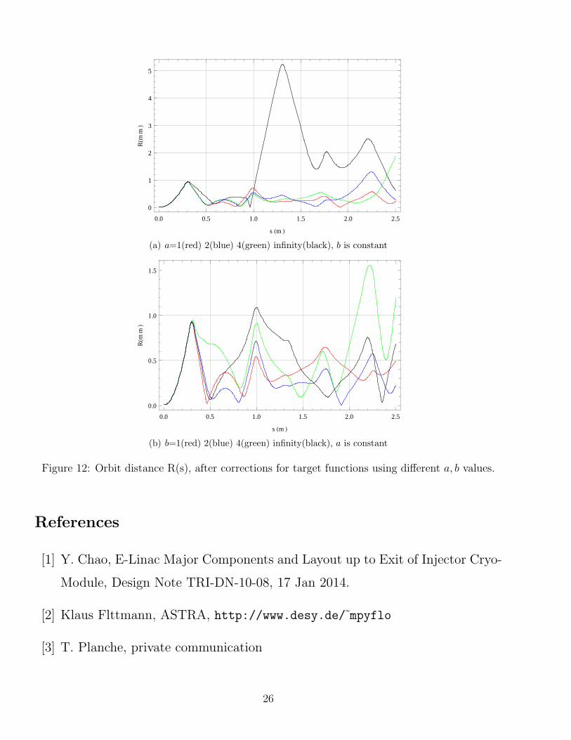
Figure 12 show that the a = 1, b = 2 make a better target function than other
attempted values, these are the values we used for orbit correction. Furthermore,
it can be seen that using a Maximum Value norm (Top: black curve, Figure 12)
may cause issues due to the discontinuities of the resulting target function.
25
0.0 0.5 1.0 1.5 2.0 2.5
0
1
2
3
4
5
s HmL
RHm
mL
(a) a=1(red) 2(blue) 4(green) infinity(black), b is constant
0.0 0.5 1.0 1.5 2.0 2.5
0.0
0.5
1.0
1.5
s HmL
RHm
mL
(b) b=1(red) 2(blue) 4(green) infinity(black), a is constant
Figure 12: Orbit distance R(s), after corrections for target functions using different a, b values.
References
[1] Y. Chao, E-Linac Major Components and Layout up to Exit of Injector Cryo-
Module, Design Note TRI-DN-10-08, 17 Jan 2014.
[2] Klaus Flttmann, ASTRA, http://www.desy.de/ mpyflo
[3] T. Planche, private communication
26
[4] Wolfram Research, Inc., Mathematica, Version 7.0, Champaign, IL (2008).
[5] B. Champion, A. Strzebonski, Wolfram Mathematica Constrained Optimiza-
tion
[6] , K. Steffen, Basic Course on Accelerator Optics, DESY, page 25 .
[7] A. J. Dragt, “Numerical Third Order Transfer Map for Solenoid”, NIM A298
(1990) 441-459
[8] G. Ripken, DESY 85-084, 1085
[9] R. Baartman, Talk at Snowmass, 2001.
[10] G. Guignard and J. Hagel, Hamiltonian treatment of betatron coupling,
CERN report
27