Eindhoven University of Technology

MASTER

Understanding the latent features of matrix factorization algorithms in movierecommender systems

Graus, M.P.

Award date:2011

DisclaimerThis document contains a student thesis (bachelor's or master's), as authored by a student at Eindhoven University of Technology. Studenttheses are made available in the TU/e repository upon obtaining the required degree. The grade received is not published on the documentas presented in the repository. The required complexity or quality of research of student theses may vary by program, and the requiredminimum study period may vary in duration.

General rightsCopyright and moral rights for the publications made accessible in the public portal are retained by the authors and/or other copyright ownersand it is a condition of accessing publications that users recognise and abide by the legal requirements associated with these rights.

• Users may download and print one copy of any publication from the public portal for the purpose of private study or research. • You may not further distribute the material or use it for any profit-making activity or commercial gain

Take down policyIf you believe that this document breaches copyright please contact us providing details, and we will remove access to the work immediatelyand investigate your claim.

Download date: 17. Jun. 2018

Eindhoven, March 25th 2011

Understanding the Latent Features ofMatrix Factorization Algorithms in

Movie Recommender Systems

byMark Graus

identity number 510562

in partial fulfilment of the requirements for the degree of

Master of Sciencein Human-Technology Interaction

Supervised by:Martijn C. WillemsenLydia MeestersZeno Gantner

TUE: School of Innovation Sciences.Series Master Theses Human-Technology Interaction (HTI)

Subject Keywords: Recommender Systems, Machine Learning, Algorithms, CollaborativeFiltering, Multidimensional Scaling, Cardsort, Multi-attribute Utility Theory, Decision Making

Abstract

Recommender systems are most often approached from a number-crunching perspective, eventhough recent algorithms are very similar to methods used in psychology. Based on these simi-larities this study tried to investigate if the prediction models produced by a matrix factorizationalgorithm can be interpreted like is done in more psychological studies. Multidimensional scalingwas used on data gathered via an online cardsort to establish the psychological attributes peopleperceive in movies. These attributes were then partially retrieved in the matrix factorizationmodel.

I

Summary

Multimedia recommender systems have been developed and improved substantially in recentyears in an attempt to help people find items relevant to their personal interests in the everincreasing amount of available content.

However, the development has traditionally been from a data-driven point of view with thegoal of predicting ratings as accurately as possible. Currently matrix factorization producesthe most accurate predictions at very low computation costs. It does so by describing moviesin terms of latent features, or dimensions underlying the rating data. Preferences can then bepredicted by using the calculated scores of the different items on these latent features.

Preferences are not only studied in the field of recommender systems. The field of decisionmaking also produced knowledge on preferences, but from a more psychological point of view.In decision making alternatives in a choice set are described on different attribute dimensions.For the choice of a notebook these dimensions might be the screen size, processor speed andamount of RAM.

The winners of the Netflix-prize suggest that the latent features in matrix factorizationsimilarly describe attributes of a movie, for example the amount to which a movie is gearedtoward men or women. The observed similarity between latent features in matrix factorizationsand attribute dimensions in decision making lead to two research questions: “What are theattributes underlying movie preferences?” and “Do the latent features in matrix factorizationdescribe these attributes?”.

If the latent features indeed describe attributes of movies, combining the knowledge ofdecision making with these latent features will provide insight in how preferences in movies areformed and provide novel user interfaces for these systems. This thesis investigates to whatextent these latent features can be interpreted.

A study was designed to investigate the relationship between the latent features and thedimensions in which people perceive movies. Using a 5-dimensional matrix factorization modela carefully constructed stimulus set consisting of 48 movies that span the model adequately wasused in an online cardsort and multidimensional scaling resulting in two attribute dimensions,‘Maturity’ and ‘Realism’. These attributes dimensions were compared to the latent featuresin the matrix factorization model. Even though the comparison demonstrated that the at-tribute dimensions and latent features are not very similar quantitatively, it turned out that atranslation from latent features into the established attribute dimensions could be found.

The translation from latent features to attribute dimensions can be used in recommendersystems to provide more user control, by allowing users to express their preferences in terms ofthese dimensions.

II

Preface

This thesis is the result of my graduation project in the group Human-Technology Interactionat Eindhoven University of Technology. It is the culmination of an education that I had thepleasure of receiving. The road that lead to this thesis has been a long and challenging one,but nonetheless one that I very much enjoyed.

As most graduate students will recognize, finishing a master thesis is not done individually.I would like to use this page to thank all those around me that took an interest in me duringmy graduation project. Apart from that I would like to thank a number of people in specific.

First of all I would like to thank my supervisors. Throughout my graduation project Martijnchallenged me to rethink my decisions in order to improve this thesis. I would like to thankLydia for the guidance she gave me, even in her free time, with performing the challenginganalyses. And lastly I would like to thank Zeno for always being ready to answer my at timesnaive questions about the algorithms. I would also like to thank all three of them for puttingup with my tight schedules and unpredictable communication.

Thanks also go out to the people that I have learned to see as my colleagues or peers:Dirk Bollen and Bart Knijnenburg. Throughout my project they were infinite sources of bothinsightful and comical input.

I would like to thank DopeLabs, manager of the radio station dubstep.fm that enabled meto keep up my energy level when needed. Related to this I would like to thank the people ofIntermate for providing me a place to drink a cup of coffee and take my mind of work whenneeded.

However, my utmost gratitude goes out to those close to me. Completing a graduationstudy is a task that demands patience and energy not only from the graduate candidate, butalso from his or her environment. I would thus like to thank my parents and my girlfriendHoi-Ying for their support and the patience they showed in face of my at times inadequatestress management. Thanks.

-Mark

Acknowledgments

Part of this work is performed under the MyMedia project1. The MyMedia project has re-ceived funding from the European Commission under the 7th Framework Programme (FP7) forResearch and Technological Development under grant agreement no. 215006.

1http://www.mymediaproject.org

IV

Contents

1 Introduction 31.1 Recommender Algorithms . . . . . . . . . . . . . . . . . . . . . . . . . . . . . . . 3

1.1.1 Content-Based . . . . . . . . . . . . . . . . . . . . . . . . . . . . . . . . . 31.1.2 Collaborative Filtering . . . . . . . . . . . . . . . . . . . . . . . . . . . . . 41.1.3 Content-Based compared to Collaborative Filtering . . . . . . . . . . . . . 41.1.4 Matrix Factorization . . . . . . . . . . . . . . . . . . . . . . . . . . . . . . 5

1.2 Evaluating algorithms . . . . . . . . . . . . . . . . . . . . . . . . . . . . . . . . . 61.3 MAUT . . . . . . . . . . . . . . . . . . . . . . . . . . . . . . . . . . . . . . . . . . 7

1.3.1 Comparing MAUT to MF . . . . . . . . . . . . . . . . . . . . . . . . . . . 81.4 Exploring the Latent Feature Space . . . . . . . . . . . . . . . . . . . . . . . . . 9

2 Layout of the Study 112.1 Multidimensional Scaling . . . . . . . . . . . . . . . . . . . . . . . . . . . . . . . 112.2 Cardsort . . . . . . . . . . . . . . . . . . . . . . . . . . . . . . . . . . . . . . . . . 122.3 Procrustes rotation . . . . . . . . . . . . . . . . . . . . . . . . . . . . . . . . . . . 122.4 Design . . . . . . . . . . . . . . . . . . . . . . . . . . . . . . . . . . . . . . . . . . 13

2.4.1 Perceived Similarity and Preference Similarity . . . . . . . . . . . . . . . . 132.4.2 Structured versus unstructured sorting . . . . . . . . . . . . . . . . . . . . 13

2.5 Summary . . . . . . . . . . . . . . . . . . . . . . . . . . . . . . . . . . . . . . . . 13

3 Movie Set 153.1 Process . . . . . . . . . . . . . . . . . . . . . . . . . . . . . . . . . . . . . . . . . 153.2 Dimensionality of the Matrix Factorization Model . . . . . . . . . . . . . . . . . 153.3 Robustness of Matrix Factorization Algorithm . . . . . . . . . . . . . . . . . . . . 16

3.3.1 Hierarchical Clustering . . . . . . . . . . . . . . . . . . . . . . . . . . . . . 193.4 Deriving Movie Set . . . . . . . . . . . . . . . . . . . . . . . . . . . . . . . . . . . 20

4 Online Study 234.1 Introduction . . . . . . . . . . . . . . . . . . . . . . . . . . . . . . . . . . . . . . . 234.2 Manipulations . . . . . . . . . . . . . . . . . . . . . . . . . . . . . . . . . . . . . . 234.3 Participants . . . . . . . . . . . . . . . . . . . . . . . . . . . . . . . . . . . . . . . 234.4 Procedure . . . . . . . . . . . . . . . . . . . . . . . . . . . . . . . . . . . . . . . . 24

5 Results 265.1 Behavioral Measures . . . . . . . . . . . . . . . . . . . . . . . . . . . . . . . . . . 265.2 Multidimensional Scaling . . . . . . . . . . . . . . . . . . . . . . . . . . . . . . . 28

5.2.1 Random Start Perceived Similarity . . . . . . . . . . . . . . . . . . . . . . 285.2.2 Remaining Conditions . . . . . . . . . . . . . . . . . . . . . . . . . . . . . 345.2.3 Comparison . . . . . . . . . . . . . . . . . . . . . . . . . . . . . . . . . . . 37

1

5.3 Conclusion . . . . . . . . . . . . . . . . . . . . . . . . . . . . . . . . . . . . . . . 40

6 Comparing Multidimensional Scaling to Matrix Factorization 426.1 Multidimensional Scaling Solution . . . . . . . . . . . . . . . . . . . . . . . . . . 426.2 Comparison to Matrix Factorization . . . . . . . . . . . . . . . . . . . . . . . . . 47

6.2.1 Inter-Movie Distances . . . . . . . . . . . . . . . . . . . . . . . . . . . . . 476.2.2 Procrustes Analysis . . . . . . . . . . . . . . . . . . . . . . . . . . . . . . 476.2.3 Clustering . . . . . . . . . . . . . . . . . . . . . . . . . . . . . . . . . . . . 486.2.4 Regressions . . . . . . . . . . . . . . . . . . . . . . . . . . . . . . . . . . . 51

6.3 Conclusion . . . . . . . . . . . . . . . . . . . . . . . . . . . . . . . . . . . . . . . 51

7 Conclusion 547.1 Perceived Similarity in Movies . . . . . . . . . . . . . . . . . . . . . . . . . . . . . 547.2 Perceived Similarity and Matrix Factorization . . . . . . . . . . . . . . . . . . . . 547.3 Issues . . . . . . . . . . . . . . . . . . . . . . . . . . . . . . . . . . . . . . . . . . 54

7.3.1 Method to Gather Similarity Data . . . . . . . . . . . . . . . . . . . . . . 557.3.2 Dimensionality . . . . . . . . . . . . . . . . . . . . . . . . . . . . . . . . . 557.3.3 Continuous Dimensions . . . . . . . . . . . . . . . . . . . . . . . . . . . . 567.3.4 Influence of Movie Set . . . . . . . . . . . . . . . . . . . . . . . . . . . . . 567.3.5 Different Sources of Data . . . . . . . . . . . . . . . . . . . . . . . . . . . 56

7.4 Conclusion . . . . . . . . . . . . . . . . . . . . . . . . . . . . . . . . . . . . . . . 57

A Matrix Factorization Models 58A.1 Procrustes Rotated Spaces . . . . . . . . . . . . . . . . . . . . . . . . . . . . . . . 58

B Multidimensional Scaling Clusters 63

References 67

2

Chapter 1

Introduction

Thanks to broadband internet the amount of movies available to any person with a connectionis virtually unlimited, while still more content is being created. This makes it increasinglydifficult for people to find movies that will match their preferences. Software systems are beingdeveloped that help users in finding content they are likely to appreciate. These systems arecalled recommender systems and are applied in a large number of domains, such as books andmovies. They are used in various applications, for example as a shopping assistant in webshopsor to provide users with personalized playlists in online music services. The study in this reportwill focus on movie recommender systems.

Current state-of-the-art recommender systems use rating information in order to make rec-ommendations. Item characteristics and user preferences are extracted from rating data anddescribed in a model (Koren, Bell, & Volinsky, 2009), an approach that overlaps with theresearch areas of decision making and preference modeling. The study in this report will in-vestigate to what extent prediction models calculated by the matrix factorization algorithmcan be interpreted. In order to do so a brief introduction into recommender system algorithmsand psychological modeling is needed, which will be provided in this first chapter. After thisintroduction a layout of the study in this report will be presented.

1.1 Recommender Algorithms

The heart of a recommender system is the recommender algorithm, or the mathematical stepsperformed to calculate what items, e.g. movies, should be recommended to the users. We candistinguish between two types of algorithms: content-based and collaborative filtering.

1.1.1 Content-Based

Content-based filtering relies on information describing the different items, like for example thecast of a movie, the director or the genre (Pazzani & Billsus, 2007). These algorithms are notused very often in movie recommenders. They are very suited in domains where the alternativescan be described in objectively measurable attributes, as for example laptop computers (wherethe attributes may be processor speed, hard disk space, internal memory etc.) or digital camera’s(number of megapixels, amount of zoom, weight etc.).

In a content-based system a user is asked to rate movies, after which the system tries topredict ratings based on the meta-information describing the movies. It is thus very similarto a regression model, with the rating as the dependent variable and the meta-information asindependent variables.

3

A content-based recommender in movies might for example use the cast of a movie, thedirector, the runtime and even the locations where the movie was shot in order to providerecommendations. If we know for one user that she gives high ratings to ‘Gangs of New York’,‘Titanic’ and ‘Catch me if you can’, it is highly likely that she likes movies starring LeonardoDiCaprio as he plays the lead role in all three movies.

1.1.2 Collaborative Filtering

Collaborative filtering algorithms rely on another type of information, namely rating informationusers express over the items. Ratings are explicit feedback on a one-dimensional scale, often ona scale from 1 to 5 stars, though there are systems that use other scales like thumbs up/thumbsdown. This rating information is combined over users to predict what items a user will like.The items with the highest predicted ratings are then presented as recommendations.

These algorithms use the similarity in rating patterns between users to base predictions on.The main rationale is that people that rate movies similarly will have a similar taste in movies.Thus if user A and user B have a similar rating pattern, the system will recommend movies touser A that user B has rated high and user A has not rated yet.

The most straightforward algorithm would be a K-nearest neighbor (KNN) algorithm. AKNN algorithm predicts the rating for an item user A has not rated yet, by taking the weightedaverage of the ratings given to this item by the K users with the most similar rating pattern touser A’s. A number of methods to improve this algorithm have been applied, by for exampletaking uncertainty of ratings into account (Jin, Si, Zhai, & Callan, 2003).

This type of algorithms can in turn be distinguished in two types of algorithms, namelymemory-based and model-based.

Memory-Based

The KNN algorithm described above is an example of a memory-based algorithm. The entiredataset is stored in memory and used when a prediction is calculated. In this case by comparingall available rating patterns and calculating an average. The problem with this approach is thatthe calculation time needed to produce predictions increases exponentially with the number ofusers and movies.

Model-Based

Another type of collaborative filtering algorithms are model-based algorithms. The most widelyused recommender algorithm is called matrix factorization and will be explained in Section 1.1.4.This type of algorithm combines rating data into a mathematical model that can be used tomake predictions. Building this model is computationally heavy and time-consuming, but cal-culating predictions in these models is done very quickly. Model-based algorithms are especiallyinteresting as we can compare the models produced by these algorithms to ways in which pref-erences are modeled in other fields of study, as we will illustrate later in this chapter.

1.1.3 Content-Based compared to Collaborative Filtering

There are advantages and disadvantages to both types of recommender approaches.The main drawback of content-based filtering compared to collaborative filtering is that it

relies heavily on the meta-data describing the items, which implies that this information shouldbe obtained and entered into the system. This also means that thought has to be put into whatmeta-data to use. Maintaining a content-based recommender system thus requires significant

4

effort, as there is a constant need to keep information up to date or to add new informationwhen new items are added to the system.

Furthermore, not all types of meta-data may be equally useful. If someone likes moviesstarring a certain actor, this can be used to make predictions. But if we consider GeorgeClooney it is hard to imagine that someone who liked him in his over the top comical role in‘Burn After Reading’ or his first role in the cult-movie ‘Attack of the Killer Tomatoes’ willautomatically like him in one of the episodes of the more serious ‘ER’.

Another issue is that not all information can be expressed easily or consistently. Somethingelementary as the genre of a movie cannot be used straightforwardly, as they are not alwaysvery well-defined (Langford, 2005; Chandler, n.d.). Users can have different interpretations ofwhat genre a movie belongs in and new genres appear or movies fall in between genres. Usinggenre information might thus pose problems when a system relies on this information. Similarto genre, it may be hard to describe movies in terms of the emotions they evoke, even thoughthis may play an important role in how someone likes a movies. One movie may evoke differentemotions in different people. And even if there would be consistency, it may be hard to describeit in words.

Collaborative filtering does not rely on this type of information, which makes it useful indomains where it is not clear what attributes of the items cause preferences. A main shortcomingof collaborative filtering algorithms however is what is called the cold start problem. Sincethese algorithms rely on rating information, it is impossible to recommend items that have notbeen rated to users, or to give recommendations to users that have not provided any ratinginformation.

Additionally, since these systems rely on rating information, it is necessary for users toshare their ratings. Users that are very conscious of their privacy may experience this needto share as an issue. In content-based recommender systems there is no need to share theinformation between users, because the models only use personal ratings and similarities interms of meta-information instead of comparing rating patterns between users.

Taking these advantages and disadvantages into consideration the conclusion is that differentapproaches are better suited for different domains. There have been attempts at combiningboth collaborative filtering and content-based filtering in movie recommenders to circumvent theshortcomings of both algorithms (Balabanovic & Shoham, 1997; Melville, Mooney, & Nagarajan,2002), but because of the ease of maintaining a collaborative filtering system, it is used asalgorithm for the majority of recommender systems nowadays.

1.1.4 Matrix Factorization

Matrix factorization is currently the most effective and efficient recommender algorithm. It issimilar to methods like Principal Component Analysis and Singular Value Decomposition inthat it tries to extract patterns embedded in data. This is done by decomposing one matrixinto two matrices, such that the inner product of these matrices reproduce the original matrix.

In the case of a recommender algorithm, it tries to describe the user-item matrixR (Table 1.1,which is an n × m matrix (with n the number of users and m the number of items in thecatalogue). The cells in R describe how the corresponding user rated the corresponding movie.R typically has a large number of missing values, as most users rate only a small amount ofmovies.

R is decomposed into two matrices, U (n × k-dimensional) and I (m × k-dimensional),such that R = U · IT . The k columns in these matrices are called the latent features. Whatthey describe exactly is unknown, but allegedly they describe attributes of movies on whichpreferences are based (Koren et al., 2009). An example might be suspense, as some people like

5

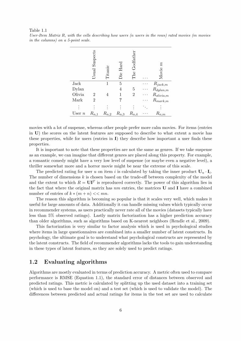
Table 1.1User-Item Matrix R, with the cells describing how users (n users in the rows) rated movies (m moviesin the columns) on a 5-point scale.

Usu

alS

usp

ects

Tit

anic

Die

Hard

Th

eG

od

fath

er

· · · Mov

iem

Jack 1 5 · · · Rjack,m

Dylan 4 5 · · · Rdylan,m

Olivia 2 4 1 2 · · · Rolivia,m

Mark 2 ? · · · Rmark,m...

......

......

. . ....

User n Rn,1 Rn,2 Rn,3 Rn,4 · · · Rn,m

movies with a lot of suspense, whereas other people prefer more calm movies. For items (entriesin U) the scores on the latent features are supposed to describe to what extent a movie hasthese properties, while for users (entries in I) they describe how important a user finds theseproperties.

It is important to note that these properties are not the same as genres. If we take suspenseas an example, we can imagine that different genres are placed along this property. For example,a romantic comedy might have a very low level of suspense (or maybe even a negative level), athriller somewhat more and a horror movie might be near the extreme of this scale.

The predicted rating for user u on item i is calculated by taking the inner product Uu · Ii.The number of dimensions k is chosen based on the trade-off between complexity of the modeland the extent to which R = UIT is reproduced correctly. The power of this algorithm lies inthe fact that where the original matrix has nm entries, the matrices U and I have a combinednumber of entries of k ∗ (m+ n) << mn.

The reason this algorithm is becoming so popular is that it scales very well, which makes ituseful for large amounts of data. Additionally it can handle missing values which typically occurin recommender systems, as users practically never rate all of the movies (datasets typically haveless than 5% observed ratings). Lastly matrix factorization has a higher prediction accuracythan older algorithms, such as algorithms based on K-nearest neighbors (Rendle et al., 2009).

This factorization is very similar to factor analysis which is used in psychological studieswhere items in large questionnaires are combined into a smaller number of latent constructs. Inpsychology, the ultimate goal is to understand what psychological constructs are represented bythe latent constructs. The field of recommender algorithms lacks the tools to gain understandingin these types of latent features, so they are solely used to predict ratings.

1.2 Evaluating algorithms

Algorithms are mostly evaluated in terms of prediction accuracy. A metric often used to compareperformance is RMSE (Equation 1.1), the standard error of distances between observed andpredicted ratings. This metric is calculated by splitting up the used dataset into a training set(which is used to base the model on) and a test set (which is used to validate the model). Thedifferences between predicted and actual ratings for items in the test set are used to calculate

6

the RMSE. Other metrics exist, but rely on the same training/testing procedure. An extensiveoverview of different metrics, their uses and differences is given in Herlocker, Konstan, Terveen,and Riedl (2004).

RMSE =

√√√√ 1

N

N∑j=1

(Ru,i −Ru,i)2 (1.1)

One of the most notable examples of this focus on accuracy was the Netflix Prize1 thatran from 2007 until 2009. Netflix is a US-based online video store that uses a recommendersystem to provide its users with recommendations of movies to watch. The goal of the contestthey organized was improving the accuracy of their recommender algorithm called Cinematchby 10%. In the end this contest was won when two teams combined their results (Koren et al.,2009).

However, some aspects of recommender system performance are claimed to be impossibleto describe by only looking at objective metrics of accuracy (McNee, Riedl, & Konstan, 2006a).This opinions is shared by a number of researchers that put effort in developing recommenderevaluation frameworks (McNee, Riedl, & Konstan, 2006b; Knijnenburg, Meesters, Marrow, &Bouwhuis, 2010).

The study in this thesis is based on the observed similarity between matrix factorizationmodels and a psychological framework used in decision making studies to describe preferences.It will adopt a psychological point of view which may lead to an understanding of what aspectsof movies are important for predicting preferences, which is useful in developing recommenderalgorithms. The psychological framework that will be used is called multi-attribute utilitytheory (MAUT) and will be explained in the next section.

1.3 MAUT

MAUT is a theoretical framework applied in decision making used to describe and explainpreferences. Its background comes from economy and assumes that a decision maker assigns asubjective value to alternatives called utility. The option in a choice set with the highest utilityis preferred over the others.

MAUT presupposes that alternatives can be described on a set of attributes. Laptops forexample can be broken down into the processor speed, weight, battery life, screen size andhard disk space (see Table 1.2). For different decision makers, different attributes can be moreimportant; one user may prefer portability over speed, while another may think screen size isthe most important attribute. Utility is a subjective value that depends on the attributes analternative has and how important a user thinks the different attributes are.

Customer A could care a lot about disk space and not so much CPU speed, while customerB cares more for processor speed and not so much disk space. When confronted with a choiceset consisting of three alternative configurations (see Table 1.2), A and B might have differentpreferences. Preferences are thus a combination between two important concepts, the userweights and the attribute values.

U(x) =K∑k=1

wkuk(xk) (1.2)

These preferences can also be calculated using Equation 1.2. This equation describes howthe individual user weights (wk) and attribute values (xk) are combined to calculate the overall

1http://www.netflixprize.com/

7

Table 1.2Alternatives with Attribute Values and User Utility Values

Attributes Utility Values

Diskspace(10 GB)

CPUspeed(GHz)

Price(100 ¤)

UserA

UserB

Alternative 1 1 0.9 3 -0.1 -0.1Alternative 2 2 0.9 5 0.4 -0.7Alternative 3 0.8 2.2 5 -0.7 0.7

utility for alternative x. The attribute values are transformed via a utility function, uk(xk),which basically describes the law of diminishing marginal returns (increasing hard disk spacefrom 10 to 20 gigabytes is appreciated more than increasing from 120 to 130) (Payne, Bettman,& Johnson, 1993).

For the sake of argument we take the utility functions to be uk(x) = x. Since this isan example, we fill in the individual user weights for the two users described in the previousparagraph. Normally these weights are derived from observed preferences, but for the sake ofillustration the weights in this example are decided to be 2 for an attribute that is important and1 for a less important attribute. If we denote the weights as w = (wdiskspace, wcpuspeed, wprice),the easiest way to describe these weights will be (2, 1,−1) for user A and (1, 2,−1) for user B(a higher price affects utility negatively, thus it is given a negative weight). The higher weightwdiskspace describes the higher importance of harddisk space for user A. Similarly, the higherweight for wcpuspeed describes the higher importance of processor speed for user B.

Using these values, we calculate the utility values as in the two right columns in Table 1.2.Through these values we can see that user A prefers Alternative 2 to Alternative 1 and Alter-native 1 to Alternative 3, whereas B prefers Alternative 3 to Alternative 1 and Alternative 1to Alternative 2, as expressed by the higher utility values for these alternatives.

1.3.1 Comparing MAUT to MF

It is worth noting that calculating the utility is almost equivalent to calculating the predictedrating in Matrix Factorization. Both the user weights (uk) and the attribute values (xk) inEquation 1.2 are similar to the latent feature scores described by Uu and Ii used to predictRu,i in matrix factorization (see Equation 1.3). A difference is that in MAUT attribute valuesare transformed via the individual attribute utility functions uk(xk). In matrix factorizationextreme latent feature scores are prevented by penalizing too high scores, which is in essencesimilar to these utility functions.

Ru,i = Uu · Ii =K∑k=1

Uu,kIi,k (1.3)

Both MAUT and matrix factorization express alternatives in a multidimensional attributespace. Furthermore, preferences are expressed as alternatives with a higher score on a one-dimensional scale (rating in matrix factorization, overall utility in MAUT).

There are two main differences between the multidimensional spaces used in MAUT andmatrix factorization. The first is the fact that dimensions in MAUT are readily interpretableas they describe the different, objectively measurable, attributes of the alternatives. In matrixfactorization the dimensions are latent features that optimally describe ratings. So even though

8

Koren et al. (2009) claim that the dimensions describe properties of the movies, there is nostraightforward way to interpret them.

Another difference is in the multidimensional structure underlying both approaches. Thedimensions in MAUT are typically correlated, as for example faster processors are more expen-sive. In matrix factorization the latent features are extracted so that they predict ratings asaccurately as possible, which will presumably lead to orthogonal latent features2. Thus wherein MAUT trade-offs have to be made between price and processor speed, in matrix factorizationa user can for example decide on various levels of comedy for a given level of suspense.

1.4 Exploring the Latent Feature Space

The key overlap between matrix factorization and MAUT lies in that both approaches assumea multidimensional space in which preferences can be represented. The meaning of the dimen-sions in MAUT is known, as these are the values of attributes of the alternatives. In matrixfactorization the meaning of the latent features is unknown, but since they are used in a similarfashion, they likely describe characteristics of items as well. By this line of thinking, we attemptto investigate what the latent features describe.

The observed resemblance between multidimensional spaces in MAUT and matrix factor-ization models gives rise to a number of research questions. The first question is concernedwith to what extent preferences or perceived similarity in movies can be described in terms ofcontinuous dimensions like is done in MAUT.

RQ1: What are the dimensions underlying perceived similarity and preferences in movies?

This question will be answered via card sorting and a method called multidimensional scal-ing, which will be discussed in the following chapter. If we can find an answer to this question,the next step is to investigate to what extent these dimensions relate to the matrix factorizationmodel space.

RQ2: Are the latent features describing a matrix factorization model similar to the dimensionsdescribing perceived similarity and preferences?

Answers to these two research questions will provide more insight in a number of areas. Theywill provide understanding in how perceived similarity in the domain of movies is structuredand to what extent this perceived similarity is captured in matrix factorization models.

Finding a positive answer to RQ1 and RQ2 can help in applying knowledge acquired inthe field of decision making on recommender systems. In studies on consumer decision makingit is already demonstrated that the composition of a choice set influences consumer satisfaction(Fasolo, Hertwig, Huber, & Ludwig, 2009). Bollen, Knijnenburg, Willemsen, and Graus (2010)demonstrated that this to some extent also applies in recommender systems.

Finding an interpretation for the dimensions in matrix factorization may help in overcominga number of problems in recommender systems. The first problem that can be overcome is thecold start problem. If the dimensions in the model space can be interpreted, a user new tothe system could express the extent to which he desires the different dimensions in movies (i.e.setting her own user vector), so that the system can recommend movies. Similarly for a newitem, users could express to what extent the movie scores on the different dimensions. Thisinformation can then be used to calculate initial vectors for users (items), so that they canreceive recommendations (be recommended) without having to rate movies (be rated).

The second problem is the influence temporary external factors may have on preferences.It has been found that emotions can influence the decisions people make (Pham, 1998), so

2An inspection demonstrated that for models under 10 dimensions the latent features are orthogonal

9

similarly a user might prefer different movies when in a different mood. The audience a moviewill be enjoyed in may similarly influence a user’s appraisal of the movie (i.e. when someone iswatching a movie by herself, she is likely to prefer different movies than when watching withother people).

In current recommender systems there is no straightforward way to take these temporaryinfluences into consideration. A way in which this is handled is by using virtual profiles toenable sets of recommendations based on different ratings. If however the research questionscan be answered, these temporary effects could be addressed by allowing users to express atemporary higher importance for a certain dimension to get recommendations more in line withthe desired movies.

10

Chapter 2

Layout of the Study

A user study was designed to find the answers to the research questions formulated in Chapter 1.Multidimensional scaling will be used to investigate what structure people use to mentallyrepresent movies. Multidimensional scaling is widely used in psychological studies to discoverwhat attributes describe perceived similarity in stimuli with ill-defined properties (Kruskal &Wish, 1978). Comparing multidimensional spaces will be done by performing a Procrustesanalysis, a method that transforms one vector space into another. This chapter will explain thedifferent methods that will be used.

2.1 Multidimensional Scaling

Multidimensional scaling is a mathematical process where similarity data is translated into aspatial configuration (Shepard, 1980; Kruskal & Wish, 1978). It is typically applied in studiesaimed at investigating how people perceive stimuli that cannot be straightforwardly expressedin terms of attributes. An example is the study of Morse code signals (Shepard, 1963), in whichthe two dimensions describing Morse code signals appeared to be code length and the amountof dashes or dots. Another example is the study on the perception of cheese by Lawless, Sheng,and Knoops (1995), in which all cheeses could be described in two dimensions: the strength ofthe taste (nutty versus milder) and the texture (smooth versus crumbly).

Multidimensional scaling requires similarity data of stimuli in order to calculate a spatialconfiguration. There are several ways to have people express similarities (Tsogo, Masson, &Bardot, 2000). One can ask a user to make pairwise comparisons, by giving her a scale torate the similarity she perceives between two items (Kruskal & Wish, 1978). Another option istriadic comparisons, where a user is asked to express which pairs are the most and least similarin a set of three items (Novello, 2009; Tsogo et al., 2000). A third option is cardsorting inwhich a user is asked to group a number of items into groups that are similar (Lawless et al.,1995). These three methods were compared by Novello (2009), who concluded that the threedifferent methods did not lead to different results in terms of consistency. The main trade-offsto consider are the resulting resolution of the similarities, the time necessary to complete thestudy, the number of participants required and the size of the stimuli set.

The models in recommender systems are typically high-dimensional. In order to establishhigh-dimensional spaces similarities between a large amount of items are needed, as the rangeof values on multiple dimensions has to be covered. This limits the use of pairwise or triadiccomparisons, as the number of comparisons required increases exponentially with the numberof items. Secondly, since matrix factorization is used to predict preferences, we are unsurewhat type of similarity it describes, if any. The ways in which similarity is gathered will bemanipulated in order to investigate what exactly is described by the matrix factorization models.

11

These manipulations imply that a high number of participants is needed. Combining the needfor a large number of participants and a large stimuli set, the method best suited is thus acardsort.

Some semantic information is necessary to be able to interpret the dimensions if the multi-dimensional scaling solution. In order to gather this data as well, participants in the study willbe asked to describe the groups they make in terms of keywords. This data can later be plottedin the multidimensional scaling solution, making the interpretation of the dimensions easier.

The multidimensional scaling solution will provide an answer to RQ1, as when no good so-lution can be found, there apparently is no multidimensional structure in which movie similaritycan be described. If a fitting solution can be found, the next step is to compare this solutionto the original matrix factorization model space in an attempt to answer RQ2.

2.2 Cardsort

In studies combining cardsorting data with multidimensional scaling, it is essential to providethe users with a set of stimuli that meets a number of requirements:

Size – The typical amount of items used in comparable multidimensional scaling studies rangesfrom 30 to 80. Among others, this number depends on the number of dimensions, as the numberof dimensions extracted from the similarity data cannot be higher than the number of items.

Diversity – The items should be selected from throughout the entire movie space, such thatthe range of values on all latent features is as high as possible. This ensures that all latentfeatures are represented in the set of movies.

Well-known – It is essential that all participants in this study sort the same movies. Thisimplies that the movies should be fairly well-known, so that the participants have no problemsin sorting them.

Clusters – The set of movies should already consist of a number of clusters, as the task ofsorting the items might otherwise be too hard for the participants of the study.

Conventional studies applying multidimensional scaling consist of a preliminary study toensure that a stimuli set meets these requirements. In our case we start from a multidimensionalstructure described by the matrix factorization model, which provides more control to establisha set meeting these requirements. Chapter 3 will provide an in-depth description of how thisset was obtained.

2.3 Procrustes rotation

After acquiring a vector space through multidimensional scaling, this vector space can be com-pared to the original matrix factorization model space, which will be done via a Procrustesanalysis. This analysis is named after the mythical Greek Damastes (who was nicknamed Pro-crustes, which translates to ‘the stretcher [who hammers out the metal]’) that offered tiredtravelers a bed, but during the night would fit his guests to the bed by stretching them or cut-ting of extremities. The method tries to find a Euclidean transformation to change one spaceinto another. The extent to which this can be done is an indication of how comparable thevector spaces are.

12

2.4 Design

There are two main uncertainties in this study. Firstly there is the question of what thematrix factorization model space actually describes. Since a matrix factorization model isbased on rating data, the resulting model space may describe something different than perceivedsimilarity. A manipulation will be incorporated in the user study to investigate this.

The second issue is that the link between a cognitive structure in which movies are repre-sented might be different from the matrix factorization model space. A manipulation will beused to see if participants perform the sorting task differently when they are provided with astructured or unstructured sorting task.

These two manipulations will yield a 2 × 2 between subjects design, which is discussed inmore detail below.

2.4.1 Perceived Similarity and Preference Similarity

Studies applying multidimensional scaling typically ask for participants to sort items based onhow similar they think two items are, which is called perceived similarity. Researchers oftenpurposely do not specify what they understand by similarity (Novello, 2009) to ensure thatparticipants are not influenced sorting in a way they expect the researcher to like.

Based on how matrix factorization works, another interpretation of similarity has beenformulated. Since the movie vectors are used to predict ratings instead of describing similarity,their proximities might represent a different kind of similarity which we will call preferencesimilarity.

The differences between preference similarity and perceived similarity can be explained byconsidering more conventional choice sets. Two cameras with the same technical specificationsbut with different colors will likely be preferred equally (unless one thinks the color of a camera isreally important), but because of the color difference, people may perceive them to be dissimilar.These cameras thus have a high preference similarity, but a lower perceived similarity.

Because it is uncertain what the proximities in the matrix factorization model represent,the differences between multidimensional scaling solutions based on both preference similarityand perceived similarity will be investigated. A priori the expectation is that solutions basedon preference similarity are more similar to the matrix factorization model, because the matrixfactorization model tries to describe preferences.

2.4.2 Structured versus unstructured sorting

The second manipulation will serve as a way to increase the probability that the gathered datawill be similar to the original matrix factorization model. This is to ensure that even when thematrix factorization model does not describe similarity as the participants perceive it, there willbe information on how the participants perceive the matrix factorization model space.

To do this some participants will be provided with a starting configuration consisting of theoriginal matrix factorization clusters, that participants can accept right away or alter if theyfeel the need to. If the data resulting from the structured sorting task is very different from theunstructured sorting task, this can be seen as an indication that the matrix factorization modelspace is very different from the underlying cognitive structure of movie similarity.

2.5 Summary

The setup of the study is illustrated in Figure 2.1. The starting point is a matrix factorizationmodel space (top right), from which a stimuli set for the user study will be derived. The

13

Figure 2.1: Layout of this study. The study starts from a matrix factorization model (represented in the top).Via a cardsort similarity data will be gathered (represented in the matrix in the bottom right), which will beused in multidimensional scaling, resulting in a solution (represented in the bottom left) that will be comparedto the original matrix factorization model.

cardsorting will result in a similarity matrix (bottom right), which will be translated into aspatial configuration via multidimensional scaling. Via the multidimensional scaling solutionRQ1 can be answered. Comparing the multidimensional scaling solution to the original matrixfactorization model provides an answer to RQ2.

The remainder of this report is as follows: The design of a suitable set of stimuli is describedin Chapter 3. The design of the study is explained in Chapter 4. The results of the user studyand the first steps toward answering RQ1 will be described in Chapter 5. An answer to RQ2will be presented in Chapter 6. The final chapter will consist of a general discussion, a criticalreview on this study and pointers for future research.

14

Chapter 3

Movie Set

3.1 Process

This chapter explains how the matrix factorization model was used to obtain a set of moviesthat fulfills the requirements formulated in the previous chapter. The process consists of threesteps. The first step is deciding upon the number of dimensions in the matrix factorizationmodel. Choosing too few dimensions will result in the model not capturing all essential movieproperties. Too many dimensions can lead to some smaller, less meaningful patterns beingcaptured, complicating or possibly preventing the interpretation of the dimensions.

After deciding on the right number of dimensions the next step is verifying that the matrixfactorization algorithm produces constant models. As this algorithm is approximating an opti-mal solution, the resulting models are not stable with every recalculation. An investigation willbe performed to verify that these differences do not result in significantly different models butthe same vector space with rotated dimensions.

The last step is reducing this model to a manageable set of movies, that adheres to therequirements formulated in the previous chapter.

3.2 Dimensionality of the Matrix Factorization Model

As mentioned before, the movie set used in the online user study will be derived from a matrixfactorization model. This model will be based on the 10M MovieLens dataset, a set consistingof 10 million ratings by 71567 users on 10681 movies. The matrix factorization model will becalculated by the MyMedia framework1.

The first step of obtaining a good set of movies is deciding on the number of dimensionsof the matrix factorization model. This will be done via visual inspection of a scree plot,similar to establishing the number of factors in factor analysis and the number of dimensions inmultidimensional scaling. A scree plot is a graphical representation of the unexplained varianceor stress as a function of the number of dimensions. Adding dimensions will always reducethe amount of unexplained variance, but at some point the amount of variance explained byevery additional dimension will diminish. This is the point where adding more dimensionsdoes not improve the model significantly anymore, presumably because from this point on theincreased performance is achieved by overfitting noise in the underlying data and not so muchby describing the data in a model.

1MyMedia is a European-funded FP7 project which is aimed at researching recommender systems, moreinformation available at http://www.mymediaproject.org

15

Figure 3.1: RMSE as a function of number of dimensions, with the model based on 10M set (blue) and, forcomparison, a model based on the 1M set (gray).

In the case of matrix factorization, we use RMSE as indicator of model fit. RMSE is a metricthat expresses the extent to which an algorithm can correctly predict ratings (see Equation 1.1).This is calculated by splitting the dataset up into two sets, one for training and one for testing.The algorithm is trained on the training set, which is then used to predict the ratings in thetest set. The difference between the predicted and actual value is squared, summed and thetotal is square rooted. The lower the RMSE, the better the model predicts.

Because RMSE is calculated by splitting up the data, a fortunate (unfortunate) split canresult in a lower (higher) RMSE than it actually is. To overcome this problem, one can performk-fold cross validation. k-fold cross validation consists of subdividing the dataset into k bins.A total of k runs is performed using these bins, where in the kth run the kth bin is used as thetesting data and the remaining bins are used as training data. The RMSE is then averaged overthese k runs. For this investigation we used a 5-fold cross validation.

Applying the scree plot method to the matrix factorization model results in the blue line inFigure 3.12. This chart shows an elbow at around 4 or 5 latent features. In order to make surethat no crucial latent features are left out, the study will use a 5-dimensional model.

3.3 Robustness of Matrix Factorization Algorithm

After deciding to work with a 5-dimensional matrix factorization algorithm, the second stepis investigating the robustness of the algorithm producing the model. Matrix factorization isa non-deterministic algorithm, which means that every time an algorithm produces a model,it may be different. It is important to verify that models produced are consistent, except forsome possible linear transformation. In order to do this, a Procrustes analysis was performedon three vector spaces described by three models. These three models were the result of threeconsecutive runs of one algorithm fed with the same data.

2Because the 1M MovieLens dataset, consisting of 1 million ratings by 6000 users on 1000 movies, is usedmore often, RMSE-values were also calculated to serve as comparison to other algorithm implementations. It isworth noting that the elbow appears at the same place. The 10M models outperform the 1M models at everynumber of dimensions. This is probably due to the larger size of the dataset. Another issue worth noting is thatthe RMSE tends to rise again after some time. This is caused by the lack of finetuning of the hyperparameters ofthe matrix factorization algorithm. One of these parameters is the regularization, which prevents the algorithmfrom using extreme values to achieve a better fit. When the dimensionality increases, the regularization shouldnormally be decreased, something omitted in this investigation. This should have no substantial effect on theconclusions, as the regularization makes a small difference on the total RMSE.

16

Figure 3.2: Example of Procrustes Rotation, where the blue triangle is rotated to fit the red triangle:Unrotated Shapes (left) and Rotated Shapes(right)

A Procrustes analysis consists out of finding a k×k matrix (A) describing a linear transfor-mation of a vector space (M) into a target matrix (Mt) via matrix multiplication (AM = Mt).When comparing n vector spaces, there are n transformation matrices that try to transformvector space Mn to the mean shape M (Ai · Mi = M, 1 ≤ i ≤ n).

Because of the vast amounts of data, it is necessary to restrict ourselves to investigating asubset of the model. In this case the data was reduced to the 1000 movies with the highestnumber of ratings. On these subsets a Procrustes analysis allowing only for reflecting, rotationand translation was performed. Reflection is when values on one dimension are inverted for allpoints, rotation is when all points are rotated around one dimension, and translation is whenall points are shifted along one dimension. In Procrustes analysis scaling is allowed too, butsince in this case the dimensions are assumed to describe characteristics of the movies, scalingthem might introduce an unwarranted emphasis on some of the dimensions in our model.

The R2-value of a Procrustes rotation describes how comparable two vector spaces are. R2

is the Pearson correlation, or the proportion of distances between movie vectors that can beexplained by the rotation. This is demonstrated in Figure 3.2. The rotation shows that thedistances between points in the plot where the blue triangle is rotated toward the red triangle(right) are smaller than those in the plot with the original triangles (left). The proportion bywhich the distances decreases by the rotation is an indication of the similarity of the two shapes.

When comparing the three matrix factorization models, they are rotated to the mean shape,described by taking the average position for every movie over the three models. The R2-valuethen represents to what extent each of the three models could be rotated back to the mean shape.For the three different models the R2-values were R2

M1= .999, R2

M2= .997 and R2

M3= .991. A

random vector space with the same density as the three vector spaces described by the modelsleads to R2

random = .083 (averaged over 25 random shapes). As taking this subset of mostrated movies might introduce a bias, the analysis was performed with a randomly selected setof movies out of the original movie space. The outcome was very similar to the analysis withthe most rated movies, with R2

M1= .999, R2

M2= .996, R2

M3= .992 and R2

random = .087Another way to investigate the shape similarity is by visually inspecting the movie space and

how far the movies are apart after rotation. In order to do this, the three models are overlayed,with the 10 most rated movies plotted for each model. This results in a plot where every moviehas 3 points, that should lie close together if the models are isomorph. For every pair of latentfeatures, these plots are added in Appendix A.1. Worth noting is that movies in different modelshave a very close distance after the Procrustes rotation, supporting the conclusion that the three

17

Figure 3.3: Comparison of Distances in Model A on X-Axis and Model B on Y-Axis for Three Models.

models are isomorph and are thus equivalent except for some straightforward transformationconsisting out of rotation and translation.

A third way to investigate the differences in shape is by looking at the distances betweenitems. If the shapes are similar, the distances between items should likewise be similar. Toinvestigate this the distances between each possible pair of movies are plotted on the horizontalaxis for one model and on the vertical axis for another model. If the models are similar, thedistances between pairs of movies should be similar as well and the points should thus lie ona line. This is displayed in Figure 3.3. The three plots show all points very close to the linex = y, which was to be expected given the high R2-values of the Procrustes rotations.

18

3.3.1 Hierarchical Clustering

Hierarchical clustering is another way to gain insight in what aspects of movies cause them toappear close to each other in the matrix factorization model. It divides one space into smallerspaces, so-called clusters. Mathematically it produces a mapping, or subdivision, of entitiesxn = x1, . . . , xn into a collection of subsets C1, . . . , Cs. These subsets are mutually exclusiveand collectively exhaustive, such that every element in xn is member of exactly one subset inC (

⋃kj=1Cj = xn).

The hierarchical clustering is calculated by performing a number of steps that result in atree. The general procedure consists of four steps. The starting point is a clustering in whichevery movie is assigned to its own cluster, after which the steps are performed until all moviesare in one cluster.

1. Clusters are gathered,

2. Proximities between clusters are calculated,

3. Clusters are grouped together based on proximity,

4. The clusters grouped together are replaced by the new cluster.

This results in a tree in which movies are placed together that are close together in the moviespace. What clusters are grouped together exactly depends on the algorithm used. For thisstudy Ward’s method has been used. Ward’s method merges clusters with the goal of creatinghigh distances between clusters, but minimizing distances within clusters. An overview ofdifferent methods is given in Murtagh (1983).

A clustering is called to be robust if it does not change much when the set of items xn

is altered slightly. Ideally a clustering should have high similarities within clusters and lowsimilarities between clusters. If this is the case, removing any item or adding noise to the itemswill not change the clustering much.

There are several ways to investigate the robustness of a clustering (Hennig, 2008). Amethod is performed via bootstrapping, in which the original set xn is clustered a large numberof times, with every clustering performed on a slightly altered version of xn. The alterationsconsist of jitter and noise. Jitter is displacing some of the items by a little bit. Noise is removinga number of randomly selected items or adding a number of random items. If these alterationsdo not have a large effect on the clustering, the clustering is considered to be robust.

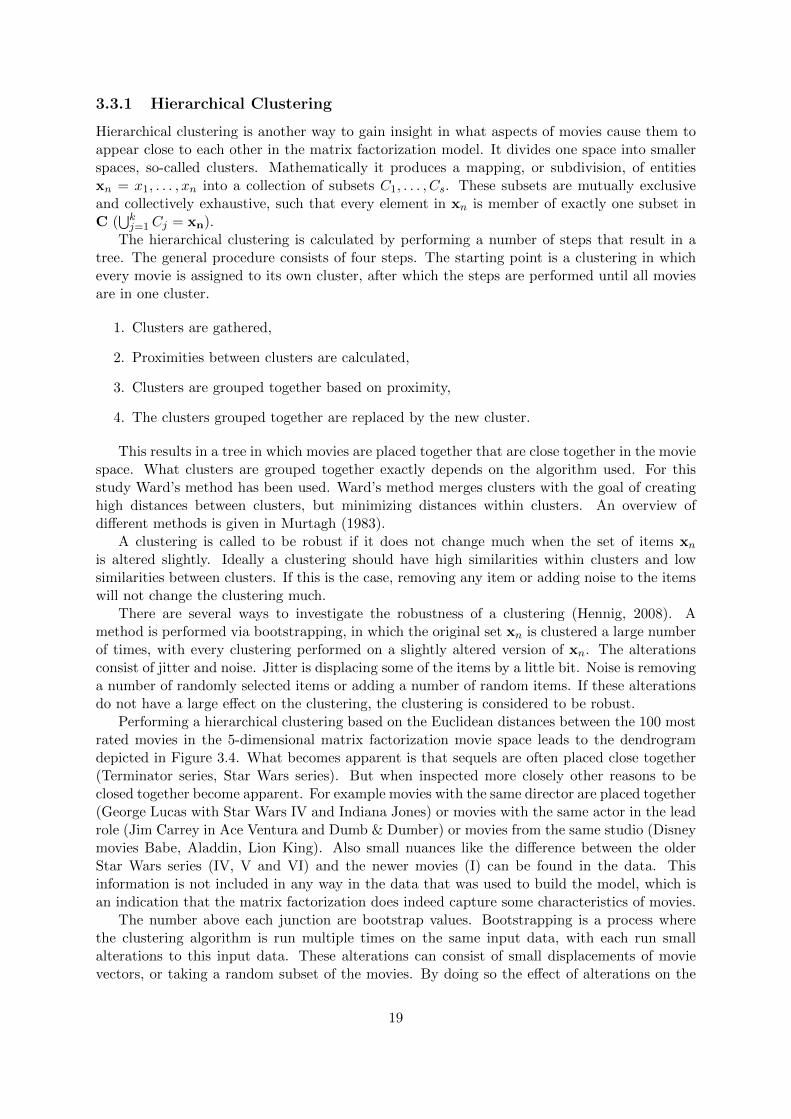
Performing a hierarchical clustering based on the Euclidean distances between the 100 mostrated movies in the 5-dimensional matrix factorization movie space leads to the dendrogramdepicted in Figure 3.4. What becomes apparent is that sequels are often placed close together(Terminator series, Star Wars series). But when inspected more closely other reasons to beclosed together become apparent. For example movies with the same director are placed together(George Lucas with Star Wars IV and Indiana Jones) or movies with the same actor in the leadrole (Jim Carrey in Ace Ventura and Dumb & Dumber) or movies from the same studio (Disneymovies Babe, Aladdin, Lion King). Also small nuances like the difference between the olderStar Wars series (IV, V and VI) and the newer movies (I) can be found in the data. Thisinformation is not included in any way in the data that was used to build the model, which isan indication that the matrix factorization does indeed capture some characteristics of movies.

The number above each junction are bootstrap values. Bootstrapping is a process wherethe clustering algorithm is run multiple times on the same input data, with each run smallalterations to this input data. These alterations can consist of small displacements of movievectors, or taking a random subset of the movies. By doing so the effect of alterations on the

19

Table 3.116 Clusters in Final Set of Movies

Cluster Movie 1 Movie 2 Movie 3

A Ace Ventura: Pet De-tective

Dumb & Dumber The Mask

B GoldenEye Mission: Impossible StargateC Jurassic Park Speed X-MenD Sleepless in Seattle Titanic While You Were Sleep-

ingE Batman Forever Home Alone WaterworldF Schindlers List The Shawshank Re-

demptionThe Usual Suspects

G The Godfather The Godfather: Part II GoodfellasH 12 Monkeys Reservoir Dogs Pulp FictionI Being John Malkovich Blade Runner FargoJ Aladdin E.T. the Extra-

TerrestrialThe Lion King

K Babe Beauty and the Beast CluelessL The Birdcage Four Weddings and a

FuneralShakespeare in Love

M Apollo 13 Dances with Wolves The FugitiveN Alien Aliens Die HardO Raiders of the Lost Ark Star Wars: Episode IV

- A New HopeStar Wars: Episode V- The Empire StrikesBack

P The Lord of the Rings:The Fellowship of theRing

The Lord of the Rings:The Two Towers

The Matrix

22

Chapter 4

Online Study

4.1 Introduction

In order to answer the research questions formulated in Chapter 1, a user study will be per-formed. The main goal of this user study is to gather information on how users perceivesimilarity between movies. These similarities will be processed using multidimensional scaling,resulting in a spatial configuration of which the dimensions will be interpreted. This spatialconfiguration will then be compared to the original matrix factorization space.

4.2 Manipulations

In Chapter 2 two manipulations were proposed to investigate what the matrix factorizationspace actually represents. These two manipulations have been operationalized in the user studyand result in a 2 × 2 between subjects design. The first manipulation is the instruction thatparticipants will receive to base their sorting on. For the two conditions the instructions wereas follows:

Perceived Similarity – ‘sort into groups of movies that you find similar’.Preference Similarity – ‘sort into group such that when movies are grouped together,

someone that likes one of the movies will like the other movies as well’.The second manipulation affected the starting configuration for the card sorting task: Half of

the participants started with a random configuration (Random condition), while the other halfstarted with the clusters as they were extracted from the matrix factorization model (Presortedcondition).

4.3 Participants

Participants were gathered via a database maintained by the university. 122 participants visitedthe online study, out of which 89 participants completed it. One of the participants finished theentire study within the unrealistic time of 3 minutes. After removing this subject a total of 43female and 45 male participants remained. The mean age was 27.2 years (SD: 8.9 years).

The participants were not equally distributed over the conditions (see Table 4.1), caused bya number of people stopping during the study, rendering their data useless.

Participants most often quit the Presorted Perceived Similarity condition. The data providesno explanation why more participants in this condition did so. A Chi Square showed that therewas no significant difference in the number of participants quiting over conditions (χ2(1, N =

23

Table 4.1Number of Participants per Condition

Starting ConfigurationPresorted Random Total

SimilarityPerceived 16 24 40

Preference 28 20 48Total 44 44 88

88) = 2.24, p = .13), but the lower participant count for the Presorted Perceived Similaritycondition has to be taken into account during the analysis.

Because the majority of participants in this database speak Dutch as first language, thestudy was conducted in Dutch.

Participant expertise was measured by three questionnaire items adopted from Bollen et al.(2010), rated on a 5-point Likert scale1. It showed no significant difference over conditions.

4.4 Procedure

The user study consisted of three parts. The first part served as general introduction to thestudy and a small survey to establish demographics on movie expertise. The second part was apractice card sorting task for the participants to get familiar with the interface. The practicetask consisted of sorting 8 cards depicting either fruits or vegetables into two piles. Participantswere instructed to make one pile for fruits and one pile for vegetables.

After the example task the users were presented with the instructions of the actual sort-ing task. These instructions emphasized that there was no single correct solution like in theexample task. Additionally the first manipulation was operationalized in these instructions,by explaining participants the type of similarity they were supposed to base their sorting on.These instructions remained visible during the actual task.

The user interface of the actual card sorting task is shown in Figure 4.1. Cards that are sortedtogether received a border with the same color. Participants were able to see the synopsis andmovie cover by pressing the button denoted ‘meer info’ (more information). When inspectingthis additional information people also had access to a button denoting ‘onbekend’ (unknown)to remove the movie from the task, if they did not know the movie. Unsorted movies had grayborders. The task instructions were presented in the top right, along with the button to confirmthat the user is ready. The top left showed a button that could be used to reset the sorting.

The cardsorting was an unstructured card sorting, that allowed people to decide on thenumber of groups themselves, as long as there were at least two groups and every card wasassigned to a group.

The second manipulation was operationalized in the starting configuration. Participants inthe Presorted conditions started out with the original clusters as they were found in the matrixfactorization, with the remark that they could either alter or accept the starting configuration.People in the Random conditions were asked whether they preferred to start with the itemsspread out, or all movies stacked in one pile. They were asked to make this decision based onhow they experienced the example task.

When finished with the sorting, people were asked to describe (tag) the groups they madein a couple of keywords. The instruction to tag the movies was deliberately postponed to after

1The three items were: “I am a movie lover”, “Compared to those around me I am a movie expert” and“Compared to those around me I watch a lot of movies”. All three were rated on a 5-point Likert scale rangingfrom ‘Disagree’ to ‘Agree’.

24

Figure 4.1: Card Sorting User Interface

the sorting task, as the knowledge of having to tag might have influenced the way participantssort.

As final step they were presented with the groups they made, and per group were askedto express how confident they were of the movies belonging together in a group and how fa-miliar they were with the movies in the group. This was expressed on a 5-point Likert scale.Additionally they were given the opportunity to elaborate on why they grouped the moviestogether.

The study took on average 15.53 minutes (SD: 6.9 minutes) to complete. For calculatingthe average, data on duration from three participants was ignored as they took longer than 60minutes to complete the entire survey. This is presumably because they got interrupted duringtheir participation. As inspecting the data did not provide any reasons to discard their data, itwill be used in further analysis.

25

Chapter 5

Results

Prior to the actual multidimensional scaling a number of behavioral measures will be investi-gated to verify the reliability of the data. A number of issues were encountered when inspectingthese behavioral measures. Five users did not provide any tags for the groups they made. Thereis no indication that they did not put serious effort into the cardsorting task, they might havesimply overlooked the tagging instructions, possibly because the participants were only askedto tag the groups after they indicated they finished sorting. Data of these participants will beignored when looking at the tags and tagging frequencies.

One user ignored the button that allowed for the removal of unknown items and created agroup tagged ‘unknown’. Movies in this group of this user will be considered as if the user diddiscard them via the button for the remainder of the study.

5.1 Behavioral Measures

Taking these issues into consideration, the average values and standard errors for the behavioralmeasures that were logged during the study are displayed in Table 5.1. Differences in these mea-sures over conditions would indicate that the participants performed the task differently whichmight lead to differences in the solutions that should be taken into account when comparingthese solutions to the original matrix factorization model.

To start, a 2-way ANOVA was performed with the duration of the sorting task as dependentvariable and the type of instruction and starting configuration as independent variables. Nosignificant effects were found, which indicates that participants spent about an equal amountof time. A significant difference would indicate that participants in some conditions spent moreor less time on the same task, which might affect the reliability of the following analyses.

A similar ANOVA was performed with the number of moves people needed to finish thetask as dependent variable. Moves consist of moving a movie to a new group or discarding amovie during the sorting task. The only marginally significant effect was the main effect ofstarting configuration (F1,84 = 3.07, p = .08). Participants in the random starting conditionperformed on average more steps (Mrandom = 46.3, SD = 27.9) than those who were given astarting configuration (Mpresorted = 36.2, SD = 25.6).

It is worth noting that these two ANOVA’s show that while less moves were needed inthe presorted start configuration, the same amount of time was required to finish the task.An explanation could be that the task consists of two subtasks. Firstly the items have tobe identified and secondly they have to be moved to the proper position. Participants in thepresorted condition can save time by not having to move items into a configuration, but theystill have to identify the movies and check the configuration. The difference in time saved by not

26

Table 5.1Mean Values and Standard Errors of Behavioral Measures per Condition

Condition N Duration Moves Number ofTags

Number ofGroups

Certainty

Start Conf. Similarity

Presorted Perceived 16 9.5 (1.7) 34.3 (4.1) 14.5 (1.3) 10.5 (0.7) 4.0 (0.2)Presorted Preference 28 8.1 (0.8) 37.4 (5.6) 14.3 (1.2) 10.0 (0.6) 3.7 (0.1)Random Perceived 24 9.0 (1.0) 48.6 (6.7) 10.4 (0.6) 7.9 (0.5) 4.0 (0.1)Random Preference 20 9.6 (1.1) 43.6 (4.7) 13.4 (1.1) 8.5 (0.5) 3.8 (0.1)

having to alter the configuration too much does not significantly reduce the total time neededto complete the sorting task.

An ANOVA with the number of groups as dependent variable was performed as well. Thefact that the presorted configuration already has a high amount of 16 groups, lead to theexpectation that people in the random start configuration would make less groups. The datashowed that the starting configuration indeed had a significant effect on the number of groupsparticipants ended with (F1,84 = 12.49, p < .001). Participants that were provided with apresorted starting configuration ended up with more groups (Mpresorted = 10.2, SD = 3.1) thandid participants who started from a random configuration (Mrandom = 8.1, SD = 2.3).

An important part of the task consisted of tagging the movies. An ANOVA on the numberof tags per group was performed. Because of the higher number of groups participants made inthe presorted conditions, the total number of tags would be expected to be higher as well. Nosignificant effects were found in the number of tags used, which indicates that people did notexperience more or less difficulties when explaining the groups they made over conditions.

One last measure to be investigated is how certain people were of the groups they made.After the sorting and tagging people were asked for every group to express how certain they werethe movies in it belonged together on a Likert scale ranging from 1 (a little certain) to 5 (verycertain). A marginally significant effect in the average certainty was caused by the instructionpeople received (F1,84 = 2.97, p = .085). People who were instructed to base their sorting onperceived similarity expressed higher certainty on their grouping (Mperceived = 4.0, SD = 0.6)than people who were instructed to base their sorting on preference similarity (Mpreference = 3.7,SD = 0.7). This indicates that the instructions caused people to approach the task differently.

One participant was noticed during the analysis because of a very low task duration and alow number of groups. This user finished the task in under three minutes and made only threeseparate groups, while the average duration was 8.9 minutes (SD: 5.1) minutes and the averagenumber of groups was 9.2 (SD: 2.9). While neither number is more than 3SD from the mean,the combination of these two low numbers lead to this participant being removed from the datafor the remainder of the study.

In summary, these investigations showed that participants went through the survey in com-parable ways. The time participants spent, the number of groups they made and the numberof tags they gave are similar when compared quantitatively, which indicates that the manipula-tions did not strongly influence how people approached their tasks. The following analyses willinvestigate if the manipulations influenced the sorting in a qualitative way.

Reliability

An additional issue to take into consideration is the reliability of the groupings. Two differentmeasures of reliability can be extracted from the data that was logged, namely the number of

27

times the movies was discarded during the card sorting task and the familiarity with the moviesin each group as expressed in the questionnaire after the card sorting task.

Based on these two measures, two movies have been removed from the data for the remainderof the analysis. These movies are ‘Fargo’ (discarded by half of the participants) and ‘theBirdcage’ (this movie was in groups for which expressed familiarity was more than 3 SD belowaverage), which leaves 46 movies for the remainder of the analysis.

5.2 Multidimensional Scaling

The similarity data gathered from the user study consists out of movies that are either groupedtogether or not, which is ordinal data. It is thus unknown how much more similar movies areif they are grouped together.

Each proximity is a value that depends on two movies and the participant. This type ofdata is what is called two-mode, three-way similarity data (Cox & Cox, 2000). Two-modeimplies that there are multiple participants and multiple stimuli. Three-way implies that everysimilarity is defined by a movie, another movie and a participant.

There are two possible approaches to use this type of data. Firstly the proximities can beaggregated over items, leading to a single frequency table expressing how often each pair ofmovies was grouped together. Secondly it is possible to use methods that take individual differ-ences into account. This study will use this second approach via the method called INDSCAL(Carroll & Chang, 1970).

INDSCAL is a non-metric multidimensional scaling method. Non-metric means that thedissimilarities are not considered to be continuous measures, but transformed using a non-linear but monotonically increasing function optimally describing the proximities. Because theproximities are not continuous anymore the absolute distances do not carry much meaning andrelative distances should be considered instead.

INDSCAL produces solutions consisting of a stimuli space and a subject space. The stimulispace describes the scores of the stimuli on the different dimensions, while the subject spacedescribes for every individual how important each dimension is in how she judges similarity.

A normal approach in multidimensional scaling starts by comparing the model fit againstthe number of dimensions and picking a dimensionality where model fit does not increase muchwhen increasing the dimensionality. This is done by visually inspecting a scree plot, with themodel fit as a function of the dimensionality, and finding the ‘elbow’ of this plot. An INDSCALsolution requires at least two dimensions to be able to describe the individual differences, whichproduces difficulties to make this plot, as the difference between one, two and three dimensionscannot be compared. Thus a possible ‘sweet spot’ at two dimensions cannot be seen in the plot.The approach that will be taken in this case is starting from the least complex 2-dimensionalsolution and investigating to what extent increasing dimensionality improves the model.

5.2.1 Random Start Perceived Similarity

The data of participants who were instructed to base their sorting on perceived similarity andstarted with a random configuration will be used as starting point for the analysis. Individualsimilarity matrices were created for the 24 subjects in this dataset. The cells in the matrixwere coded into one of three levels: 1 for pairs of movies grouped together, 0 for pairs of moviesgrouped in different groups and missing values for pairs from which one or both movies werediscarded. The resulting ordinal data was used in the SPSS implementation of INDSCAL.

Multidimensional scaling cannot handle data with a high number of equal proximities. Toovercome this problem the SPSS implementation of INDSCAL has an option called ‘Untying of

28

ties’, which alters equal values proximities in an optimal fashion.INDSCAL was run on the data of the participants, resulting in a 2-dimensional solution

with an S-Stress of 0.104. The solution was plotted to be investigated visually (see upper halfof Figure 5.1). In order to facilitate the interpretation of the solution, the tags used to describethe groups were linked to the movies in the groups. This resulted in frequencies describinghow often each movie was tagged with a certain tag. For the 10 most frequently used tagslinear regressions were performed with the dimension values of movies as predictor and the tagfrequency as dependent variable. The regression coefficients were used to draw an arrow inthe direction in which the frequency a given tag was used increased maximally (lower half ofFigure 5.1). The length of the arrows is scaled by the R2-value of the regression models. Basedon the tags a cautious interpretation may be ‘Realism’ for dimensions 1 (with ‘scifi’/‘fantasy’on one end of the dimension ‘drama’/‘romance’ on the other) and ‘Maturity’ for dimension 2(going from ‘children’s’/‘family’ to ‘action’).

Apart from the stimuli configuration, an INDSCAL solution also consists of a subject space,describing how the subjects weigh the dimensions in the multidimensional scaling when ex-pressing similarity. The subject space for this solution is displayed in Figure 5.2. The ratio ofrelative importance of the two dimensions is called ‘weirdness’ and is calculated to be higherif one dimension is more important than the other. The figure shows that while some partici-pants mainly use the first dimension how they perceive similarity, most participants use bothdimensions to at least some extent.

The next step was investigating if adding an extra dimension to the solution would improvethe solution. Displaying the three-dimensional solution is harder to do, but a representation ofthe configuration is displayed in Figure 5.3 (S-Stress: 0.083). To increase the understandabilityof this plot, the movies in the solution space have been clustered using Ward’s hierarchicalclustering as was done in Hollins, Faldowski, Rao, and Young (1993). Items in the differentclusters are interconnected by lines. To have a readable figure only one movie title for eachcluster is shown. Table B.1 in Appendix B shows what movies were in each cluster.

The most noteworthy observation is that where the tag vectors formed a cross in the twodimensional solution, they form a tetrahedron in three dimensions. A tetrahedron is a shape thatis formed by joining four equilateral triangles along the edges (i.e. a pyramid with a triangularbasis instead of the more common square basis). In this case the origin of the solution is inthe center of this shape, with the tags pointing into the corners of the tetrahedron, which isillustrated in Figure 5.4.

The ‘action’ tag points down and out of the page into one corner, the ‘romantic’ and ‘drama’tags both point into the corner in the page and to the right, the ‘scifi’ and ‘fantasy’ tags pointin the third corner going in the page and to the left and the ‘children’ and ‘family’ point upinto the last corner. ‘Quality’ does not point into any of the corners, but is halfway between‘romantic’/‘drama’ and ‘action’. Similarly ‘comedy’ is halfway between ‘romantic’/‘drama’ and‘children/family’.

Much like the cross encountered in the 2-dimensional solution, the tetrahedron is a shape inwhich the tags are separated from each other as much as possible. This might be an indicationthat the movies and the tags describe clusters or genres more than continuous dimensions.

There are a number of differences between the solutions in two and three dimensions. In thetwo dimensional solution the dimensions were more often tagged with one tag in the positivedirection (‘drama’/‘romantce’) and another tag in the negative direction (‘scifi’/‘fantasy’), whichwhen combined lead to the interpretation of this dimension as ‘Realism’. In three dimensionswhen tags point in one direction there is no single tag pointing in the opposite direction, whichmakes it harder to name the dimensions. The fact that the tags form a tetrahedron doescomplicate it more. Moving into the negative direction of the ‘action’ tag means moving in the

29

Figure 5.1: Two-Dimensional Stimulus Configuration (top) and Vectors Describing Tag Usage (bottom) forRandom Start Perceived Similarity Condition.

30

Figure 5.2: Two-Dimensional INDSCAL Subject Space of Random Start Perceived Similarity Condition.

31

Figure 5.3: Three-dimensional Solution Stimuli Configuration (top) and Arrows Describing Tag Usage (bottom)for Random Start Perceived Similarity Condition.

32

Figure 5.4: Tetrahedron Describing Tag Vector Orientation

Table 5.2Correlations between the Dimensions in a 3- and 4-dimensional solution

Three Dimensions1 2 3

Four Dimensions

1 -.91 -.53 .162 -.25 .88 -.123 -.15 .11 -.984 -.15 .14 -.05

direction of the three other tags equally much.The fact that ‘action’ and ‘children’s’ are not each others opposite anymore does allow for

more nuance in describing movies. For example, a children’s movie now can have different levelsof ‘action’, which was not possible in the 2-dimensional solution.

It is worth investigating if the multidimensional scaling solution has a better fit if a 4-dimensional solution is calculated. Stress does not decrease much by adding a fourth dimension(from 0.083 to 0.076), indicating that the solution does not improve much with the extra di-mension. Additionally the correlations between the dimensions in the 3- and 4-dimensionalmultidimensional scaling solutions can be investigated (Hollins et al., 1993). Table 5.2 showsthat the first three dimensions in the 4-dimensional solution describe the same aspects as thedimensions in the 3-dimensional solution, while the fourth captures only a small portion ofvariance. This is also reflected in the overall subject weights in both solutions. In the 3-dimensional solution the relative weights of the dimensions are 45%, 29% and 22%, while in the4-dimensional solution the overall weights are 45%, 21%, 22% and 8%, which indicates that thefourth dimension does not describe any essential properties.

Finding a multidimensional scaling solution for the Random Start Perceived Similarity con-dition showed that three dimensions can be extracted from the data. The 4-dimensional solutiondid not have a better fit than the 3-dimensional one. Thus for the comparison with the othersolutions a 3-dimensional solution will be used.

33

5.2.2 Remaining Conditions

The data for the remaining conditions will be analyzed in a similar fashion and is described inthis section. The process of coming to the solution will however not be described as in-depthas was done for the first condition.

Random Start Preference Similarity

The second condition to be investigated is the condition where participants were instructed tosort based on preference similarity and started from a random configuration. At first glancean apparent difference exists between the solution derived from the previous condition and thissolution. In the first stimuli configuration the movies were more evenly distributed throughoutthe plane in two dimensions or throughout the space in three dimensions, whereas in this solutionthe lower and upper left quadrants have hardly any movies occupying them. This means thatthere is a relationship between the two dimensions. Movies scoring around a -2 on the firstdimension cannot have a score very different from 0 on the second dimension.

This also was encountered when adding a third dimension, as this hardly improved thesolution fit (S-Stress decreased from 0.081 to 0.079). By investigating the three-dimensionalspace it became apparent that the third dimension is only used to differentiate the clusterconsisting of ‘Goodfellas’, ‘The Godfather’ and ‘The Godfather: Part 2’ from the other clusters.This lead to the conclusion that a 2-dimensional solution is all that can be extracted fromthe data (displayed in Figure 5.5). The fact that in this condition only two dimensions canbe retrieved, while the Random Start Perceived Similarity condition three could be retrieved,might be due to the lower number of participants (18 versus 23).

If we compare the 2-dimensional solution to the previous solution in terms of tags is thatin this condition the tags ‘Comedy’, ‘Family’, ‘Children’s’ point in the same direction, whereasin the previous solution ‘Comedy’ was at a 45◦ angle with the other tags. These high correla-tions are mainly caused by seven movies that were positioned toward the negative extreme ofdimension 1.

Similar to the previous solution ‘Scifi’ and ‘Fantasy’ are almost orthogonal to the previousthree tags. ‘Action’ is again the opposite of ‘Children’s’ and ‘Family’, much like the RandomStart Perceived Similarity condition.

As opposed to the previous solution, the tags ‘Mafia’ and ‘Quality’ became significantlycorrelated with the solution, while the ‘Romantic’ tag does not correlate anymore. The stimuliconfiguration demonstrates that all movies tagged with ‘Romantic’ are near the origin.

When looking at the stimuli configuration the movies in this solution appear to be lessuniformly distributed over the solution space. The ‘Scifi’-movies are clustered tightly as farin the bottom-left corner as possible, while the ‘Children’s/Family/Comedy’-movies form onetight cluster as far to the right as possible.

Presorted Start Perceived Similarity

The third solution to be investigated is the data resulting from the Presorted Start configurationwith the instruction of sorting based on Perceived Similarity. This condition had the lowestnumber of participants completing the study, which can negatively influence the robustness ofa multidimensional scaling solution.

The resulting stimuli configuration in Figure 5.6 shows that the tags correlate differentlythan they did in the two previous solutions. The ‘Action’ tag does not correlate significantlywith the two dimensions. S-Stress for this solution is 0.069, which is the lowest stress for a2-dimensional solution.

34

Figure 5.5: Two-dimensional Solution Stimuli Configuration and Arrows Describing Increasing Tag Usage forRandom Start Preference Similarity Condition.

35

Figure 5.6: Two-dimensional Solution Stimuli Configuration and Arrows Describing Tag Usage for PresortedStart Perceived Similarity Condition.

36

Only six tags correlated significantly with the solution, whereas the two previous solutionshad respectively eight and nine tags correlating significantly. The tags that do correlate signif-icantly with the solution dimensions describe a pattern different from the patterns encounteredin the previous two solutions. ‘Comedy’ is almost orthogonal to the ‘Children’s/Family’ tagsand the opposite of ‘Scifi’. In the two previous solution the opposite of ‘Children’s’ and ‘Family’were ‘Action’ and maybe ‘Quality’.

Similar to the Random Preference Similarity the addition of a third dimension only servesto differentiate the mafia movies from all of the other movies, but it does lead to a decrease inS-Stress (from 0.069 to 0.057).

There are more differences than similarities with the previous solutions, thus it is hard tosay how valuable this solution is in itself. These differences are most likely caused by the limitednumber of participants in this condition.

Presorted Start Preference Similarity

The final solution to be investigated is that of participants with the Presorted Start configurationsorting based on Preference Similarity.

The tag vectors in the two-dimensional stimuli configuration (S-Stress: 0.076) closely re-semble the Random Perceived Similarity condition (see Figure 5.7). Adding a third dimensiondoes not improve S-Stress very much (decrease from 0.076 to 0.071), but the third dimensiondoes alter the space in a way that makes sense. The tags ‘Action’, ‘Children’s’, ‘Comedy’,‘Romantic’, ‘Family’, ‘Drama’ are all in the same plane. ‘Action’ points in the exact oppositedirection of ‘Comedy’. The third dimension in this solution provides space for the other tags.‘Scifi’ and ‘Fantasy’ point down, while ‘Mafia’ points up. All three tags point slightly in thedirection of action. This is visualized in Figure 5.8. The clusters in this graph are as displayedin Table B.2 in Appendix B.

The main difference with the Random Perceived solution is that in this solution the majorityof tag vectors are in the same plane. The only tag vectors oriented in a different plane are thetags ‘Fantasy’ and ‘Mafia’.

5.2.3 Comparison

The different solutions demonstrate that the robustness of solutions and the number of dimen-sions that can be retrieved is strongly influenced by the number of participants. The data fromthe two conditions with lowest participant counts does not gain much when described in threedimensions, as opposed to the other two conditions. The manipulations did not appear to in-fluence the number of dimensions that could be extracted from the data, as the most dissimilarconditions (Random Start Perceived Similarity and Presorted Start Preference Similarity) showthat an equal number of dimensions could be extracted.

The different participant counts over conditions and the different number of missing valuesover participants make it hard to claim that one solution is better than the others based onS-Stress.

The difference in dimensionalities also makes it hard to compare the solutions qualitatively.The differences in what tags are correlating significantly can be observed. In the Presorted StartPerceived Similarity condition the tags ‘Drama’ and ‘Romantic’ do not correlate significantlywith the solution anymore, which leads to the disappearance of the ‘Realism’ dimension, as thisdimension was established a dimension with the tags ‘Romantic’ and ‘Drama’ correlating withthe positive side of a dimension, while the negative side correlated with ‘Fantasy’ and ‘Scifi’.

Another observation is that the correlations between tag vectors differ over conditions. ‘Fam-ily’ and ‘Children’s’ point in the same direction in every solution. But in the Random Start

37

Figure 5.7: Two-dimensional Solution Stimuli Configuration and Arrows Describing Tag Usage for PresortedStart Preference Similarity Condition.

38

Figure 5.8: Three-dimensional Solution Stimuli Configuration and Arrows Describing Tag Usage for PresortedStart Preference Similarity.

39

Table 5.3R2-values for rotating four different Multidimensional Scaling Solutions to each other

Dimensions N Ran

dom

Per

ceiv

ed

Ran

dom

Pre

fere

nce

Pre

sort

edP

erce

ived

Pre

sort

edP

refe

ren

ce

3 23 Random Perceived 1 .76 .68 .872 20 Random Preference 1 .80 .712 16 Presorted Perceived 1 .673 28 Presorted Preference 1

Preference Similarity condition the tags ‘Children’s’, ‘Family’ and ‘Comedy’ all three point inthe same direction while in the other three solutions ‘Comedy’ points in a different directionthan the other two.

Comparing the solutions can also be done more quantitatively by using Procrustes analyseslike was done in Chapter 3. A Procrustes analysis can be used to see to what extent thefour multidimensional scaling solutions can be rotated to each other. In case of a difference indimensionality (Random Preference and Presorted Perceived are 2-dimensional, while RandomPerceived and Presorted Preference are 3-dimensional) the lower dimensional solution will bepadded with 0’s as is common in Procrustes Analysis. The extent to which this could bedone is described in Table 5.3. It shows that the number of participants in the conditiondetermines how comparable the solutions are. It is remarkable that the solutions based onthe two most dissimilar conditions (Presorted Start Preference Similarity and Random StartPerceived Similarity) are the most comparable in terms of Procrustes R2, but this is most likelydue to the higher number of participants in these conditions.

5.3 Conclusion

The most robust models are those with the highest participant count. The two-dimensionalsolutions for Random Perceived, Random Preference and Presorted Preference lead to the as-sumption that movie similarity can be described with a ‘Realism’ and a ‘Maturity’ dimension.Interpreting the 2-dimensional solution for Presorted Perceived was not easy to do, as therewere less tags correlating significantly with this solution.

Interpreting the 3-dimensional solution becomes harder as vectors do not have vectors point-ing in the opposite direction anymore. What can be observed is that ‘Drama’/‘Romantic’ isorthogonal to ‘Children’s’/‘Family’ in every solution. ‘Action’ and ‘Scifi’ appear to be somewhatcorrelated in three dimensions. For the rest all tags try to be as far apart as possible.

On a stimulus level a number of things is worth noticing as well. Some clusters are veryrobust, while others less so. The movie ‘E.T.’ falls in every solution between the ‘Family’ and‘Scifi’ tag, which appears to make sense. Also, the ‘Mafia’ tag falls in between ‘Action’ and thetags associated with a ‘Realism’ dimension (e.g. ‘Drama’ and ‘Romance’), which also makessense. Even though the S-Stress values and different dimensionalities give reason to be cautiouswhen looking at the solutions, these observations show that the solutions do describe similarityto some extent.

40

Considering that the solutions based on the datasets with the highest participant countappear to be the most reliable, together with the fact that the conditions that were expectedto be least similar appear to be highly similar when compared via a Procrustes analysis, leadsto the decision to combine all data into one multidimensional scaling solution in order to makethe comparison between perceived similarity and the matrix factorization model. Both thequantitative data and the qualitative interpretations of the solutions do not provide enoughevidence to assume that the separate solutions describe different similarity spaces.

41

Chapter 6

Comparing MultidimensionalScaling to Matrix Factorization

The solutions in the previous chapter established two important dimensions in all datasets and apossible third in the datasets with larger numbers of participants. Since the solutions appearedto be similar both qualitatively and quantitatively, in this chapter all data will be combinedto create one solution. The corresponding stimulus solution will be used to investigate towhat extent the dimensions in which people perceive movie similarity are captured by a matrixfactorization model.

The same multidimensional scaling method as in the previous chapter will be used to obtainthe stimulus configuration. Initially a 2-dimensional solution will be calculated and investigated.From this solution the extent to which the model improves by using a higher dimensionalitywill be investigated. The solution with the right balance between solution fit and complexitywill be compared to the original matrix factorization model.

6.1 Multidimensional Scaling Solution

Combining all data from the previous chapter results in a total of 87 participants. The stimuliconfiguration and tag vectors for a 2-dimensional solution are displayed in Figure 6.1 (S-Stress= 0.089).

The assumption that the conditions did not systematically affect the way in which peoplesorted can be verified by investigating the subject space (see Figure 6.2). Participants closeto the x-axis (y-axis) primarily base their interpretation of similarity on the first (second)dimension. The graph shows that while some participants indeed weigh one dimension morethan the other, the majority weighs both dimensions about equally strong. At first glance theparticipants that deviate from equal weight do not appear to be coming from one condition.A more formal check consists of performing an ANOVA with the angle of the subject weightswith the x-axis as dependent variable and the manipulations as independent variables. Nosignificant effects were found, indicating that the manipulations did not cause participantsin different conditions to systematically differ in the weights they assign to dimensions whenexpressing similarity.

Similar to the solutions established in the previous chapter, based on the tags two dimensionscan be identified in the 2-dimensional solution. Taking the average angle of the vector ‘action’and the negatives of the vectors ‘family’ and ‘children’s’, a line was drawn representing the‘Maturity’ dimension. Similarly by taking the average of the ‘scifi’ and negative ‘drama’ and‘romantic’ vectors the second dimensions ‘Realism’ was drawn. The resulting dimensions are

42

Figure 6.1: Two-Dimensional INDSCAL Stimuli Space and Tag Vectors for All Data

43

Figure 6.2: Two-Dimensional INDSCAL Subject Space for All Data

44

Figure 6.3: Dimensions in Multidimensional Scaling Solution Based on Tag Usage

displayed in Figure 6.3.In the previous chapter solutions based on over 20 subjects improved substantially with

the addition of a third dimension. In this combined dataset S-Stress also decreases to 0.082(from 0.089), while adding a fourth solution does not decrease S-Stress much (from 0.082 to0.081). Considering these numbers the 4-dimensional solution will not be investigated. The3-dimensional stimulus configuration and tag usage are displayed in Figure 6.4 (the movies ineach cluster can be found in Table B.3 in Appendix B).

A problem encountered in the previous chapter is that the 3-dimensional solutions could notbe interpreted as easily as the 2-dimensional solutions. This is also true for the 3-dimensionalsolution for all data pooled together, which may be an indication that the third dimension doesnot capture a property of movie similarity. Similar to the previous chapter, the tag vectorsin the 3-dimensional solution are distributed in such a way that there is no straightforwardway to interpret the dimensions. The configuration of the tags is most similar to the tagsin the solution based on the Presorted Start Preference Similarity condition in Chapter 5.‘Children’s’/’Family’ are in the same plane as ‘Drama’/‘Romantic’ with a 90 degree angle.However, ‘Scifi’ and ‘Fantasy’ point down, away from ‘Children’s’/‘Family’, while ‘Action’ pointsin the same direction upward.

Since the 3-dimensional solution fit is not much higher than the 2-dimensional solution, the2-dimensional solution will be compared to the matrix factorization model.

45

Figure 6.4: Three-Dimensional INDSCAL Stimuli Space and Tag Vectors for All Data

46

6.2 Comparison to Matrix Factorization

This study will compare the two multidimensional spaces in four different ways. The first wayis by comparing the distances between movie pairs, as when the two spaces are similar moviesclose to each other in the one space, should be close to each other in the second space as well.Secondly a Procrustes analysis will be used like was done in Chapter 3. Thirdly the clusteringwill be compared, as if the two spaces are similar, the same clusters should emerge from bothspaces. As a final check regressions will be used to see if the position of a movie in the matrixfactorization model can be used to calculate the scores on the dimensions established in themultidimensional scaling solution.

6.2.1 Inter-Movie Distances

Apart from comparing the multidimensional spaces in a multidimensional fashion, the inter-itemdistances can be compared over these two spaces. If the 2-dimensional solution is similar tothe matrix factorization model, the distances between each of the possible 2025 pairs of moviesshould be similar over spaces as well. The distances between items for the two spaces are plottedin Figure 6.5, with the distances between movies in the multidimensional scaling solution onthe horizontal axis and the distances in the matrix factorization model on the vertical axis. Ifthe shapes are similar, there should be a strong correlation between the distances in the twospaces. Movie pairs above a correlation line are further apart in the matrix factorization modelthan in the multidimensional scaling solution. The reverse goes for pairs of movies below theline.

The graph shows that the distances are very different over spaces, with an R2 value of 0.02.The pairs of movies were investigated, but no pattern was to be recognized in what moviesdeviate from the regression line most.

6.2.2 Procrustes Analysis

A more formal quantitative analysis of shape similarity is the Procrustes analysis. A problemin performing a Procrustes analysis on these two spaces is the difference in dimensionality,which can be solved in two different ways. Firstly multidimensional scaling can be used onthe proximities between movies in the original matrix factorization model to transform theoriginal model into a lower dimensional space. Reducing the dimensionality of the matrixfactorization space has as drawback that certain nuances may be lost. Secondly the solutionscan be compared as is, by padding the multidimensional scaling solution with zero columns tomatch the dimensionality of the matrix factorization model.

When padding the 2-dimensional multidimensional scaling solution with zero columns tofive dimensions, the R2-value of the Procrustes rotation is a low 0.39. Rotating a randomconfiguration with the same density back to the original matrix factorization model results inan R2 of 0.21. If the dimensionality of the original matrix factorization model is reduced viamultidimensional scaling, the R2 decreases to 0.32.

The interpretation of these numbers however has to be done cautiously, as the multidimen-sional scaling solution is produced via a non-metric method. This implies that the distancesare ordinal distances, while distances in matrix factorization are interval data (i.e. if a distancebetween a pair of movies in the matrix factorization is twice as high as a different pair of movies,the second pair is twice as dissimilar, while the same difference in the multidimensional scalingsolution only tells that the second pair is more similar than the first pair but not by how much).Even taking this into account, the R2-values are very low and indicate that the spaces are notvery similar.

47

Figure 6.5: Comparison of Distances between Movies in Multidimensional Scaling Solution and MatrixFactorization Model

6.2.3 Clustering

If the matrix factorization model and the multidimensional scaling solution are similar, the sameclusters should appear in both spaces when they are clustered. Performing Ward’s hierarchicalclustering (the same method as used in Chapter 3) on the multidimensional scaling solutionresulted in the dendrogram displayed in Figure 6.6(a). Figure 6.6(b) shows the dendrogramfor the clustering of the matrix factorization model. The dendrogram corresponding to thematrix factorization solution appears to be more symmetrical than the other, with more evenlydistributed clusters.

The dendrogram for the multidimensional scaling solution shows four clusters when cut at aheight of 8, and six clusters when cut at 5. The dendrogram for the matrix factorization modelshows four clusters at a height of three. In order to be able to compare the two spaces, boththe matrix factorization model and the multidimensional scaling solution will be divided in thefour top clusters.

After dividing both spaces into four clusters, these clusters can be plotted in the multidimen-sional scaling stimulus configurations. The clusters in the multidimensional scaling clusteringare plotted with different colors in the upper part of Figure 6.6. This plot shows clear separationsbetween the four clusters. The lower part of the figure shows the stimulus configuration withthe clusters derived from the matrix factorization model (the four top clusters in Figure 6.6(a)).When the clusters in the matrix factorization space are plotted in the multidimensional scalingsolution, there does not appear to be a relation between clusters and the position of a movie.The clusters are scattered throughout the multidimensional scaling stimuli configuration, whichis an indication that the two multidimensional spaces consist of different clusters.

Similar to what the comparison of distances between pairs of items showed, the differencesin clusterings demonstrate that the two spaces are different. Two movies close to each other in

48

(a) Dendrogram of Ward’s Hierarchical Clustering of Movies in the Multidimensional Scaling Solution

(b) Dendrogram of Ward’s Hierarchical Clustering of Movies in the Matrix Factorization Model

49

Figure 6.6: Multidimensional Scaling Stimuli Configuration with MDS Clusters (top) and MF clusters (bottom)

50

the matrix factorization model are not necessarily close to each other in the multidimensionalscaling solution.

6.2.4 Regressions

A final analysis that can be performed is investigating if the dimensions in the multidimensionalscaling solution can be described by the dimensions in the original matrix factorization model.This investigation will be done via linear regressions. There are a number of considerationswhen performing this study.

First of all, there is the difference in dimensionality. Secondly, both the matrix factorizationmodel and the multidimensional scaling solution can be rotated arbitrarily, while the spacesremain equivalent. Because of the higher dimensionality of the matrix factorization model, itcan be rotated with more degrees of freedom. Finally, it might be the case that one dimensionin the multidimensional scaling solution is the combination of multiple dimensions in the matrixfactorization model.

Keeping these issues in mind the first step consists of rotating the multidimensional scalingsolution such that the dimension labeled ‘Maturity’ in Figure 3.1 coincides with the x-axis. Thematrix factorization model will be rotated onto the solution as good as possible via a Procrustesrotation. After this is done a linear regression will be performed to see what proportion of thescores on the ‘Maturity’ dimension in the multidimensional scaling solution can be explainedby the matrix factorization space. Subsequently an identical regression will be performed forthe second dimension labeled ‘Realism’. Because of the Procrustes rotation, the dimensions inthe multidimensional scaling are expected to correlate highly with the first two dimensions ofthe matrix factorization model.

The first linear regression has the dimension ‘Maturity’ as dependent variable and the fivedimensions in the matrix factorization model as independent variables. Performing this regres-sion results in a model with an R2 value of 0.59. The significant predictors in this model arethe first (β = +2.62, p < .001), third (β = −2.96, p < .05) and fifth (β = +1.33, p < 0.01)dimension of the matrix factorization model. Performing a similar regression for the dimensionlabeled ‘Realism’ results in a regression model with R2 = 0.21. The only significant predictorin this regression model is the second matrix factorization dimension (β = 2.07, p < .01).

The fit of these regressions can be visualized in a regression plot, with the actual scores onthe ‘Maturity’ or ‘Realism’ dimension on the x-axis and the score resulting from the regressionmodel on the y-axis. A good transformation between these two spaces would be if all movieswere on the line x = y. Figure 6.7 shows that the fit is reasonable, but not optimal which wasto be expected given the R2-values of the regression models.

The regression model fit supports the findings of the Procrustes analysis and the compar-ison of inter-movie distances that the spaces are dissimilar. However, these regression plotsdemonstrate that (especially in the case of the ‘Maturity’ dimension) the scores on the multidi-mensional scaling solution dimensions can be translated into matrix factorization latent featuresscores to some extent. By performing regressions with the values along a multidimensional scal-ing dimension as predictor and scores on the different latent features as dependent variable atranslation of the first into the latter can be found.

6.3 Conclusion

The analyses point out that when compared quantitatively the spaces are dissimilar. Moviesclose to each other in the multidimensional scaling solution are not necessarily close to eachother in the matrix factorization model. However, the linear regressions did show that there

51

Figure 6.7: Regression Plots of Linear Regressions of Matrix Factorization Dimensions to Predict ‘Maturity’(top) and ‘Realism’ (bottom).

52

is a way to translate a position in the multidimensional scaling solution to a position in thematrix factorization model. Even though this translation is not 100% accurate, it should providea global indication of the preferences people have. Given the fact that the multidimensionalscaling solution is based on perceived similarities, these dimensions should be easier to interpretand use than the latent features in the matrix factorization space.

An example of using these dimensions is providing users of a recommender system with twosliders labeled ‘Maturity’ and ‘Realism’ to express what level of maturity or realism they wouldlike in their movies. The value expressed on this slider can then be used to calculate the uservector in the matrix factorization model, to circumvent the cold start problem. Alternativelythese sliders could be used to allow the user to alter the list of recommendations toward more orless mature or more or less realistic movies. Via these sliders users would be able to manipulatetheir own user vectors in the matrix factorization model.

When using dimensions in this fashion the imperfect fit between the multidimensional scal-ing solution dimensions and the matrix factorization latent features is no problem as even anapproximate value is an improvement over no information at all. Additionally this way of in-teracting may evoke a higher satisfaction in users as it is more transparent than having to ratea number of movies in hopes of receiving recommendations in the direction one wants.

Generalizing these dimensions over the entire matrix factorization model may however bedifficult due to the low R2-value of the Procrustes rotation between the matrix factorizationspace and multidimensional scaling solution. A high R2-value would make it more likely that thetransformation can successfully be generalized over all movies, but given the fact that rotatinga subset of movies is not evident, it is hard to predict how well the translations based on thelinear regressions can be generalized over the rest of the model.

53

Chapter 7

Conclusion

This study had as goal investigating the similarities between psychological theory and recom-mender algorithms. This final chapter will summarize the findings and conclusions and providea critical review on the study.

7.1 Perceived Similarity in Movies

The first research question RQ1 lead to an investigation in how people perceive similarity inmovies. Two interpretations of what distances between movie vectors in a matrix factorizationmodel could represent were formulated and in order to test which one of these interpretationsbetter corresponds to what actually is being described in a matrix factorization model, twodifferent instructions for the participants of the user study were made. Additionally to ensurethat at least a portion of participants would sort like the original matrix factorization model,the starting configuration for the user study was manipulated as well.

The data analysis in Chapter 5 demonstrated that the instructions did not cause participantsto sort significantly different, either quantitatively or qualitatively, which makes it impossible toprovide any information about what type of similarity a matrix factorization model describes.Because no differences were found, all data was pooled together in Chapter 6 and two dimensionslabeled ‘Maturity’ and ‘Realism’ were established as the defining characteristics of perceivedsimilarity in movies.

7.2 Perceived Similarity and Matrix Factorization

The resulting model of perceived similarity was compared to the original matrix factorizationmodel in the second half of Chapter 6. The difference in dimensionality was an issue, but evenwhen compensating for this fact the quantitative fit was not optimal. Linear regressions wereused to establish a transformation from the interpretable multidimensional scaling solution tothe matrix factorization dimensions and even though this transformation is less than perfect, itmay be used in recommender systems to (partly) circumvent the cold start problem, or to tunerecommendations toward what a user wants.

7.3 Issues

A number of issues were encountered during this study. Since this study was a first study com-bining algorithmic models and more psychological models, literature did not provide indications

54

of these issues. This section will describe what issues and problems were encountered, togetherwith proposed ways to circumvent them in future research.

First of all it is worth noting that there are numerous sources of noise in this study, which islikely to have a negative influence on the fit that was found in the analyses. Not all sources ofnoise can be avoided. To begin, the original MovieLens data used to feed the matrix factorizationalgorithm might be noisy. Users of the original MovieLens recommender system are asked torate items on a 1 to 5 star scale, which allows for multiple interpretations. One can rate basedon the perceived quality of a movie, based on how much one enjoyed a movie or even based onhow much one would like to receive recommendations similar to the movie to be rated. Theoriginal system does not provide specific instructions on how the rating task should be done.The resulting noise can influence what exactly the matrix factorization model describes, whichcan have a negative influence on the fit of the comparison between the matrix factorizationmodel and multidimensional scaling solution. The manipulations in the study were aimed atinvestigating this question, but the analysis of the effect of the manipulations did not providean explanation.

7.3.1 Method to Gather Similarity Data

The way in which data is gathered is another source of noise. The card sorting only allowed forcoarse, dichotomous similarities (either similar when grouped together or dissimilar when notgrouped together). Furthermore the different instructions, while in the end proved to not causesignificant differences, may have lead to extra noise.

The decision to use a cardsort to gather similarity data was based on the different manipu-lations. These manipulations had as result that available resources had to be distributed overmultiple conditions and thus lead to a time constraint on the user study. In a future studymore focus may be advisable, by using less participants but using a more continuous scale tomeasure similarity. Additionally this allows for the recording of more within-subjects measuresand performing within-subjects comparisons of the way in which they perceive similarity. Anexample would be by having less stimuli and gathering continuous similarity data, by havingparticipants express similarity on a continuous scale.

7.3.2 Dimensionality

Apart from the different sources of noise, some decisions were made that may have negativelyinfluenced the study. The dimensionality of the original matrix factorization model was chosensomewhat arbitrarily. In recommender systems it is common practice to use models with asmany dimensions as possible, while maintaining manageable computation times, which typicallyresults in models consisting of between 20 to 50 dimensions. In psychological research the goalis obtaining a simpler model that allows for interpretation and understanding. This study triedto find a balance between these two approaches, which resulted in a dimensionality that is lowfor recommender systems, but high for psychological models.

This dimension count might lead to a model where the latent features are intrinsicallydifferent from a more complex model, but this is a hypothesis that is hard to prove or disprovewithout an investigation on the effect of the number of dimensions on what a model represents.In literature there have been different claims (Koren et al. (2009) propose that dimensionsdescribe continuous characteristics while Rendle et al. (2009) state that they represent prototypemovies) which may be caused by differences in low- and high-dimensional models. The influenceof dimensionality on what matrix factorization models describe is worth investigating.

55

7.3.3 Continuous Dimensions

The psychological frame of reference in this study was based on MAUT, where preferencesbetween alternatives are based on different attribute values along continuous dimensions. Eventhough MAUT is a widely used framework in decision making, it may not be as well suitedfor describing preferences in this particular domain. Domains in which MAUT is successfullyapplied typically are domains where the decision maker is more involved with the decision,often because of high potential costs associated with the decision. Additionally (and possiblyrelated), recommender systems are assisting in choices that are made multiple times, whereasMAUT is usually applied in one-time choices, like choosing an apartment (Drolet & Luce, 2004;Payne et al., 1993) or a car (Dijksterhuis, Bos, Nordgren, & Baaren, 2006).

Another issue is that most participants in this study used tags that describe movies in termsof genres or content, which made it hard to interpret the multidimensional scaling solution interms of continuous attribute dimensions. The discrepancy between trying to find continuousdimensions and genre-specific tags could partly have been avoided by formulating the instruc-tions differently. In this study the participants were asked to describe the movies in termsof keywords they could choose themselves, but instructing people to describe movies in termsof adjectives might have resulted in more useful tags (Hollins et al., 1993). Alternatively anattempt could have been made to provide participants with scales to rate movies on based onan investigation of the latent features of the matrix factorization model in Chapter 3. Thedimensions ‘Maturity’ and ‘Realism’ established in this study can be used in this fashion in afuture study.

7.3.4 Influence of Movie Set

It is unclear how the stimuli set influenced the study. In Chapter 3 an effort was made tofind a set of movies that was as representative as possible for the matrix factorization model.The influence of the set of movies on the findings can however not be checked. It may verywell be possible that a different set of movies leads to different dimensions describing perceivedsimilarity. For example, the set used in this study consisted of all popular movies, which makesit impossible to investigate a possible dimension of ‘Popularity’. In a future study the effect ofthe stimuli set on the dimensions that are extracted should be investigated.

7.3.5 Different Sources of Data

In this study (as well as in some other studies (Ziegler, McNee, Konstan, & Lausen, 2005)),semantic data and factorized models have been based on data gathered separately from eachother (i.e. the MovieLens data set as input for the matrix factorization algorithm and the sortingand tagging data gathered via this user study for the multidimensional scaling), which mighthave a negative influence on how well the research questions could be answered. Especiallyin the domain of movies one could imagine the time having an influence. Movies that wereconsidered very similar in the 90’s may in current times just be perceived as 90’s movies. Ifthe prediction models are built using rating data from users that are also asked to evaluate thesimilarities, these possible discrepancies are minimized as much as possible.

Additionally it may be worthwhile to investigate possible relationships between user vectorsand expressed similarities. It may for example be the case that people are better at expressingsimilarities between movies they like than between movies they do not like. Having both typesof information allows for the investigation of these types of patterns.

56

7.4 Conclusion

Even though this study could be improved on a number of points, it demonstrated an alter-native, theory driven, approach to recommender systems. In the field of recommender systemsa common point of view is a data-driven one. Moving away from objective accuracy measuresto evaluate recommender systems has been claimed to be necessary by others (McNee et al.,2006a).

It is worthwhile investigating to what extent recommender systems can be improved bymaking use of psychological knowledge on how people perceive movies and how they experienceand form preferences in this domain. If more knowledge on the mechanisms underlying pref-erences becomes available, new interfaces and new recommender algorithms can be created tokeep these mechanisms in mind.

This study demonstrated that an instrument can be constructed that allows users of recom-mender systems to tweak their movie preferences based on subjectively important dimensions.Adding semantics to the latent features in matrix factorization algorithms allows for new inter-faces, that for example can help in overcoming the cold start problem. This study establishedtwo dimensions that can be used in such an interface. Future work will have to point out whatother dimensions exist and can be used.

On the other hand, given that recommender algorithms can accurately predict ratings,investigating the models produced by these algorithms may provide insight in how preferencesexist and are formed. In this study a matrix factorization algorithm was used as starting pointand resulted in knowledge on how the underlying cognitive structure of movies. This approachthus has the potential to benefit both the field of recommender systems and psychology.

57

Appendix A

Matrix Factorization Models

A.1 Procrustes Rotated Spaces

When comparing three models that resulted from the same algorithm in Chapter 3 a Procrustesanalysis was used. This appendix shows the plots of these rotations. The various levels of grayhexagrams indicate the density of the matrix factorization model (i.e. how many movies thereare in each part). Every plot shows one latent feature on the horizontal axis and another latentfeature on the vertical axis. The 10 most often rated movies are plotted (with different colorsfor each movie) three times for each model (with different symbols for each model) that wascompared. The plots demonstrate that after rotation three models have a very similar spatialconfiguration for these 10 movies.

58

59

60

61

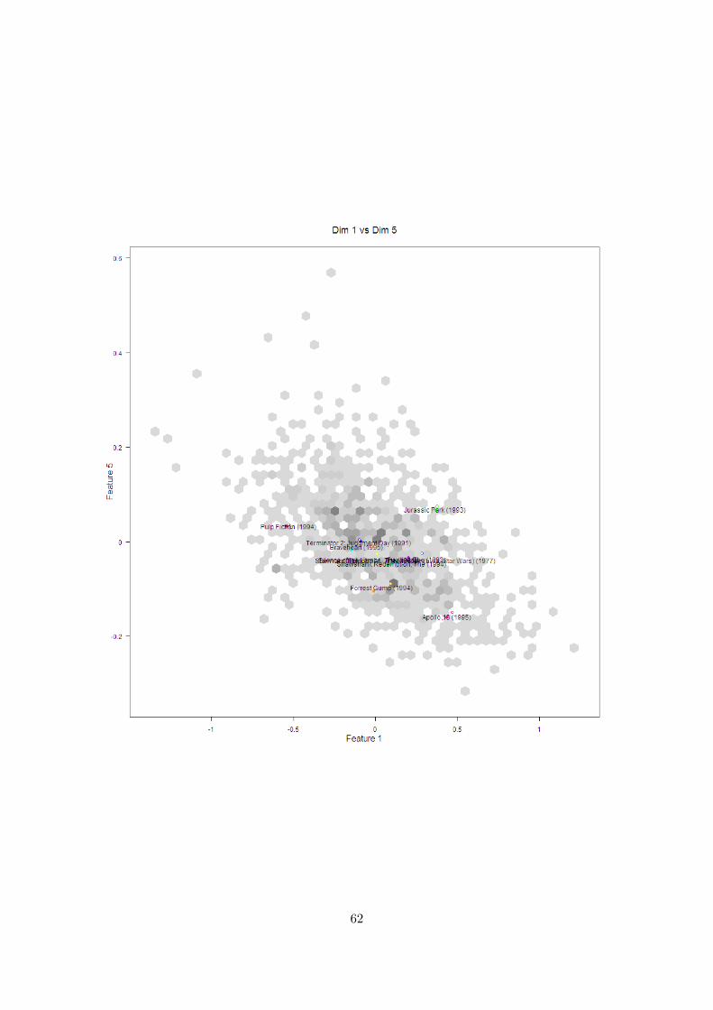
62

Appendix B

Multidimensional Scaling Clusters

63

Tab

leB

.1C

lust

ers

for

Thre

eD

imen

sion

al

Solu

tion

for

Ran

dom

Sta

rtP

erce

ived

Sim

ilari

tyC

on

dit

ion

inC

hapte

r5

Ap

oll

o13

Th

eL

ord

of

Th

eR

ings

IT

he

Lor

dof

Th

eR

ings

IIG

old

enE

yeS

pee

dM

issi

on:

Imp

ossi

-b

leD

ieH

ard

Sta

rW

ars

IVS

targ

ate

Sta

rW

ars

VA

lien

sB

ab

eT

he

Lio

nK

ing

Ala

dd

inB

eau

tyan

dth

eB

east

12

Mon

keys

Batm

anF

orev

erJu

rass

icP

ark

Wate

rwor

ldB

lad

eR

un

ner

Ind

ian

aJon

es:

Raid

ers

ofth

eL

ost

Ark

Ali

enT

he

Mat

rix

X-M

en

Wh

ile

You

Wer

eS

leep

ing

Fou

rW

edd

ings

an

da

Fu

ner

alS

leep

less

inS

eat-

tle

Tit

anic

Sh

akes

pea

rein

Lov

eA

ceV

entu

ra:

Pet

Det

ecti

veT

he

Mas

kH

ome

Alo

ne

E.T

.th

eE

x-

trat

erre

stri

alT

he

Usu

al

Su

s-p

ects

Pu

lpF

icti

on

Th

eF

ugi

tive

Th

eG

od

fath

erR

eser

voir

Dog

sG

ood

fell

asT

he

God

fath

er:

Par

tII

Clu

eles

sD

um

b&

Du

mb

erT

he

Sh

awsh

ank

Red

emp

tion

Sch

ind

ler’

sL

ist

Dan

ces

wit

hW

olve

sB

ein

gJoh

nM

alko

vic

h

64

Tab

leB

.2C

lust

ers

for

Thre

eD

imen

sion

al

Solu

tion

for

Pre

sort

edS

tart

Pre

fere

nce

Sim

ilari

tyC

on

dit

ion

inC

hapte

r5

12

Mon

keys

Wate

rwor

ldE

.T.

the

Extr

a-T

erre

stri

alB

ab

eT

he

Lio

nK

ing

Ala

dd

inB

eau

tyan

dth

eB

east

Batm

anF

orev

erS

targ

ate

Bla

de

Ru

nn

erA

lien

sA

lien

Clu

eles

sT

he

Usu

al

Sus-

pec

tsA

pol

lo13

Pu

lpF

icti

onT

he

Sh

awsh

ank

Red

emp

tion

Th

eF

ugi

tive

Sch

ind

ler’

sL

ist

Du

mb

&D

um

ber

Ace

Ven

tura

:P

etD

etec

tive

Th

eM

ask

Hom

eA

lon

e

Fou

rW

edd

ings

an

da

Fu

ner

alD

ance

sw

ith

Wolv

esS

hak

esp

eare

inL

ove

Th

eG

od

fath

erG

ood

fell

as

Th

eG

od

fath

er:

Part

IIG

old

enE

yeS

pee

dM

issi

on:

Imp

ossi

-b

leD

ieH

ard

Ju

rass

icP

ark

Raid

ers

ofth

eL

ost

Ark

Th

eM

atri

xX

-Men

Lor

dof

the

Rin

gs

IL

ord

ofth

eR

ings

IIS

tar

Wars

IVS

tar

Wars

VW

hil

eY

ouW

ere

Sle

epin

gS

leep

less

inS

eat-

tle

Tit

anic

65

Tab

leB

.3C

lust

ers

for

Thre

eD

imen

sion

al

Solu

tion

for

All

Con

dit

ion

sin

Chapte

r6

12

Mon

keys

Ap

oll

o13

Wat

erw

orld

Rai

der

sof

the

Los

tA

rkT

he

Mat

rix

X-M

en

Bab

eT

he

Lio

nK

ing

Ala

dd

inB

eau

tyan

dth

eB

east

Batm

anF

orev

erJu

rass

icP

ark

Bla

de

Run

ner

Clu

eles

sD

um

b&

Du

mb

erA

ceV

entu

ra:

Pet

Det

ecti

veT

he

Mas

kH

ome

Alo

ne

E.T

.th

eE

xtr

a-T

erre

stri

alG

old

enE

yeS

pee

dM

issi

on:

Imp

ossi

-b

leD

ieH

ard

Lor

dof

the

Rin

gs

IL

ord

ofth

eR

ings

IIT

he

Sh

awsh

an

kR

edem

pti

onD

ance

sw

ith

Wolv

esB

ein

gJoh

nM

alko

vic

hS

tar

Wars

IVS

tar

Wars

VS

targ

ate

Ali

ens

Ali

enU

sual

Su

spec

ts,

Th

eP

ulp

Fic

tion

Th

eF

ugi

tive

Th

eG

od

fath

erR

eser

voir

Dog

sG

ood

fell

asT

he

God

fath

er:

Par

tII

Wh

ile

You

Wer

eS

leep

ing

Fou

rW

edd

ings

an

da

Fu

ner

alS

chin

dle

r’s

Lis

tS

leep

less

inS

eat-

tle

Tit

anic

Sh

akes

pea

rein

Lov

e

66

References

Balabanovic, M., & Shoham, Y. (1997). Fab: content-based, collaborative recommendation.Commun. ACM , 40 (3), 66–72.

Bollen, D., Knijnenburg, B. P., Willemsen, M. C., & Graus, M. (2010). Understanding choiceoverload in recommender systems. In Proceedings of the fourth acm conference on recom-mender systems (pp. 63–70). New York, NY, USA: ACM.

Carroll, J. D., & Chang, J.-J. (1970). Analysis of individual differences in multidimensional scal-ing via an n-way generalization of eckart-young decomposition. Psychometrika, Volume35 , 283–319.

Chandler, D. (n.d.). Introduction to genre theory. Available fromhttp://www.aber.ac.uk/media/Documents/ intgenre/chandler genre theory.pdf

(Web. 26 Nov 2009)Cox, T. F., & Cox, M. A. A. (2000). Multidimensional Scaling, Second Edition. Chapman &

Hall/CRC. Hardcover.Dijksterhuis, A., Bos, M. W., Nordgren, L. F., & Baaren, R. B. van. (2006, February 17).

On Making the Right Choice: The Deliberation-Without-Attention Effect. Science,311 (5763), 1005–1007.

Drolet, A., & Luce, M. F. (2004). The rationalizing effects of cognitive load on emotion-basedtrade-off avoidance. Journal of Consumer Research, 31 , 63-77.

Fasolo, B., Hertwig, R., Huber, M., & Ludwig, L. (2009). Size, entropy, and density: What isthe difference that makes the difference between small and large real-world assortments?Psychology and Marketing , 26 (3), 254-279.

Hennig, C. (2008). Dissolution point and isolation robustness: Robustness criteria for generalcluster analysis methods. J. Multivar. Anal., 99 (6), 1154–1176.

Herlocker, J. L., Konstan, J. A., Terveen, L. G., & Riedl, J. T. (2004). Evaluating collaborativefiltering recommender systems. ACM Transactions on Information Systems, 22 (1), 5–53.

Hollins, M., Faldowski, R., Rao, S., & Young, F. (1993). Perceptual dimensions of tactile surfacetexture: A multidimensional scaling analysis. Attention, Perception, & Psychophysics, 54 ,697-705. (10.3758/BF03211795)

Jin, R., Si, L., Zhai, C., & Callan, J. (2003). Collaborative filtering with decoupled models forpreferences and ratings. In CIKM ’03: Proceedings of the twelfth international conferenceon information and knowledge management (pp. 309–316). New York, NY, USA: ACM.

Knijnenburg, B., Meesters, L., Marrow, P., & Bouwhuis, D. (2010). User-centric evaluationframework for multimedia recommender systems. In O. Akan et al. (Eds.), User centricmedia (Vol. 40, p. 366-369). Springer Berlin Heidelberg.

Koren, Y., Bell, R., & Volinsky, C. (2009, August 07). Matrix factorization techniques forrecommender systems. Computer , 42 (8), 30–37.

Kruskal, J. B., & Wish, M. (1978). Multidimensional scaling. SAGE Publications, Inc.Langford, B. (2005). Film genre: Hollywood and beyond. 22 George Square, Edinburgh:

Edinburgh University Press.

67

Lawless, H. T., Sheng, N., & Knoops, S. S. C. P. (1995). Multidimensional scaling of sortingdata applied to cheese perception. Food Quality and Preference, 6 (2), 91 - 98.

McNee, S. M., Riedl, J., & Konstan, J. A. (2006a). Being accurate is not enough: how accuracymetrics have hurt recommender systems. In G. M. Olson & R. Jeffries (Eds.), CHI extendedabstracts (p. 1097-1101). ACM.

McNee, S. M., Riedl, J., & Konstan, J. A. (2006b). Making recommendations better: ananalytic model for human-recommender interaction. In G. M. Olson & R. Jeffries (Eds.),CHI extended abstracts (p. 1103-1108). ACM.

Melville, P., Mooney, R. J., & Nagarajan, R. (2002). Content-boosted collaborative filtering forimproved recommendations. In Eighteenth national conference on artificial intelligence(pp. 187–192). Menlo Park, CA, USA: American Association for Artificial Intelligence.

Murtagh, F. (1983, November 1). A Survey of Recent Advances in HierarchicalClustering Algorithms. The Computer Journal , 26 (4), 354–359. Available fromhttp://dx.doi.org/10.1093/comjnl/26.4.354

Novello, A. (2009). Perceptual and algorithmic evaluation of inter-song similarity in westernpopular music. Unpublished doctoral dissertation, Eindhoven University of Technology,Eindhoven.

Payne, J. W., Bettman, J. R., & Johnson, E. J. (1993). The Adaptive Decision Maker. Cam-bridge University Press. Paperback.

Pazzani, M. J., & Billsus, D. (2007). The adaptive web. In P. Brusilovsky, A. Kobsa, &W. Nejdl (Eds.), (pp. 325–341). Berlin, Heidelberg: Springer-Verlag. Available fromhttp://portal.acm.org/citation.cfm?id=1768197.1768209

Pham, M. T. (1998). Representativeness, relevance, and the use of feelings in decision making.Journal of Consumer Research, 25 , 144-159.

Rendle, S., Tso-Sutter, K., Huijsen, W., Freudenthaler, C., Gantner, Z., Wartena, C., et al.(2009). MyMedia Deliverable 4.1.2 State-Of-The-Art recommender algorithms. Availablefrom http://www.mymediaproject.org/Publications/

WP4/D4.1.2-stateoftheart.pdf

Shepard, R. N. (1963). Analysis of proximities as a technique for the study of informationprocessing in man. Human Factors, 5 (33), 33-48.

Shepard, R. N. (1980, October 24). Multidimensional scaling, tree-fitting, and clustering.Science, 210 (4468), 390–398.

Tsogo, L., Masson, M. H., & Bardot, A. (2000). Multidimensional Scaling Methods for Many-Object Sets: A Review. Multivariate Behavioral Research, 35 (3), 307–319. Available fromhttp://dx.doi.org/10.1207/S15327906MBR3503 02

Ziegler, C.-N., McNee, S. M., Konstan, J. A., & Lausen, G. (2005). Improving recommendationlists through topic diversification. In WWW ’05: Proceedings of the 14th internationalconference on world wide web (pp. 22–32). New York, NY, USA.

68