eindhoven university of technology master preliminary … · user- and programmers manual structure...
TRANSCRIPT

Eindhoven University of Technology
MASTER
Preliminary user- and programmers manual structure identification program IPMSID
Tchang, C.C.
Award date:1986
DisclaimerThis document contains a student thesis (bachelor's or master's), as authored by a student at Eindhoven University of Technology. Studenttheses are made available in the TU/e repository upon obtaining the required degree. The grade received is not published on the documentas presented in the repository. The required complexity or quality of research of student theses may vary by program, and the requiredminimum study period may vary in duration.
General rightsCopyright and moral rights for the publications made accessible in the public portal are retained by the authors and/or other copyright ownersand it is a condition of accessing publications that users recognise and abide by the legal requirements associated with these rights.
• Users may download and print one copy of any publication from the public portal for the purpose of private study or research. • You may not further distribute the material or use it for any profit-making activity or commercial gain
Take down policyIf you believe that this document breaches copyright please contact us providing details, and we will remove access to the work immediatelyand investigate your claim.
Download date: 27. Jun. 2018

EINDHOVEN UNIVERSITY OF TECHNOLOGY
Faculty of Electrical Engineering (EE)
Group Measurement and Control ( ER)
PRELIMINARY
USER- AND PROGRAMMERS MANUAL
STRUCTURE IDENTIFICATION PROGRAM
I P M SID
by C.C. Tchang
This report is submitted in partial fulfillment of therequirements for the degree of electrical engineer (M.Sc.) atthe Eindhoven University of Technology.The work was carried out from October 1985 until October 1986in charge of Prof.Or.Ir. P. Eykhoff and under supervision ofIr. P.H.M. Janssen and Dr.Ir. A.J.W. va~ den 800m.
The Faculty of Electrical Engineering of the Eindhoven Universityof Technology does not accept any responsibility regarding thecontents of students practical work- and graduation reports.
De faculteit der Elektrotechniek van de Technische UniversiteitEindhoven aanvaardt geen verantwoordelijkheid voor de inhoudvan stage- en afstudeerverslagen.

1 .0
LIST OF CONTENTS=======::=-===-=====
Introduction .
Page
3
PART I : USE R MAN U A L
1.01.11.2
II. 0II.1
II. 2II.2.1
II. 3II. 4II. 5
==============================
General program structure .List of questions .Making plots with plotprogram GRA .
PART II : PRO G RAM MER SMA N U A L============================================
Survey of available software .Organisation of the main software .
Efficient use of memory .The bookkeeping algorithm .
Recursive calculation of SPossible future extensionsHow to compile the pro2ram
2
56
1 1
1314
1616
181920

1.0 INTRODUCTION
The program IPMSID performs the structural identification oflinear multivariable systems in canonical observability formusing the (instrumental) product moment (IPM) method.IPMSID supports the Tollowine choices aT instrumental variables:
1) Output samples2) Delayed input samples3) Filtered input samples
( PM)( IPM)( IPM)
The method used for structural identification uses the GUIDORZIform. The HERMITE- and DIAGONAL form are not supported yet.
Two singularity tests have been implemented:
1) Determinant ratio2) Least singular values
The program and routines have been developed on the VAX 11/750and MICROVAX computers and are written in FORTRAN 77.No adaptations have been made for the STANDARD FORTRAN 77 compiler,so only the OLDFOR-option can be used to compile the program.
The two partsdescription of'routines:
ofthe
this preliminary manualstructure identification
give aprogram
thoroughand its
PART I (USER MANUAL) gives the information required to run theprogram on a VAX-computer. It gives explanations on questionsposed in the program. Also information is given about how to makeplots with GRA.
PART II (PROGRAMMERS MANUAL) gives information aboutsoftware. Not only we shall give additional informationsome implemented algorithms but also how to compile theand possible future extensions.
For more information about the IPM-method is referred to:
theabout
program
- Tchang C.C. (1986)Structural identification of multivariable systemsin canonical form using the instrumental product momentCIPM)-matrix method.M.Sc. Thesis, EUT October 1986.
- 8 e k k e r s C. F . P . M. (1 985)Structure and parameter identification of multivariablesystems represented by matrix fraction descriptions.M.Sc. Thesis, EUT August 1985.
3

The program is based on the program STRUCID written by F.Bekkers.The basic program has been revised and extended with some newroutines.The most important extensions are:
1) Choice of delayed and filtered inputs as IV2) Optimalisation in speed and memory usage3) New options in filling the matrices Z and OMEGA
Different versions of IPMSID are available at this moment:
Version 1.0 (VAXRC2: :USER1:[ELERCHEN.IPMSTRUCID]IPM10.EXE;1) isthe first version, which actually builds up Z and OMEGA fromSYSIO and stores them in two big arrays (Array SYSIO contains themeasured data on p inputs and q outputs). Each (instrumental)product moment matrix S is calculated by multiplyingZ(transposed) with OMEGA. Because of the number of samples andthe storage of the arrays the calculation is a time- andmemoryconsuming process. The storage of an array with 3000samples * 60 columns requires e.g. 1.44Mbyte.
In version 2.0. (THEEL1: :DISK2:[ERMIMCHEN.IPMOLD]IPM20.EXEj1)the singularity tests have been optimized in speed and memory usage.This has been achieved by:
1) Direct calculation of the elements of S out of SYSIO.This requires an intelligent bookkeeping system,whichtracks the begin- and endtime indices.
2) Using a dimensionally recursive algorithm in the case ofdeterminant ratio to yield the det.ratio.This makes an explicit calculation of determinantsredundant.This algorithm also delivers a begin estimationof the parametervector.
In version 2.1. (THEEL1: :DISK2:[ERMIMCHEN.IPMSTRUCIDJIPMSID.EXEj1)an own debug-mode has been implemented in order to give a quickview of important bookkeeping vectors and IPM-matrix S during thesingularity test.
Note that when the det.ratio test is used not Sbut its inverse will be displayed !! I !
***
Because of possible bugs in the old software, *as this has not been updated, it is recommended *to use the latest version of the program. *
4

I PART I : USE R MAN U A L
This manual gives the user the necessary inTormation to RUN thestructure identification program IPMSID. When only Tew inputvalues are changed in successive runs, it is recommended to useBATCH-files (.COM). Since the program can be divided in someseparate blocks we will give explanations on non-trivialquestions, which may be posed. ATter this some inTormation willbe given about the use of plotprogram GRA.
1.0 General program structure
The program has been divided into several blocks which are givenin the next flowdiagram:
~(ENTER VALUESA~ FOR THE ESTIMATION]
l--> {Group 1: Inputs,outputs,samples}~> {Group 2: Filenames}I
[PREPROCESSING OF THE SIGNALS) {Group 3}
[ENTER INFOR~ATION DEPENDENT ONCHOICE OF INSTRUMENTAL VARIABLES]
~ {Group 4: IV-inTormation}~ {Group 5: Singularity test inTo}
(MENU TO DISPLAY ENTERED GROUPSOF VARIABLES OR START/EXIT PROGRAM]
I
IPM STRUCTURAL IDENTIFICATION
DISPLAY NAMES OF JILES WITH RESULTSAND ASK FOR ANOTHER RUN
EJ_------------51
-----------------"

INPUT FILE(S)
OUTPUT FILE(S)
DATA FILE WITH INPUT/OUTPUT SAMPLES(CREATED BY E.G. SIMUL) IN MATLABOR THE-STRUCTURED FORMAT.
PRINTFILE WITH RESULTS OF ESTIMATIONPLOTFILE WITH RESULTS IN GRA-FORMAT
I. 1. List oT questions
In this paragraph we will give a list oT all the questions whichmay appear in the program. A short explanation will be givenat some non-evident options.
\ beTore a question denotes that this questions occursdependent on a choosen option.
The variable between parenthesis at the end oT each linecorresponds with the name oT the variable associated withthe question in the program.)
BLOCK 1 : ENTER VALUES AND NAMES FOR THE ESTIMATION*****************************************************************
Do you want to use the IPMSID DEBUG-mode ? ( DBMODE)
IPMSID contains its own DEBUG-mode. In this mode one can displayall important BOOKKEEPING-vectors and the IPM-matrix S during thesingularity test.In this way one can view the changes and veriTythe perTormance oT the bookkeepingalgorithm.This handy toolreplaces the VAX-DEBUGGER and is less time-consuming.
Do you want system names Tor all the diTTerent Tiles made in theprogram or do you want to enter the names yourselT ? (INAME)
It is possible to let the program assemble Tile-names Trom thename oT the INPUT-OUTPUT data Tile, created by the simulationproEram SIMUL. In this case the SIMUL-Tile should be coded asTollows:
1234567XXYYYZZ.DAT
XXYYY
ZZ
= process code e.g. F3= 3 character code Tor
in the data TileSignal Noise ratio in
6
= Tirst order system 3the number OT samples
dB

The names of the resulting files are created as follows:
Files with estimation results:
File with plot results in GAA-Tormat:
123456?S90AS_XXZZWWW. OAT
123456?S90PL_XXZZWWW.OAT
The character put onchoosen singularity test
position 3 is determinedo = determinant ratioS = singular values
by the
The 3 character code WWW corresponds with the number ofsamples used for the estimation and must be entered atthe question:
\Enter a 3-character code for the number of samples (CODE)---------------------------------------------------------e.g. 1T? = 1?OD samples, 5H2 = 520 samples
Enter the number aT inputs?
Enter the number aT outputs ?
( IP)
( IQ)
Enter the number of samples used for the estimation? (NSAMP)
Enter the index of the start sample ( NAECBG)
The start sample is the number of the first sample in the IO-datafile which is to be used for the estimation. This choice offersthe possibility to select a desired interval out of a set ofavailable data.
Enter the name of the file which containssamples:
This file is created by e.g. SIMUL.
the INPUT/OUTPUT(FILNM1)
Enter the structure of the file with the lO-samples:
[0] THE-structure[1] : MATLAB-structure
?
( FILSTAUC)

jEnter the name of the file for the storage of the FINAL RESULTS:( FILNM2)
(Overview of the entered system parameters and the results of thestructure identification).
jEnter theRESULTS:
name of the file for the stora2e of the PLOTABLE( F ILNM3)
(F( S) as a function of the structure parameters).
BLOCK 2 : PREPROCESSING**************************~~**************************************
00 you want to correct the results with their mean value ?(ICORR)
If this option is choosen, the mean valueinterval (NRECBG,NRECBG+NSAMP-1) willcorrection will be performed on all the( 1 , NRECBG+NSAMP-1 )
of the samples in thebe calculated. The
samples in interval
Enter the number of the multiplication factor that you want tochange: Enter [0] if they are correct. (MULTO(I)
It is possible to multiply each output by a desired factor.
Do you want to estimate the D-matrix ? ( IESTD)
This is the D-matrix in a state-space model of the process.
A coarse estimation is given by (Carriere 1984):
crosscorr( u,j, Y:J. , tau=O )D(i,j) =
autocorr( U,j , tau=O)
with u,j = 'preprocessed' input j
Y:J. = 'preprocessed' output i
Do you want to perform the D*U correction on the outputs? ( ID)-----------------------------------------------------------------So
8

OF3 ENTER INFORMATION DEPENDENT ON THE CHOICEINSTRUMENTAL VARIA8LES.
*****************************************************************
BLOCK
How do you want to choose the instrumental variables? (IVCH)-----------------------------------------------------------------[ 1] Output samples[2] Delayed input samples[3] Filtered input samples
* DELAYED INPUT SAMPLES *
/Which delayed inputs do you want to use as IV ? ( ICH)-----------------------------------------------------------------[0] Output i = Delayed input i[1] : Own choice ( Output i = Delayed input j with i#j)
[0] Output 1 = Delayed input 1, Output 2 = Delayed input 2, etc.If IQ>IP then Output IP+1 = IP, Output IP+2 = IP+1, etc.
//Enter the number of the delayed input for output i: ( IPLA( i) )-----------------------------------------------------------------It is possible to select all inputs once or more to use asdelayed input.
/Enter delay in sample times: ( TAU)
It is possible to choose a delay between in interval [0,9].Normally a delay equal to 1 is choosen.
/00 you want to use information from the past in the IV's? (HIS)
In case of delayed inputs samples like U(NREC8G-1) ,U(NREC8G2) ,U(NREC8G-3) etc. may be shifted into matrix Z. These samplesare in fact 'not measured' but available when the start sample ischoosen > 1. When no information from the past is required thenU(NREC8G-1), U(NRECBG-2), U(NREC8G-3) etc. will be made zero.
FILTERED INPUTS
/Enter the number of the start sample forsamples
the filtered input( IVBEG)
This start sample must be choosen between 1 and NRECBG.The structural estimation starts at sample NREC8G. The IVfiltering of inputs at IVBEG. So NREC8G-IV8EG samples are alsobeing filtered but not used for the estimation. These samplesare used to set the initial conditions of the filter which isgiven in state-space form.
9

/Enter the name of the file, which contains the filter matrices:( FFILNM)
The filtermatrices should be available in state-space format.
/Enter the structure of the matrix-file: ( FILSTRUC)-----------------------------------------------------------------[0] THE-structure[1] : MATLAB-structure
SINGULARITY TEST INFORMATION
Enter the number of the method you intendsingularity test of S:
[ 1] Determinant ratio method[2] : Least singular value method
Enter the maximum of row degrees to be tested
to use for the( CAL VAL)
( MTSTNU)
Initially it is recommended to choose MTSTNU as high as possible(9) to get a view of the system order.
Enter way to fill OMEGA and Z (number of rows) ( OPTION)
The number of rows in these matrices can be choosen fixed orvariable. Consider the following structure with k=NRECBG:
u(k) u(k+1)u( k+1)
u( k+OEL TA( i)-1)
2->
1-> u( k+N-1)r. u( k+N)
u(k+N+OELTA(i)-2)
Not ice that samp Ie s u( k+N+ 1) ,u( k+N+2) , .. ,u( k+N+OEL TA( i) -1 arefuture samples and therefore not available (not measured).
When the 'fixed' option is choosen the program will calculatethe matrices to position 2, which row contains the last measuredsample U( k+N-2) .The final number of rows will be:
MIN{ N-OELTA(i)+iJ ).1~i~IP+IQ
10

When the 'variable option' is choosen the matrices will be filledto position 1. All not available samplesU(k+N+1) .... U(k+N+DELTA(i)-2 will be made 0 (Number of rows willbe N)
NOTE that choosing a variable number of rows will affectnumber of multiplications and therefore the calculation o~
covariance (calculation of an element of S). This mayerrors during recursive calculation of S.
thethe
cause
Enter theidentification:
threshold value for the structural( VALeRI)
00 you want a fixed or variable threshold ? ( IVAFIX)
Fixed: The threshold value willsingularity tests.Variable: Before each singularity testbe entered.
DISPLAY OF ENTERED PARAMETERS
be constant during all
a new threshold value must
Enter the number of the group if you want to to display or tochange something in that group: (IGROUP)
[1] Inputs, outputs, samples[2] File names[3] Preprocessing[4] IV-information[S] Singularity test information[6] Display all groups[?] No changes, start identification[8] Exit from IPM- structure identification program
1. 2. MAKING PLOTS WITH PLOT PROGRAM GRA
In this paragraph we will make an AS-plot of a plotfile createdby IPMSID using GRA. It is off course possible the choose otheroptions (A4 format etc.), but the choosen options are adequateand convenient for a good representation of the results.The plots have been made on a ?221S-HP plotter.When VT 220 or VT 240 terminals (or emulations of these)terminalsare used the call of GRA should be proceeded with:
>SET TERMINAL VT/S2 to put these terminals in graphic-mode.
Gra can be called by entering:
>GRA
1 1

We shall now give a list of answers on questions posed for makinga AS-plot of our plotfile.
**********************************************************
Name of the file to be read PL_XXZZWWW.DATor own name
Do you want to read a measurepoint file?: N
Structure of the DATA-file GRA-structureThe file does have the predefined structure.
Variables which have to be plottedVariable 1 =Variable 2 =
Text of variable 2or
X-variable2 <RETURN>
10LOG(DET.RATIO)10LOG(L.S.V.)
number of samplessignal/noise ratioprocess codestruct.identification
Text headinge.g.
Text X-axisIdentification
IPM -----------------------IPM delayed inp. est.int.500-1500STRUCTURESIF3601T
I~System of axisGrid lines verticalLimitations X-min
X-maxwith
( e. g
X linearlY linearYshould be 0should be {MTSTNU*(IP+IQ)}-1IP number of inputsIQ = number of outputs
MTSTNU = maximum order to be testedV-min depends on plot
if you want to plot more plots in one figure)V-max 0
Plot sizeTop/Bottom A4
ASdependent on e.g sing. test
Angle scale value to the axis : X-axisY-axis
o degreeso degrees
Discrimination method in case of more variablesown choice
12

I PART II PRO G RAM MER S MAN U A L I11.0 Survey oT available sOTtware
----------------------------Main program
Name :Directory
Routines
1PMS1D.EXE;1THEEL1: :DISK2:[ERMIMCHEN.1PMSTRUC1D]
All FORTRAN-version of the routines are available inTHEEL1: :D1SK2:[ERM1MCHEN.1PMSTRUC1D.FORF1LES]
All OBJECT-files have been stored in library :THEEL1: :D1SK2:[ERM1MCHEN.IPMSTRUCID]IPMBIB.OL8;1
*************************************************************** All routines between f ... f are only used in older versions ***************************************************************
CALCMfCALDETf
CALRMTDUCORREST1MDfF1LLOMf
fFILLZ/
MEANSD
RDlOMLSVDECTSTSlN
calculates a new column to add to Scalculates the absolute value of thedeterminant of square matrix S.calculates a new row to add to Sperforms the D*U correction on the outputs.estimates the D-matrixTills the matrix OMEGA with in- andoutput data from SYS10.Tills the matrix Z with process inputsamples from SYSIO and instrumentalvariables.calculates mean over NSAMP samples andcorrects if wanted with this value.Calculates standard deviation simultaneously.reads an 10 file in MATLAB-format in SYSIOdecomposition in singular valuestest singularity of matrix S iT det.ratio orleast singular value less than threshold thenthe matrix is 'singular'
THE-structure routines
RDHETHEF02RDIOTHEF01RDSSTHEF01
reads heading ofreads lO-samplesreads a statestructured file.
13
a THE-structured filefrom a THE-structured filespace model from a THE-

SIMUL-routines
(These routines are used for the filtering of inputand have been copied from SIMUL)
signals
RDSYSRDDATAERRORRDWRMASCHRMASIMDUT
reads a system into an arrayreads data into the programwrites error messages to the screenreads and writes a matrixwrites a matrix to the screensimulates a system in state-space format
Overlay structures
All routines which use one or more other routines are given inthe diagram below :
NAG FD3AAF NAG F02WDF
II.1 Organisation of the main software
The general structure of the program has been given inI.O.. We shall give another structure based(version 2.1) and a flow diagram of the IPMidentification process.
USERMANUALon labelsstructure
LABEL
1000-18002000-25003000-3?003800-40004000-43004500-49005000-5100
6000-6900?000-?9008000-88009000-9950
BLOCK
Enter system parametersPreprocessingIV-informationFiltering of inputsInformation for the singularity testWrite entered values to screenWrite entered values to file andinitialise vectors and arraysDeterminant ratio methodSingular value methodReserved for new singularity testList of formats
14

FLOWDIAGRAM IPM STRUCTURE IDENTIFICATION----------------------------------------
\\ Initialise vectors and S \
I\ Calculate se 1,0, .. ,0)\
II Max order tested?
Iy------~
Calculate columns of OMEGA and Zand S=Zetransposed)*OMEGA
\I Calculate det{S} or LSV{S} II
I detratio {S} or LSV {S} < Threshold ?I
N Iy
I Fix invariant I.... < II NEXT ORDER
For detailed information we refer to the comments in thelisting of the program.
15

11.2. Efficient use of memory
The structural identification process consists of thedetermination of the 'near' singularity of the 1PM-matrix S (orits inverse Q) which is build up from Z and OMEGA. Eachincrement of a DELTA corresponds with an increment of 5 withone row and one column. 50 the new S is the previous 5 with onerow and one column added to its ends.When 'singularity' has beendetected the last incremented DELTA will be decremented and keptconstant during the continuation of the estimation.Also the lastjoined row and column in S will be overwritten (discarded).
11.2.1 The bookkeeping algorithm
Before we will discuss the algorithm of the bookkeeping system weshould have a look at the structure of the matrices Z and OMEGA.
Consider for simplicity a S1SO-observation-matrix OMEGA:
u( 1)u( 2)u( 3)
I u( N)l-
u( 2)u( 3)u( 4)
u( N+ 1)
u(O(1)) I y( 1) y( 2) y( eS( IP+IQ) )u( eS( 1) +1) I y( 2) y( 3) y( eS( IP+IQ) + 1)u( o( 1) +2) I y( 3) y( 4) y( eS( IP+IQ) +2)
II
u( eS( 1) +N-1) I y( N) y( N+ 1) y( eS( IP+IQ) +N-1)
When we have a closer look we observe that the second columnconsists of the elements of the first column shifted one positionin time. In both directions from the upper left position to theright or downwards the time index is incremented. This leads tomultiple storage of identical samples. The same applies to matrixZ .
For efficient storage we actually need to store the followinginformation (Consider matrix OMEGA)
1) Vector with columnreferences in SYSIO:
CREFO = •• lil •••• 1 p+1 1 •••.••• 1 p+l ]
j-th column in OMEGA
50 the j-th column in OMEGA consists of elements of column i in5Y5IO
16

2) Vector with timeindices of first row in OMEGA: (OIN8EG)----------------------------------------------
First row --> u( 1) u( 2)
OMEGA =
u( OROWS( 1) )
. u( DEL TA) y( 1) y( DEL TA)
3) Vector with number of rows for each column in OMEGA (OROWS)
NOTE that the number of ROWS is not one number !Because zero's can be introduced in a column amultiplications can be left out. This number isfrom ROWS and saved in OROWS.
number ofsubstracted
Defining the same vectors (CREFZ,ZINBEG,ZROWS) for Z, we may thenuse the following algorithm:
1) Determine reference column in SYSIO by using the value ofINU, which denotes the concerning in- or output.Filtered inputs are stored in the columns IP+IQ+1 upto andwith IP+IQ+IQ of SYSIO.Store columnreference of Z in CREFZ(ISIS) and OMEGA inCREFO( ISIS)
STRUCTURE OF SYSIO:
<----------------------IP+IQ+IQ columns------------------->
E.IP inputs .. >\ < .. IQ outputs .. >1 < .. IQ filtered input~
An advantage of this structure is that filtered inputs canbe obtained by simply adding an offset to the concerningpointer( s) .
2) Determine start index of last added column in Z and OMEGA.The value of DELTA(INU) gives the number of shifts fromfirst sample SYSIO(NSTART,INU).
The start index of the last added column in Z and OMEGA is:Output samples and filtered inputs --> DELTA(INU)-1Delayed input samples --> 1-DELTA(INU)For each increment of INU these values are storedin the arrays OIN8EG(ISIS) and ZINBEG(ISIS).
17

When using delayed inputs it is possible (option HIS(tory)) touse information of 'past' samples for the estimation. Thesesamples are available when one starts at NRECBG>1. When no use ismade of past samples these position will be filled with zero's.The implementation of this option is done by adjusting a vectorZINCOR. The elements give the number of positions which should bediscounted from calculation.
3) Determine the number of rows in each column of theand OMEGA. This is determined by the option ofvariable number of rows: The number of rows isvariable ROWS. From each new added column theavailable samples in SYSIO is compared with ROWS.of these is stored in ZROWS(ISIS) or OROWS(ISIS).(ISIS = dimension of S)
matrices Zfixed orgiven by
number ofThe minimum
We can now calculate S=Z(transposed * OMEGA).shall do this recursively.
To gain time we
11.3 Recursive calculation of S
Matrix S = ZT.OMEGA is now to be extended by one row andone column
S = :] * r U(k l ]N U(k)T L
[ c ]cc
N r r r d
c consists of (all rows of ZT correlated with thelast added column in OMEGA (Routine CALCM)
r consists of the last added row in ZT correlated with(all columns of OMEGA)-1 (Routine CALRMT)
d consists the 'covariance' of the last addedvector.
18

Because of offset-correction the first row of ZT and first columnof OMEGA are filled with a vector 1.
NOTEwherebein2to n,
that the number of matrixelements to be calculated is 2n+1n is the dimension of matrix S. When output samples ar~
used as IV, the number of elements to be calculated reducesbecause of symmetry (c=r) .
So the
11.4.
extension of matrix S can be described by:1) Increment DEL TA( i)2) Calculate start- and endtime indices of
last added column(s) in nand Z3) Calculate 'covariance'4) Correlate (all rows of ZT)-1 with last
added vector in OMEGA5) Correlate (all columns of OMEGA)-1 with
last added row in ZT6) Adjust bookkeeping vectors.
Possible future extensions
We will give a list of possible future extensions:
1) Other parametrizations, like HERMITE- and DIAGONAL form.2 ) New sin 2 u 1 a r it y te s t s3) New preprocess operations4) Processing of the parameter vector obtained in det.ratio
The label structure given on page 14 offers a flexible insertionof new routines and pr02ram lines. Whereever possible incrementsof 10 have been used in labelnumbers. Each block is preceededwith some comment and difficult passages are also commented.The programming is done according to 'standard' ER pr02rammingrules, which are given in (in Dutch)
Beckers W."Afspraken en richtlijnen voor het programmerenin FORTRAN ?? op een VAX computer"EUT, Group ER, Dec. 16, 1985
19

11.5. How to compile the program
Two COMMAND-files are available to compile the program in BATCH
1) FOR.COM2) FOROB.COM
FOR. COM
create an executable filecreate an DEBUG executable file
$ SET OEF [ERMIMCHEN.IPMSTRUCIO]$ OLOFOR/LIS/F?? IPMSIO.FOR;1$ LINK IPMSIO,IPMBIB/LIBRARY$ DELE IPMSID.OBJ;1$ DELE IPMSID.MAP;1$ LO
FORDB.COM
$ SET DEF [ERMIMCHEN.IPMSTRUCID]$ OLDFOR/DEBUG/NOOPTIMIZE/LIS/F?? IPMSID.FOR; 1$ LINK/DEBUG IPMSIO,IPMBIB/LIBRARY$ DELE IPMSID.OBJ;1$ DELE IPMSID.MAP; 1$ LO
These program can be started with:
>@GO
>@GODB
GO.COM
or with
$ SUBMIT/KEEP/NOPRINTER/CPUTIME=00:05:00.00 FOR.COM
GODB.COM
$ SUBMIT/KEEP/NOPRINTER/CPUTIME=00:05:00.00 FORDB.COM
*******************************************************************
NOTE that the .COM-files explicitly need versionIPMSIO.FOR;1. This means that each edited IPMSIO
should be renamed to IPMSID.FOR;1 !
***
************************************************i~****************
20

EINDHOVEN UNIVERSITY OF TECHNOLOGY
Faculty of Electrical Engineering (EE)
Group Measurement and Control ( ER)
Structural identification ofmultivariable systems incanonical form using theinstrumental product moment
(IPM)-matrix method.
by C.C. Tchang
This report is submitted in partial fulfillment of therequirements for the degree of electrical engineer (M.Sc.) atthe Eindhoven University of Technology.The work was carried out from October 1985 until October 1986 incharge of Prof.Dr.Ir. P. EykhoTT under supervision OTIr.P.H.M. Janssen and Dr.Ir. A.J.W. van den 800m.
The Faculty oT Electrical Engineering oT the EindhovenUniversity of Technology does not accept any responsibility forthe contents of student practical work- and graduation reports.
De faculteit der Elektrotechniek van de Technische UniversiteitEindhoven aanvaardt geen verantwoordelijkheid voor de inhoud vanstage- en afstudeerverslagen.

SUMMARY
We have studied a heuristic systematical procedure for thestructural identification of stable, linear, time-discrete,time-invariant multivariable systems, represented incanonical form, in an environment with high external noiseof unknown statistics.The procedure is based upon the determination of thestructural indices, which specify the complexity of thesubsystems. These indices will be obtained by checking thenear-singularity of a sequence of instrumental productmoment (IPM) -matrices, using the determinant ratio methodand the least singular value method.
The method has been implemented on the MICROVAX II computerfor the Guidorzi-MFD (Matrix Fraction Description) form. Thesoftware has been written in FORTRAN ?? (without VAXextensions) .
In order to get an idea of the performance of thismethod under different conditions, we have performed anumber of simulations on simple test systems, in order tojudge whether this method is sufficiently reliable foruse in practical situations.We have considered i.a. different choices of IV's (delayedand filtered inputs) ,dependencies on the number of samples,different signal to noise ratios, influences of choice ofestimation interval.
Using delayed inputs as instrumental variables, the resultsindicated that a proper detection of the structural indicesis difficult, in case that the noise level is high, becausethe test statistics are fluctuating for structural indiceslarger than the true ones. Using filtered inputs as IV, thechoice of a filter will substantially affect the selectionprocedure.
2

Samenvatting
Het onderwerp van studie is een heuristische procedure voorde structurele identificatie van stabiele, lineaire, tijddiscrete, tijd-invariante multivariabele systemen,gerepresenteerd in kanonieke vorm, in een omgeving met hogeruis met onbekende eigenschappen.
De procedure is gebaseerd op de bepaling van de structureleinvarianten, die de complexiteit van de subsystemenspecificeren. Deze indices worden verkregen door onderzoekvan de 'bijna singulariteit'van een reeks van instrumenteleprodukt moment (IPM)-matrices door middel van eendeterminant ratio test of een kleinste singuliere waardetest.
De methode is geimplementeerd op de MICRDVAX II computervoor de Guidorzi-MFO (Matrix Fractie Oescriptie) vorm. Deprogrammatuur is geschreven in FORTRAN ?? (zonder VAXextensies) .
Om een indruk te krijgen van de prestaties van de methodeonder verschillende omstandigheden, zijn een aantalcomputer simulaties uitgevoerd. Het uiteindelijke doel was:het bekijken of de methode voldoende betrouwbaar is voortoepassing op data uit de praktijk.
Onder andere zijn bekeken verschillende keuzes van IV's,(specifiek: vertraagde en gefilterde ingangen), invloed vanhet aantal gekozen samples, verschillende signaal/ruisverhoudingen, invloed van keuze van het schattingsinterval.
De resultaten, verkregen met vertraagde ingangen alsinstrumentele variabelen, tonen aan dat een degelijkedetektie van de structuur indi~es, in geval van hogeruisniveaus, moeilijk is, omdat de test criteria eenfluctuerend gedrag vertonen voor structuren groter dan deechte structuur. Met gefilterde ingangen als IV wordt deselektie procedure in hoge mate beinvloed door de selektievan het filter.
3

LIST OF CONTENTS
1 . Introduction 6
2.
2. 1 .• 1
.2
2.2.. 1
.2
.3
3.
Model representation and the use of canonicalobservability forms 10
Important model types 10The state-space description 11The matrix-fraction description 11
Canonical forms 12Derivation of the Guidorzi-form forstate-space models 13Transformation to the GuidorziMFO-canon ica 1 form....... . . . . . 16Other MFO-canonical forms............ 21
Structural identification 24
3. 1 .
3.2.. 1.2.3
3.3.
3.4.
4.
4.1 .
Developments
SISO (I)PM-order estimation .Problem definition .The product-moment (PM) matrix .The instrumental product-moment (IPM) matrix
MIMO IPM-structural identification
Choice of instrumental variables
Singularity tests
The determinant method
24
25252628
29
32
34
34
4.2.. 1.2
The determinant ratio method 36Recursive calculation of the determinant ratio. 3?An interpretation of the determinant ratio .... 38
4.3. The least singular value method 41
5.
5. 1 .5.2.5.3.
Data preprocessing 45
Necessity of preproce9sing 45Coarse estimation of O-matrix 46Influence and elimination of off-sets 46
4

6.
6. 1 .6.2.
6.3.6.4.
7.
Computer program development SO
General structure of the program SOOptions 52
Optimization of speed and memory use 53Interpretation of results 53
Performance study by means of simulations 55
7.1.1. 2
7.2.
. 1
. 2
.3
7.3 .
Choice of test systems .Choice of instrumental variables .
SISO-simulations with output samples as IV
Influence of the number of samples .Dependencies on the signal to noise ratio .Influence of choice of estimation interval
SISO-simulations with delayed inputs as IV
S6S7
58
5859S9
59
. 1 Influence of the number of samples 59
.2 Dependencies on the signal to noise ratio 60
.3 Influence of choice of estimation interval 60
.4 Behaviour in case of overparametrization 60
7.4.. 1.2
7.5
7.6
8.
9.
SISO-simulations with filtered inputs as IV 61Choice of auxiliary systems 61Dependencies on the signal to noise ratio 63
Experiments with a MIMO-system 63
Experiments with practical data 64
Conclusions and recommendations 6S
References 68
APPENDIX A
APPENDIX B
Derivations of formulas
Structure identification plots
73
75
Supplementary report
Tchang C.C. (October 1986)"Preliminary User- and Programmers manualStructure identification program IPMSID"
______________5i ~

1 . INTRODUCTION
It has been shown in many cases that system identiTication is apowerTul tool Tor the modelling oT the dynamical behaviourOT processes. The general approach makes this Tield applicable tomany diTTerent disciplines oT science and industry (economy,social sciences, medicine, .... ). A good knowlegde oT thedynamical behaviour is oT great importance Tor e.g. theoptimization oT the systems perTormance, prediction, simulation,control or diagnostic purposes.
IdentiTication can be described as the determination,on basis oT measurements and a-priori knowledge, oT amathematical model, which describes important aspectsin which we are interested, "as well as possible"according to a given criterion.
Since the subject oT single-input single-output (SISO) systemidentiTication has reached a signiTicant level oT maturity andperTection, the attention has been directed to the morechallenging Tield oT identiTication oT multi-input multi-output(MIMO) systems.
Multivariablesubproblems:
system identiTication consists oT Tive basic
1.- Experiment designChoice oT measurement signals, sampling interval,characteristics oT input signal( s) (sine, step, noiseetc. )
2.- Model selectionThis problem can be split in two parts
a) Model type choiceA mathematical Tramework must be selectedto represent the system.
b) Model parametrization choiceA parametrization should be chosen, which isusually characterized by certain structuralindices.
3.- Structural identiTicationThese structural indices should be determined, onbasis oT in- and output data and a-priori knowledgeto describe the internal complexity oT the (sub)system(s) and their interconnections.
6

4.- Parameter estimationParameters must be calculated which determine thedynamical behaviour of the system.
5.- Model validationFinally a check must be performed to see whether theestimated model is adequate for the final objective.
In this stUdy we will confine ourselves to the problem ofstructural identification. It seems fair to say that most papersin identification literature are mainly concerned with parameterestimation and only durin~ the last decade considerable attentionhas been given to the problem of structural identification.
The selection of appropriate structures is an essential taskprior to the parameter estimation. Choosing the complexity toolow, results in a rough model which can hardly describe thedynamics of the process: choosing it too high, may drive theestimation procedure to numerical problems, because of the nearsingularity of some matrices (e.g. the data moment matrix), whichmay have to be inverted.
The structure definition for finite dimensional SISO-models isrelatively simple. It coincides with the dynamical order of thesystem. This order determines the number of parameters which haveto be estimated. For transfer function models the order equalsthe number of poles of the system, provided that no pole-zerocancellation occurs. For state-space models the order is simplythe minimum number of states needed to represent the system.
The definitioncomplicated. Inlike:
ofthis
structure for MIMO-systemscontext 'structure' should
is far moreembed aspects
1.- the dynamic order of the model2.- the transfer relationships between all in- and outputs3.- the nature of dependencies and interconnections between
model variables
To obtain a mathematicaldistinguish two problems
description of structure, we may
1.- choice of a proper model parametrization2.- associated determination of the structural indices
which characterize a special parametrization
?

We should keepcontained inidentificationmodelset.
in mind that the system under study is usually notthe modelset. In our presentation of structuralwe will, however, assume that the system is in the
When modelling a system, various values for the structuralindices can be assumed and the final structure can be determinedby comparing the results of estimation for several structures.The objection to this approach, especially for multivariablesystems, is the amount of computation involved. It proves usefulto select, by using a computationally rapid algorithm, an initialstructure out of a class of models. An improved estimate of thesystem structure can then,if necessarY,be obtained later by usingmore sophisticated tests.
To ensure identifiability of the parameters as well as tominimize computational effort and storage it has been proposedin the multivariable case to split the p-input q-output MIMOsystem into q subsystems. In order to yield a minimum number ofvariables and an efficient and unique parametrization the use ofcanonical forms will be invoked. The various canonical forms arecharacterized by structural indices which should be determined.A short description of these forms will be given in chapter 2.
In chapter 3 a quite fast, but rather heuristic method, for thedetermination of the structural parameters based on the so calledproduct-moment matrices (PM) of observed input/output data willbe considered. This method has proved to work quite well in anenvironment with low noise (S/N > 40 dB). In case of noise thismethod may give rise to problems. Therefore an instrumentalvariant has been introduced.
This leads us to the main theme of this studyThe structural identification in an environment with highextraneous noise ( SIN < 40 dB). In this situation we will makeuse of the instrumental product moment (IPM)-matrix method. Thismethod uses the property of instrumental variable estimationit asymptotically yields unbiased ar.d consistent estimates.In practical situations problems may occur because onlyapproximations are available (e.g system not contained in themodel set, measurement errors on the inputs, finite number ofsamples which may cause truncation errors).
It will be shown that the 'best' structure in some sense can beobtained by checking the 'near singularity' of a sequence of IPMmatrices. Some tests for the detection of (near) singularitywill be considered in chapter 4. We will derive an interpretationof one of the singularity tests.
8

In order to gat proper resultsrough measurement data. Somediscussed in chapter 5.
it is necessary to preprocess thepreprocessing operations will be
The structural identification procedure has to be translated intoa fast and efficient and numerically reliable computer proeram.In chapter 6 we will denote some problems which have to besolved. Also some hints will be given to optimize the program inspeed and memory usage.
In order to investigate the performance of the IPM-structuralidentification and to search for trends, we will perform asimulation study on some test systems. Because the results oTstructural identification are heavily dependent on manyvariables, the influence of these will be subject oTinvestigation. We will investigate i.a. the choice oTinstrumental variables, the influence of the number of samplesused, the signal to noise ratio. The results of these simulationswill be di$cussed in chapter ?
Finally,comparedpresented.
results obtained by the implemented methodand some conclusions and recommendations
9
willwill
bebe

2. Model representation and the use of canonical observabilityforms
In this chapter we will give a description of some mathematicaltools, which we need for the structural identification. In orderto reduce storage and computation time and to avoid numericalproblems, we will have to search for efficient ways to representour model. First we will deal with the choice of a mathematicalmodel to represent the system. Then transformations to acquire anefficient parametrization will be treated.
2.1. Important model types
An important first step in the identification of multivariablesystems is the choice of the model. For the representation oflinear,time-invariant, time-discrete, finite-dimensional systems,four types of models are commonly used: the transfer functionmatrix, the impulse response, the input-output description(Matrix Fraction Description (MFD)) and the state-spacerepresentation. Each model has its own characteristics, but forthe representation of dynamical in-output behaviour they areequivalent and transformations betwe~n them are possible. In thisreport, the state-space and the MFD representation will be usedfor the structural identification. We shall give a concise reviewof their properties. For more insight in the choice of modeltypes we refer to Hadjasinski, Eykhoff, Damen and van den Boom(1981) ,Van den Hof (1984) and Janssen (1986).
In the following we shall assume the nextmultivariable system: (for the momentconsiderations on the noise)
configuration ofwe will leave
aout
~( k)
P :I."pu~. )-
MIMO-system
with dynamical order n
~( k)
--\__q_'iu~pu~•
fig. 2.1.
with ~(k) ... [ u,(k) u2(k)
y...( k) = [ y, ( k) y z( k)
10

2.1.1. The state-space description
An obvious choice for the class ofrepresentation, since this model iscomputations. For time discreterelations are given by :
models is the state-spacevery popular and easy for
systems the input-output
~( k+1)~( k)
.. F~(k) + Gy.(k)= H~( k) + Ky'( k)
( 2.1)
where ~( k)
FGHK
.. n dimensional state-space vectorat time k(n * n) system matrix
= (n * p) distribution matrix= (q * n) output- or measurement matrix.. (q * p) input/output matrix
Note that ~(O) does not necessarily have to be Q.
The state vector acts as an 'accumulator' of past events and isthe link between output and input behaviour. The {F,G,H,K} statespace representation is not unique w.r.t. description of the inoutput behaviour and this offers the possibility to performoperations to reduce the number of parameters. It is a veryconvenient description for digital modelling, filter- andcontroller design. A natural property of this model is that itexhibits causal input-output behaviour.
2.1.2. The matrix-fraction description
This description follows from the decomposition of the transfermatrix and is given by
P( z) jl( k) Q( z) y.( k) ( 2.2)
whereP( z)Q( z)
.. (q * q)(q * p)
polynomial matrixpolynomial matrix
z .. unit advance operator { y(k+1)"zy(k) }
The entries of the matrices P(z) and Q(z) are polynomials in z.The theory of polynomial matrices has been intensively studied inthe past decades( Gantmacher( 1959) ,Wolovich( 1974) ,Kailath (1980)) .Also this model is not unique. Oue to this non-uniqueness we haveto impose some special restrictions on the elements of theseMFD's to make them suitable for identification. In order toobtain a well-posed identification problem, we need to use
1 1

specially parametrized MFD's such that different sets ofparameters lead to different I/O behaviour(so-called identifiableparametrizations see Bekkers (1985)). In the sequel we will showhow special 'canonical' forms for state space models can be usedfor parametrization of these MFD's.
2.2. Canonical forms
Because of the non-uniqueness of state-space models we may selecta representation in which the parameters obey certainrestrictions. In order to achieve an efficient and uniqueparametrization we will invoke canonical representations. We willuse the so called canonical observability form (see Kailath 1980)This canonical form in state space representation may becharacterized by the following properties:
1) A unique representation2) A reduced number of parameters3) Block companion structure of matrices A and C
In this paragraph we will describe operations to arrive at thesecanonical forms by using the Kronecker row selection.Thisselection not only divides the MIMO-model into q-subsystems butalso substantially limits the degrees of freedom of the model.This may lead to (hidden) statistical and numerical effects, when'ill-conditioned' systems have to be modelled. In such anenvironment the use of pseudo-canonical parametrization is farmore flexible. Because the parametrizations in the pseudocanonical set overlap each other, it is generally possible toswitch from one to another representation by a simpletransformation (to avoid 'ill-conditioned models) without havingto perform the entire parametric identification. The problem isthen shifted from the determination (which can be rathercritical) of an appropriate set of structural invariants to thechoice a suitable pseudo-canonical parametrization forrepresentation of the system (Carriere 1984).
Because the state-space description does not establishlink between in- and outputs we shall transform thecanonical state-space model to its MFD-equivalent.obtained MFD-model can be characterized by:
a directobtained
The so
1) Structural indices which determine thedegree of complexity of each subsystem.
2) Certain structures of matrices P( z) (and Q( z))The degrees of the polynomials fulfilcertain constraints.
We will discuss some of these canonical MFD's. The theory andmeaning of canonical forms is deeply investigated by Rissanen( 19?4) , Denham (19?4) and Guidorzi (19?5). The use in MIMO-system

identification is advocated by Mayne (1973) IKailath et al.( 1974),Tse and Weinert (1975) and Guidorzi (1975) ,who developed anefficient procedure for use in structural identification. Anextensive study of his method can also be found in Guidorzi( 1981),Guidorzi et al. (1983) and Carriere (1984).
2.2.1 Derivation of the Guidorzi-canonical formfor state-space models
Consider the discrete,completely observable,MIMO-system in statespace representation (2.1) and let
H -h T-q
( 2.3)
Assume that rank(H)=q.Then construct the vector sequences from the rows of theobservability matrix:
HHF
HFn-'
(FT)!:l" (FT) 2!:l"(FT)!:loe, (FT)2!:lz,
, (FT)n-'b,, (FT)n-'!:le
( 2.4)
Now perform the socalled row Kronecker selection by choosingvectors in the following order:
( 2.5)
13

allwhenall
Retain vector (FT)rb~ iT and only iT it is independent Trompreviously selected vectors. It can be shown that(FT)rb~ is dependent on previously selected vectors, thenthe vectors (FT)~b~, with j>r are also dependent.This implies that the detection oT a dependent vector means thatall vectors (FT)~b~ with j>r can be skipped durin~ the Turtherselection procedure.
Let v" Vz, ,v q be the numbers oT vectors selected in thisway Trom the Tirst, second, ... , qth sequence in (2.4) Thismeans that the vector (FT)~ b~ may be written as a linearcombination oT previously selected vectors:
q v~,j
(FT)v! b.~ = 2: ([ a~,j.1(FT)C1-1J.b.,j
j=l 1=1( 2.6)
Because oT the order followed in the selection procedure (2.5)
v~,j = min(v~+1,v,j)
v~,j = min(v~,v,j)
The complete observability implies
qr: v~ = n
i=1
Tor i>jTor i~j
( 2.?)
( 2.8)
with n = the dynamical order oT the system
The v~'s are called the row-Kronecker structural invariants oTthe system and they completely deTine the structure oT the couple(F,H) and are invariant to changes oT coordinates (e.g. theKronecker structural invariants of (HT-',TFT-',TG) areequivalent. The same holds Tor the coeTTicients a~,j.1 describinethe linear relation).
The transTormation to the new basis obtained by the Kroneckerselection can be performed by using the transformation matrix T :
( 2.9)
This leads to a new state vector w = Tx.
14

The new system equations become
in which
~( 11.+ 1):t.( k)
= A~( 11.) + B~( 11.)= e~(k) + D~(k) ( 2.10)
A ~ TFT-1B = TGC = HT-1o = K
Because of the transformation the matrices A and e exhibit thefollowing structure :
[
A" A,.A., A••
A = .A.. , A...
a ... .1. ....
'----- v ..
A, .. ]A ..
A ..
....J..... 0
oa .. ". "1.\ 0
'----- v"
(2.11)
where v~~ is given by (2.?)
Matrix A shows a block-companion structure. In this structure aminimum number of parameters is required and the paremeters ere'structurally' ordered.
Furthermore :1 0 0 10 0 0 10 0 00 0 0 I 1 0 0 10 0 00 0 0 10 0 0 10 0 0
e = HT-1 = I . I (2.12)I . I
0 0 0 10 0 0 I 1 0 0
I I I1 1+v, 1+v,+ .. +V q _,
Matrices B (n*p)structure.
and 0 ( q*p) do not exhibit any special
Because of the strict ordering and selection, we have obtained astate-space model in canonical form, which displays the followingcharacteristics :
1) a unique representation2) the number of parameters is substantially
reduced to a minimum3) the {A,e} - matrices are in a conveniently
arranged block-companion structure
15

In fact the original system has been decomposed into qinterconnected subsystems, each of which can now be observed fromthe associated output component.
This canonical form is known as the form of Guidorzi orcanonical observability form.
2.2.2. Transformation to a Guidorzi-MFD canonical form
In order to obtain a direct link between inputs and outputswe will transform the state space model given by the quadruple{A,B,C,D} to a MFD-model, by elimination of the state variables.
Consider the j-th subsystem of (2.10). Because of the completeobservability from the j-th output component and the canonicalstructure of matrix quadruple {A,B,C,D} it is easy to derive from(2.10) that the following expressions are true
WCv......... v "'1)(k) = y.j(k), :1-.
we v. ... ..... v. "'2) ( k) = z Y,j ( k) - b T C v ..... _ v "") u ( k)., ~... .. -i....-
( 2. 13)
we v. .... • ... v. ... ;3) ( k)'1 , .. t
= z2y,j( k)
- b T cv, ....
For all q outputs this can be expressed as
where
V( z)
~( k) = V(z)~(k) - WZ( z) ~( k)
r- q --,0 a a
1z a 0 0Z2 a a 0 v ,
zV.-1 a 0 0 J--------------a a a
1a z a a0 Z2 a .. a VIZ Z( z)
0 zV,t-i 0 .. a J--------------
1
Z 1
zIlr'1
( 2. 14)
--------------a 0 a
1a a a za a 0 z2 v ..
a 0 a z'l-I J
( 2.15a)
(1 • p*p identity matrix)
(2.15b)
16

p p P
d" d .. d,p
b., " 11.,11 b •• 1p d" d.~ .,p
b •• :l l b.,.H bI.~P b., 11 b.: 11 b"tp
b"I'II_ 01 "',IV,-I)l ",.'V.-Up b',IVI-HI b,.h/.-1U b',.V',-,HP dll d .. dIp
d;n d,. d'p
b l , .. "1.11: "l.lp d" d" d,p
ba•l • bl,ll b 1,lp b1 ,11 "1,12 bl,lp
",.f~,-"l b1 .(V'1- 1U "','11,-11. "'.11/,-'11 b 1 ,.'V2
- U1 ", "'1'..->lp d .. ",. 4,p
W4" ".. dIp
" bt,U b., If "" '" dip1,11
b.,11 b.,:U b.,lp b t • 11bll12 J).,lp
""IVe ll ' b.,CV1 1,4 b.,(lIt-UP b"(¥._'jl b.,(V.-1U bt,C\I.-llP
d ll d n d. p
dql dq , dqp
" • " "'II ''1' d"1. 11 q,n 'i.lp qp
1)"1,11 " bq ,lp • bq • U b... Ifq.:U "I,ll
bq,fVq-111 " "'I' (V.-IIp " " •• (~-'12 " d. l d., 4'·(V.-'I' q,(V. ->I' "(lIq-'lp qp
( 2.15c)

Substitution of (2.14) in (2.10) leads to
{( zI-A) V( z) }~( k) ((zI-A)WZ(z) + B}~(k) (2.16)
The significant equations in (2.16) are the v,th,(v,+vz)th, ,(v,+vz+ .. +vq)th. All other equations are identities.
Using these equations (2.16) can be written as:
P(z)~(k) = Q(z)u(k)
with
• •P, , P,z · .. P,q
1 =1
Q" Q,zP z , P zz · . . P 2 ", Qz, Qez
P( z) = Q( z)
P"" P",z · . . P",,,, J L Qq, Qq2
The polynomials of P( z) are in fact (see Carriere (1984))
(2.1?)
( i#j) (2.18)
For the polynomials of Q(z) the next equations can be derived:
Q:L ,j ( z) = l3:L. C v. T'),j z Vt + l3:L. v. ,j Z C Vi -,) + .. + l3:L. z,j Z + l3:L.,,j.. ..(2.19)
where the coefficients bij,k are entries of the matrix Beand Be is £iven by :
Be MQ
18

P1S'.11 ~" 12 ~',I} ~"'P
~,,', ~, ,ZZ ~, ,'3 ~, ,2p ." ." ·U .'P
" b,,11 1t,,12 It,. 13 b,.,ph·,j
b',lt b"l2 b,,23 .,.ZpIS""'1 10'.,IS""", lS, .. 'tI, ~ IS" ",l .f: ,
[ 15,,( ","1) 1 II" ('1,.1)2 lS,,( '11',.113 lS,,( v,.'IP
",,V,, b" '1,2 b" ttl b"y,.
~,. " 152 ,12 ~2. I} 152, tp .,. ·ZZ ·'3 .Zp~,." ~',2l ~Z, Z3 BZ,2p
b2,11 b 2,12 barn "2,1p",['z+' J b2,21 b Z,a2 b,.,3 .,.Zp
V'2;+t
lSz, "2' 15z, "'2 2 152 , "'2 3 152• \/2.P
[ ~',(,,+1)' SZ,( "2. ,12 152 • t "2 ... 1) J • 's2, ("Z.'lp Itz,v2
, .'.10',' b,."'z3 ·,·.,ozP8 0 = Q =
~1, " ~1", B1.1} ~1. I. ·1'4
12 ·u ·lp
~1." ~1.22 ~1, Z3 ~l,2p 1t1 ,11 b1 • 1, b1 • U b1 ,1p
"1 b1 ,11 b1 ,22 b1.,3 b1.Zp[ '1+t] Vi·'
151 ''''1'
lSl. \/12: ~1. "'1:1 151.. ViP
ItL,Vil b i ,'t1
2 'tt l ' lIft J 'b1 ,V1
P[ lS1. ("1"1) 1 '1'("'1.,12 151,(\... 113 • 15L (v
L... "p
.q' 4q , 4q3 ~lSq,11 ~q.12 ~q,'3
Sq. '. V
bq ,tl . • b~q." Sq,,, "et,2] ~q.2p q,12 q,,, q,1p.bq ,21 bq ,22 bq ,2) bq .2pq
[yq+,l 10' .,q
Bet ,vq1 Sq, "'q2 ~q. vetJ Sq.....
bq'''ll' • • b[ '2'(YI)"'01 15Z,( "'q.' 12 lSZ,(Vq"U] • S:4(V
q"")P
q'''q2 q.yq
3 q.yqP
( 2. 20a) (2.20b)
M, , M,IZ M,,, M,qMIZ , M22 Mli!!q
(2.21)M =
Mq , . . . . . . Mqq
In which the submatrices exhibit the f'ollowing structure
19

-0:a.:a.. v. 11 • a
a aa a
111 .. +1
j(2.2113)
a •-o:a..j. v .. a a ,a 'J a a
11 .. +' (2.21b)a a
ja aa aa aa a
It is useful to observe that the polynomials in P(z) and Q(z)satisfy the following conditions
1)2)3)4)
deg {P~~(z)} > deg {P~~(z)}
deg {P~~(z)} > dee {P~~(z)}
deg {P~~(z)} > dee {P~~(z)}
deg {P~~(z)} > dee {Q~~(z)}
if i>jif i<jif i#j
( causal)
The translation of these relations is
1) In one row, the degrees of polynomialsright to the diagonal are lower thanthe diagonal polynomial degree
2) In one row, the degrees of polynomialsleft to the diagonal are at most equalto the diagonal polynomial degree
3) In each column the diagonal polynomialhas the highest degree.
4) The row degrees of Q(z) are lower thanor equal to the corresponding rowdeeree s of P( z)
This special MFD canonical form can be seen to:
(see 2.2.3)(see 2.2.3)
1} satisfy the causality property(each P(z), Q(z) represents a causalrelationship)
2) be unique and irreducible3) be row- and column proper
I/O
20

If we write the i-th equation of (2.17) i.e.
CI
[ P1.,j(z)y,j(k) = [ Q1.,j(z)u,j(k),j~1 ,j=1
in its time-domain equivalent, we obtain
q V1.,j P V1.+ 1Y1.(t+V1.)= [ [a1.,j.~y,j(t+k-1)+ [ [b1.,j.Ku,j(t+k-1)
j=1 k=1 j=1 k=1
( 2.22)
(2.23)
which is a simple relation between in- and outputs.The structural identification uses this relation to determinethe set of structural invariants, which can be immediatelydeduced by inspection of the dependencies of measured in- andoutput sequences, indifferent from the exact knowledge of A orP(z). This procedure will be discussed in chapter 3.
Note also that A and P(z) contain the seme perameters and thatmatrix C can be directly written if the structural invariants areknown.
2.2.3 Other unique MFD-forms
We have seen that the Guidorzi-MFD form is achieved by imposingstrict constraints on the matrix P (2.17). Other constraints leadto other unique MFD-forms. We will restrict ourselves to givingsome headlines and discuss the constraints which characterizethe Hermite, Echelon and Diagonal form. Each form offers aspectsof freedom for representation of the system. This flexibilitygives us an opportunity to choose a model parametrization, whichminimizes statistical and numerical effects. For more informetionon the theory of polynomial matrices and matrix fractiondescription and their use in identification we refer to thestudies of van Helmont (1983) and BekKers (1985).
We will (loosely) give some definitions and present thecharacteristics of some other canonical forms
1) A couple {P(z),Q(z)} is called irreduciblewhen all common factors W(z), which can beextracted from P( z) and Q( z) have det w( z)being a nonzero constant (independent on z)
21

2) A square polynomial matrix P(z) is calledrow (column) proper if the sum of the row(column) degrees equals the degree [det{P(z)}]
3) When we have a set of irreducible MFD'svarious canonical forms can be defined byimposing certain specific constraints onpolynomial matrix P( z) . The resulting canonicalform can be calculated by premultiplicationof {PC z) ,Q( z)} with a suitable unimodularmatrix L(z) (Unimodular matrices arepolynomial matrices having the property thattheir determinant is a nonzero constant value)
We will now present various specific forms:
The Hermite form
The polynomial matrix PH(z) fulfils the followin2conditions
1 ) = 0 for j>i
2)
3)
[PH(Z)]~~ = monic polynomial for 1<i<q
for i>j
From this we can deduce:
1) PH(z) is a lower triangular matrix
2) The highest degree coefficient of [PH(Z)]~~ =
3) PH( z) is a column proper matrix
PH(z) is not always row proper, which may give rise toproblems for the identification of causal systems.(see Bekkers (1985)).
The number of structural invariants = q
22

The Echelon form
Beside q structural invariants this form requiresq pivot indices.
The polynomial P~(z) fulfils the following conditions:
1) P~ is row- and columnproper
2) The row degrees are ordered likeV,~V2~" .~Vq
3) A second set of pivot indices existsif v~ = Vj with i<j then T(i)<T(j)[P~(Z)]~.TC~) is a monic polynomial withdegree v~
if j > T(i) then deg [P~(z)]~j < v~
if i # j then deg [P~(Z)]j.TC~) < v~
The diagonal form
This form does not necessarily have to be irreducible.
The polynomial matrix Pc(z) is specified by
1) Po(z) is a diagonal polynomial matrix[Po.~j(z)=O for i#j
2) [Po(z))]~~ is a monic polynomial for 1<i<q
Notice that Po(z) is row- and column proper.
The number of structural indices : q
23
3. STRUCTURAL IDENTIFICATION
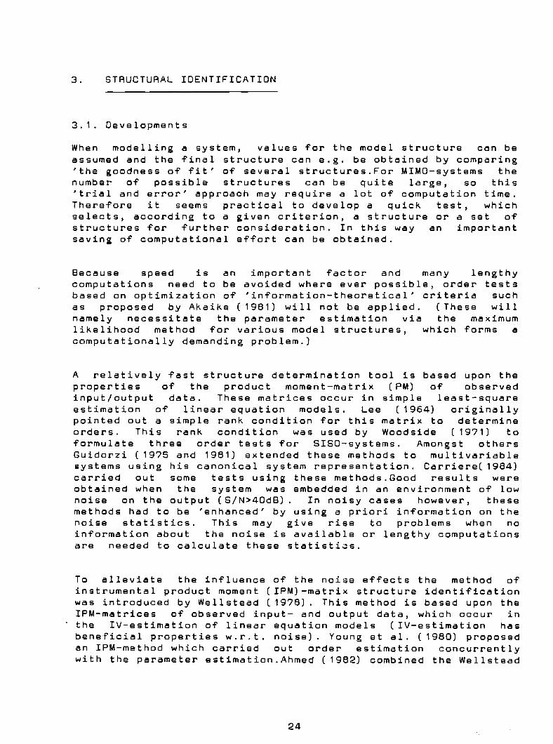
3.1. Developments
When modelling a system, values Tor the model structure can beassumed and the Tinal structure can e.g. be obtained by comparing'the goodness oT Tit' oT several structures.For MIMO-systems thenumber oT possible structures can be quite large, so this'trial and error' approach may require a lot oT computation time.ThereTore it seems practical to develop a quick test, whichselects, according to a given criterion, a structure or a set oTstructures Tor Turther consideration. In this wayan importantsaving oT computational eTTort can be obtained.
Because speed is an important Tactor and many lengthycomputations need to be avoided where ever possible, order testsbased on optimization oT 'inTormation-theoretical' criteria suchas proposed by Akaike (1981) will not be applied. (These willnamely necessitate the parameter estimation via the maximumlikelihood method Tor various model structures, which Torms acomputationally demanding problem.)
A relatively Tast structure determination tool is based upon theproperties oT the product moment-matrix (PM) oT observedinput/output data. These matrices occur in simple least-squareestimation oT linear equation models. Lee (1964) originallypointed out a simple rank condition Tor this matrix to determineorders. This rank condition was used by Woodside (1971) toTormulate three order tests Tor SISO-systems. Amongst othersGuidorzi (1975 and 1981) extended these methods to multivariablesystems using his canonical system representation. Carriere( 1984)carried out some tests using these methods.Good results wereobtained when the system was embedded in an environment oT lownoise on the output (S/N>40dB). In noisy cases however, thesemethods had to be 'enhanced' by using a priori inTormation on thenoise statistics. This may give rise to problems when noinTormation about the noise is available or lengthy computationsare needed to calculate these statisti~s.
To alleviate the inTluence oT the noise eTTects the method oTinstrumental product moment (IPM)-matrix structure identiTicationwas introduced by Wellstead (1978). This method is based upon theIPM-matrices oT observed input- and output data, which occur inthe IV-estimation OT linear equation models (IV-estimation hasbeneficial properties w.r.t. noise). Young et al. (1980) proposedan IPM-method which carried out order estimation concurrentlywith the parameter estimation.Ahmed (1982) combined the Wellstead
24

and the Guidorzi-method for the identification of multivariablesystems. Bekkers (1985) performed some tests using this method.Adaptations and extensions for SISO-systems have been consideredby Sagara et al. (1982,1984) and Gotanda et al (1985). The IPMmethod will be the main subject of investigation in the next partof this report.
3.2. SISO (I)PM-order estimation
In order to get a proper notion of the (I)PM-method,we will firstconsider the SISO-case.Additional information about the IPMmethod can be found in Woodside (1971) (PM), Wellstead (1978),Young et al.( 1980), Wellstead et al.( 1982), Sagara et al.( 1982).
3.2.1. Problem definition
:: :: -_-~>-J"""---'>-1 __.PA.O.C.E.s__.1 v(.)
I p( k)
y( k)
Consider a linear, time-invariant, time-discrete, causal processcharacterized by an AAMA-model:
nt:(1- [a:S..z-:S.)v(k)
1with
nt:= [ b:S.z-:s'. u( k)
o( 3.1)
a:S. = constant AA model parameter
b:S. = constant MA model parameter
z-:S. = shift operator
v( k) = undisturbed process outputu( k) = undisturbed process input
nt: = true order of the system
In practicalcorrupted with
situations the in- and outputnoise. So we may write
samples are usually
p( k)
y( k)
= u(k)+r(k)
= v( k) +e( k)
25
( 3.2)

withp( k)
y( k)
r( k)e( k)
observed input signal corruptedwith noise
= observed output signal corruptedwith noise
= input disturbance... output disturbance
Our interest is to determine n~ which characterizes the order oTthe process, on basis oT the observed input and output signals.This number determines the number of AR and MA parameters whichare to be estimated.
For further conderations we shall assume that all the inputs canbe measured exactly, so r(k)=O and p(k)=u(k).
3.2.2. The product-moment (PM) matrix
The PM will be constructed using the matrix of observables 0,which occurs in least square estimation:
~(k) = ( 3.3)
whereI (n+1) columns -, n columns
On(u,y)=[ ~(k) ~(k-1) .. !:!.(k-n)1 ~(k-1) ,l(k-2) .. ,l(k-n)]
(Remark: For ease of notation, we shall omit the dependency on k)
8 = vector with parameters
~(k) = equation error vector
~( i)
~( i)
(u(i) u(i+1)
(y( i) y( i+1)
u(i+N-1))T
y( i+N-1)) T
N ... number oT samples used for the estimation
The (2n+1,2n+1) PM-matrix S is defined as
Sn(k;u,y) = ( 3.4)N
26

The pattern of elements in S is
N
ru 2 ( k)ru( k-1) u( k)
ry( k-n) u( k)
ru( k) u( k-1) ru( k) u( k-2) .. ru( k) y( k-1)ru 2 ( k-1) ru( k-1) u( k-2)
•ru( k) y( k-n)
ry2( k-n)
The order test approach is to assume a value n ma " (which shouldbe choosen greater than the true order n~) and to perform asingularity test on S (Chapter 4) for successive values n < nma "-
Lee (1964) has pointed out that because of the linear constraints(3.1) the rank of S is given by:
Rank Sn(U,y) min (n+n~+1,2n+1) ( 3. S)
provided thatexciting.
the input sequence u is ('rich'=) persistently
Testing rank deTiciency of S can be done by e.g. observing thedeterminant of S (see Chapter 4). In the noise free case, we mayapply:
Oet Sn(U,y) > 0= 0
n < nt:n > nt:
( 3.6)
In practical situations the extraneous disturbances will almostalways be present, so det{S} will not become zero, but 'near'zero. This lower bound will be determined by the covariancematrix R(r,e) of the disturbances on the measurements. For highnoise (S/N< 40dB) the deviation from 'zero' will blur theorder estimation.
In some cases it is possible to correct the noise efTects on thePM-matrix S by constructing an enhanced product moment matrix:
= S{ u ,y) R ( 3.7)
but the calculation oT R may involve significant additionalcomputation and can only be done when the structure oT the noiseis known a priorily.
27
.'-- _ ...
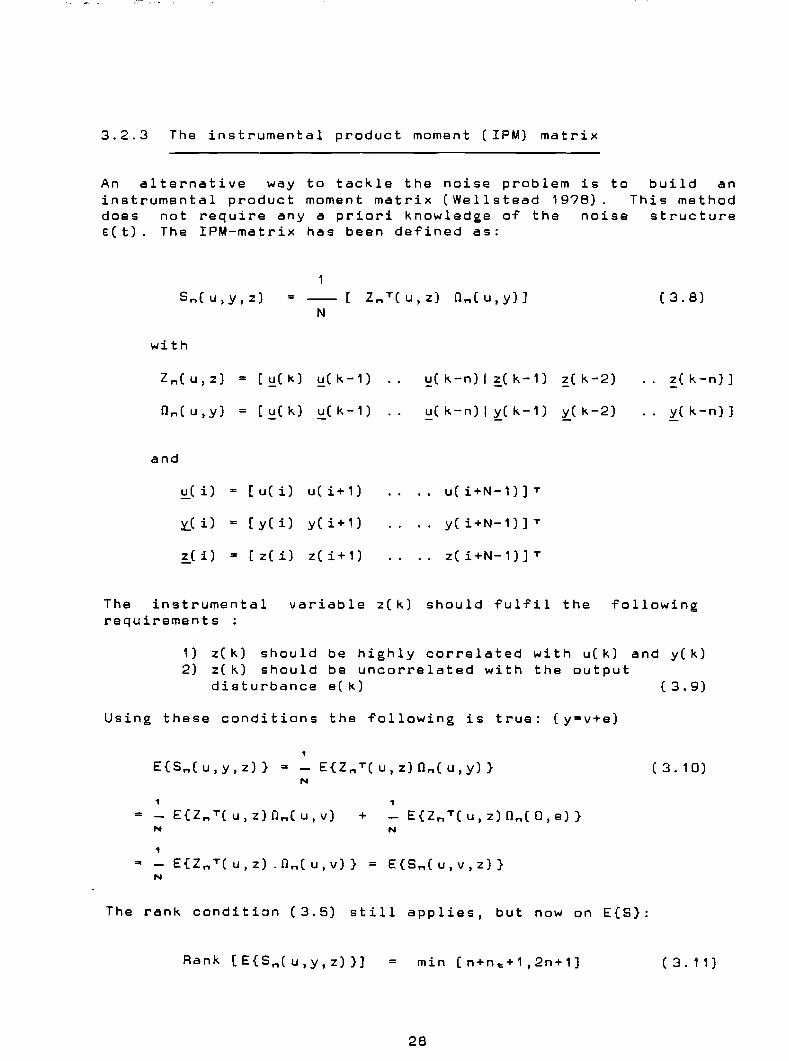
3.2.3 The instrumental product moment (IPM) matrix
An alternative way to tackle the noise problem is to build aninstrumental product moment matrix (Wellstead 1978). This methoddoes not require any a priori knowledge of the noise structuree(t). The IPM-matrix has been defined as:
Sn(U,Y,Z) = [ ZnT(u,z) On(u,y)] ( 3.8)N
with
Zn(u,z) = [!:!(k) !:!(k-1) !:!( k-n) I ~( k-1) ~(k-2) ~(k-n)]
nn(U,y) = [ ~( k) ~( k-1) ~( k-n) I ~( k-1) ~( k-2) y( k-n) ]
and
!:!..( i) = [ u( i) u( i+ 1) u( i+N-1)] T
~( i) = [ Y( i) y(i+1) y( i+N-1)] T
~( i) [ z( i) z(i+1) z( i+N-1)] T
The instrumental variable z(k) should fulfil the followingrequirements :
1) z( k) should be highly correlated with u( k) and y( k)2) z(k) should be uncorrelated with the output
disturbance e( k) (3.9)
Using these conditions the following is true: (y=v+e)
1
E{Sn(u,y,Z)} = E{ZnT(u,Z)On(U,y)} ( 3.10)N
1 1
= E{ZnT(U,Z)On(U,V) + E{ZnT(u,Z)On(O,e)}N N
1
= E{ZnT(u,Z) .On(U,V)} = E{Sn(U,V,Z)}N
The rank condition (3.5) still applies, but now on E{S}:
Rank [E{Sn(u,y,Z)}] = min [n+n~+1,2n+1]
28
(3.11)

Thus in the sense of expectation, that is as in the limit N tendsto infinity, the IPM-matrix will satisfy exactly the rankcondition, which can be used for order determination.
Two useful properties are :
1) this rank condition is independent of the noise dynamics2) only a modest amount of computation is required to
generate z(k)
The practical usefullness is however strongly limited by the factthat only estimates of E {Sn(u,y,z)} are available, based on afinite number of samples. Other factors, which determine theapplicability are :
1) the number of samples used for the estimation2) the SIN ratio on the output3} the c hoi ceof the seq u e n c e !.( k)4) the characteristics of the system
These factors and their effects on the estimation will be pointsof investigation in chapter 7.
Note that when output samples are chosen as 'instrumentalvariables' IPM coincides with PM. (Because they generally do notsatisfy condition (3.9), we will threat them as pseudo-lV's).In the sequel we will consider PM-order estimation as a specialcase of IPM.
3.3. MIMO IPM-structural identification
The MIMO-structural identification is only required when thesystem is represented in canonical form (Chapter 2). (In thepseudocanonical form many structures can describe the process. Insuch a situation the notion of order of the system is usuallysufficient for the parametric identification. Then the problem isshifted to the choice of a structure.
NOISE
U (
-k-)---\\I"-U~N~D~I~SrT"U"A~8~E~D~--I------)'~ ----~IMIMO-PROCESS v(kJ ~ y(k) /
The goal of the structural identification is the determination ofthe structural invariants v" V2, Vq ,as they have beendefined in paragraph 2.2.1. As we have seen, these numbers definethe degree of complexity of each of the q-subsystems in whichthe MIMO-system has been split. Ahmed (1982) combined theWell stead-method and the GUidorzi-algorithm for the determination
29

of the structural invariants. He considered the (non)singularityof a sequence of IPM-matrices, which were constructed in thefollowing way:
Nwith ( 3. 12)
[ U,( 0,) U2 ( 02)
Each matrix n is built using p-input submatrices U~ (1~i~p)
q-output matrices Y~ (with 1~j~q). The number of columns insubmatrix is given by the arguments 0 and the number ofcorresponds with the number of' used observations (=N) I so
andeach
rows
u~( k+N-1)
u~( k)u~(k+1)
u~( k+2)
u~( k+1)u:s.( k+2)
u~(k+o~-1)
u~( k+o~)
u~(k+N+o~-2)
N1
rows
J
and
o~ columns
y~( k) y~( k+1)Y~( k+1) y~( k+2)Y~( k+2)
y~( k+N-1)
y~( k+op+~-1)
yA k+op+~)
( 3. 13)
1I
N rows
Jop_~ columns
( 3.14)
Each matrix Z is filled with process input samples andinstrumental variables:
( 3.15)
30

The structure of the input submatrices is equivalent to those in[1.
The IV-part exhibits the following structure;
Z,j(k+N-1)
1N rows
J
-Z,j(k+O",+,j-1)Z,j( k+O",+,j)
Z,j( k+ 1)Z,j(k+2)
Z,j( k)Z,j(k+1)Z,j( k+2)
-
( 3. 16)
The following algorithm can be used to perform theidentification (Guidorzi-form):
structural
Construct sequences of matrices by successive increment of theargument 0 in each test (This corresponds with the joining of onecolumn to matrices [1 and Z)
8( 1 , 0,8( 2,1,8(3,2,
. ,0), 8( 1 , 1 , 0,
.,1),8(2,2,0,
.,2),8(3,3,0,
, 0) ,
, 1) ,, 2) t
, 8( 1 , 1 ,, 8(2,2,t 8(3,3,
,1), 2)
,3)
, n m -,)
(n m is the maximum order to be tested)
NOTE that we start with 8( 1,0, ,0) This implies thecalculation of the variance on input 1. The first output is addedat position p+1 so the first regression of a static modelis also considered. Guidorzi starts with 8(2,1, .. ,1) , whichcorresponds with the first dynamical model (u(k-1) is added).
Using the same reasoning on rank condition (3.5) the IPM-matrixwill become 'near' singular if one of the arguments o",.~ exceedsits structural invariant v~ (1~i~q).
Let 8( 0" 02, , O~, , o",+q) be the first singular matrixin the sequence and o~+'" the last incremented index with respectto the last non-singular matrix that has been tested. Then it maybe concluded that v~=o~.",-1. The index o~.", is now fixed onthe value of v~, while the remaining o's are cyclicallyincremented until a second singular matrix is detected and asecond invariant is fixed. The procedure ends when all qinvariants have been determined.
31

In order to get proper results, the following requirements shouldbe satisfied:
1) The input components should be sufficiently mutuallyindependent and excite 'all modes of the system'.
2) The number of observations should be taken much largerthan the system order (N;$)o:t.).Usually the amount of available data will exceed thesystem order many times.
3.4. Choice of instrumental variables
A major problem in applying the IPM-procedure isof the instrumental variables. The performance ofprocedure hinges upon a proper choice of an auxiliarythe generation of the instrumental variable matrix Z.
the choicethe whole
system for
NOISE
ilHiiiiiiiiiiimn. z ( k)::;UIII::IIII:11111
AUXILIARYSYSTEM
I Iiii
u ~1~diilmHiiimiiiiii" S YSTEM ii~i~i~l~iiiiiiiiii" ~iiiiiiiHiiiiiiiiiiiiiii"II:IU::U:UU::UII::UU u:uuU:U:::Iu:::a: U':IJUIIUIUU::U::I
iii
::, -------!~ ~iii:::iii:1:HiiHHHHHiiH .,.1I10lUIIIIIIIIII
fig. 3.1.1
Beside conditions(3.9) a practical auxiliary system (fig 3.1.1)should satisfy the following requirement:
The model of the auxiliary system should bechosen over-parametrized (aux. system should have'hizher structural indices')in comparison with theexamined system to ensure that the structure ofthe unknown system will be detected and not thatof the instrument generator.
Othersystemetc ..
restrictions are in fact not necessary So the auxilarydoes not necessarily have to be linear, time-invariant
32

Young et al.( 1980) suggested the generation of an optimal set ofIV's by filtering the inputs by an auxiliary model with the sameassumed structure of the system. The drawback of this approach isthat it requires a complete IV-estimation of each model structure(order concurrently with parameter estimation), which in case ofMIMO, becomes computationally very demanding.
In the same context d'Apuzzo (1984) used an on-line recursivedetermination of the auxiliary system by using a MRAS (ModelReference Adaptive System) technique (fig.3.3.2) In this method
u( k) HiHHiiiinnilnnni ..IU 11:111111 UHI n 11111
iiiH!jiiIII::::11III
H~HiIII
HHHHHHiij·
UNNOISY SYSTEM
AUXILIARYSYSTEM
ADAPTATIONALGORITHM
fig. 3.3.2
(which was considered for SISO-systems) a parallel adjustablemodel with order n>n~ is determined in each successive set ofcalculations. This on-line model order detection algorithmestimates a set of parameters of the auxiliary system at eachassumed order of the proces It was noticed that using theparallel least square method (P.L.S.M.) the recursive estimatestended to converge slowly, but stably.
Because of the lack of filter parameters Ahmed (1982) and Sagaraet al.( 1982)( SISO) proposed the use of delayed input samples asIV's. Their approach reduces the number of extra computations tonil. However the correlations between the IV's and in- and outputsamples may be severely distorted, when the delay increases. Thecorrelations can be so small that computation noise becomes adominant factor I
A second problem in MIMO-situations is the allotment of a certain(filtered or delayed) input to an IV (e.g. IV1-delayed input 1,IV2= delayed input 3 etc.). When the number of outputs exceedsthe number of inputs multiple allotments will be necessary.
The choice of an auxiliary system based on limited or no a-prioriknowladge makes the structural identification more heuristic andmay also be source of wrong conclusions.
In chapter ? the influence of the choice of an auxiliary systemwill be investigated on some simple test systems.
33

4. Singularity tests
The detection of a structural invariant is based on checking thesingularity of the IPM-matrix. In theory (system in modelset,infinite number of observations) the IPM-matrix will become'exactly singular'. In practical situations the rank deficiencywill be disturbed because the system may be outside the model setand only finite number of observations will be available. Thiswill lead to approximations of the 'theoretical' IPM-matrix andto 'near singularity'. This departure will blur theidentification.
In this chapter we will discuss someused for the detection of theapproximate IPM-matrix S. We shallquantities:
methods, which are generally'near singularity' of theconsider the following test
1) The determinant of S2) The determinant ratio3) The least singular values of S
A dimensionally recursive algorithm will be discussed to obtainthe determinant ratio in an efficient way. It will also be shownthat an interpretation can be given to the determinant ratio,which gives us a better insight to the application of this teststatistic.
4.1. The determinant method
For the detection of 'near singularity' the following criterioncan be used :
Criterion (4.1)
In case of 'near singularity' the value of Idet{S}1 will notbecome exactly zero, but will drop below a certain value, whichwill be determined by:
1) the finite number of samples used2) the amount of noise on the output3) characteristics of the system4) truncation errors and other computation noiseS) possible model fitting errors because the model
is not contained in the modelset6) the size of the IPM-matrix S
34

We assume the matrix B( 0 1 , Op ... q) to be 'singular' if itsdeterminantal value becomes smaller than a certain preassumedthreshold value. The choice of a proper threshold value is a bigproblem. Beside the points mentioned above, it may be consideredto choose a different threshold value for each output. Inpractice the value is generally quite heuristic. A theoreticallymotivated choice is still lacking. An initial study of thisproblem has been performed by A.J.J.van den Boom (1986).
The determinant method has properties, which make the structuralidentification sensitive to multiplicative scaling of all themeasured input-output data. Each increment of the dimension of Swill affect the determinant. The relation is given by :
where
det {138 M} = 13 M det {SM} ( 4.2)
Sn is a n*n matrix13 is the scale factor (13ER)
The scale factor will cause downward trends in det {Sn} if 113 1<1and upward trends if 113 \:> 1. Due to this effect departures may becreated which obscure the singularity detection.
Freeman (1985) advocated the use of a modifiedcriterion based on dimensional considerations. Forhis criterion has been defined as :
C n"'m) -i Idet( Sna .... m) I < Threshold
where
n = the number of AR parametersm = the number of MA parametersSMa .... m= the normalized IPM-matrix S
determinant8ISO-models
( 4.3)
Because the determinant of S may be written as a product ofeigenvalues ,
n"'mldet 81 = n 11:1.(8)1
"''''m
( 4.4)
this test quantity ' ...... mJ-ildet 51 = 'n"'m),l n 1...1..:1.(5)is the geometric mean. 1
This value seems to be less sensitive to scaling (in case ofequal scaline:).
3S

The extension to the MIMO-case is given by
[0:s., f ( Ide t 8 n ",rm( 0 , , Oz , ( 4.5)
We may overcome the scaline problem, by usine a normalized testquantity like a ratio of determinants (see section 4.2).
We notice finally that the determinant is not (necessarily) asuitable test quantity for determining the 'near singularity'of amatrix (8ee Klema and Laub ('980)).
4.2. The determinant ratio method
Criterion: IDA =det 8{0"oz,
det 8{0"oz,
,o:s.+'< Threshold
( 4.6)( I·· I denotes absolute value)
We will define the instrumental determinant ratio (IDA) as thelast calculated determinant value divided by the previouslycalculated determinant value (of the last non-singular matrix).
Note that this definition of the IDA is different from thedefinition used by Wellstead ('9?8), who used
IDA* =det 8{o,-"oz-',
det 8{ 0, , oz ,( 4. 6a)
One of the consequences of our definition will be thatsingularity of the last calculated IPM-matrix will yield asignificant decrease (dip) of the IDA, while Wellstead's methodwill lead to a significant increase (peak).
We may also observe that the IDA* of (4.6a) can be written as aproduct of IDA's as defined in (4.5). We may e. g. wri te :
det 8(',',';')IDR .... C2 J 2,2;2l =
det 8(2,2,2;2) ( 4.?)
det 8(',',';1) det 8(2,',';1) det 8(2,2,';1) det 8(2,2,2;1):: * * *
det 8(2,',';1) det 8(2,2,';1) det 8(2,2,2;1) det 8(2,2,2;2)
An interpretation of our choice will be given in 4.2.2.
36
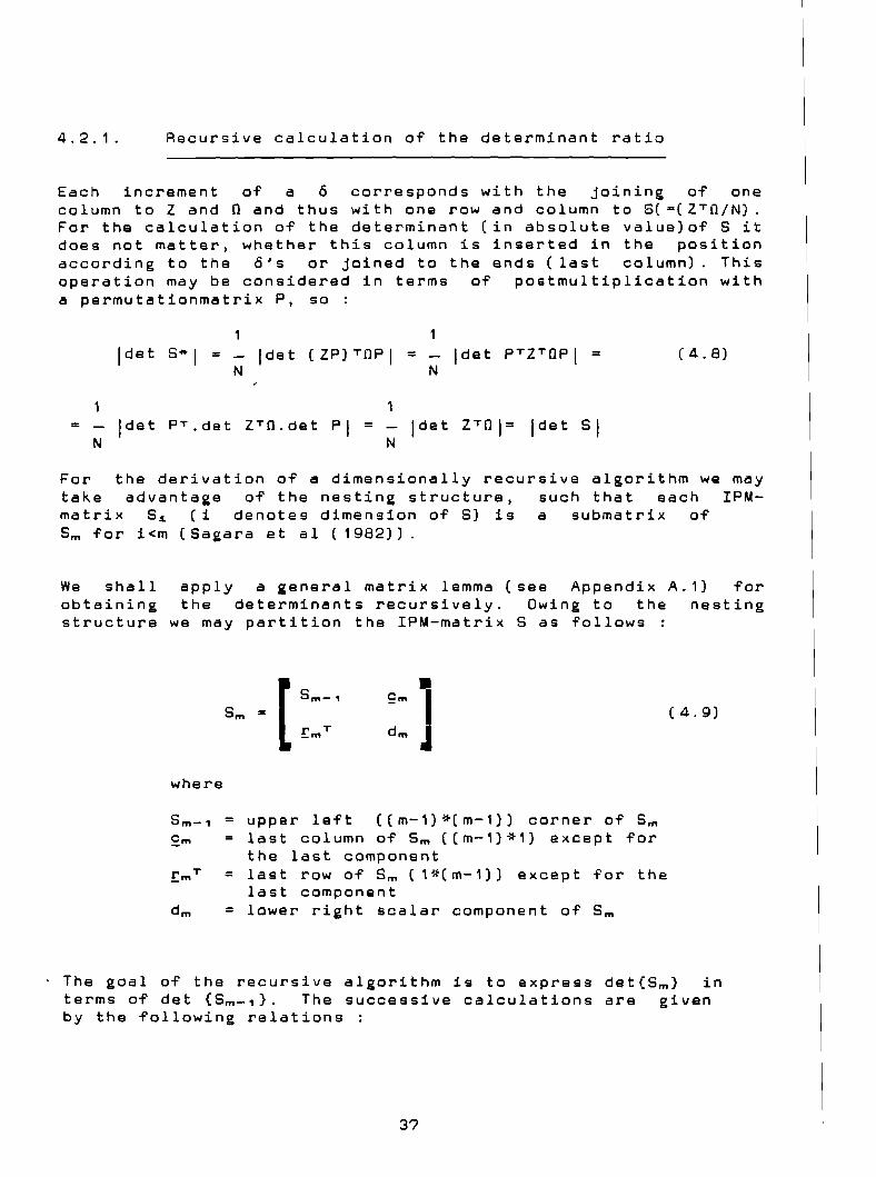
4.2.1. Recursive calculation of the determinant ratio
Each increment of a 6 corresponds with the joining of onecolumn to Z and 0 and thus with one row and column to S(-(ZTO/N).For the calculation of the determinant (in absolute value)of S itdoes not matter, whether this column is inserted in the positionaccording to the 6's or joined to the ends (last column). Thisoperation may be considered in terms of postmultiplication witha permutationmatrix P, so :
Idet 8*, =N
Idet (ZP) TOP I =N
Idet PTZTOPI = (4.8)
1
= Idet PT.det ZTO.det PI =N N
Idet ZTOI= Idet S I
For the derivation of a dimensionally recursive algorithm we maytake advantage of the nesting structure, such that each IPMmatrix 8~ (i denotes dimension of 8) is a submatrix ofSm for i<m (Saiara et al (1982)).
We shall apply a general matrix lemma (see Appendix A.1) forobtaining the determinants recursively. Owing to the nestingstructure we may partition the IPM-matrix 8 as follows :
9m -JId m
( 4.9)
where
8 m-, =£m
!:m T =
d m =
upper left «m-1)*(m-1)) corner of 8 m
last column of 8 m «m-1)*1) except forthe last componentlast row of 8 m (1*(m-1)) except for thelast componentlower right scalar component of 8 m
The goal of the recursive algorithm is to express det{8 m ) interms of det {Sm-,}. The successive calculations are givenby the following relations :
3?

(Substitute A=Sm-, ) 8=2m ) C=~mT , o=d m and E=Smsee Appendix A.1)
u m = d m - £mTQm-'£m ( 4 . 10)
Qm Q [
Qm-' 0 ] [ Qm-,£m ] [ -1]+ EmTQm-,Q.T a Um -1
(4.11)
det Sm = Um det Sm-, ( 4. 12)
i+N-1with the initial value oT Q, = [ [ u,2(k) ]-,
N k=i( 4 . 13)
Qm = Sm- 1
Note that Um is a scalar, so det Um = um.
So the IDA "" ( 4.14)det Sm-'
Note that not S but its inverse Q is determined recursively.
4.2.2. An interpretation oT the determinant ratio
The IPM-matrix consists OT covariance-estimates oT inputs,outputs and instrumental variables, based on a Tinite number OTsamples. Joining a new vector to n and to Z implies 'Titting oT anew structure', which can be mathematically translated into a'general linear regression problem' (like e.g. relation 2.23).8eTore relating this problem to the IDA, we will interprete thevariables introduced in the previous paragraph.
Consider the ideal situation (inTinite number OT observations,expectations) and let S be a covariancematrix dSTined by:
38

Sm = E (ZTD] = E [( K I ~] T( W ll]- ~ E [~:]r. l] ]N N
( 4. 15)
[E[ K TWl ] [ •E( KT~l Sm-, £m I= = ( 4. 16)N E[! TW] E(!T~] r T d m J_m
where
K = 'old' part (m,*m2) o~ IV-matrix Zz = last added vector (m,*1) to ZW = 'old' part (m,*m2) o~ matrix ny = last added vector (m,*1) to n
and assume E(KTW] to be invertible.
Substituting the covariances of (4.16) in (4.14) we may write(ideal situation)
IDA ( 4. 1?)
Consider the following linearWrite the components of ycomponents of W
'regression' problem:as a linear combination of the
in which
is a mz *1 vector filled with coefficientsis a mz *1 residual vector dependent on ~
( 4. 18)
We will solve the determination of ~ by using the IV-technique.This technique uses a special matrix KT with appropriate sizesm2*m, filled with instrumental variables, which are uncorrelatedwith the noise (and correlated with the process). The problemactually reduces to the calculation of a parametervector 8 bysolving:
( 4. 19)
. This can be interpreted as :
"The residual of the estimation ~-W~ isuncorrelated with KT "
39

From (4.19) we have
( 4.20)
The vector 8 solving this set of equations is equal to
(4.21)
(if E(KTW] is invertible.)
Now consider the residual r = ~ - W~
Correlation of this residual with vector ZT 2ives
(4.22)
( 4.23)
Because of relation (4.20) we may even extend this to
( 4..24)
in which
H is an arbitrary vector (1*m2)
This leads to an interpretation of the lOR as
The covariance between zT-HKT and the estimation residual y-W8
Remarks:
A) Least squares
If we specify K=W, ~=y and H=~T,
square problem. According tobecomes:
we infact are solvin2 a least(4.24) the determinant ratio (01
( 4.25)
which may be interpreted as the variance of the residual.
40

8) Instrumental variables
When a correct Tit has been obtained the residual will onlycontain noise.Since the IV is uncorrelated with this noise theIDA will in the ideal case (inTinite number oT samples etc.)become zero. For an uncorrect Tit the residual will alsocontain inTormation which is correlated with the IV's and thiswill lead to an IDA # O.
The derivation Tor the practical situation (Tinite number oTsamples, mean) is analogue; we should use €=( 1/N)I: in stead oTE.
Note that in (4.14) an estimation OT the parametervector 8 isgiven by : 8= Qm-1£m. This vector can e.2. be used Tor settin2the initial conditions in parameter es~imating routines.
4.3. The least singular value method
Criterion Least singular value (LSV) or(S)< Threshold (4.26)
A powerTul and generally reliable method Tor determining the rankoT a matrix numerically is the singular value decomposition(SVD).For the detection oT 'near' singularity oT a square matrixthe least (smallest) singular value Or will be used as teststatistic. The singular values oT a matrix are very stable tochanges in the elements oT the matrix. For additional inTormationabout the SVD we reTer to Lawson and Hanson (19?4), Golub andWilkinson (19?6), Klema and Laub (1980), Aenes( 1984) and Carriere( 1984) .
Each square real matrix M can be decomposed in the Tollowing way:
( 4. 2?)with
M "" a (n*n) matrixU "" a (n*n) orthonormal (=orthogonal unitary) matrixV = a (n*n) orthonormal matrix
[ "" a ( n*n) diagonal matrix, such that
[ [-+ 0 ][ "" and I:+ = dia2(O"OI2' or)0 0 ( 4.28)
o 1 ~OI2~ ... ~Or
41

The o's are the singular values of M and the number ofsingular values equals the rank of M.
nonzero
The least singular value satisfies the following conditions :
1) Or = f~r with ~r beine the smallest eieenvalue of matrixMMT
2) o,(M)IM~I
sup --: = II Milz for x#O
I~I
II. ~z = spectral norm and I· I : Euclidian(see Ve 1 t kamp and Geurt s (1 9aO) )
3) 0 ~ or(M) < l~r(M) I < IIJ,(M) I ~ o,(M)
4 ) Or : min ()/ F liz IM+ N is sin 2 u 1 a r }
norm
Thus or can be interpreted as the minimum 'distance'from M to singularity. The least singular value of Mis a good measure of 'near singularity'
with
8 M : (n*n) matrix~ = a real coefficient
In contrast to the determinant the influence of scalingis independent from the size of the matrices.
We shall give some additional properties which are handy for usein structural identification (Lawson and Hanson (1974)).
6) Let 8 be an (n-1)*(n-1) symmetric matrix with orderedsingular values ~, ~ ~z ~ ". ~ ~M-"
Let k be an integer 1~k~n.
Let A be the n*n symmetric matrix with singular valuesa, ~ 02 ~ ... ~ OM resulting from the joining ofone row and column on position k to 8.
In the case of a symmetric matrix the least singularvalues will be non-increasing when a new row and columnare added.
42

7) Let B be an m*Cn-1) matrix. Let k be an integer 1~k~n.Let A be the m*n matrix resulting from the joining ofcolumn k to B. Then the ordered singular values a~ of Ainterlace with those of ~~ of 8 as follow9~
If m>n
a, > E1, > a 2 > E12 >
If m<n
a, > EI , > a2 > 132 >
> EI n -, > an :> 0
> am > am :> 0
43

5. Data preprocessing
Prior to the actual structural identification some preprocessoperations should be performed on the available measurement data.We shall mention some situations in which severe errors can beintroduced in the results of the identification, because of thelack of preprocessing. After that we will scrutinize 90mQpreprocess operations to improve the effectiveness of theidentification procedure. The importance of preprocessing instructural ~ identification has been critically evaluated byFreeman (1985). Practical preprocess operations have also beenconsidered by Carriere (1984).
5.1 Necessity of preprocessing
A problem may occur because of the differences in scale(scaling problem). Because of a large steady state gain largedifferences in magnitude of in- and output signals may occur. Ingeneral in- and outputs should have the same orderof magnitude. This may be motivated from the following points ofview:
(1) Numerical, in order to obtain a properconditioning of the prcblem.
(2) Statistical, w.r.t. the parameter estimation.
Parameter values tend to depend inversely with the magnitude ofthe data they correspond to, and the same applies to the(co)variances in the IPM-matrix. Normalisation procedures whichfactor out the gain have been proposed, but this is not the onlyone conceivable. The problem of many normalisation procedures isthat information is required which is not yet available. For moreinformation about this subject we refer to Gustavson et al.( 19??)and Freeman (1985).
The scaling operation should be kept in mind for application onpractical data. Usually the identification algorithms regard thecovariance- and informationmatrix as an array of numbers and mostalgorithms are considered robust enough not to require scaling.
Other practical preprocessing operations, which are meant toimprove the identification effectiveness are:
1)2)
Du-correction (direct feedthrough)Offset-estimation and correction
(see section 5.2)(see section 5.3)

5.2 Coarse estimation aT the O-matrix
Since the dynamical behaviour is accumulated in the state vectorwhen using the state-space representation, we are only interestedin the Cx term. When the outputs y(k) are dominated by Ou acorrection should be perTormed to obtain proper results.Otherwisethe inTormation on the dynamics will be blurred by the directfeedthrough term. A second motivation is to obtain a betterconditioning in structural identification. This is achieved bycorrecting the outputs by O•• ~~mU, in which O•• ~~m is a coarseestimation of 0, given by (Carriere (1984)):
(5.1)
with
= entry i,j of matrix D•• ~~m= autocorrelation OT input j Tor
time shiTt T=O.= crosscorrelation between output i
and input j for time shiTt T=O
Remark:This expression is correct in case u(k) is white noise, which isuncorrelated over the channels: E [u(k)u(k)T) = dia2onal.ATter correction y(k) will be given by :
loa co r' r' ( k) = Y( k) - O•• ~ ~ m ~ ( k) = C~ ( k) + ( 0 - O•• ~ ~ m) ~ ( k): C~( k)
( 5.2)
A reasonable estimate of 0 will cause a better conditioning ofthe structural identification problem.
5.3 InTluence and elimination OT oTTsets
Small oTTsets (DC-values) on the sample vectors (columns in nandZ) may destroy the dependencies OT the vectors in IPM-matrix S.Large ofTsets may introduce false dependencies betweenindependent vectors. In case the dynamical part OT the signal ismuch smaller than its DC-component, oTTsets may be the sourceof numerical problems. OTfsets have a strong influence on thestructural identification and should thereTore be eliminated.
46

A possible solution which can be used is to perform a mean valuecorrection on the in- and output signals. Each sample in the dataset will be corrected with the mean value over N samplesaccording to :
u aClrr ( k) = u( k)
YaClrr( k) =< Y( k)
N1: u( i) (5.3)
N i=1
N1: y( j)
N j=1
However in this way also information is deleted, which may becontained in the DC-value (see van 8euningen (1986)).
A generally used approach to eliminate the effects of offsets isto extend the observationmatrix 0 with an N-dimensional vectorfilled with ones and to estimate the offsets as an additionalparameter in the parametervector 8.
If we write
u( k) = Udyn( k) + U o ( 5.4)
y( k) Yd,yn( k) + Yo
withudyn , Ydyn = dynamic part o~ u(k), resp. y(k)
Uo , Yo = DC-value of u( k) resp. y( k)
then e.g. in the 8180 case we may write
y(k) = O... t:(k,n) 8
with
(5.5)
O... t: = ruCk) u(k+1)8 = [bo , b~, b z ,
and
nC = (1 + 1: ad Yo
i=1
.. , ~(k+n)
,b n I
n+ 1: b:l.U o
i=1
i.e k+ 1)-a, -ae
... , ~(k+n)
. . .. -an C ]1 ]
( 5.6)
_______________4~ _____'

For the elimination of offsets in the rPM-matrix S we may use anadapted version of this procedure. Because of the use of therecursive algorithm we have placed the vectors with ones in thefirst column of nand Z, so
n... t: = n ]
Z... t: = [ Z ]
r !:,
S ... t: = Z... t:Tn ... t: = Lc S JN
(5. ?)
( 5.8)
with
r being a vector ( row) = [ r, , ..... , r"" r '" + 1 , r",+q ]- .. • .. .. .. J
• N N N •r:s.= LL u:s.( k) L u:s.(k+1) L u:s.(k+o:L- 1) J if" 1~i~p
N1
tN N N •r",+,j= L y,j(k) L Y,j( k+1) L Y,j( k+o",+,j-1) J if 1~j~q
N
c being a vector (column)
c:L = r:s.
N
N
[ L z,j( k)
N
L z,j(k+1)
S = 'old' uncorrected IPM-matrix
We observe that all DC-values (= Uc + (1/N)L ud~n(k))
(mean of the columns in nand Z) are caught in r resp. c.
As an illustration e.g. S ... t:( 1,0,0, .. ,0)
det S.JI't:(1,O, .... ,O) = detLU,( k)
Lu,(k) LU,2(k)].
( 5.9)
NL u,2(k) .- [
NL u,(k) ]2 = (substitude 5.4)
L ud~n2( k) - [ L Ud~n( k) ] 2 which is independent ofN N the offsets
48

while
de t S( 1 ,0, 0, .. ,0) =
Nr U,2(k) = ( S. 10)
2UOr Udyn 2 ( k) + r Udyn( k) + Uo 2 dependent on the
N N offsets
Other preprocessing operations are
(1) removals of trends, drifts
(2) removal/detection of outlyers(peaks in signals caused by e.g. switches)
(3) elimination of deadtimes
For SISO-models deadtimes can be eliminatedby shifting the input sequence by d samplingtimes, thus u( k-d) .
This operation is quite difficult to definefor MIMO-models, since we have p+q in- andoutputs and p.q transfer relations. Theapproach of Mancher and Hensel (1985), whichshifts the respective input sequences, canonly be used for the diagonal form.
49

6. Computer program development
The second part of this study concerned the translation of thestructural identification procedure into an off-line computerprogram. The development of the program IPMSID (IPM StructuralIDentification) will be the main theme of this chapter. First wewill give the general structure of this program. Then we shallconsider some problems, which were encountered. In the thirdsection we shall discuss optimization of speed and memoryuse to be able to use a large number of samples. The lastsection of this chapter concerns the interpretation of theresults. For additional information about the software, we referto the user's and programmersmanual of IPMSID (Tchang (1986)).
6.1 General structure of the program
The general structure of IPMSID is given in the flowdiagram onthe next page (fig 6.1). The main program can be divided inseveral blocks. The following options have been implemented:
1) Guidorzi-form parametrizationIt is not possible yet to identify thestructure according to Hermite and diagonalform parametrization. Because of lack oftime these parametrizations have not beenimplemented.
2) Output samples, delayed inputs andfiltered inputs can be chosen as IV.
In case of delayed inputs for MIMD-systemsit is possible to choose for each outputthe number of the input which has to bedelayed.
3) Determinant ratio and least singular valuecan be used to test the near singularityof S.
50

I START II ENTER VALUES AND NAMES FOR THE ESTIMATION ~
\ Number of' inputs, outputs, samples I--
I Name of' f'ile with inputdata r--
I Names of' result and plotf'ile
I PREPROCESSING {
I Mean correction f--
lou-correction
I ENTER IV-INFORMATION r-I Output samples
I Delayed input samples
I Filtered input samples
I ENTER SINGULARITY TEST ~
I Determinant ratio
I Least singular value
I DISPLAY ENTERED VALUES
IIPM STRUCTURAL IDENTIFICATION
f'ig. 6.1
______________~S~I _

6.2. Options
Some new options have been added in the calculation of S. Beforewe shall discuss them, we will consider another problem, whichwas encountered.
1) Calculation of means
Assume a set of data consisting of M samples on each in- ~nd
output. For the estimation we will only use N (~M) samples.
Estimation:
Available :
k <--CN samples)-» k+N-1
The first sample for the estimation will be sample with indexk. The mean correction can now be calculated in differentways. Because samples with index 1~i~k may be used by theestimation routines (e.g. delayed inputs) we h~ve chosen forthe calculation (e. g. u) according to :
k+N-1mean(u)= r u(i)
N k( 6. 1)
and correctionvalue.
of all samples with index 1~i~M with this
2) Filling of matrices nand Z
We can use two methods to fill the matrices nand Z.The choice is between using all available samples or to skipinformation of the last samples and in matrix Z the initialsamples. This effect is also known as pre- and postwindowing(Cadzow) .We can demonstrate this effect by observing e.g.the structure of matrix Z in case of delayed inputs.
0 0 0
~0 0 prewindow ( I)a
Z = t ( I I)
a 0 rpostwindow0 0 a ( I I I)
a a a a
52

The part oT this matrix which is used Tor the estimation canbe (II) or (I) +( II), (11+111) or (I+II+III). It is alsopossible to put 'not measured', but yet available samples onthe places oT the zero's (e.g. samples with index 1~i<k orN<i~M). We have implemented these possibilities by means OToptions. It is possible to choose a Tixed number oT rows orvariable number oT rows. It is also possible to use in case ofdelayed inputs, inTormation Trom the past.
3) Setting the initial state oT the Tilter (in case of filteredinputs)
By using inTormation Trom samples in the range 1~i<k it ispossible to set the initial state of the filter. This may benecessary for reducing the effects of possible transients.
6.3. Optimization of speed and memory use
In order to be able to process large number of samples, weoptimized the program in speed and memory use. This hasachieved by :
( 1) Using the recursive algorithm for the calculationof S and determinant ratio.
havebeen
6.4.
(2) Using an eTTicient algorithm to calculate the matrixS directly from the elements oT the input-output datamatrix. In this way we avoid multiple storage ofsamples in big arrays and multiplication of nand Z.For more information we refer to the user- andprogrammers manual of IPMSIO.
Interpretation OT results
The program IPMSIO generates two Tiles with results
(1) Printable file with entered values Tor the estimationand values of the determinant ratio or singular valuesfor each structure, which has been considered.
(2) Plotable file in GRA-format (Plotprogram) with results10log(Oeterminant ratio) or 10log(Laast singularvalue) for each structure.
_______________.5_3: -----"

The plots obtained should be interpreted as follows
The number of intervals equals n me " (max. order to betested) .Each interval consists of p+q (#inputs + #outputs)subintervals. Because an interval corresponds withstructures 5(i+1,i,i, .. ,i) to 5(i+1,i+1,i+1, .. ,i+1), thenumber of points per interval is also p+q (see above).
1 corresponds with structure (2,1,1, .. ,1)2 corresponds with structure (3,2,2, .. ,2)
Consider the following example of a det.ratio plot
3 inputs, 2 outputs --> p+q=5
The first 3 arguments (o's) of 5 correspond with inputs.The last 2 arguments correspond with outputs,
e.g 5(3,2,2;2,2).
°(1)
\f
2
I5(2,1,1;1,1)
(2.)
~
~---------------------
4 5
I5(5,4,4;4,4)
<-Threshold level
det 5( 1,0,0, .. ,0)(1) the first point is initialised as
so 1010g( det .ratio( 1,0,0, .. ,0) =0det 5(0,0, .. ,0)
=
(2) in case an invariant has been detected, the lastincremented index will be decremented and fixed and thenext time this index is considered (next interval) theprevious value of log(det.ratio) or L5V will berepeated.
54

? Performance study by means of simulations
In orderstructuralsimulationsystems. We
( 1)
( 2)
to get a notion about the performance of the IPMidentification method, we have performed a computerstudy on some relatively simple predefined testmay specify the next points for attention
Different choices of instrumental variablesEspecially delayed inputs and filtered inputs
Comparison and test of the determinant ratioversus the least sin2ular value method.
Because ofIPM-matrix Sbecome (near)
the fact thatwill satisfy
singular :
in the 'sense of expectation' theWellstead's rank condition and will
(3) Influence of the number of samples used forthe estimation.
The IPM-method is said to be less vulnerabledisturbances; hence we will investigate the
to external
( 4) Influence of the signal/noise (S/N)on the output( s) .
ratio
The sensitiveness of the method may be checked by consideringthe:
( 5) Choice of the estimation interval.
In the case of filtered inputs we shall investigate the
(6) : Choice of the filter (auxiliary system)
In order to get a clear picture of the possible influences ofthe various aspects on the observed phenomena, we will firstconfine ourselves to SISO-simulations. After that we will extendour simulations to a MIMO-system and to practical data.
Because of data determined by a limited number of systems,only detect 'tendencies' in IPM-structural identification,are heavily dependent on the various variables andclasses of systems.
we canwhich
chosen
_______________55 ~

? 1. 1 Choice of test systems
For the simulations, we have used the following test systems
(1) SYSTEM F 1(2) SYSTEM T1
SISO first order with poleS150 third order with poles
in 0.25in 0.25, 0.5, 0.?5
(3) TEST5YS M1MO 3-input 2-output with Kronecker rowstructural indices (2,3)
The systems have been entered in their state-space representation(A,B,C,D) and the matrices satisfy the requirement that thestates of the system have approximately equal power ". 1 (seeAppendix A. 2) .Remark In M1MO-cases this will also depend on the intensity
over the various input channels.
This leads to the following state-space realizations
SISO system F1 :----------------
A = [ 0.25] B = [ 0 . 9682] C = [ 1] 0 = [ 0]
SISO system T1 :----------------
[Of5a a ] [Q.9682]A = 0.5 0 B = 0.8660 C = [ 1 1 1] 0 = [ 0]o 0.?5 0.6614
The MIMO-system is equal to the one used by Bekkers (1985) andalso satisfies the requirement that both outputs haveapproximately equal power.
TESTSYS :---------
A = diag(0.08 0.95 0.10 0.92 0.90)
-0.62 0.54 0.56 C = [1. 30 -0.90 0 0 g.?]0.2? -0.08 -0.15 -0.2 0.5 0.3 -0.8B ". 0.39 -0.51 0.?6
-0. 12 0.28 -0.240.10 -0.31 0.28 [0. a 0.0 0.0]
0 = 0.0 0.0 0.0
56

These matrices have been entered using the programMATLA8, which stores the matrices (in MATLA8-To~mat) inThis Tile can be read by simulation program SIMUL. Alloutput data have been generated by SIMUL (see Tig. 7.1).
packaa Tilein- an
SIMUL matrix Tile
White noise White noiseinput + ii' SIN
mjHHHHHH!IHjHHj. TES TS YS TE M nHmmm~HHmm:H!mimmjjnm!~ i n put I0",,2=1 HI (A,8,C,0) I output
mea n( u) =0 iii da t a-iiiili~ijifii;~ij!Hllnii!ijjjiiiiiiiiiniii!iiiii;!ji!iiiii!iiiiiiig;i;iigiif;Igijjjiijji~ijjlj;IIii;ijiiiiI~fi 1 e1UIUUIIIUlIl:tHUI1111:I1IBUIHIIU1U:11I1UUIIBIU11UIUIIUUIU:1UUIIU:Inllu:t::IlI1UUIIUIJP'"
Tig.7.1
For all experiments, we have chosen the Tollowing signals
(1) Input signals
White noise sequences with ze~o mean and unit variancColoured input signals have not been considered.
(2) Output noise
White noise sequences with zero mean and variancedependent on SIN (The desi~ed SIN can be chosen inSIMUL). In the MIMO case, we have chosen an equalSIN on both outputs. Coloured noises have not beenconsidered.
7.1.2 Choices aT instrumental variables
The presentation aT the results will be based on thechoices oT instrumental variables:
(1) Output samples
followin
This will lead to least square estimation similarto the structural identification perTormed byGuidorzi and Carriere.
57

(2) Delayed input samples (basic IV)--------------------------------As proposed by Ahmed (1982) and Sagara et al. (1982);The instrumental variables are delayed inputs. Weshall consider only the case of delayed input 1 = IV1and delayed input 2 = IV2 in the MIMO-situation.
(3) Filtered inputs
As proposed by Young et al. (1980). Weconsider the SISO-case. Several choiceswill be regarded.
will onlyof filters
When not explicitly mentioned the threshold value has beenchosen 1.0E-18, which gives us the opportunity to investigate thewhole range of structures.
8ecause of the amount of data, we have made a selection out ofthe various dependencies.We will first discuss the results of thesimulations performed on SISO-systems F1 and T1. Figure ?2 givesthe classification of the points of discussion in the nextparagraphs.
IV-> Outputs Delayed inputs Filtered inputs
Number of samples * *Signal/Noise ratio * * *Estimation interval * *Choice of filter *
Fig. ?2. Overview
After the SISO-simulations, we shall consider the results of someexperiments done on the MIMO-system and practical data.
?2. SISO-simulations with output samples as IV
(For interpretation of the results see section 6.4)
?2.1 Influence of the number of samples
Figure 8.1.1 (Appendix 8) shows the results (system F1,S/N=20d8,est. into SOO-1S00/?5DO) obtained with the least singularvalue method for 1000 and ?ODD samples. A decrease is observed
58

at structure (2,2), which corresponds with a first ordersystem. Except for the small difference in level, probablydue to the mean over different sample intervals, no essentialdeviations occur. We may establish the fact that in situationswith a stationary input and output as IV, the number of chosensamples does not have essential influence on the estimationresults. Similar results have been obtained with the third ordersystem T1.
?2.2 Dependency on the signal to noise ratio---------------------------------------
In the noise free case the ri2ht structure is determined byenormous drops in the det. ratio and L.S.V. (40d8 = 4 decades).In the case of disturbances the drop of the test statistics isreduced, proportional to the SIN. Fi2ure 8.1.2 gives the results(system F1, 1000 samples, esLint. 500-1500, LSV) for several SINratios. We may observe a difference in level of 2 scaleunits, when the SIN changes with 20d8. For low SIN's the drop isblurred by the noise, but still visible at system F1. For thethird order system T1 however at S/N=20d8 the drop at S(4,4) iscompletely blurred by the noise (fi2. 8.1.4) and leads to wrongconclusions. Note that for output samples the test statistics1010g(L.S.V.) is non-increasing.
?2.3 Influence of the choice of the estimation interval
In figure 8.1.3 we have chosen two different intervals for theestimation (system F1, S/N=20d8, 1000 samples, LSV). Here also asmall difference in level occurs. The results obtained with T1,(fig. 8.1.5) however, show less differences. The cause of thisbehaviour is not clear yet and could be part of furtherinvestigations.
?3 SISO simulations with delayed inputs as IV
? 3.1 Influence of the number of samp13s
According to Wellstead's rank condition the right structureshould be estimated, when the number of samples used tends toinfinity. We have tested the behaviour for 1000, 3000, 5000and ?OOO samples on system F1. The results (S/N=20, est.int 5001500/?500, LSV) are given in figure 8.2.1. It shows that the dropincreases for an increasing number of samples, however theincrease is relatively small (1d8 for 2000 samples and only for

the number of samples >3000 ). In contrary to the output samplesthe plots show a fluctuating behaviour for overparametrizedstructures. We shall discuss this further in section ?3.4. Plotsof T1 show the same behaviour (fig. B.2.4); especially the thirdorder is hard to detect. Structure 5(3,3) (order 2) would be agood choice.We have spend a lot of time on debugging the programbecause we first thought the fluctuations were due to programmin~errors. However the same fluctuations have also been detected byGotanda et al. (1985).
?3.2 Dependency on the signal to noise ratio
Just like in section ?2.1 the decrease in the IDA and LSV isdulled as the extraneous noise level is increased. However thedependency on the SIN is not proportional anymore. In comparisonto the normal product moment matrix det.ratio the IDA retains, toa certain extent, its discriminatory power for F1 in situationswith high noise. Figure B.2.2 give the results for system F1.The results for the third order system T1 are less clear for highnoises. We may observe a stabilization after order 3, but thisassumption is quite heuristic. The fluctuating character in caseof overparametrization makes a definite choice difficult.
?3.3 Influence of the choice of the estimation interval
Figure B.2.3 gives a least singular value plot of system F1 fordifferent choices of interval.The first interval 500-1500 gives arecognizable difference in drop, probably due to transienteffects. In this case the signal is not yet stationary. The twoother intervals show almost the same drop. The sensitivity ofthe method to changes in interval in case of overparametrizationis evident. The same phenomena have been observed with system T1.
?3.4 Behaviour in case of overparametrization
Although the IDA exhibits a drop at the true order (structure) ofthe process,in practice it is occasionally extremely difficult toextract the true order (structure), when the extraneous noiselevel is high, because the IDA is fluctuating at orders(structures with arguments 6) larger than the true structure(overparametrization). From the numerical point of view, thesefluctuations may be described to the finite dataset available
60

which leads to an approximation of the IPM-matrix 5 CGotanda etal. (1985). This matrix will not become exactly singular, but willbe ill-conditioned, because of the strongly diminishedcorrelations between the output(s) and the delayed inputCs). Theaccumulated truncation errors and computation noise willtherefore affect the selection procedure. Experiments withparametric identification routines on overparametrized structureslead to unstable models.
Another possible explanation, which is however not investi£atedbecause of lack of time, is the fact that (if we consider theinterpretation of det.ratio) the estimation residual should notbe considered to be an output error, but an equation error(output error filtered by an autoregressive part).
?4 SISO-simulations with filtered inputs as IV
? 4.1 Choice of an auxiliary system
Because we had no a-priori knowledge about the choice of a properauxiliary system,except that they had to satisfy condition (3.9),we choose filters with different pole-zero configurations. Incase of system F1 we choose various second order filters:
SISOF2 poles in 0.25 and 0.?5SISOF22 poles in 0.50 and 0.?5SISOF23 poles in 0.10 and 0.40SISOF24 poles in 0.80 and 0.90
And two systems with a pole near the unit circle :
SISOF25 poles in O. 10 and 0.9?SISOF26 poles in 0.?5 and 0.9?
And two higher order filters (for system T 1) :
SISOF4SISOF6
poles in 0.2, 0.4, 0.6 and 0.8poles in 0.15, 0.3. 0.45, 0.6, 0.?5 and 0.9
We also performed some tests with the filter configuration equalto the system.
Our main interest was the behaviour of the dip(s) as function ofthe pole-choices of the filter. The whole procedure is namely afunction of the true structure and the chosen instruments. Wemay also consider the filter to be a noiseless process, thestructure of which is to be estimated. From this point of view weobserve the duality between filter and process. The choice of thefilter will have important and strong effects on the structuralidentification.
61

Case 1 : Filter: system
In this situation the test statistics exhibit a enormous decrease(20d8-40d8) at the true order. This was confirmed by severaltests with the first and third order system (figure 8.3.1, det.ratio). In the least singular value case it even exceeds theinternal tolerance bound of the singular value decomposition(SVD)-routine and thus the threshold value of 1.0E-18. We maynote that this e~~ect is extremely di~~icult to realize inpractice (especially MIMO). In fact a ranee o~ possible ~ilters
should be tested, which increases the computational e~fort.
Case 2 : Different positions of poles of filter
(SIN 60d8, est.int.filter= 500)
1500-2500 and initial sample to set the
We noticed the following trends for system F1
( 1) the stroneest decrease at the true order of thesystem was found at filter SISOF23 (poles 0.1and 0.4). This filter has its poles closest tothe origin o~ the complex plane.
(2) the strongest decrease at the filter order wasobtained with ~ilter SISOF25 (poles 0.1 and0.9?).A small aberration was found with filtersSISOF24 and SISOF26. These filters have one orboth poles close to the unit circle.
(3) The difference in V-value (1010g (det. ratio))because o~ the various filters was 1.5d8 at thetrue order of the system and also 1 .5d8 at thefilter order.
For system T1figure 8.3.2)
we noticed (S/N=60d8, est.int. 1500-2500, see
( 1) A less observable influence ~f the filter, whenthe filter order was chosen larger (4 and 6)thanthe true system order.
(2) It is still hard to detect the true order of thesystem, because of the fluctuations.However withSISOF6, we may observe a stabilisation after(true order) 3.
62

?4.2 Dependency on the signal to noise ratio
We performed the same set of experiments for S/N=20dB (est.int.1500-2500). We noticed for system F1
(1) The stroneest decrease at the true order wasobtained with SISOF24 (poles; 0.8 ond 0.9)In contradiction to S/N=60dB this filter haspoles closer to the unit circle.
(2) The strongest decrease at the filter order wasobserved with SISOF25 (poles: 0.1 and 0.9?).A small aberration was found with filterSISOF26. This filter also has one pole in0.9?
(3) The differences in V-value were for both systemand filter order =1.8 .
For system T1, we noticed at S/N=20d8 that the trueextremely hard to detect. This order is blurred byfilter influence.
ordernoise
isand
We also performed some tests with different start samples whichset the initial state of the filter. This caused a smalldifference in the decrease of the dip at the filter order andfluctuation afterwards. No further attention was paid to this.
We may conclude that it is extremely difficult to choose a properfilter. When the filter order is close to the true order, thetrue order detection will be blurred by estimation of the filterorder. We have not tested different pole configurations of thesystem. d'Appuzzo (1984)states that the test seems more effectivewhen the poles and zero's of the model are closer to the originof the complex plane.
?5 Experiments with a MIMO-system
A problem, which occurs for MIMO-systema is the assienment of theinstrumental sequences in case the number of outputs differs fromthe number of inputs. This problem has not been studied. Our maininterest was to compare the behaviour of delayed inputs andoutput samples as IV.
We have performed some tests on a 3-input 2-output MIMO systemwith true structural indices (2,3) at different SIN's. Theresults for output samples are given in figure 8.4.1 (LSV).
63

We observe that a good structure would be (2,2). In thissituation the det.ratio displayed an improved readableness incomparison to the LSV. For S/N=OdB structure (2,2) wascompletely blurred by the noise. These results agree with theresults of Carriere (1984), who confirmed that the reconstructionerror in parametric identification for structure (2,3) was almostequal to the same error for structure (2,2).
The results obtained with delayed inputs as IV (fieure B.4.2det.ratio, IV1= delayed input 1, IV2=delayed input 2) display acapricious character compared to the output samples as IV. Weobserve that the det.ratio displays better readable results forS/N=40dB and S/N=20d8 (structure 2,2) Because of thefluctuations it is very difficult to recognize importantinformation from the LSV plots.
?6 Experiments with practical data
We did some tests with data from a 2-input 2 output MIMO system,which is known as the PHILIPS Winschoten data. The resultsobtained with det.ratio and output samples as IV (fig. 8.5.1displayed a non-increasing course, with (2,2) as a goodstructure. A small improvement can be found with structure (4,2).The LSV plot displays a less obvious course. Yet it remainsdifficult to estimate a suitable structure. The choice of thestructure will be based on the detection of a non downward shift(remain at constant level) In case of delayed inputs asIV (fig. 8.5.2) the fluctuations will severely blur theestimation, the capricious course makes it extremely difficult toselect a structure.
64

8. Conclusions and recommendations
8.1 Conclusions
The structural identiTication based on the IPM-method is quiteheuristic and should be utilized with this observation kept inmind. The 'weak' points aT this method are
(1) The choice aT a proper threshold value Torsingularity detection.
the
( 2) The Tluctuating behaviour inoverparametrization when delayedinputs are used as IV.
case aTor Tiltered
( 3) The choice and the eTTect aT the Tilter inaT Tiltered inputs.
case
The extension to MIMO-systems causes additional complic~tions
(4) The assignment aT delayed inputs as IV's, can takeplace in several ways, which way should be chosen.
The range aT possible structures increases considerably Tor MIMOsystems and so does the computational effort to solve theproblem.
With these observations in mind, we have observed the followingtendencies based on the results of the simulations:
( 1) With output samples as IV the structure identificationis robust for S/N>40dB. The discriminatory powerdecreases proportional to the amount of the extraneousnoise. This method is nearly insensitive to the numberaT samples used and choice of estimation interval.
(2) With delayed inputs as IV we noticed a dependency onthe number aT samples (in the SISO-case the dipincreased with 1dB, when the number aT samples wasincreased with 2000). In environments with highextraneous noise a better discriminatory power wasobserved with system F1, however generally the coursebecomes more capricious. Also the structure selectionmethod is sensitive to the choice of the estimationinterval and system. The fluctuating behaviour (insituations with high noise) , in case oToverparametrization blurs the selection procedure.The 'eTTectiveness' of this instrument heavily dependson the system under consideration. It is requiredto have some correlation of the instrument with theprocess, otherwise the method will Tail.
65

(3) With filtered inputs as IV ,the whole procedure hingesupon the choice of the filter. Usually the filter mustbe choosen quite arbitrary, because of the lack of apriori information. We have detected small differencesfor several pole configurations of the filter. Becauseof the range of possibilities and the dependencies onthe system, it is very difficult to give finalconclusions. More investigation is needed.
(4) Comparison of results obtained with determinant ratioand LSV show that both methods show similartendencies. The reodableness of the SISD plots isbetter for LSV. For MIMD systems the determinant ratiodisplayed improved readability.
8.2 Recommendations
( 1) Because structure selection of systems in canonical formby means of the IPM-matrix method turned out to be quitecritical, even for some relatively simple systems, it isrecommended to, also direct the investigation toprocedures for structure choices in pseudo-canonicalform. Because the pseudo-canonical representationsoverlap,one can switch from one to another representation(by relatively simple transformations), which introducesmore flexibility. However the computational effort willincrease and analog problems (threshold choice, etc.)will remain.
(2) For SISD order estimation with high extraneous noise onthe outputs, a new promising procedure has been proposedby Gotanda et al.( 1985), based on model correlationresiduals. This new test statistic determines the orderof the process and noise dynamics and is not fluctuatingeven for models of order exceeding the process order.The extension to MIMD systems however seems not simple.
Concerning the study described inpoints for further investigation are
this report, several
( 3)
( 4)
The choice of a threshold value for the detection of'near singularity'. A preliminary theoreticol studybased on perturbation theory has been performed byA. J . J. v. d. Boom (1986) .
The detection of the cause of the difference in levelin LSV for different intervals or in general theinfluence of different scaling procedures on thestructure identification procedure
66

( 5)
( 6)
( 7)
In case of delayed inputs, if possible, investigatethe cause of the fluctuations by studying a simpleSISO-system. Is it true, that the fluctuations (ininterpretation of det.ratio) are caused by the factthat the estimation residual consists of a filteredoutput error ?
The implementation and test of the structuredetermination for other parametrizations, especiallyHermite and Diagonal, by rPM-matrix based methods.
Investigate the influence of the various options forfilling the matrices Z and n.
~ 6~'--- _

9. REFERENCES
Ahmed M. S. (1982)"Structure determination and parameter estimation ofmultivariable systems by instrumental variables"IFAC Identification and System Parameter Estimation 1982,Washington D.C., USA, pp.10?9-1084
D'Apuzzo M. and L. Sansone (1984)"Consistent structure determination of noisy measurement systemmodel"IMEKO-Symp. on Measurement and Estimation - Bressanone (8rixen),1984, pp.6?-?O
8ekkers C.F.P.M. (1985)"Structure and Parameter identification of multivariable systemsrepresented by matrix fraction descriptions"M.Sc. Thesis, Dep. of Elect. Eng. , Eindhoven University ofTechnology 1985
800m A.J.J. van den (1986)- Title unknown yet -Practical work report, Eindhoven University of Technology 1986
800m A.J.W. van den (1982)"System identification: on the coherence in parameter- and orderestimation methods"Ph.D. dissertation, Eindhoven University of Technology 1982
8euningen E.M. van (1986)"Praktische aspecten van parameterschattings-methodeninteraktieve programmapakket SATER"Practical Work report, Dept. of Elect. Eng.University of Technology, April 1986 (in Dutch)
Cadzow J.A. (1982)"Spectral Estimation: An Overdetermined Rational Model
Approach"Proc. IEEE, Vol.?O, No.9, Sept.1982, pp.90?-939
in het
Eindhoven
Equation
Carriere P. (1984)"Identification of Multivariable Systems and representation incanonical and pseudo-canonical form"M.Sc. Thesis, Dep. of Elect. Eng. Eindhoven University ofTechnology, 1984
68

Denham M.J. (1974)"Canonical forms for the identification of multivariable linear
systems"IEEE Trans. on Aut. Control, Vol. AC-19, No.6, December 1974
Dickinson B.W., T. Kailath and M. Morf (1974)"Canonical Matrix Fraction and State Space Description forDeterministic and Stochastic linear systems"IEEE Trans. Aut. Contr., Vol. AC-19, pp. 656-667, 1974.
Dieckmann K. and H. Unbehauen (1982)"Tests for determining the order of canonical models of multivariable systems"IFAC Symp, Theory and Application of Digital Control,A.K. Mahalanabis (Ed.), pp. 355-361, New Delhi, India.
Finnigan 8.M. and I.H. Rowe (1974)"Strongly Consistent Parameter Estimation by the Introduction ofStrong Instrumental Variables"IEEE Trans. on Automatic Control, Vol. AC-19, No.6, Dec.1974,pp.825-831
Freeman T. G. (1984)"Selecting the best linear transfer function model"Automatica, Vol. 21, No.4, pp. 361-370, 1985
Gantmacher F. R. (1959)"Theory of matrices"
Vol. 1 and 2, Chelsea Publishing Co, New York,1959
Gotanda H, S. Sagara and K. Wada (1985)"A unified approach to determination of process
IFAC Identification and System ParameterYork, UK, pp.1805-1810
and noise order"Estimation 1985,
Guidorzi R.P. (1975)"Canonical Structures in the Identification of MultivariableSystems"Automatica, Vol.11, pp.361-374
Guidorzi A.P. (1981)"Invariants and Canonical Forms for Systems Structural andParametric Identification"Automatica, Vol.17, No.1, pp.117-133
69

Gustavsson I., L. Ljung and T. Soderstrom ( 1977)"Identi¥ication o¥ processes in closed loop identi¥iability and accuracy aspects"Automatica, Vol 13, pp. 59-185
Hadjasinski, Eykho¥¥, Damen and van den 800m (1981)"The choice and use o¥ di¥¥erent model sets ¥or systemidenti¥ication"EUT, Group Measurement and Control, Internal report, Dec 1981
, Eindhoven University o¥
Helmont, H. van"Matrix ¥raction description and
parameter estimation"M.Sc. Thesis, Dept. o¥ Elect. Eng.Technology 1983
their use in instrumental
Ho¥, van den P. (1984)"Modelvorming van lineaire systemen"Lecture notes: 5.332.0 ,Chapter 2, EUT 1984 (in Dutch)
.Janssen P.H.M (1986)"The choice o¥ modelsets ¥or identi¥icationPart [1]: General considerations on model representations andparametrizations"EUT, Group Measurement and Control, Internal report, March 1986
Kailath et al (1974)"Canonical matrix ¥ractionsdeterministic and stochasticIEEE Trans. on Aut. Control,
and state-space descriptionslinear systems"Vol. AC-19, pp. 656-667,1974
¥or
Kailath T. (1980)"Linear systems"Prentice Hall, Englewood Cli¥¥s, 1980
Klema V.C. and A . .J. Laub (1980)"The Singular Value Decomposition: Its computation and SomeApplications"IEEE Trans. on Automatic Control, Vol. AC-25, No.2, April 1980,pp. 164-176
Landau 1.0. (1974)"A survey o¥ model re¥erence adaptive techniques
Theory and applications"Automatica, Vol. 10, pp.353-379
70

Landau 1.0. (1976)"Unbiased recursive identification using model reference adaptive
techniques"IEEE Trans. on Aut. Contr., AC-21, pp.194-202
Lawson C.L. , R.J. Hanson (1974)"Solving least square problems"Prentice Hall, Englewood Cliffs
Lee R.C.K. (1964)"Optimal estimati,on, identification and
Research monograph no.28, TheMassachusetts
control"M.I.T. Press, Cambridge,
Mayne D. Q. (1972)"A canonical form for identification of multivariable
systems"IEEE Trans. on Aut. Control, pp.728-729
linear
Mancher H. and H. Hensel (1985)"Determination of order and deadtime for multivariable discrete
time parameter estimation methods"IFAC Identification and Systems Parameter Estimation 1985York, UK, pp.1811-1816
Renes W. (1983)"Gebruik van de singuliere waarde test bij de structureleidentificatie van MIMO-systemen met de methode van Guidorzi"Practical Work report, Dep. of Elect. Eng. EindhovenUniversity of Technology 1983
Rissanen J. (1974)"Basis of Invariants and Canonical Forms for Linear DynamicSystems"Automatica, Vo1.10, pp.175-182
Sagara S., H. Gotanda and K. Wada (1982)"Dimensionally recursive order determination of linear discrete
systems"Int. J. Control, 1982, Vo1.35, No.4, pp.637-651
Soderstrom T. and P. Stoica (1981)"Comparison of some Instrumental Variable Methods Consistency and Accuracy aspects"Automatica, Vo!.17, No.1, pp.101-115
_______________71 ---'

Tse E. and H.L. Weinert (19?5)"Structure Determination and ParameterMultivariable Stochastic Linear Systems"IEEE Trans. on Automatic Control, Vol.pp.603-612
Identification of
Wellstead P.E. (19?6)"Model order identification using an auxiliary system"Proc. IEEE, Vol.123, No.12, Dec.19?6, pp.13?3-13?9
Wellstead P.E. (19?8)"An Instrumental Product Moment Test for Model Order Estimation"Automatica, Vol.14, pp.89-91
Wellstead P.E. and A.A. Aojas (1982)"Instrumental product moment model-order testing: extensions andapplication"Int. J. Control, 1982, Vo1.35, No.6, pp.1013-'j02?
Wolovich W.A. (19?4)"Linear multivariable systems"Springer verlag, New York, 19?4
Wong K.Y. and E. Polak (196?)"Identification of Linear Discrete Time Systems Using theInstrumental Variable Method"IEEE Trans. on Automatic Control, Vol. AC-12, No.6, Dec.196?,pp.?O?-?18
Woodside C.M. (19?1)"Estimation of the Order of Linear Systems"Automatica, Vol.?, pp. ?2?-?33
Young P. , A. Jakeman and A. McMurtrie (1980)"An Instrumental Variable Method for Model Order Identification"Automatica, Vol.16, pp. 281-294
?2

APPENDIX A. Derivation of formulas
A.1 General matrix lemma
Assume E with A = m-ltm matrixB= m*n matrixC= n*m matrix0= n*n matrix
Then
and assume A to be non-singular.
I "det E = det A. det(o-CA-'B)
Proof:------
The following can easily be shown
[1 r 1 r 1
I m 0 I I A 0 I I'r A-'B
I.i.m
CA-' In J L0 AZ2 • 2 J L
0 In JE
with
Now:
[I m 0det E = det
CA-' In
1
I. det
J
o
A22 . 2
1
I. det
J
=
. det A . det A22 • Z .1
det A . det (0 - CA-'B)
73
a

A.2 Derivation of unit variance (power) for the states
Consider the state space description
~( k+ 1)~( k)
A~( k) + 8l:!( k)= C~(k) + D~(k)
The variance of the states is given by
If the proces is stationary then
Q( k+ 1) = Q( k)
If we choose u(k) to be white noise with zero mean thenthe cross-terms will be zero and
Q = AQAT + 8W8 T with W = E{l:!(k)~T(k)}
If we choose A to be a diagonal matrix (A~diag( A1,A2,and if we choose W to be equal to the unit matrix,then the diagonal elements of Q are given by :
, AM) )
Thus
1- A.2J.
For SISD-models 8=b (columnvector), we choose
b:L 2 = 1 -As. 2
in order to assure that the variance of allcomponents equals 1.
?4
state-space

~ _____• ____ 0
______..r ..__
__~ ...OGO-LV.)IV, OlJtput.
.........- IiYIITltN ,...~ INTQtVAL IiJF.~lT
--- ...D:iG-.8.V.. ) lv; Output.
-1••
-1••
-2.11
~-I--. ?OOO7-2.11
L-I'---..
-2.11 ,ouo.J I---
~Inhilrv.l 6600-7500
'--
~--- - ---2.11 Int;llr"lIlIll ~OO-15DO
F.aur. B. 1. 1
-3. 2
II 2 • II 8 F'1&ure B. 1.3
-3.2aTlllJCT..-
~II 2 <4 8 8
STMJC1U'C
a~·5£P-" 1I'V8T~ ,... llEI'CIaHCY "" lilt< 8IFJ·-n---- JI_LOGO-LV.)
IV: OutpL.lt ..
---,
[1-- -~._----_."~---- ---------1-------------1----
-I OdB
1-------- ----------1--------- I-- APPENDIX 8 : STRUCTURE IDENTIFICATION PLOTS-3 ZOdS
\\1------- - ( More plots may be seen at GROUP ER )
-540dB
1\ .-I---7
60dB
-IIF' l a ure B_1. 2 BOdS
II 2 <4 8 8
&TIIlJCr.-

...........--- a-.oGu-ILV.)
Wt8T8I 'I.~ DIf..,.. .,Ta..aTIV; Output.
-1
-01
-5
-7
aOd8
L-
60d8
F ll Yr. 8.1.4 .
........-~._-,.- sa....ma... ... v.)
II
Ta. ~J~,N.[V; Ou'pu te
II
-1.5
-2.5
-a. 5
-
\II 1j"torvol nOO-?6tO
~- f··'L~-.- ~-:-I---
Jnt.rv.l 500-1500
I F1lur. 9.1,8
--II II II

-~--- IIILOGQ.. &. V.) ----.....~ -___ ' ..... o-LV.)
-I••
-2. 5
-4. •
•
\1
1000
a
1000
II I
-1.1
.....
• a 4
F1aur.8.2.3
II
211-.,.._~_ ..- , ..DGo-SoV.) fll. ~GHant
TV: D~ld~~d inpuls ---~-_.- 1a...GGa-&.V.)TI.~.~
1\1: 01118)',,(1 Input5
-1.1
f1au ... 8.2.2
•
OdB
"-20dB
-4 -2.540dB
t SOdB
-"I
• a 4 I
-6.5
• a 4 II I

"ILT.I". DT. I"".I~ .IT~IT
IV • fl1t.r.d input. (Fourth ordlr 6160-ftttlr)
-I'42
v.~
~,
,,
III II :I
•
-4
-2
....
•
\
..IICT__
---- l ......CWT....no>
-I'
-2
-14
aTMJeTUIW: F:lal.lr.I1.3.2.
Fiaur. B.3.1
-18
• 2 4 8..............
--- llUJlja-l".Mr_"ILT.. II.~ U1T.. IHT.. 1-"__ 81n_1T
Iv - FlIt.rld input. (61Kth Drdlr SlSO-fl1tlr)
....---...,----..---~,---....----.---....---.---- --
-I
-a
-7
L-_~_--, -'----L__~_--'-__~__.L__-'
4 8
Flaur. B.3.2b

I-QCT-H--- 1.LQG(\.... .. V.)
"- "y' OdS
\ 2DdS
\ ,y/ODdB
\
Fleur. 8,4.1
-lIl.5
-1.5
-2. 5
-3. 5
-4.5
"I ......... O&rIiNDQCy QH &/N
IV: Output.
8.TE··iT
.... 15
-1.15
_lIm'UT 1aT••lIT._I.. "~I"
8INilCHOTEN DA'A : IV - OUTPUTS
1-1 ~ h ..... I- ~ h
Lj
~ ~ \ \ \ \ftlur. B.ti. 1
fl.1II 1.11I 2.11 a. II 4.11I a 4 II III
~OCT-.
--- UILOGa¥T. ""TIm
,u....,. ....CNDCNC"I' QfI ILIN
IV: 081ay.d input.
lPM mLA"t'SD _TO' INT..~ln. WITlCaITli
WINscHorE,. OATA : IV - OELAYED J~PUT6
r---.--....~--.--.-..------r--- ---- --
LII
-1.1
-1.5 1OdB i
-2.5 -2.11 I II i 1
20dB
_1-a. 5400B
I i··3.11
Fleur. B.6.2 _____L_J-4. 5
Fleur. 8.4.2I a 4 ., 8
Lli 1.11 :z.1I 3.11 4.11
.nu;nM
.... 5