ekonometria - dbc.wroc.pl · ekonometria 1_(39) _dziechciarz.indb ... included in the isatis...
TRANSCRIPT

EKONOMETRIAECONOMETRICS
1(39)•2013
Publishing House of Wrocław University of EconomicsWrocław 2013

Copy-editing: Agnieszka Flasińska, Elżbieta Macauley, Tim Macauley
Layout: Barbara Łopusiewicz
Proof-reading: Aleksandra Śliwka
Typesetting: Beata Mazur
Cover design: Beata Dębska
This publication is available at www.ibuk.pl, www.ebscohost.com, The Central European Journal of Social Sciences and Humanities http://cejsh.icm.edu.pl and in The Central and Eastern European Online Library www.ceeol.com, as well as in the annotated bibliography of economic issues of BazEkon http://kangur.uek.krakow.pl/bazy_ae/bazekon/nowy/index.php
Information on submitting and reviewing papers is available on the Publishing House’s websitewww.wydawnictwo.ue.wroc.pl
All rights reserved. No part of this book may be reproduced in any form or in any means without the prior written permission of the Publisher
© Copyright by Wrocław University of Economics Wrocław 2013
ISSN 1507-3866
The original version: printed
Printing: Printing House TOTEMPrint run: 200 copies
Ekonometria 1_(39)_Dziechciarz.indb 4 2013-08-23 12:48:35

Contents
Preface/Wstęp .................................................................................................. 9
Maria Balcerowicz-Szkutnik: Space-time analysis of the phenomenon of unemployment in the group of new EU member states .............................. 11
Jerzy W. Wiśniewski: Forecasting staffing decisions ..................................... 22Jerzy Zemke: Forecasting risk of decision – making processes ..................... 30Jan Acedański: Forecasting industrial production in Poland – a comparison
of different methods .................................................................................... 40Paweł Dittmann: Demand forecasting in a business based on experts’ opi-
nions – an application of Weibull distributions .......................................... 52Paweł Dittmann, Adam Michał Sobolewski: Demand forecasting in an
enterprise – the forecasted variable selection problem ............................... 61Barbara Namysłowska-Wilczyńska, Artur Wilczyński: Structural analysis
of variation of electricity transmission marginal costs ............................... 71Barbara Namysłowska-Wilczyńska, Artur Wilczyński: Geostatistical model
(2D) of the surface distribution of electricity transmission marginal costs ... 85Piotr Korzeniowski, Ireneusz Kuropka: Forecasting the critical points of
stock markets’ indices using Log-Periodic Power Law .............................. 100Alicja Ganczarek-Gamrot: Forecast of prices and volatility on the Day
Ahead Market ............................................................................................. 111Iwona Dittmann: Forecast accuracy and similarities in the development
of mean transaction prices on Polish residential markets ........................... 121Krzysztof Basiaga, Tomasz Szkutnik: The application of generalized Pareto
distribution and copula functions in the issue of operational risk .............. 133Alicja Wolny-Dominiak: Zero-inflated claim count modeling and testing
– a case study .............................................................................................. 144Joanna Perzyńska: Comparative analysis of accuracy of selected methods
of building of combined forecasts and meta-forecast ................................. 152Helmut Maier: On measuring the real value of production. Reflections on the
economic order of the real world on occasion of the financial crisis ......... 162Anna Nicińska, Małgorzata Kalbarczyk-Stęclik: End of life in Europe: An
empirical analysis ....................................................................................... 184Piotr Tarka: Geometrical perspective on rotation and data structure diagnosis
in factor analysis ......................................................................................... 198Marta Targaszewska: An attempt at identification sources of variation in
monthly net incomes among persons with tertiary education .................... 210
Ekonometria 1_(39)_Dziechciarz.indb 7 2013-08-23 12:48:35

8 Spis treści
Streszczenia
Maria Balcerowicz-Szkutnik: Analiza przestrzenno-czasowa zjawiska bez-robocia w grupie państw nowych członków UE ........................................ 21
Jerzy W. Wiśniewski: Prognozowanie w decyzjach kadrowych .................... 29Jerzy Zemke: Prognozowanie stanów ryzyka procesów decyzyjnych ........... 39Jan Acedański: Prognozowanie produkcji przemysłowej w Polsce – porów-
nanie alternatywnych metod ....................................................................... 51Paweł Dittmann: Prognozowanie popytu w przedsiębiorstwie na podstawie
opinii ekspertów – zastosowanie rozkładu Weibulla .................................. 60Paweł Dittmann, Adam Michał Sobolewski: Prognozowanie popytu
w przedsiębiorstwie – problem wyboru zmiennej prognozowanej ............ 70Barbara Namysłowska-Wilczyńska, Artur Wilczyński: Analiza struktural-
na zmienności kosztów marginalnych przesyłu energii elektrycznej ......... 84Barbara Namysłowska-Wilczyńska, Artur Wilczyński: Model geostaty-
styczny (2D) powierzchniowego rozkładu kosztów marginalnych przesy-łu energii elektrycznej ................................................................................. 99
Piotr Korzeniowski, Ireneusz Kuropka: Prognozowanie punktów zwrot-nych indeksów giełdowych przy użyciu funkcji log-periodycznej ............ 110
Alicja Ganczarek-Gamrot: Prognozowanie cen i zmienności na Rynku Dnia Następnego ................................................................................................. 120
Iwona Dittmann: Podobieństwa kształtowania się średnich cen transakcyj-nych na rynkach mieszkaniowych w Polsce a trafność konstruowanych prognoz ....................................................................................................... 132
Krzysztof Basiaga, Tomasz Szkutnik: Zastosowanie uogólnionego rozkładu Pareta i funkcji łączących w zagadnieniu ryzyka operacyjnego................. 143
Alicja Wolny-Dominiak: Modelowanie liczby szkód z uwzględnieniem efek-tu nadmiernej liczby zer oraz nadmiernej dyspersji – studium przypadku 151
Joanna Perzyńska: Analiza porównawcza dokładności wybranych metod budowy prognoz kombinowanych i metaprognoz ...................................... 161
Helmut Maier: O pomiarze rzeczywistej wartości produkcji. Refleksje o po-rządku ekonomicznym świata realnego w dobie kryzysu finansowego ..... 183
Anna Nicińska, Małgorzata Kalbarczyk-Stęclik: Koniec życia w Europie: analiza empiryczna ..................................................................................... 197
Piotr Tarka: Ujęcie geometryczne w analizie czynnikowej – metody rotacji i diagnoza strukturalna danych ................................................................... 209
Marta Targaszewska: Próba identyfikacji źródeł zróżnicowania miesięczne-go dochodu netto wśród osób z wykształceniem wyższym ........................ 221
Ekonometria 1_(39)_Dziechciarz.indb 8 2013-08-23 12:48:36
EKONOMETRIA ECONOMETRICS 1(39) . 2013 ISSN 1507-3866
Barbara Namysłowska-Wilczyńska, Artur WilczyńskiWrocław University of Technology, Wrocław, [email protected]; [email protected]
GEOSTATISTICAL MODEL (2D) OF THE SURFACE DISTRIBUTION OF ELECTRICITY TRANSMISSION MARGINAL COSTS
Abstract: The paper presents a surface model of the accounting costs of electricity transmission over the 220 kV and 400 kV networks. In the further stages of the studies, taking into account the results of structural analysis of marginal costs variation, an estimation technique, such as the ordinary (block) kriging, was used to build the model (2D). The model describes the area and time variation of marginal costs, and has great potential in the electrical power sector, especially in the context of the development of market mechanisms in electric energy trading. The model has made it possible to observe the existing tendencies in cost (directional and time) variation, which is useful for setting electricity transmission tariffs stimulating properly the behaviour of the electric power network users – the electricity suppliers and consumers. Thus, this way of stimulating takes into account the electric power network’s specificity and operating conditions, including the network losses (caused by electricity transmission), the transmission constraints and the broadly understood operational safety of the electric power system. The model of the area variation of electricity transmission marginal costs is also useful in electric power system development planning procedures.
Keywords: marginal transmission costs, variation, electric energy, estimation, surface distri-bution costs, ordinary kriging.
1. Introduction
By creating models representing the observed reality, one can gain a deeper insight into the different phenomena involved. This particularly applies to the power industry because of the complexity of the correlations and interactions between the electricity generation and transmission technology and the consumption of electric energy in the conditions of developing market mechanisms. A model of nodal marginal prices makes it possible not only to faithfully represent the cost pattern, but also to apply a proper methodology of investigating and analyzing cost values variation and the directionality of variation trends, using geostatistics. Spatial analyses of costs distribution were carried out to confirm the viability of using nodal electricity transmission prices instead of a transmission tariff uniform for the whole country.
Ekonometria 1_(39)_Dziechciarz.indb 85 2013-08-23 12:48:46

86 Barbara Namysłowska-Wilczyńska, Artur Wilczyński
2. Investigative methodology
This paper proposes the geostatistical methods and procedures which were used here to analyze spatially correlated data on marginal transmission costs. The distinguishing feature of the proposed methodology is the use of the isotropic variogram and the directional variogram functions for the quantitative representation and modelling of the spatial structure of the studied process, i.e. cost values variation [5]. Then the geostatistical studies, i.e. estimation (2D) of cost averages Z* was carried out using ordinary (block) kriging [5]1.
Estimation of surface distribution of estimated cost averages Z* by means of ordinary (block) kriging technique
Kriging is a technique of interpolation performed using the weighted average. In the process of kriging, a set of weights assigned to the values of the analyzed variable (samples, cost measurements) minimizes the estimation variance (kriging variance) calculated as a function of the assumed variogram model and the position of the samples relative to each other and to the point or block being the subject of estimation [1–4]. Kriging is used for local estimation purposes only if data from the nearest neighbourhood are taken into account.
In practice, the ordinary (point or block modification) procedure is most often used. In this study, the block kriging technique was used to estimate the block average of costs values Z* for the node of a regular elementary grid (the centre of a block), as weighted average Z* of sample values coming from a local neighbourhood – a sample search area or the centre of an ellipse, or a circle – situated in a block. Simultaneously, with each estimated average Z* (kriging estimate) a standard estimation deviation – kriging deviation sk or kriging variance sk
2 – is calculated.Weighted (moving) cost average Z* is estimated using the following relation:
*
1
,n
k ik ii
Z w z=
= ∑ (1)
where: zi – a cost value in point i, for i = 1, ..., n; wik – a kriging weight coefficient assigned to sample i.
By employing the so-called kriging estimation system, one determines kriging weight coefficients wik, assigned to the sample data within the estimated area and in its vicinity. Then the average error, called a kriging error, can be calculated. The variance of this error is given by the formula:
2 ( , ) ( , )k i iw S A A Aσ γ λ γ= + -∑ , (2)
where: γ (A,A) – the variogram average between each two points of block A.
1 The statistical and geostatistical analyses were carried out using selected computing programs included in the ISATIS software package – version 2012.4, dongle for Isatis (ISATIS Isatis Software Manual. Geovariances & Ecole Des Mines de Paris, Avon Cedex, France) (January, 2001, p. 531).
Ekonometria 1_(39)_Dziechciarz.indb 86 2013-08-23 12:48:46
Surface distribution of electricity transmission marginal costs 87
The kriging variance value depends on the position of the samples relative to the location which is to be estimated and on the parameters of the adopted variogram model.
Ordinary kriging is one of the simplest and most powerful kriging techniques capable of tolerating extreme data distribution skewness before the latter diminishes. Kriging with unknown average m is called ordinary kriging. A constraint that the sum of the weights directly assigned to samples should be equal to 1 is imposed in ordinary kriging. Ordinary kriging should be applied only to stationary processes.
Block kriging is usually ordinary kriging with linear averages used to estimate a regionalized variable when the estimate’s support (n) represents a larger block than the sample’s support. Ordinary kriging can be used to estimate a block value in the block’s centre, instead of a point value in a point. The block value is estimated on the basis of point value
( )*
1
.n
voZ w Z xα αα=
= ∑ (3)
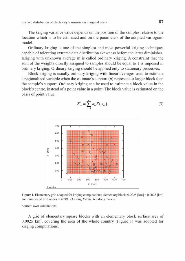
Figure 1. Elementary grid adopted for kriging computations; elementary block: 0.0025 [km] × 0.0025 [km] and number of grid nodes = 4599: 73 along X-axis, 63 along Y-axis
Source: own calculations.
A grid of elementary square blocks with an elementary block surface area of 0.0025 km2, covering the area of the whole country (Figure 1) was adopted for kriging computations.
Ekonometria 1_(39)_Dziechciarz.indb 87 2013-08-23 12:48:46
88 Barbara Namysłowska-Wilczyńska, Artur Wilczyński
3. Results of estimating surface distribution of marginal electricity transmission costs
Averages Z* and estimation standard deviation σk of marginal costs were estimated for 4599 nodes of the elementary grid covering the whole area of the country (Figure 1) (Tables 1–4). The unique neighbourhood (a sample search sub-area) and the moving neighbourhood were taken into account in the kriging computations (Figures 2, 3, 5, 6, 8, 9, 11, 12).
A comparison of the global statistics results for the summer season shows slightly lower Z*min and Z*max values (for the night off-peak period and the morning peak) and slightly higher standard deviations for estimated averages Z* and variation coefficients V (for the summer night off-peak period) when the moving neighbourhood was used (Table 1). In the case of the summer morning peak, lower Z*min, Z*max
values and average *Z were obtained when the moving neighbourhood was used (Table 1). Averages *Z are almost identical for the same time moments of the analysed seasons.
Table 1. Global statistics of estimated averages Z* of marginal costs in nodes of 220 kV and 400 kV networks for the summer season of 2000
Analyzed parameter
Z*min[PLN/MWh]
Z*max[PLN/MWh]
Average *Z [PLN/MWh]
Standard deviation S
[PLN/MWh]
Variation coefficient V
[%]
Skewness
g1
Kurtosis
g2
Summer night off-peak period* 35.17 39.14 37.55 0.92 2.00 –0.23 2.06Summer night off-peak period** 35.16 39.11 37.55 0.94 3.00 –0.22
1.97
Summer morning peak* 49.87 54.87 52.96 1.44 3.00 –0.57 2.12Summer morning peak** 49.68 55.34 52.93 1.44 3.00 –0.50 2.13
* – unique neighbourhood, ** – moving neighbourhood.
Source: own calculations.
Higher minimal Z*min, maximal Z*max values of estimated averages Z*, average *Z and the standard deviation are characteristic of the summer morning peak (Table
1). The very low negative values of skewness coefficient g1 for the distributions of averages Z* indicate that the latter are slightly underestimated (Table 1). The distributions of averages Z* are flattened, which is confirmed by the very low values of kurtosis coefficient g2.
Ekonometria 1_(39)_Dziechciarz.indb 88 2013-08-23 12:48:46

Surface distribution of electricity transmission marginal costs 89
Similar conclusions as for the summer season emerge from an analysis of the kriging computation results for the winter season (Table 2). When the moving neighbourhood is taken into account in the computations, lower values of Z*min, Z*max, of the average *Z and the slightly lower values of the standard deviation and the identical value of variation coefficient V are obtained. Higher values of Z*min, Z*max and of the average of averages *Z and lower values of the standard deviation and of cost variation coefficient V are a characteristic of the winter morning peak, whereas the higher values of the standard deviation and coefficient V were obtained for the winter night off-peak period.
The low positive skewness coefficients g1 of the distributions of averages Z* (except for the winter morning peak) indicate that the latter were slightly overestimated and, in the case of the winter morning peak, quite accurately estimated (Table 2). Similarly as in the case of the summer season, the very low values of kurtosis coefficient g2 indicate that the histograms are flattened.
A comparison of the computed global statistics of estimated cost averages Z* (Tables 1, 2) and the basic statistical parameters of original costs Z (Part I., Tables 1, 2) shows good agreement between the values, regardless of the neighbourhood used. To sum up, the results of the computations carried out using the moving neighbourhood are more accurate (close to the real costs), especially for the winter season.
Table 2. Global statistics of estimated averages Z* of marginal costs in nodes of 220 kV and 400 kV networks for the winter season of 2000
Analyzed parameter
Z*min[PLN/MWh]
Z*max[PLN/MWh]
Average *Z [PLN/MWh]
Standard deviation S
[PLN/MWh]
Variation coefficient V
[%]
Skewness
g1
Kurtosis
g2
Winter night off-peak period* 53.34 64.09 57.14 2.96
5.00 0.53 2.06
Winter night off-peak period** 51.77 62.93 56.99 2.87 5.00 0.37 1.75Winter morning peak* 56.66 64.30 60.42 2.08 3.00 –0.09 1.78 Winter morning peak** 56.18 66.16 60.39 2.16 4.00 4.00 1.90
* – unique neighbourhood, ** – moving neighbourhood.
Source: own calculations.
Two very extensive sub-areas of respectively the highest and lowest averages Z* (38.13÷39.11 PLN/MWh; 35.18÷36.65 PLN/MWh), and a band of intermediate values of Z* (38.13÷36.65 PLN/MWh) are visible on the raster map of the surface distribution of estimated cost averages Z* for the summer night off-peak period (Figures 2, 3). The boundaries of the ranges of averages Z* are very similar for the
Ekonometria 1_(39)_Dziechciarz.indb 89 2013-08-23 12:48:46

90 Barbara Namysłowska-Wilczyńska, Artur Wilczyński
two neighbourhoods used in kriging, becoming less smooth and more irregular in the case of the moving neighbourhood (Figures 2, 3).
When the moving neighbourhood (Figure 3) was used, a sub-area with the highest averages Z* and with the smaller surface area and a different shape than the one obtained in the case of the unique neighbourhood appeared (Figure 2), whereas the sub-area with the lowest averages Z* was more pronounced and had a larger surface area.
Figure 2. Raster map of estimated averages Z* of marginal costs [PLN/MWh] in nodes of 220 kV and 400 kV networks for summer night off-peak period (unique neighbourhood – sample search sub-area)
Source: own calculations.
Figure 3. Raster map of estimated averages Z* of marginal costs [PLN/MWh] in nodes of 220 kV and 400 kV networks for summer night off-peak period (moving neighbourhood – sample search sub-area)
Source: own calculations.
Ekonometria 1_(39)_Dziechciarz.indb 90 2013-08-23 12:48:46

Surface distribution of electricity transmission marginal costs 91
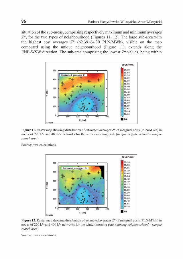
The above ranges of cost averages Z* for the summer night off-peak period, visible on the raster maps (Figures 2, 3), are clearly reflected by the histogram of the distribution of estimated averages Z* (Figure 4) computed using the moving neighbourhood. The classes ranges comprising the maximum averages Z* (38.35÷38.61 [PLN/MWh]) and lower averages Z* (36.74÷37.00 [PLN/MWh]) have very large shares.
Figure 4. Histogram showing distribution of estimated averages Z* of marginal costs [PLN/MWh] nodes of 220 kV and 400 kV networks for summer night off-peak period (moving neighbourhood)
Source: own calculations.
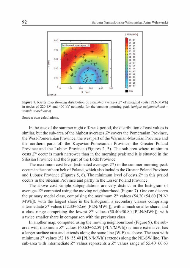
On the raster maps of the distribution of cost averages Z* for the summer morning peak, calculated using the unique neighbourhood (Figure 5), one can discern two very distinct centres, being sub-areas with the highest and lowest averages Z* (53.62÷54.87 PLN/MWh; 49.87÷51.43 PLN/MWh), and a band of intermediate values Z* (51.43÷53.62 PLN/MWh). The boundaries of the ranges of averages Z* do not show similarity for the two neighbourhoods used (Figures 5, 6), as was observed on the map for the night off-peak period (Figures 2, 3).
The raster map computed using the moving neighbourhood shows a slightly smaller, more irregular sub-area with maximum averages Z* (Figure 6). The shape of the sub-area with lowest averages Z* is even more irregular. The calculated ranges of estimated costs averages Z* are: 53.93÷55.34 PLN/MWh (maximum Z* values), 49.68÷51.80 PLN/MWh (minimum Z* values) and 51.80÷53.93 PLN/MWh (intermediate Z* values). The boundaries separating the sub-areas of Z* values are irregular (Figure 6) and not as smooth as the ones on the map computed using the unique neighbourhood (Figure 5).
Ekonometria 1_(39)_Dziechciarz.indb 91 2013-08-23 12:48:46
92 Barbara Namysłowska-Wilczyńska, Artur Wilczyński
Figure 5. Raster map showing distribution of estimated averages Z* of marginal costs [PLN/MWh] in nodes of 220 kV and 400 kV networks for the summer morning peak (unique neighbourhood – sample search area)
Source: own calculations.
In the case of the summer night off-peak period, the distribution of cost values is similar, but the sub-area of the highest averages Z* covers the Pomeranian Province, the West-Pomeranian Province, the west part of the Warmian-Masurian Province and the northern parts of: the Kuyavian-Pomeranian Province, the Greater Poland Province and the Lubusz Province (Figures 2, 3). The sub-area where minimum costs Z* occur is much narrower than in the morning peak and it is situated in the Silesian Province and the S part of the Łódź Province.
The maximum cost level (estimated averages Z*) in the summer morning peak occurs in the northern belt of Poland, which also includes the Greater Poland Province and Lubusz Province (Figures 5, 6). The minimum level of costs Z* in this period occurs in the Silesian Province and partly in the Lesser Poland Province.
The above cost sample subpopulations are very distinct in the histogram of averages Z* computed using the moving neighbourhood (Figure 7). One can discern the primary modal class, comprising the maximum Z* values (54.20÷54.60 [PLN/MWh]), with the largest share in the histogram, a secondary classes comprising intermediate Z* values (52.33÷52.66 [PLN/MWh]), with a much smaller share, and a class range comprising the lowest Z* values (50.40÷50.80 [PLN/MWh]), with a twice smaller share in comparison with the previous class.
In another map, computed using the moving neighbourhood (Figure 9), the sub-area with maximum Z* values (60.63÷62.59 [PLN/MWh]) is more extensive, has a larger surface area and extends along the same line (W-E) as above. The area with minimum Z* values (52.18÷55.40 [PLN/MWh]) extends along the NE-SW line. The sub-area with intermediate Z* values represents a Z* values range of 55.40÷60.63
Ekonometria 1_(39)_Dziechciarz.indb 92 2013-08-23 12:48:46
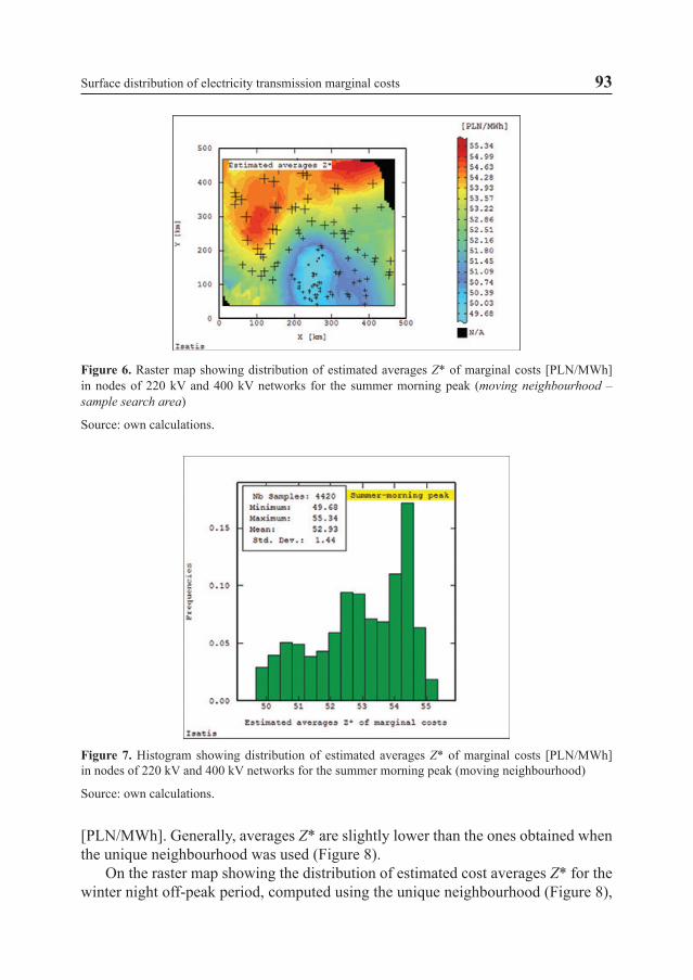
Surface distribution of electricity transmission marginal costs 93
[PLN/MWh]. Generally, averages Z* are slightly lower than the ones obtained when the unique neighbourhood was used (Figure 8).
On the raster map showing the distribution of estimated cost averages Z* for the winter night off-peak period, computed using the unique neighbourhood (Figure 8),
Figure 6. Raster map showing distribution of estimated averages Z* of marginal costs [PLN/MWh] in nodes of 220 kV and 400 kV networks for the summer morning peak (moving neighbourhood – sample search area)
Source: own calculations.
Figure 7. Histogram showing distribution of estimated averages Z* of marginal costs [PLN/MWh] in nodes of 220 kV and 400 kV networks for the summer morning peak (moving neighbourhood)
Source: own calculations.
Ekonometria 1_(39)_Dziechciarz.indb 93 2013-08-23 12:48:46

94 Barbara Namysłowska-Wilczyńska, Artur Wilczyński
one can see two sub-areas: a sub-area with maximum Z* values (61.40÷64.09 [PLN/MWh], located along the W-E line and a sub-area with minimum Z* values (53.34÷56.70 [PLN/MWh]), extending in the ENE-WSW direction (Figure 9). A sub-area containing intermediate Z* values (56.70÷61.40 [PLN/MWh]) is situated between the two above mentioned sub-areas.
Figure 8. Raster map showing distribution of estimated averages Z* of marginal costs [PLN/MWh] in nodes of 220 kV and 400 kV networks for the winter night off-peak period (unique neighbourhood – sample search area)
Source: own calculations.
Figure 9. Raster map showing distribution of estimated averages Z* of marginal costs [PLN/MWh] in nodes of 220 kV and 400 kV networks for the winter night off-peak period (moving neighbourhood – sample search area)
Source: own calculations.
Ekonometria 1_(39)_Dziechciarz.indb 94 2013-08-23 12:48:46

Surface distribution of electricity transmission marginal costs 95
In the histogram showing the distribution of estimated averages Z*, computed using the moving neighbourhood (Figure 10), there is one modal class having the largest share – a range comprising the lower values of Z* (53.88÷54.63 [PLN/MWh]), and other secondary classes containing higher values of Z*, having equal shares.
In the histogram showing the distribution of estimated averages Z*, computed using the moving neighbourhood (Figure 10), there is one modal class having the largest share – a range comprising the lower values of Z* (53.88÷54.63 [PLN/MWh]), and other secondary classes containing higher values of Z*, having equal shares.
Figure 10. Histogram showing of distribution of estimated averages Z* of marginal costs [PLN/MWh] in nodes of 220 kV and 400 kV networks for the winter night off-peak period (moving neighbourhood)
Source: own calculations.
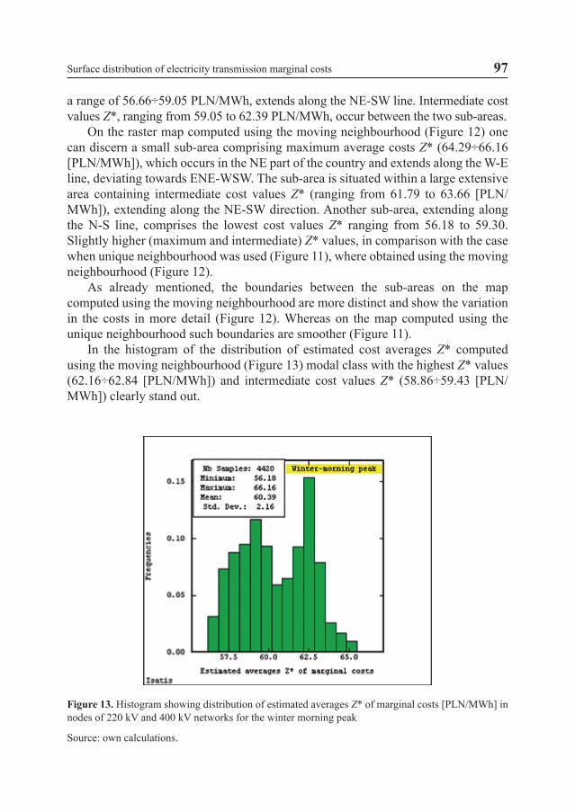
The raster maps of the distribution of estimated cost averages Z*, computed for the winter morning peak, show images differing in the surface area, shape and situation of the sub-areas, comprising respectively maximum and minimum averages Z*, for the two types of neighbourhood (Figures 11, 12). The large sub-area with the highest cost averages Z* (62.39÷64.30 PLN/MWh), visible on the map computed using the unique neighbourhood (Figure 11), extends along the ENE-WSW direction. The sub-area comprising the lowest Z* values, being within a range of 56.66÷59.05 PLN/MWh, extends along the NE-SW line. Intermediate cost values Z*, ranging from 59.05 to 62.39 PLN/MWh, occur between the two sub-areas.
The raster maps of the distribution of estimated cost averages Z*, computed for the winter morning peak, show images differing in the surface area, shape and
Ekonometria 1_(39)_Dziechciarz.indb 95 2013-08-23 12:48:46
96 Barbara Namysłowska-Wilczyńska, Artur Wilczyński
situation of the sub-areas, comprising respectively maximum and minimum averages Z*, for the two types of neighbourhood (Figures 11, 12). The large sub-area with the highest cost averages Z* (62.39÷64.30 PLN/MWh), visible on the map computed using the unique neighbourhood (Figure 11), extends along the ENE-WSW direction. The sub-area comprising the lowest Z* values, being within
Figure 11. Raster map showing distribution of estimated averages Z* of marginal costs [PLN/MWh] in nodes of 220 kV and 400 kV networks for the winter morning peak (unique neighbourhood – sample search area)
Source: own calculations.
Figure 12. Raster map showing distribution of estimated averages Z* of marginal costs [PLN/MWh] in nodes of 220 kV and 400 kV networks for the winter morning peak (moving neighbourhood – sample search area)
Source: own calculations.
Ekonometria 1_(39)_Dziechciarz.indb 96 2013-08-23 12:48:47
Surface distribution of electricity transmission marginal costs 97
a range of 56.66÷59.05 PLN/MWh, extends along the NE-SW line. Intermediate cost values Z*, ranging from 59.05 to 62.39 PLN/MWh, occur between the two sub-areas.
On the raster map computed using the moving neighbourhood (Figure 12) one can discern a small sub-area comprising maximum average costs Z* (64.29÷66.16 [PLN/MWh]), which occurs in the NE part of the country and extends along the W-E line, deviating towards ENE-WSW. The sub-area is situated within a large extensive area containing intermediate cost values Z* (ranging from 61.79 to 63.66 [PLN/MWh]), extending along the NE-SW direction. Another sub-area, extending along the N-S line, comprises the lowest cost values Z* ranging from 56.18 to 59.30. Slightly higher (maximum and intermediate) Z* values, in comparison with the case when unique neighbourhood was used (Figure 11), where obtained using the moving neighbourhood (Figure 12).
As already mentioned, the boundaries between the sub-areas on the map computed using the moving neighbourhood are more distinct and show the variation in the costs in more detail (Figure 12). Whereas on the map computed using the unique neighbourhood such boundaries are smoother (Figure 11).
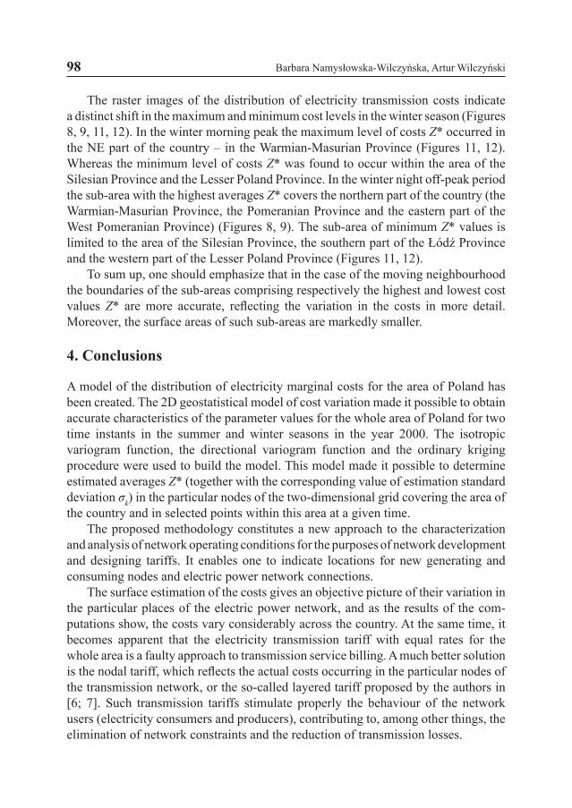
In the histogram of the distribution of estimated cost averages Z* computed using the moving neighbourhood (Figure 13) modal class with the highest Z* values (62.16÷62.84 [PLN/MWh]) and intermediate cost values Z* (58.86÷59.43 [PLN/MWh]) clearly stand out.
Figure 13. Histogram showing distribution of estimated averages Z* of marginal costs [PLN/MWh] in nodes of 220 kV and 400 kV networks for the winter morning peak
Source: own calculations.
Ekonometria 1_(39)_Dziechciarz.indb 97 2013-08-23 12:48:47
98 Barbara Namysłowska-Wilczyńska, Artur Wilczyński
The raster images of the distribution of electricity transmission costs indicate a distinct shift in the maximum and minimum cost levels in the winter season (Figures 8, 9, 11, 12). In the winter morning peak the maximum level of costs Z* occurred in the NE part of the country – in the Warmian-Masurian Province (Figures 11, 12). Whereas the minimum level of costs Z* was found to occur within the area of the Silesian Province and the Lesser Poland Province. In the winter night off-peak period the sub-area with the highest averages Z* covers the northern part of the country (the Warmian-Masurian Province, the Pomeranian Province and the eastern part of the West Pomeranian Province) (Figures 8, 9). The sub-area of minimum Z* values is limited to the area of the Silesian Province, the southern part of the Łódź Province and the western part of the Lesser Poland Province (Figures 11, 12).
To sum up, one should emphasize that in the case of the moving neighbourhood the boundaries of the sub-areas comprising respectively the highest and lowest cost values Z* are more accurate, reflecting the variation in the costs in more detail. Moreover, the surface areas of such sub-areas are markedly smaller.
4. Conclusions
A model of the distribution of electricity marginal costs for the area of Poland has been created. The 2D geostatistical model of cost variation made it possible to obtain accurate characteristics of the parameter values for the whole area of Poland for two time instants in the summer and winter seasons in the year 2000. The isotropic variogram function, the directional variogram function and the ordinary kriging procedure were used to build the model. This model made it possible to determine estimated averages Z* (together with the corresponding value of estimation standard deviation σk) in the particular nodes of the two-dimensional grid covering the area of the country and in selected points within this area at a given time.
The proposed methodology constitutes a new approach to the characterization and analysis of network operating conditions for the purposes of network development and designing tariffs. It enables one to indicate locations for new generating and consuming nodes and electric power network connections.
The surface estimation of the costs gives an objective picture of their variation in the particular places of the electric power network, and as the results of the com-putations show, the costs vary considerably across the country. At the same time, it becomes apparent that the electricity transmission tariff with equal rates for the whole area is a faulty approach to transmission service billing. A much better solution is the nodal tariff, which reflects the actual costs occurring in the particular nodes of the transmission network, or the so-called layered tariff proposed by the authors in [6; 7]. Such transmission tariffs stimulate properly the behaviour of the network users (electricity consumers and producers), contributing to, among other things, the elimination of network constraints and the reduction of transmission losses.
Ekonometria 1_(39)_Dziechciarz.indb 98 2013-08-23 12:48:47
Surface distribution of electricity transmission marginal costs 99
In the dynamically changing electricity market conditions, the use of the surface methods of estimating marginal costs is one of the factors minimizing the system costs of electricity supply. The proposed methods can be useful for the planning of investments in the electric power network infrastructure.
Literature
[1] Armstrong M., Basic Linear Geostatistics, Springer, Berlin 1998.[2] Isaaks E.H., Srivastava R.M., An Introduction to Applied Geostatistics, Oxford University Press,
New York, Oxford 1989.[3] Namysłowska-Wilczyńska B., Geostatystyka – teoria i zastosowania, Oficyna Wydawnicza Poli-
techniki Wrocławskiej, Wrocław 2006.[4] Namysłowska-Wilczyńska B., Tymorek A., Wilczyński A., Modelowanie zmian kosztów krańco-
wych przesyłu energii elektrycznej z wykorzystaniem metod statystyki przestrzennej, XI Międzyna-rodowa Konferencja Naukowa nt. Aktualne problemy w elektroenergetyce APE’03, Politechnika Gdańska, Jurata 11–13.06.2003, pp. 217–224.
[5] Namysłowska-Wilczyńska B., Wilczyński A., 3D electric power demand as tool for planning electrical power firm’s activity by means of geostatistical methods. Econometrics. Forecasting No 28, Research Papers of Wrocław University of Economics No 91, Wrocław 2010, pp. 95–112.
[6] Tymorek A., Wilczyński A., Transmission Tariff Structure – Assessment and Modification Sugges-tions, Proceedings of the International Symposium “Modern Electric Power Systems” MEPS’02, Wrocław University of Technology, Wrocław, 11–13 September, 2002, pp. 31–35.
[7] Tymorek A., Namysłowska-Wilczyńska B., Wilczyński A., Koncepcja warstwowej taryfy przesy-łowej, Rynek Energii nr 2 (93), 2011, s. 106–111.
MODEL GEOSTATYSTYCZNY (2D) POWIERZCHNIOWEGO ROZKŁADU KOSZTÓW MARGINALNYCH PRZESYŁU ENERGII ELEKTRYCZNEJ
Streszczenie: W artykule przedstawiono sposób budowy powierzchniowego modelu kosztów krańcowych przesyłu energii elektrycznej siecią 220 kV i 400 kV. Wykorzystując rezultaty analizy strukturalnej zmienności kosztów, zastosowano estymacyjną technikę krigingu zwy-czajnego (blokowego). Opracowany model opisujący zmienność obszarową i czasową kosz-tów marginalnych ma duże walory aplikacyjne w sektorze elektroenergetycznym, szczególnie w sytuacji rozwijania mechanizmów rynkowych w obrocie energią elektryczną. Model ten umożliwił zaobserwowanie istniejących tendencji zróżnicowania kosztów – czasowej i kie-runkowej, co jest przydatne w tworzeniu taryf przesyłowych energii elektrycznej, właściwie stymulujących postępowanie użytkowników sieci elektroenergetycznej – dostawców oraz konsumentów energii elektrycznej. Taki sposób stymulowania uwzględnia wówczas specyfikę i warunki pracy sieci elektroenergetycznej, w tym straty sieciowe, spowodowane przesyłem energii, ograniczenia przesyłowe i szeroko rozumiane bezpieczeństwo pracy systemu elektro-energetycznego. Model obszarowej zmienności kosztów marginalnych przesyłu energii elek-trycznej jest również przydatny w planowaniu rozwoju systemu elektroenergetycznego.
Słowa kluczowe: koszty krańcowe przesyłu, zmienność kosztów, energia elektryczna, esty-macja powierzchniowego rozkładu kosztów, kriging zwyczajny (blokowy).
Ekonometria 1_(39)_Dziechciarz.indb 99 2013-08-23 12:48:47